Most traders have seen the “bell curve” at some point, but very few actually use it when they think about risk and returns.
If you really understand the normal distribution, you’re already thinking more like a risk manager than a gambler.
1. What is the normal distribution?
The normal distribution is a probability distribution that describes how values tend to cluster around an average.
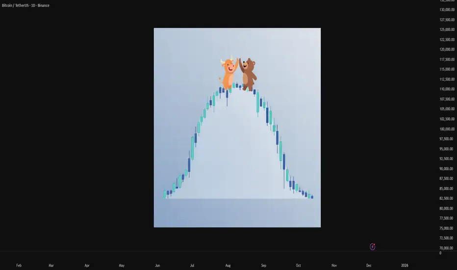
If you plotted a huge number of outcomes (for example, daily returns or P&L per trade), the shape you’d get would often look like a symmetric bell:
- Most observations are close to the center.
- As you move away from the center in either direction, outcomes become less frequent.
- Extreme gains and losses are possible, but they’re relatively rare.
Mathematically, a normal distribution is usually written as N(μ, σ):
μ (mu) is the mean – the average outcome.
σ (sigma) is the standard deviation – a measure of how widely the outcomes are spread around that mean.
In trading terms:
If your returns roughly follow a normal distribution, you should expect many small wins and losses clustered near zero, and only occasional large moves in either direction.
2. Mean (μ): the “drift” of your system
The mean is the point at the center of the distribution. On a chart of returns, this is where the bell is highest.
If μ > 0, the bell is shifted slightly to the right → your system is profitable on average.
If μ < 0, it’s shifted to the left → your system slowly loses money over time.
For a trading strategy, μ is basically your edge. It doesn’t need to be huge. Even a small positive mean return, if it’s consistent and combined with disciplined risk management, can compound strongly over the long run.
3. Standard deviation (σ): volatility in one number
The standard deviation controls how wide or narrow the bell curve is.
- A small σ gives a tall, narrow bell → outcomes are tightly clustered around the mean.
- A large σ gives a short, wide bell → outcomes are more spread out, with bigger swings away from the mean.
Think of σ as a statistical way to describe volatility:
- For an asset: how much its price typically moves relative to its average change.
- For your strategy: how much your returns or daily P&L fluctuate.
Two systems can have the same mean return but very different σ:
- System A: μ = 0.2%, σ = 0.5% → relatively smooth ride.
- System B: μ = 0.2%, σ = 2% → same edge, but a wild equity curve and deeper drawdowns.
Same average, totally different emotional and risk profile.

4. The 68–95–99.7 rule
One of the most useful features of the normal distribution is how predictable it is. Roughly:
- About 68.2% of observations lie within ±1σ of the mean.
- About 95.4% lie within ±2σ.
- About 99.7% lie within ±3σ.
So if daily returns of an asset were approximately normal with:
- Mean μ = 0.1%
- Standard deviation σ = 1%
Then under that model you’d expect:
- Roughly 68% of days between –0.9% and +1.1%
- Roughly 95% of days between –1.9% and +2.1%
- Only about 0.3% of days beyond ±3%
Anything far outside that ±3σ range is, in theory, a very rare event. In practice, that’s often the kind of day everyone remembers.

5. Why this matters for traders
Even with all its limitations, the normal distribution is a powerful framework for thinking about risk:
Position sizing
If you know (or estimate) the standard deviation of your returns, you can form an idea of what “normal” daily or weekly swings look like, and size positions so those swings are survivable.
Stop-loss logic
Stops that sit right in the middle of the usual noise (within about ±1σ) will get hit constantly.
Stops closer to the ±2σ–3σ region are more aligned with “something unusual is happening, I want to be out.”
Expectation management
Most days and most trades will fall inside the “boring” part of the bell curve.
Understanding that prevents you from overtrading while you wait for the edges of the distribution – the bigger opportunities.
6. The catch: markets are not perfectly normal
Real markets often break the textbook assumptions:
- Returns tend to have fat tails → extreme moves happen more often than a normal distribution would predict.
- Distributions are often skewed → one side (usually the downside) has more frequent or more severe extreme events.
That means:
- A move that looks like a “5σ event” under a normal model might actually be something that happens every few years.
- Risk models based strictly on normal assumptions usually underestimate crash risk.
- Strategies like option selling can look very safe when you only think in terms of a normal distribution, but they are very sensitive to those fat tails.
So the normal distribution should be treated as a baseline model, not as reality itself.
7. Quick recap
The normal distribution is the classic bell curve that describes how values cluster around an average.
It’s parameterized by μ (mean) and σ (standard deviation).
Roughly 68% / 95% / 99.7% of observations lie within 1σ / 2σ / 3σ of the mean in a perfectly normal world.
Markets only approximate this; they usually show fat tails and skew, so extreme events are more common than the simple model suggests.
Even with those limitations, it’s a very useful tool for thinking about returns, drawdowns, and the range of outcomes you should be prepared for.
If you really understand the normal distribution, you’re already thinking more like a risk manager than a gambler.
1. What is the normal distribution?
The normal distribution is a probability distribution that describes how values tend to cluster around an average.
If you plotted a huge number of outcomes (for example, daily returns or P&L per trade), the shape you’d get would often look like a symmetric bell:
- Most observations are close to the center.
- As you move away from the center in either direction, outcomes become less frequent.
- Extreme gains and losses are possible, but they’re relatively rare.
Mathematically, a normal distribution is usually written as N(μ, σ):
μ (mu) is the mean – the average outcome.
σ (sigma) is the standard deviation – a measure of how widely the outcomes are spread around that mean.
In trading terms:
If your returns roughly follow a normal distribution, you should expect many small wins and losses clustered near zero, and only occasional large moves in either direction.
2. Mean (μ): the “drift” of your system
The mean is the point at the center of the distribution. On a chart of returns, this is where the bell is highest.
If μ > 0, the bell is shifted slightly to the right → your system is profitable on average.
If μ < 0, it’s shifted to the left → your system slowly loses money over time.
For a trading strategy, μ is basically your edge. It doesn’t need to be huge. Even a small positive mean return, if it’s consistent and combined with disciplined risk management, can compound strongly over the long run.
3. Standard deviation (σ): volatility in one number
The standard deviation controls how wide or narrow the bell curve is.
- A small σ gives a tall, narrow bell → outcomes are tightly clustered around the mean.
- A large σ gives a short, wide bell → outcomes are more spread out, with bigger swings away from the mean.
Think of σ as a statistical way to describe volatility:
- For an asset: how much its price typically moves relative to its average change.
- For your strategy: how much your returns or daily P&L fluctuate.
Two systems can have the same mean return but very different σ:
- System A: μ = 0.2%, σ = 0.5% → relatively smooth ride.
- System B: μ = 0.2%, σ = 2% → same edge, but a wild equity curve and deeper drawdowns.
Same average, totally different emotional and risk profile.
4. The 68–95–99.7 rule
One of the most useful features of the normal distribution is how predictable it is. Roughly:
- About 68.2% of observations lie within ±1σ of the mean.
- About 95.4% lie within ±2σ.
- About 99.7% lie within ±3σ.
So if daily returns of an asset were approximately normal with:
- Mean μ = 0.1%
- Standard deviation σ = 1%
Then under that model you’d expect:
- Roughly 68% of days between –0.9% and +1.1%
- Roughly 95% of days between –1.9% and +2.1%
- Only about 0.3% of days beyond ±3%
Anything far outside that ±3σ range is, in theory, a very rare event. In practice, that’s often the kind of day everyone remembers.
5. Why this matters for traders
Even with all its limitations, the normal distribution is a powerful framework for thinking about risk:
Position sizing
If you know (or estimate) the standard deviation of your returns, you can form an idea of what “normal” daily or weekly swings look like, and size positions so those swings are survivable.
Stop-loss logic
Stops that sit right in the middle of the usual noise (within about ±1σ) will get hit constantly.
Stops closer to the ±2σ–3σ region are more aligned with “something unusual is happening, I want to be out.”
Expectation management
Most days and most trades will fall inside the “boring” part of the bell curve.
Understanding that prevents you from overtrading while you wait for the edges of the distribution – the bigger opportunities.
6. The catch: markets are not perfectly normal
Real markets often break the textbook assumptions:
- Returns tend to have fat tails → extreme moves happen more often than a normal distribution would predict.
- Distributions are often skewed → one side (usually the downside) has more frequent or more severe extreme events.
That means:
- A move that looks like a “5σ event” under a normal model might actually be something that happens every few years.
- Risk models based strictly on normal assumptions usually underestimate crash risk.
- Strategies like option selling can look very safe when you only think in terms of a normal distribution, but they are very sensitive to those fat tails.
So the normal distribution should be treated as a baseline model, not as reality itself.
7. Quick recap
The normal distribution is the classic bell curve that describes how values cluster around an average.
It’s parameterized by μ (mean) and σ (standard deviation).
Roughly 68% / 95% / 99.7% of observations lie within 1σ / 2σ / 3σ of the mean in a perfectly normal world.
Markets only approximate this; they usually show fat tails and skew, so extreme events are more common than the simple model suggests.
Even with those limitations, it’s a very useful tool for thinking about returns, drawdowns, and the range of outcomes you should be prepared for.
Disclaimer
The information and publications are not meant to be, and do not constitute, financial, investment, trading, or other types of advice or recommendations supplied or endorsed by TradingView. Read more in the Terms of Use.
Disclaimer
The information and publications are not meant to be, and do not constitute, financial, investment, trading, or other types of advice or recommendations supplied or endorsed by TradingView. Read more in the Terms of Use.