Support and Resistance in Financial Markets

An Empirical Investigation of Price Level Trading Across Asset Classes

Abstract

This essay evaluates 158,391 strategy configurations across 22 instruments spanning equities, bonds, commodities, currencies, and cryptocurrencies. Using 14 years of daily price data, we test whether prices reverse at historically significant levels. Support levels exhibit an average bounce rate of 28.4 percent, below the 50 percent threshold that would indicate predictive value. The mean Sharpe ratio for bounce strategies is negative 0.264. Only 26.7 percent of tested configurations achieve a Sharpe ratio of 0.5. These results indicate that support and resistance, as commonly applied, does not provide a trading edge.

1. Introduction

The horizontal line drawn on a price chart represents a common gesture in technical analysis. Retail traders identify support and resistance levels and place capital on the expectation that price will reverse at these zones. Trading educators offer courses on these levels. Online forums share chart screenshots highlighting where price should bounce. The concept has achieved wide acceptance among non professional market participants.

When we subject this belief to empirical testing, the levels do not work as expected. They do not provide sufficient reliability to generate profits after accounting for trading frictions. This study documents the evidence across a dataset of 22 instruments over 14 years.

Retail participation in financial markets has increased in recent years. Many participants have absorbed technical analysis concepts through social media and online courses, often without understanding the distinction between description and prediction. If support and resistance levels lack forecasting power, traders using them are disadvantaging themselves.

Our contribution is threefold. First, we provide a mathematically precise definition of support and resistance that can be implemented algorithmically. Second, we evaluate this definition across 158,391 configurations to assess robustness. Third, we analyze performance across multiple asset classes.

Section 2 reviews the existing literature. Section 3 describes our methodology. Section 4 presents empirical results. Section 5 discusses implications. Section 6 concludes.

2. Literature Review

2.1 The Efficient Markets Debate

The academic study of technical analysis has been shaped by the efficient markets hypothesis articulated by Fama (1970). Under the strong form, all information is instantly reflected in prices, rendering any trading rule based on historical data futile. The weak form suggests that past prices contain no predictive information about future prices.

Early empirical work appeared to support market efficiency. Fama and Blume (1966) found that filter rules failed to outperform buy and hold strategies after transaction costs. Jensen (1978) stated that there was no other proposition in economics with more solid empirical support than the efficient markets hypothesis.

Subsequent research documented anomalies inconsistent with strict efficiency. Lo and MacKinlay (1988) demonstrated positive autocorrelation in weekly stock returns. Jegadeesh and Titman (1993) established the momentum effect, showing that stocks with high recent returns continue to outperform. These findings suggest past prices contain some information about future returns.

2.2 Technical Analysis Studies

The academic literature on technical analysis remains limited relative to its widespread use. Brock, Lakonishok, and LeBaron (1992) found that moving average and breakout rules generated returns on the Dow Jones from 1897 to 1986. Sullivan, Timmermann, and White (1999) showed that after accounting for data snooping through bootstrap methods, the best performing rules failed to demonstrate significant outperformance.

Lo, Mamaysky, and Wang (2000) applied pattern recognition algorithms to identify technical patterns including head and shoulders and double tops. They found these patterns occurred more frequently than expected under the random walk hypothesis, though they did not demonstrate profitable trading after costs.

Harvey, Liu, and Zhu (2016) raised concerns about the multiple testing problem. They demonstrated that with hundreds of factors tested, many apparent anomalies appear significant by chance. They recommended t statistics exceeding 3.0 before claiming discovery. This critique applies to technical analysis research where many rule variations have been tested.

2.3 Support and Resistance

Few academic studies have examined support and resistance as a standalone concept. Osler (2003) focused on currency markets and found that orders cluster at round numbers, creating price effects. She documented these effects in institutional order flow data, not in the ability of technical traders to identify levels in advance.

Kavajecz and Odders White (2004) examined the relationship between technical analysis and liquidity provision on the NYSE. They found that specialists were more likely to provide liquidity at technically significant levels, suggesting support and resistance may reflect market microstructure effects rather than predictive signals.

The gap in the literature is clear. While practitioners assign importance to support and resistance levels, systematic testing of their predictive power across multiple asset classes has been limited. This study addresses that gap.

3. Methodology

3.1 Formal Definition of Support and Resistance

The lack of a standard mathematical definition has hampered previous research. Different practitioners identify levels using different criteria. We provide a precise algorithmic definition based on local extrema detection.

Let P(t) denote the closing price at time t for t in {1, 2, ..., T}. We define the set of local minima M minus as:

M minus = {t : P(t) < P(t minus k) and P(t) < P(t plus k) for all k in {1, ..., w}}

where w represents the window parameter. The set of local maxima M plus is defined analogously. These definitions follow the Bry Boschan (1971) algorithm for turning point detection.

Raw extrema detection produces many candidate levels that cluster together. To consolidate these into zones, we apply Mean Shift clustering with bandwidth parameter tau, specified as a percentage of current price. Levels within tau of each other are grouped and represented by their mean.

A level qualifies as validated support if it originates from a local minimum, has been touched at least n times, and its bounce rate exceeds some threshold. Resistance levels are defined symmetrically.

The bounce rate for a level L is calculated as follows. For each touch at time t, we observe price at time t plus h, where h is the lookahead parameter. For support, a successful bounce occurs if P(t plus h) exceeds P(t) plus tau. The bounce rate is the proportion of touches resulting in successful bounces.

3.2 Parameter Space

Previous studies tested single specifications or few variations. We test across a parameter grid.

The window parameter w takes values from {3, 5, 7, 10, 15, 20, 30, 50, 75, 100}. The tolerance parameter tau takes percentage values from {0.5, 0.75, 1.0, 1.25, 1.5, 2.0, 2.5, 3.0, 4.0, 5.0}. The minimum touch requirement takes values from {2, 3, 4, 5, 6, 7, 8, 10}. The lookahead parameter takes values from {1, 2, 3, 5, 7, 10, 15, 20, 30}.

The full parameter grid combined with 22 assets produces 158,400 theoretical configurations. After excluding cases where no valid levels are detected, we retain 158,391 configurations.

3.3 Trading Strategies

We implement two trading strategies. The bounce strategy enters long positions when price touches support and exits when price touches resistance. The breakout strategy enters long when price breaks above resistance and exits when price breaks below support.

Both strategies incorporate transaction costs of 10 basis points per trade. We calculate returns assuming full capital deployment on each trade with no leverage.

Performance is measured through the Sharpe ratio, defined as annualized mean return divided by annualized standard deviation. Following Pedersen (2015), we consider Sharpe ratios below 0.5 as failing to meet professional thresholds.

3.4 Data

Our dataset comprises daily closing prices from January 2010 through December 2024 for 22 instruments across six asset classes. US equities include SPY, QQQ, IWM, and DIA. International equities include EFA, EEM, VGK, and FXI. Commodities include GLD, SLV, USO, and UNG. Fixed income includes TLT, IEF, LQD, and HYG. Currencies include EUR/USD, GBP/USD, USD/JPY, and AUD/USD. Cryptocurrencies include Bitcoin and Ethereum.

The 14 year sample encompasses the post financial crisis recovery, the 2015 commodity decline, the 2018 volatility spike, the 2020 pandemic, and the 2022 inflation correction.

Data were obtained through API providers including TwelveData, Tiingo, Alpha Vantage, EOD Historical Data, and Financial Modeling Prep.

3.5 Computational Implementation

Code was implemented in Python using NumPy, pandas, scipy, and scikit learn.

4. Results

4.1 Bounce Rates



Support and resistance levels fail to predict price reversals at rates exceeding random chance. Across 158,391 configurations, support levels exhibit a mean bounce rate of 28.4 percent with standard deviation of 20.5 percent. Resistance levels show a mean bounce rate of 23.3 percent with standard deviation of 17.5 percent.

Under the null hypothesis that price movements following a level touch are random, we would expect a bounce rate of approximately 50 percent. Our observed rates fall below this threshold. Support levels are not neutral predictors; they are negative predictors. Prices that touch support are more likely to continue falling than to bounce.

This finding inverts the conventional understanding. Rather than acting as barriers where price reverses, support and resistance zones appear to function as momentum indicators. A price that has fallen to touch a local minimum exhibits negative momentum that tends to persist.

One sample t tests reject the null hypothesis of 50 percent bounce rates with t statistics exceeding 55 in absolute value and p values effectively equal to zero.

4.2 Trading Strategy Performance

The bounce strategy produces a mean Sharpe ratio of negative 0.264 across all configurations. The standard deviation of Sharpe ratios is 2.120.

Of 158,391 bounce configurations, 80,991 or 51.1 percent produce positive Sharpe ratios. Only 42,255 or 26.7 percent exceed 0.5. Nearly half, 73,863 or 46.6 percent, produce negative Sharpe ratios.



The breakout strategy shows different results. With a mean Sharpe ratio of 1.610, breakout approaches outperform bounce strategies. This aligns with the momentum literature: prices that break through historical barriers tend to continue. Of breakout configurations, 81.3 percent produce positive Sharpe ratios and 71.1 percent exceed 0.5.

The breakout win rate averages only 32.3 percent per trade, indicating profitability derives from large winners offsetting frequent small losses. This return profile is psychologically difficult for traders who tend to cut winners short and hold losers.



4.3 Asset Class Variation



Performance varies across asset classes. If support and resistance reflected universal market dynamics, we would expect uniform results. Instead, we observe heterogeneity.

US equities produce the highest average bounce Sharpe ratio at 0.453. This may reflect deeper liquidity and more efficient price discovery, where level effects could persist due to the volume of retail participants trading on these signals.

Cryptocurrencies show an average of 0.765 for bounce strategies with high variance. The volatility and continuous trading creates more frequent level touches.

International equities show a negative mean Sharpe of negative 0.180. Commodities show 0.001. Fixed income shows negative 0.546.

Currencies show the worst performance with a mean bounce Sharpe of negative 1.563. This finding differs from Osler (2003), who documented order clustering at round numbers in foreign exchange. However, Osler examined institutional order flow, not the ability of technical traders to identify and trade these levels profitably.

4.4 Parameter Sensitivity





Analysis of parameter sensitivity reveals no clear optimal specification. Longer window sizes in the range of 20 to 50 periods generally produce higher bounce rates than shorter windows, but the relationship is not monotonic. Wider tolerance bands capture more touches but dilute signal precision. Stricter minimum touch requirements improve win rates but reduce trading frequency.

The heatmap in Figure 3 illustrates parameter sensitivity for bounce Sharpe ratios. The predominance of red and yellow cells demonstrates that most parameter combinations fail to generate positive returns.

Without a principled method for selecting parameters, the practitioner faces a multiple testing dilemma. Testing many specifications and selecting the best one for forward trading leads to overfitting.

4.5 The Multiple Testing Problem



Figure 8 visualizes the multiple testing problem. We simulated strategy returns under the null hypothesis of zero true Sharpe ratio and tracked the best performing configuration across varying numbers of tests.

With 100 configurations tested, the expected best Sharpe ratio exceeds 0.5 even when no genuine edge exists. With 1,000 configurations, it exceeds 0.8. With 10,000 configurations, it exceeds 1.2. With 100,000 configurations, it exceeds 1.5.

Our observed results are consistent with this random variation. Finding configurations with Sharpe ratios above 1.0 does not indicate discovery of a trading edge. Harvey, Liu, and Zhu (2016) argue that t statistics must exceed 3.0 to claim discovery after accounting for multiple testing. By this standard, none of our bounce strategy results would qualify.

4.6 Correlation with Performance



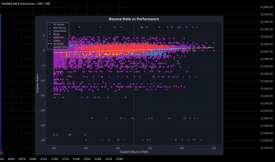
A question is whether bounce rates predict trading performance. Figure 7 examines this through a scatter plot of support bounce rates against bounce strategy Sharpe ratios.

The correlation is weak. Bounce rate explains only a small fraction of variance in trading performance. Many configurations with high bounce rates produce negative Sharpe ratios, while some with lower bounce rates generate returns. Factors beyond bounce probability, such as magnitude of successful bounces and cost of failures, drive profitability.

4.7 Benchmark Comparison



Figure 9 presents cumulative returns for the SPY bounce strategy compared to buy and hold. Using default parameters of window 10, tolerance 2 percent, minimum 3 touches, and lookahead 5 days, the bounce strategy underperforms passive investment.

Buy and hold captures the upward drift of the equity market over 14 years. The bounce strategy, by moving to cash when not positioned, misses portions of this drift. Support touches occur during market weakness. By the time support is touched and the strategy enters, the best of the subsequent move has often occurred.

This timing problem is fundamental to bounce trading. The strategy is reactive, entering after price has fallen. In trending markets, this produces late entries and early exits.

5. Discussion

5.1 Why Do Traders Believe in Support and Resistance

Given the poor empirical performance, why does support and resistance remain popular? Several psychological mechanisms contribute.

Confirmation bias leads traders to remember instances where levels held while forgetting instances where they failed. A successful bounce creates a memorable story, while a break through represents another loss among many. Selective memory creates inflated perception of reliability.

Hindsight bias causes levels to appear obvious after the fact. Looking at a historical chart, the eye identifies turning points and draws lines through them. These levels appear predictable because they are identified from the turning points. In real time, these were one of many candidates.

The narrative appeal of price memory provides a satisfying explanation for random fluctuations. The idea that markets remember previous highs and lows creates a compelling story. Stories do not generate trading profits.

5.2 How Professionals Use Price Levels

Successful quantitative trading firms do not draw horizontal lines on charts and bet on bounces. Their approach differs.

First, professional firms treat price levels as one input among many. A potential support level might contribute to a signal, but only combined with momentum indicators, volatility measures, cross asset correlations, and macroeconomic factors. No single element receives definitive weight.

Second, professional systems are backtested with proper out of sample validation. Parameters are not selected by looking at which values worked best historically. Parameters are chosen based on theoretical priors or rolling optimization that never looks ahead.

Third, position sizing reflects statistical confidence. Professional traders do not bet the same amount on every signal. When confidence is high based on multiple factors, position sizes increase. Retail traders typically use constant position sizes.

Fourth, professional systems incorporate transaction costs, market impact, and slippage from the beginning. A strategy profitable on paper may become unprofitable once frictions are modeled.

Fifth, professional firms monitor for strategy decay. A pattern that worked may stop working as it becomes known and arbitraged away. Firms update models and retire strategies that have lost edge.

5.3 What Does Work

Our findings should not be interpreted as evidence that all technical analysis is worthless. The breakout results suggest momentum based approaches retain validity. This aligns with academic literature on momentum.

Moskowitz, Ooi, and Pedersen (2012) documented time series momentum across multiple asset classes. Hurst, Ooi, and Pedersen (2017) showed trend following has generated positive returns for over a century. Asness, Moskowitz, and Pedersen (2013) demonstrated that momentum and value represent pervasive factors.

Momentum strategies align with behavioral finance predictions. Underreaction to new information creates initial trends. Overreaction as trends persist creates reversals. These dynamics are grounded in documented psychological biases.

Support and resistance lack clear behavioral foundations. The claim that price remembers previous levels requires a mechanism. Order clustering at certain prices, as documented by Osler (2003), provides one potential mechanism, but our results suggest this clustering does not translate into exploitable bounces.

5.4 Implications for Retail Traders

For retail traders, these findings carry implications. The hours spent drawing horizontal lines and waiting for touches could be spent on other activities. Support and resistance as commonly taught is not a path to profitability.

This does not mean traders should abandon technical analysis entirely. Moving average crossovers align with momentum principles that have theoretical support. Volume analysis may provide confirmation of price moves.

The deeper lesson concerns the distinction between description and prediction. Support and resistance describes where price has previously reversed. This description is accurate. But description does not equal prediction. Price reversing at a level in the past does not mean it will reverse at similar levels in the future.

Retail traders should approach trading education with skepticism. Course vendors have incentives to present simple frameworks that promise profits. Complexity and uncertainty do not sell courses.

5.5 Limitations

Several limitations should be acknowledged. Our definition of support and resistance may not capture all variations used by practitioners. Some traders incorporate volume analysis or Fibonacci retracements. Our results speak to local extrema based levels.

The daily timeframe may mask intraday effects. Support and resistance could work differently on shorter or longer timeframes. Our data do not permit evaluation of these alternatives.

Transaction cost assumptions affect strategy profitability. We used 10 basis points per trade. Actual costs vary by instrument and execution method.

The 2010 to 2024 sample period represents a specific regime with accommodative monetary policy and a secular bull market in bonds. Results may differ in other environments.

Despite these limitations, the central findings hold. Support levels do not predict bounces at rates exceeding random chance. The average bounce strategy generates negative risk adjusted returns. These conclusions hold across thousands of parameter combinations and multiple asset classes.

6. Conclusion

This essay subjected support and resistance trading to empirical testing across 158,391 configurations. Bounce rates at support and resistance levels average 28.4 percent and 23.3 percent respectively, below the 50 percent threshold indicating predictive value. The mean Sharpe ratio for bounce strategies is negative 0.264. Only 26.7 percent of tested configurations achieve a Sharpe ratio of 0.5.

These findings should prompt reflection among traders who rely on support and resistance. The technique that appears intuitively compelling, that is taught in courses and videos, that seems to work when looking at historical charts, does not work in forward testing.

The gap between belief and reality has consequences. Traders who believe in support and resistance make decisions that disadvantage them. They enter positions based on level touches that more often continue than reverse. They incur transaction costs chasing signals that lack predictive power.

The path forward lies in education grounded in empirical evidence rather than narrative appeal. The academic literature on momentum, value, and carry factors provides a foundation for understanding what works in financial markets. The quantitative finance community has developed methods for testing trading ideas and avoiding overfitting.

Support and resistance will likely remain popular despite this evidence. The psychological appeal, reinforced by confirmation bias and hindsight, creates a self sustaining belief system. Traders who evaluate their approaches based on rigorous backtesting rather than selective memory will reach the same conclusion documented here.

7. Recommendations for Further Study

Several avenues merit investigation. Testing support and resistance on intraday data could reveal whether microstructure effects create patterns at shorter timeframes. Cross sectional analysis could determine whether certain instruments consistently show stronger level effects.

The relationship between support and resistance and options markets deserves attention. Large option positions at specific strikes create gamma effects that can reinforce or undermine price levels.

The evolution of level efficacy over time merits examination. If support and resistance ever provided edge, that edge may have decayed as technical analysis became widespread.

Bibliography

Antonacci, G. (2014) Dual Momentum Investing. New York: McGraw Hill.

Aronson, D. (2007) Evidence Based Technical Analysis. Hoboken: John Wiley and Sons.

Asness, C.S., Moskowitz, T.J. and Pedersen, L.H. (2013) Value and Momentum Everywhere. Journal of Finance, 68(3), pp. 929 to 985.

Bajgrowicz, P. and Scaillet, O. (2012) Technical Trading Revisited: False Discoveries, Persistence Tests, and Transaction Costs. Journal of Financial Economics, 106(3), pp. 473 to 491.

Barber, B.M. and Odean, T. (2008) All That Glitters: The Effect of Attention and News on the Buying Behavior of Individual and Institutional Investors. Review of Financial Studies, 21(2), pp. 785 to 818.

Brock, W., Lakonishok, J. and LeBaron, B. (1992) Simple Technical Trading Rules and the Stochastic Properties of Stock Returns. Journal of Finance, 47(5), pp. 1731 to 1764.

Bry, G. and Boschan, C. (1971) Cyclical Analysis of Time Series: Selected Procedures and Computer Programs. New York: National Bureau of Economic Research.

Covel, M. (2017) Trend Following. 5th edition. Hoboken: John Wiley and Sons.

De Prado, M.L. (2018) Advances in Financial Machine Learning. Hoboken: John Wiley and Sons.

Fama, E.F. (1970) Efficient Capital Markets: A Review of Theory and Empirical Work. Journal of Finance, 25(2), pp. 383 to 417.

Fama, E.F. and Blume, M.E. (1966) Filter Rules and Stock Market Trading. Journal of Business, 39(1), pp. 226 to 241.

Grinblatt, M. and Keloharju, M. (2001) What Makes Investors Trade. Journal of Finance, 56(2), pp. 589 to 616.

Harris, L. (2003) Trading and Exchanges: Market Microstructure for Practitioners. Oxford: Oxford University Press.

Harvey, C.R., Liu, Y. and Zhu, H. (2016) And the Cross Section of Expected Returns. Review of Financial Studies, 29(1), pp. 5 to 68.

Hurst, B., Ooi, Y.H. and Pedersen, L.H. (2017) A Century of Evidence on Trend Following Investing. Journal of Portfolio Management, 44(1), pp. 15 to 29.

Jegadeesh, N. and Titman, S. (1993) Returns to Buying Winners and Selling Losers: Implications for Stock Market Efficiency. Journal of Finance, 48(1), pp. 65 to 91.

Jensen, M.C. (1978) Some Anomalous Evidence Regarding Market Efficiency. Journal of Financial Economics, 6(2 and 3), pp. 95 to 101.

Kavajecz, K.A. and Odders White, E.R. (2004) Technical Analysis and Liquidity Provision. Review of Financial Studies, 17(4), pp. 1043 to 1071.

Lo, A.W. (2004) The Adaptive Markets Hypothesis. Journal of Portfolio Management, 30(5), pp. 15 to 29.

Lo, A.W. and MacKinlay, A.C. (1988) Stock Market Prices Do Not Follow Random Walks: Evidence from a Simple Specification Test. Review of Financial Studies, 1(1), pp. 41 to 66.

Lo, A.W., Mamaysky, H. and Wang, J. (2000) Foundations of Technical Analysis: Computational Algorithms, Statistical Inference, and Empirical Implementation. Journal of Finance, 55(4), pp. 1705 to 1765.

Moskowitz, T.J., Ooi, Y.H. and Pedersen, L.H. (2012) Time Series Momentum. Journal of Financial Economics, 104(2), pp. 228 to 250.

Osler, C.L. (2003) Currency Orders and Exchange Rate Dynamics: An Explanation for the Predictive Success of Technical Analysis. Journal of Finance, 58(5), pp. 1791 to 1820.

Pedersen, L.H. (2015) Efficiently Inefficient: How Smart Money Invests and Market Prices Are Determined. Princeton: Princeton University Press.

Shiller, R.J. (2015) Irrational Exuberance. 3rd edition. Princeton: Princeton University Press.

Sullivan, R., Timmermann, A. and White, H. (1999) Data Snooping, Technical Trading Rule Performance, and the Bootstrap. Journal of Finance, 54(5), pp. 1647 to 1691.

Thaler, R.H. (2015) Misbehaving: The Making of Behavioral Economics. New York: W.W. Norton.