[blackcat] L2 Ehlers RSI with NETLevel: 2
Background
John F. Ehlers introuced RSI with Noise Elimination Technology (NET) in Dec, 2020.
Function
Many indicators produce more or less noisy output, resulting in false or delayed signals. Dr. Ehlers proposed “Noise Elimination Technology,” in Dec, 2020. He introduces using a Kendall correlation to reduce indicator noise and provide better clarification of the indicator direction. This approach attempts to reduce noise without using smoothing filters, which tend to introduce indicator lag and therefore, delayed decisions. With this script, I use his “MyRSI” indicator, which he introduced in his May 2018 article in S&C, by adding some Tradingview pine v4 code for the noise elimination technology. The indicator plots the MyRSI value as well as the value after applying NET to MyRSI. This de-noising technology uses the Kendall correlation of the indicator with a rising slope. Compared with a lowpass filter, this method does not delay the signals.
The technology appears to work well in this example for removing the noise. But note that the NET function is not meant as a replacement of a lowpass or smoothing filter; its output is always in the -1 to +1 range, so it can be used for de-noising oscillators, but not, for instance, to generate a smoothed version of the price curve.
Key Signal
NET --> Ehlers RSI with NET fast line
Trigger --> Ehlers RSI with NET slow line
Pros and Cons
100% John F. Ehlers definition translation, even variable names are the same. This help readers who would like to use pine to read his book.
Remarks
The 99th script for Blackcat1402 John F. Ehlers Week publication.
Readme
In real life, I am a prolific inventor. I have successfully applied for more than 60 international and regional patents in the past 12 years. But in the past two years or so, I have tried to transfer my creativity to the development of trading strategies. Tradingview is the ideal platform for me. I am selecting and contributing some of the hundreds of scripts to publish in Tradingview community. Welcome everyone to interact with me to discuss these interesting pine scripts.
The scripts posted are categorized into 5 levels according to my efforts or manhours put into these works.
Level 1 : interesting script snippets or distinctive improvement from classic indicators or strategy. Level 1 scripts can usually appear in more complex indicators as a function module or element.
Level 2 : composite indicator/strategy. By selecting or combining several independent or dependent functions or sub indicators in proper way, the composite script exhibits a resonance phenomenon which can filter out noise or fake trading signal to enhance trading confidence level.
Level 3 : comprehensive indicator/strategy. They are simple trading systems based on my strategies. They are commonly containing several or all of entry signal, close signal, stop loss, take profit, re-entry, risk management, and position sizing techniques. Even some interesting fundamental and mass psychological aspects are incorporated.
Level 4 : script snippets or functions that do not disclose source code. Interesting element that can reveal market laws and work as raw material for indicators and strategies. If you find Level 1~2 scripts are helpful, Level 4 is a private version that took me far more efforts to develop.
Level 5 : indicator/strategy that do not disclose source code. private version of Level 3 script with my accumulated script processing skills or a large number of custom functions. I had a private function library built in past two years. Level 5 scripts use many of them to achieve private trading strategy.
Search in scripts for "A股半导体公司+并购欧洲光学企业+2020年股价大涨+传感器"

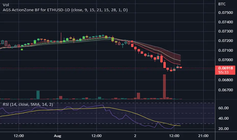
CDC ActionZone BF for ETHUSD-1D © PRoSkYNeT-EE
Based on improvements from "Kitti-Playbook Action Zone V.4.2.0.3 for Stock Market"
Based on improvements from "CDC Action Zone V3 2020 by piriya33"
Based on Triple MACD crossover between 9/15, 21/28, 15/28 for filter error signal (noise) from CDC ActionZone V3
MACDs generated from the execution of millions of times in the "Brute Force Algorithm" to backtest data from the past 5 years. ( 2017-08-21 to 2022-08-01 )
Released 2022-08-01
***** The indicator is used in the ETHUSD 1 Day period ONLY *****
Recommended Stop Loss : -4 % (execute stop Loss after candlestick has been closed)
Backtest Result ( Start $100 )
Winrate 63 % (Win:12, Loss:7, Total:19)
Live Days 1,806 days
B : Buy
S : Sell
SL : Stop Loss
2022-07-19 07 - 1,542 : B 6.971 ETH
2022-04-13 07 - 3,118 : S 8.98 % $10,750 12,7,19 63 %
2022-03-20 07 - 2,861 : B 3.448 ETH
2021-12-03 07 - 4,216 : SL -8.94 % $9,864 11,7,18 61 %
2021-11-30 07 - 4,630 : B 2.340 ETH
2021-11-18 07 - 3,997 : S 13.71 % $10,832 11,6,17 65 %
2021-10-05 07 - 3,515 : B 2.710 ETH
2021-09-20 07 - 2,977 : S 29.38 % $9,526 10,6,16 63 %
2021-07-28 07 - 2,301 : B 3.200 ETH
2021-05-20 07 - 2,769 : S 50.49 % $7,363 9,6,15 60 %
2021-03-30 07 - 1,840 : B 2.659 ETH
2021-03-22 07 - 1,681 : SL -8.29 % $4,893 8,6,14 57 %
2021-03-08 07 - 1,833 : B 2.911 ETH
2021-02-26 07 - 1,445 : S 279.27 % $5,335 8,5,13 62 %
2020-10-13 07 - 381 : B 3.692 ETH
2020-09-05 07 - 335 : S 38.43 % $1,407 7,5,12 58 %
2020-07-06 07 - 242 : B 4.199 ETH
2020-06-27 07 - 221 : S 28.49 % $1,016 6,5,11 55 %
2020-04-16 07 - 172 : B 4.598 ETH
2020-02-29 07 - 217 : S 47.62 % $791 5,5,10 50 %
2020-01-12 07 - 147 : B 3.644 ETH
2019-11-18 07 - 178 : S -2.73 % $536 4,5,9 44 %
2019-11-01 07 - 183 : B 3.010 ETH
2019-09-23 07 - 201 : SL -4.29 % $551 4,4,8 50 %
2019-09-18 07 - 210 : B 2.740 ETH
2019-07-12 07 - 275 : S 63.69 % $575 4,3,7 57 %
2019-05-03 07 - 168 : B 2.093 ETH
2019-04-28 07 - 158 : S 29.51 % $352 3,3,6 50 %
2019-02-15 07 - 122 : B 2.225 ETH
2019-01-10 07 - 125 : SL -6.02 % $271 2,3,5 40 %
2018-12-29 07 - 133 : B 2.172 ETH
2018-05-22 07 - 641 : S 5.95 % $289 2,2,4 50 %
2018-04-21 07 - 605 : B 0.451 ETH
2018-02-02 07 - 922 : S 197.42 % $273 1,2,3 33 %
2017-11-11 07 - 310 : B 0.296 ETH
2017-10-09 07 - 297 : SL -4.50 % $92 0,2,2 0 %
2017-10-07 07 - 311 : B 0.309 ETH
2017-08-22 07 - 310 : SL -4.02 % $96 0,1,1 0 %
2017-08-21 07 - 323 : B 0.310 ETH
The Lazy Trader - Index (ETF) Trend Following Robot50/150 moving average, index (ETF) trend following robot. Coded for people who cannot psychologically handle dollar-cost-averaging through bear markets and extreme drawdowns (although DCA can produce better results eventually), this robot helps you to avoid bear markets. Be a fair-weathered friend of Mr Market, and only take up his offer when the sun is shining! Designed for the lazy trader who really doesn't care...
Recommended Chart Settings:
Asset Class: ETF
Time Frame: Daily
Necessary ETF Macro Conditions:
a) Country must have healthy demographics, good ratio of young > old
b) Country population must be increasing
c) Country must be experiencing price-inflation
Default Robot Settings:
Slow Moving Average: 50 (integer) //adjust to suit your underlying index
Fast Moving Average: 150 (integer) //adjust to suit your underlying index
Bullish Slope Angle: 5 (degrees) //up angle of moving averages
Bearish Slope Angle: -5 (degrees) //down angle of moving averages
Average True Range: 14 (integer) //input for slope-angle formula
Risk: 100 (%) //100% risk means using all equity per trade
ETF Test Results (Default Settings):
SPY (1993 to 2020, 27 years), 332% profit, 20 trades, 6.4 profit factor, 7% drawdown
EWG (1996 to 2020, 24 years), 310% profit, 18 trades, 3.7 profit factor, 10% drawdown
EWH (1996 to 2020, 24 years), 4% loss, 26 trades, 0.9 profit factor, 36% drawdown
QQQ (1999 to 2020, 21 years), 232% profit, 17 trades, 3.6 profit factor, 2% drawdown
EEM (2003 to 2020, 17 years), 73% profit, 17 trades, 1.1 profit factor, 3% drawdown
GXC (2007 to 2020, 13 years), 18% profit, 14 trades, 1.3 profit factor, 26% drawdown
BKF (2009 to 2020, 11 years), 11% profit, 13 trades, 1.2 profit factor, 33% drawdown
A longer time in the markets is better, with the exception of EWH. 6 out of 7 tested ETFs were profitable, feel free to test on your favourite ETF (default settings) and comment below.
Risk Warning:
Not tested on commodities nor other financial products like currencies (code will not work), feel free to leave comments below.
Moving Average Slope Angle Formula:
Reproduced and modified from source:

BTC and ETH Long strategy - version 1I will start with a small introduction about myself. I'm now trading cryto currencies manually for almost 2 years. I decided to start after watching a documentary on the TV showing people who made big money during the Bitcoin pump which happened at the end of 2017.
The next day, I asked myself "Why should I not give it a try and learn how to trade".
This was in February 2018 and the price of Bitcoin was around 11500USD.
I didn't know how to trade. In fact, I didn't know the trading industry at all.
So, my first step into trading was to open an account with a broken. Then I directly bought 200$ worst of BTC . At that time, I saw the graph and thought "This can only go back in the upward direction!" :)
I didn't know anything about Stop loss, Take profit and Risk management.
Today, almost 2 years after, I think that I know how to trade and can also confirm that I still hold this bag of 200$ of bitcoin from 2018 :)
I did spend the 2 last years to learn technical analysis , risk management and leverage trading.
Today (14/05/2020), I know what I'm doing and I'm happy to see that the 2 last years have been positive in terms of gains. Of course, I did not make crazy money with my saving but at least I made more than if I would have kept it in my bank account.
Even if I like trading, I have a full time job which requires my full energy and lots of focus, so, the biggest problem I had is that I didn't have enough time to look at the charts.
Also, I realized that sometimes, neither technical analysis , nor fundamentals worked with crypto currency (at least for short time trading). So, as I have a developer background I decided to try to have a look at algo trading.
The goal for me was neither to make complex algos nor to beat the market but just to automate my trading with simple bot catching the big waves.
I then started to take a look at TV pine script and played with it.
I did my first LONG script in February 2020 to Long the BTC Market. It has some limitations but works well enough for me for the time being. Even if the real trades will bring me half of what the back testing shows, this will still be a lot more than what I was used to win during the last 2 years with my manual trading.
So, here we are! Below you will find some details about my first LONG script. I'm happy to share it with you.
Feel free to play with it, give your comments and bring improvements to it.
But please note that it only works fine with the candle size and crypto pair that I have mentioned below. If you use other settings this algo might loose money!
- Crypto pairs : XBTUSD and ETHXBT
- Candle size: 2 Hours
- Indicator used: Volatility , MACD (12, 26, 7), SMA (100), SMA (200), EMA (20)
- Default StopLoss: -1.5%
- Entry in position if: Volatility < 2%
AND MACD moving up
AND AME (20) moving up
AND SMA (100) moving up
AND SMA (200) moving up
AND EMA (20) > SAM (100)
AND SMA (100) > SMA (200)
- Exit the postion if: Stoploss is reached
OR EMA (20) crossUnder SMA (100)
Here is a summary of the results for this script:
XBTUSD : 01/01/2019 --> 14/05/2020 = +107%
ETHXBT : 01/01/2019 --> 14/05/2020 = +39%
ETHUSD : 01/01/2019 --> 14/05/2020 = +112%
It is far away from being perfect. There are still plenty of things which can be done to improve it but I just wanted to share it :) .
Enjoy playing with it....

Ichimoku Kinkō hyō Keizen 改MTF善The script is not finnished yet and show's an other interpretation of how it could be scripted
Step -1 is complete... Basic Ichimoku with asjutable length and editable lines colors and visibilities.
Step -2 in progress... Adding ability to une multiple Spans, sens and Kumo on higher and lower timeframe.
Your Step : Like and Share ;) have a good year 2020 !
2020-01-06 /--------/ -R.V.
Jan 06
Release Notes: The script is not finnished yet and show's an other interpretation of how it could be scripted
Step -1 is complete... Basic Ichimoku with asjutable length and editable lines colors and visibilities.
Step -2 in progress... Adding ability to une multiple Spans, sens and Kumo on higher and lower timeframe.
Your Step : Like and Share ;) have a good year 2020 !
2020-01-06 /--------/ -R.V.
Jan 07
Jan 13
Release Notes: MTF Ichimoku is on it's way !!
Jan 17
Release Notes: The script is not finnished yet and show's an interpretation of how it could be scripted
Step -1 is complete... Basic Ichimoku with asjutable length and editable lines colors and visibilities.
Step -2 in complete... Adding ability to use multiple Spans, sens and Kumo on higher timeframe.
Step -3 in progress... Creating a UNIX based function to framgments actual chart periods in subcandles or "Subprices/periods" to plot multiple Spans, sens and Kumo on LOWER timeframe.
Your Step : Like and Share ;) have a good year 2020 !
/--------Coder--------/ -R.V.

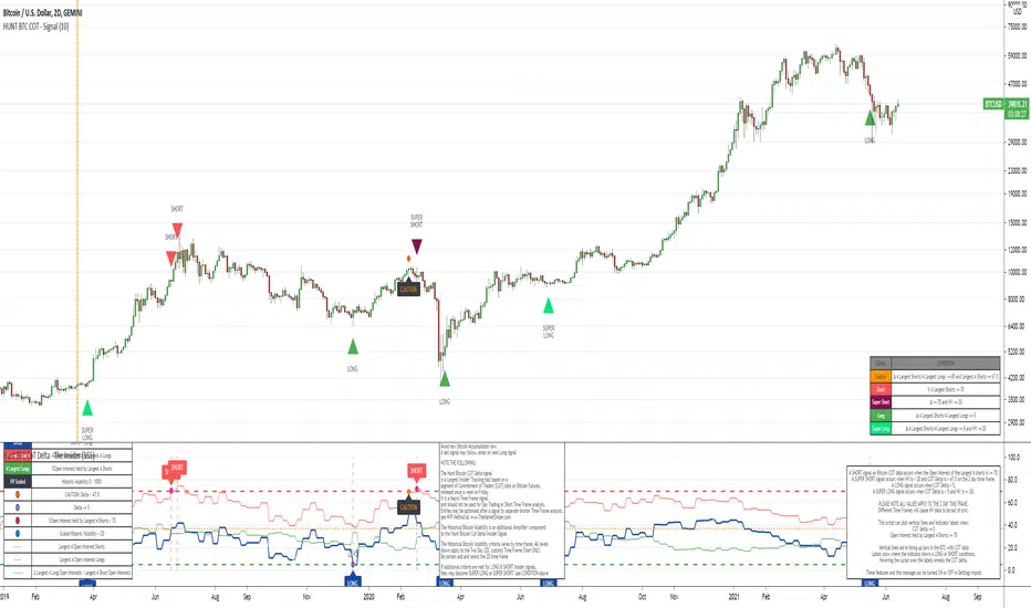
The Insider - Hunt Bitcoin CoT DeltaThe Insider - Hunt Bitcoin CoT Delta
The gift of the Squeeze in the Largest 4 open Interest Shorts vs Longs.
Why Bother another CoT signal?
Its different & focused on the Insider's.
Performance -
This Indicator provided a
1. Signal 1 = 26th March 2019 = SUPER LONG at $4,500 that saw a near $14,000 run up
2. Signal 2 = 18th & 24th June 2019 = SHORT at the second & final level $11,700 after repeated attempts & failure in the $13K range, the mini Echo Bitcoin Bull of 2019
3. Signal 3 = 17th December 2019 = LONG $6,900, Bitcoin rallied to Mid $10,500's
4. Signal 4 = 18th Feb 2020 = SUPER SHORT from $9,700's to a final extreme Low of $3,000, calling the CV-19 collapse
5. Signal 5 = 17th March 2020 = LONG from $5,400 no closure point yet
6. Signal 6 = 29th June 2020 = SUPER LONG reiterate from $10,700 no closure sell signal yet
7. Signal 7 = 17th May 2020 = LONG another accumulate LONG with no sell signal yet generated at Post H&S's low of $33,000
Note - This indicator only commences March 2019, as Bitcoin futures were a recent introduction and needed to settle for 6 months in both use and data, no signals were meaningful prior & data was light.
What is Provided. - Please note the need to also add the Hunt Bitcoin Historical Volatility Indicator for full understanding.
We provide 3 things with the 3 indicators.
'Insider' indications from Largest players in the futures market.
1. Bitcoin Macro Buy Signals.
a) The Bitcoin Commitment of Traders results see us focus solely on Largest 4 Short Open Interest & Largest 4 Long Open Interest aspects of the CoT Release data.
When the difference - is tight, a kind of pinch, these have been great Buy signals in Bitcoin.
We call this difference the Delta & When Delta is 5% or less Bitcoin is a Buy.
2. Bitcoin Macro Sells.
a) A sell signal is Triggered in Bitcoin at any point the Largest 4 short OI > or = to 70
3. AMPLIFIER Trade signals 'Super' Longs or Shorts -
Extreme low volatility events leads to highly impulsive & volatile subsequent moves, if either of 1 or 2 above occur, combined with extreme low volatility
a 'Super Long' or 'SUPER SELL' is generated. In the case of the short side, given Bitcoins general expansive and MACRO Bull trend since inception, we seek an additional component
that is an extreme differential/Delta reading between 4 biggest Longs & Shorts OI.
Namely CoT Delta also must be > 47.5%
We also have a Cautionary level, where it is not necessarily a good idea to accumulate Bitcon, as a better opportunity lower may avail itself, see conditions below.
So the required logic explicitly stated below for all Signals.
1. Long - Hunt Bitcoin CoT Delta < or = 5
2. SUPER Long - Hunt Bitcoin CoT Delta < or = 5; and 2 Day Historical Bitcoin Volatility = or < 20
3. Short - Largest 4 Sellers OI = or > 70
4. SUPER Short - Largest 4 Sellers OI = or > 70; AND..
Hunt Bitcoin CoT Delta = or > 47.5 AND 2 Day Historical BTC Volatility = or < 20
5. Caution - Largest 4 Sellers OI = or > 67.5 AND Hunt Bitcoin CoT Delta = or > 45
WARNING SEE Notes Below
Note 1 - = Largest 4 Open Interest Shorts
Note 2 - = Largest 4 Open Interest Longs
Note 3 - = Hunt Cot Delta = (Largest 4 sellers OI) -( Largest 4 Buyers OI)
Caution = Avoid new Bitcoin Accumulation Right Now, A sell signal might follow Enter on next Long
Note 4 - The Hunt Bitcoin COT Delta signal is a Largest 'Insider' Tracking tool based on a segment of Commitment of Traders data on Bitcoin Futures, released once a week on a Friday.
It is a Macro Timeframe signal , and should not be used for Day trading and Short Timeframe analysis , Entries may be optimised after a Hunt Bitcoin CoT Signal is generated by separate shorter Timeframe analysis.
Note 5 - The Historical Bitcoin Volatility is an additional 'Amplifier' component to the 'Hunt Bitcoin Cot Delta' Insider Signal
Note 6 - The Historical Bitcoin Volatility criteria varies by timeframe, the above levels are those applying on a Two Day TF Chart, select this custom timeframe in Trading View.
if additional criteria are met for LONG & SHORT insider signals, they may become 'Super Longs/Shorts', see conditions box above.
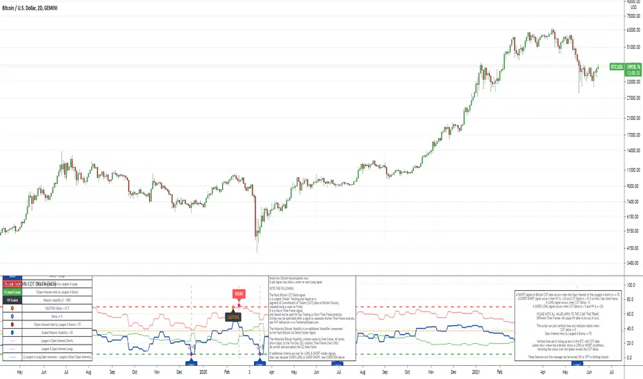
The Signal - Hunt Bitcoin CoT Buy/SellThe Signal - Hunt Bitcoin CoT Buy/Sell
Why Bother with another CoT signal?
Its different & focused on the Insider's. The Largest 4 Open Interest Seller and the Largest 4 open Interest Longs, plus the distance they are apart, the Delta, what does high percentage of Largest 4 sellers mean with a low 4 OI Buyers. , what when the usually higher Sellers are low and the largest 4 buyers almost the same value , Time to track the insiders Delta..
Performance -
This Indicator provided a
1. Signal 1 = 26th March 2019 = SUPER LONG at $4,500 that saw a near $14,000 run up
2. Signal 2 = 18th & 24th June 2019 = SHORT at the second & final level $11,700 after repeated attempts & failure in the $13K range, the mini Echo Bitcoin Bull of 2019
3. Signal 3 = 17th December 2019 = LONG $6,900, Bitcoin rallied to Mid $10,500's
4. Signal 4 = 18th Feb 2020 = SUPER SHORT from $9,700's to a final extreme Low of $3,000, calling the CV-19 collapse
5. Signal 5 = 17th March 2020 = LONG from $5,400 no closure point yet
6. Signal 6 = 29th June 2020 = SUPER LONG reiterate from $10,700 no closure sell signal yet
7. Signal 7 = 17th May 2020 = LONG another accumulate LONG with no sell signal yet generated at Post H&S's low of $33,000
Note - This indicator only commences March 2019, as Bitcoin futures were a recent introduction and needed to settle for 6 months in both use and data, no signals were meaningful prior & data was light.
What is Provided. - Please note the need to also add the Hunt Bitcoin Historical Volatility Indicator for full understanding.
We provide 3 things with the 3 indicators.
'Insider' indications from Largest players in the futures market.
1. Bitcoin Macro Buy Signals.
a) The Bitcoin Commitment of Traders results see us focus solely on Largest 4 Short Open Interest & Largest 4 Long Open Interest aspects of the CoT Release data.
When the difference - is tight, a kind of pinch, these have been great Buy signals in Bitcoin.
We call this difference the Delta & When Delta is 5% or less Bitcoin is a Buy.
2. Bitcoin Macro Sells.
a) A sell signal is Triggered in Bitcoin at any point the Largest 4 short OI > or = to 70
3. AMPLIFIER Trade signals 'Super' Longs or Shorts -
Extreme low volatility events leads to highly impulsive & volatile subsequent moves, if either of 1 or 2 above occur, combined with extreme low volatility
a 'Super Long' or 'SUPER SELL' is generated. In the case of the short side, given Bitcoins general expansive and MACRO Bull trend since inception, we seek an additional component
that is an extreme differential/Delta reading between 4 biggest Longs & Shorts OI.
Namely CoT Delta also must be > 47.5%
We also have a Cautionary level, where it is not necessarily a good idea to accumulate Bitcon, as a better opportunity lower may avail itself, see conditions below.
So the required logic explicitly stated below for all Signals.
1. Long - Hunt Bitcoin CoT Delta < or = 5
2. SUPER Long - Hunt Bitcoin CoT Delta < or = 5; and 2 Day Historical Bitcoin Volatility = or < 20
3. Short - Largest 4 Sellers OI = or > 70
4. SUPER Short - Largest 4 Sellers OI = or > 70; AND..
Hunt Bitcoin CoT Delta = or > 47.5 AND 2 Day Historical BTC Volatility = or < 20
5. Caution - Largest 4 Sellers OI = or > 67.5 AND Hunt Bitcoin CoT Delta = or > 45
WARNING SEE Notes Below
Note 1 - = Largest 4 Open Interest Shorts
Note 2 - = Largest 4 Open Interest Longs
Note 3 - = Hunt Cot Delta = (Largest 4 sellers OI) -( Largest 4 Buyers OI)
Caution = Avoid new Bitcoin Accumulation Right Now, A sell signal might follow Enter on next Long
Note 4 - The Hunt Bitcoin COT Delta signal is a Largest 'Insider' Tracking tool based on a segment of Commitment of Traders data on Bitcoin Futures, released once a week on a Friday.
It is a Macro Timeframe signal , and should not be used for Day trading and Short Timeframe analysis , Entries may be optimised after a Hunt Bitcoin CoT Signal is generated by separate shorter Timeframe analysis.
Note 5 - The Historical Bitcoin Volatility is an additional 'Amplifier' component to the 'Hunt Bitcoin Cot Delta' Insider Signal
Note 6 - The Historical Bitcoin Volatility criteria varies by timeframe, the above levels are those applying on a Two Day TF Chart, select this custom timeframe in Trading View.
if additional criteria are met for LONG & SHORT insider signals, they may become 'Super Longs/Shorts', see conditions box above.

The Amplifier - Two Day Historical Bitcoin Volatility PlotThe 3rd piece to the other two pieces to our CoT study. This is the Amplifier, which turns select signals into 'Super' Buys/Sells
The other two being the 'Bitcoin Insider CoT Delta', and the on chart Price indicator most will have, if no others the 'Hunt Bitcoin CoT Buy/Sell Signals' that will indicate the key signals, ave 4 a year on the chart as they occur.
Why Bother another CoT signal?
Its different & focused on the Insider's.
Performance -
This Indicator provided a
1. Signal 1 = 26th March 2019 = SUPER LONG at $4,500 that saw a near $14,000 run up
2. Signal 2 = 18th & 24th June 2019 = SHORT at the second & final level $11,700 after repeated attempts & failure in the $13K range, the mini Echo Bitcoin Bull of 2019
3. Signal 3 = 17th December 2019 = LONG $6,900, Bitcoin rallied to Mid $10,500's
4. Signal 4 = 18th Feb 2020 = SUPER SHORT from $9,700's to a final extreme Low of $3,000, calling the CV-19 collapse
5. Signal 5 = 17th March 2020 = LONG from $5,400 no closure point yet
6. Signal 6 = 29th June 2020 = SUPER LONG reiterate from $10,700 no closure sell signal yet
7. Signal 7 = 17th May 2020 = LONG another accumulate LONG with no sell signal yet generated at Post H&S's low of $33,000
Note - This indicator only commences March 2019, as Bitcoin futures were a recent introduction and needed to settle for 6 months in both use and data, no signals were meaningful prior & data was light.
What is Provided. - Please note the need to also add the Hunt Bitcoin Historical Volatility Indicator for full understanding.
We provide 3 things with the 3 indicators.
'Insider' indications from Largest players in the futures market.
1. Bitcoin Macro Buy Signals.
a) The Bitcoin Commitment of Traders results see us focus solely on Largest 4 Short Open Interest & Largest 4 Long Open Interest aspects of the CoT Release data.
When the difference - is tight, a kind of pinch, these have been great Buy signals in Bitcoin.
We call this difference the Delta & When Delta is 5% or less Bitcoin is a Buy.
2. Bitcoin Macro Sells.
a) A sell signal is Triggered in Bitcoin at any point the Largest 4 short OI > or = to 70
3. AMPLIFIER Trade signals 'Super' Longs or Shorts -
Extreme low volatility events leads to highly impulsive & volatile subsequent moves, if either of 1 or 2 above occur, combined with extreme low volatility
a 'Super Long' or 'SUPER SELL' is generated. In the case of the short side, given Bitcoins general expansive and MACRO Bull trend since inception, we seek an additional component
that is an extreme differential/Delta reading between 4 biggest Longs & Shorts OI.
Namely CoT Delta also must be > 47.5%
We also have a Cautionary level, where it is not necessarily a good idea to accumulate Bitcon, as a better opportunity lower may avail itself, see conditions below.
So the required logic explicitly stated below for all Signals.
1. Long - Hunt Bitcoin CoT Delta < or = 5
2. SUPER Long - Hunt Bitcoin CoT Delta < or = 5; and 2 Day Historical Bitcoin Volatility = or < 20
3. Short - Largest 4 Sellers OI = or > 70
4. SUPER Short - Largest 4 Sellers OI = or > 70; AND..
Hunt Bitcoin CoT Delta = or > 47.5 AND 2 Day Historical BTC Volatility = or < 20
5. Caution - Largest 4 Sellers OI = or > 67.5 AND Hunt Bitcoin CoT Delta = or > 45
WARNING SEE Notes Below
Note 1 - = Largest 4 Open Interest Shorts
Note 2 - = Largest 4 Open Interest Longs
Note 3 - = Hunt Cot Delta = (Largest 4 sellers OI) -( Largest 4 Buyers OI)
Caution = Avoid new Bitcoin Accumulation Right Now, A sell signal might follow Enter on next Long
Note 4 - The Hunt Bitcoin COT Delta signal is a Largest 'Insider' Tracking tool based on a segment of Commitment of Traders data on Bitcoin Futures, released once a week on a Friday.
It is a Macro Timeframe signal , and should not be used for Day trading and Short Timeframe analysis , Entries may be optimised after a Hunt Bitcoin CoT Signal is generated by separate shorter Timeframe analysis.
Note 5 - The Historical Bitcoin Volatility is an additional 'Amplifier' component to the 'Hunt Bitcoin Cot Delta' Insider Signal
Note 6 - The Historical Bitcoin Volatility criteria varies by timeframe, the above levels are those applying on a Two Day TF Chart, select this custom timeframe in Trading View.
if additional criteria are met for LONG & SHORT insider signals, they may become 'Super Longs/Shorts', see conditions box above.

Hunt Bitcoin CoT Buy/Sell signalWhy Bother another CoT signal?
Its different & focused on the Insider's.
Performance -
This Indicator provided a
1. Signal 1 = 26th March 2019 = SUPER LONG at $4,500 that saw a near $14,000 run up
2. Signal 2 = 18th & 24th June 2019 = SHORT at the second & final level $11,700 after repeated attempts & failure in the $13K range, the mini Echo Bitcoin Bull of 2019
3. Signal 3 = 17th December 2019 = LONG $6,900, Bitcoin rallied to Mid $10,500's
4. Signal 4 = 18th Feb 2020 = SUPER SHORT from $9,700's to a final extreme Low of $3,000, calling the CV-19 collapse
5. Signal 5 = 17th March 2020 = LONG from $5,400 no closure point yet
6. Signal 6 = 29th June 2020 = SUPER LONG reiterate from $10,700 no closure sell signal yet
7. Signal 7 = 17th May 2020 = LONG another accumulate LONG with no sell signal yet generated at Post H&S's low of $33,000
Note - This indicator only commences March 2019, as Bitcoin futures were a recent introduction and needed to settle for 6 months in both use and data, no signals were meaningful prior & data was light.
What is Provided. - Please note the need to also add the Hunt Bitcoin Historical Volatility Indicator for full understanding.
We provide 3 things with the 3 indicators.
'Insider' indications from Largest players in the futures market.
1. Bitcoin Macro Buy Signals.
a) The Bitcoin Commitment of Traders results see us focus solely on Largest 4 Short Open Interest & Largest 4 Long Open Interest aspects of the CoT Release data.
When the difference - is tight, a kind of pinch, these have been great Buy signals in Bitcoin.
We call this difference the Delta & When Delta is 5% or less Bitcoin is a Buy.
2. Bitcoin Macro Sells.
a) A sell signal is Triggered in Bitcoin at any point the Largest 4 short OI > or = to 70
3. AMPLIFIER Trade signals 'Super' Longs or Shorts -
Extreme low volatility events leads to highly impulsive & volatile subsequent moves, if either of 1 or 2 above occur, combined with extreme low volatility
a 'Super Long' or 'SUPER SELL' is generated. In the case of the short side, given Bitcoins general expansive and MACRO Bull trend since inception, we seek an additional component
that is an extreme differential/Delta reading between 4 biggest Longs & Shorts OI.
Namely CoT Delta also must be > 47.5%
We also have a Cautionary level, where it is not necessarily a good idea to accumulate Bitcon, as a better opportunity lower may avail itself, see conditions below.
So the required logic explicitly stated below for all Signals.
1. Long - Hunt Bitcoin CoT Delta < or = 5
2. SUPER Long - Hunt Bitcoin CoT Delta < or = 5; and 2 Day Historical Bitcoin Volatility = or < 20
3. Short - Largest 4 Sellers OI = or > 70
4. SUPER Short - Largest 4 Sellers OI = or > 70; AND..
Hunt Bitcoin CoT Delta = or > 47.5 AND 2 Day Historical BTC Volatility = or < 20
5. Caution - Largest 4 Sellers OI = or > 67.5 AND Hunt Bitcoin CoT Delta = or > 45
WARNING SEE Notes Below
Note 1 - = Largest 4 Open Interest Shorts
Note 2 - = Largest 4 Open Interest Longs
Note 3 - = Hunt Cot Delta = (Largest 4 sellers OI) -( Largest 4 Buyers OI)
Caution = Avoid new Bitcoin Accumulation Right Now, A sell signal might follow Enter on next Long
Note 4 - The Hunt Bitcoin COT Delta signal is a Largest 'Insider' Tracking tool based on a segment of Commitment of Traders data on Bitcoin Futures, released once a week on a Friday.
It is a Macro Timeframe signal , and should not be used for Day trading and Short Timeframe analysis , Entries may be optimised after a Hunt Bitcoin CoT Signal is generated by separate shorter Timeframe analysis.
Note 5 - The Historical Bitcoin Volatility is an additional 'Amplifier' component to the 'Hunt Bitcoin Cot Delta' Insider Signal
Note 6 - The Historical Bitcoin Volatility criteria varies by timeframe, the above levels are those applying on a Two Day TF Chart, select this custom timeframe in Trading View.
if additional criteria are met for LONG & SHORT insider signals, they may become 'Super Longs/Shorts', see conditions box above.

Hunt Bitcoin CoT Open Interest DeltaWhy Bother another CoT signal?
Its different & focused on the Insider's.
Performance -
This Indicator provided a
1. Signal 1 = 26th March 2019 = SUPER LONG at $4,500 that saw a near $14,000 run up
2. Signal 2 = 18th & 24th June 2019 = SHORT at the second & final level $11,700 after repeated attempts & failure in the $13K range, the mini Echo Bitcoin Bull of 2019
3. Signal 3 = 17th December 2019 = LONG $6,900, Bitcoin rallied to Mid $10,500's
4. Signal 4 = 18th Feb 2020 = SUPER SHORT from $9,700's to a final extreme Low of $3,000, calling the CV-19 collapse
5. Signal 5 = 17th March 2020 = LONG from $5,400 no closure point yet
6. Signal 6 = 29th June 2020 = SUPER LONG reiterate from $10,700 no closure sell signal yet
7. Signal 7 = 17th May 2020 = LONG another accumulate LONG with no sell signal yet generated at Post H&S's low of $33,000
Note - This indicator only commences March 2019, as Bitcoin futures were a recent introduction and needed to settle for 6 months in both use and data, no signals were meaningful prior & data was light.
What is Provided. - Please note the need to also add the Hunt Bitcoin Historical Volatility Indicator for full understanding.
We provide 3 things with the 3 indicators.
'Insider' indications from Largest players in the futures market.
1. Bitcoin Macro Buy Signals.
a) The Bitcoin Commitment of Traders results see us focus solely on Largest 4 Short Open Interest & Largest 4 Long Open Interest aspects of the CoT Release data.
When the difference - is tight, a kind of pinch, these have been great Buy signals in Bitcoin.
We call this difference the Delta & When Delta is 5% or less Bitcoin is a Buy.
2. Bitcoin Macro Sells.
a) A sell signal is Triggered in Bitcoin at any point the Largest 4 short OI > or = to 70
3. AMPLIFIER Trade signals 'Super' Longs or Shorts -
Extreme low volatility events leads to highly impulsive & volatile subsequent moves, if either of 1 or 2 above occur, combined with extreme low volatility
a 'Super Long' or 'SUPER SELL' is generated. In the case of the short side, given Bitcoins general expansive and MACRO Bull trend since inception, we seek an additional component
that is an extreme differential/Delta reading between 4 biggest Longs & Shorts OI.
Namely CoT Delta also must be > 47.5%
We also have a Cautionary level, where it is not necessarily a good idea to accumulate Bitcon, as a better opportunity lower may avail itself, see conditions below.
So the required logic explicitly stated below for all Signals.
1. Long - Hunt Bitcoin CoT Delta < or = 5
2. SUPER Long - Hunt Bitcoin CoT Delta < or = 5; and 2 Day Historical Bitcoin Volatility = or < 20
3. Short - Largest 4 Sellers OI = or > 70
4. SUPER Short - Largest 4 Sellers OI = or > 70; AND..
Hunt Bitcoin CoT Delta = or > 47.5 AND 2 Day Historical BTC Volatility = or < 20
5. Caution - Largest 4 Sellers OI = or > 67.5 AND Hunt Bitcoin CoT Delta = or > 45
WARNING SEE Notes Below
Note 1 - = Largest 4 Open Interest Shorts
Note 2 - = Largest 4 Open Interest Longs
Note 3 - = Hunt Cot Delta = (Largest 4 sellers OI) -( Largest 4 Buyers OI)
Caution = Avoid new Bitcoin Accumulation Right Now, A sell signal might follow Enter on next Long
Note 4 - The Hunt Bitcoin COT Delta signal is a Largest 'Insider' Tracking tool based on a segment of Commitment of Traders data on Bitcoin Futures, released once a week on a Friday.
It is a Macro Timeframe signal , and should not be used for Day trading and Short Timeframe analysis , Entries may be optimised after a Hunt Bitcoin CoT Signal is generated by separate shorter Timeframe analysis.
Note 5 - The Historical Bitcoin Volatility is an additional 'Amplifier' component to the 'Hunt Bitcoin Cot Delta' Insider Signal
Note 6 - The Historical Bitcoin Volatility criteria varies by timeframe, the above levels are those applying on a Two Day TF Chart, select this custom timeframe in Trading View.
if additional criteria are met for LONG & SHORT insider signals, they may become 'Super Longs/Shorts', see conditions box above.
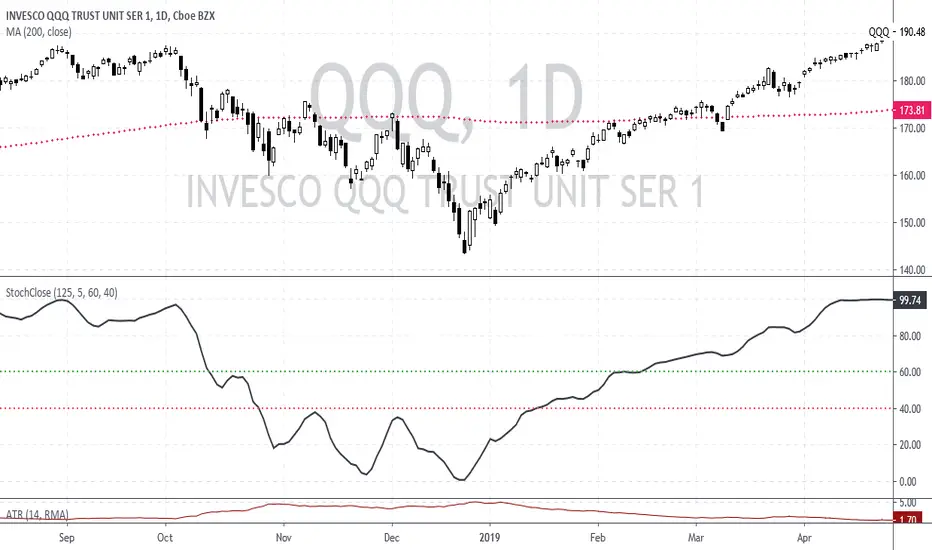
Stochastic based on Closing Prices - Identify and Rank TrendsStochClose is a trend indicator that can be used on its own to measure trend strength, in a scan to rank a group of securities according to trend strength or as part of a trend following strategy. Moreover, it acts as a volatility-adjusted trend indicator that puts securities on an equal footing.
StochClose measures the location of the current close relative to the close-only high-low range over a given period of time. In contrast to the traditional Stochastic Oscillator, this indicator only uses closing prices. Traditional Stochastic uses intraday highs and lows to calculate the range. The focus on closing prices reduces signal noise caused by intraday highs and lows, and filters out errant or irrationally exuberant price spikes.
Here are some examples when the high or low was out of proportion and suspect. Perhaps most famously, there were errant spike lows in dozens of ETFs in August 2015 (XLK, IJR, ITB). There were other spikes in VMBS (October 2014), IJR (October 2008) and KRE (May 2011). Elsewhere, there were suspicious spikes in IEI (April 2020), CHD (March 2020), CCRN (March 2020) and FNB (March 2020)
The preferred setting to identify medium and long-term uptrends is 125 days with 5 days smoothing. 125 days covers around six months. Thus, StochClose(125,5) is a 5-day SMA of the 125-day Stochastic based on closing prices. Smoothing with the 5-day SMA introduces a little lag, but reduces whipsaws and signal noise.
StochClose fluctuates between 0 and 100 with 50 as the midpoint. Values above 80 indicate that the current price is near the high end of the 125-day range, while values below 20 indicate that price is near the low end of the range. For signals, a move above 60 puts the indicator firmly in the top half of the range and points to an uptrend. A move below 40 puts the indicator firmly in the bottom half of the range and points to a downtrend.
StochClose values can also be ranked to separate the leaders from the laggards. In contrast to Rate-of-Change and Percentage Above/Below a Moving Average, StochClose acts as a volatility-adjusted indicator that can identify trend strength or weakness. The Consumer Staples SPDR is unlikely to win in a Rate-of-Change contest with the Technology SPDR. However, it is just as easy for the Consumer Staples SPDR to get in the top of its range as it is for the Technology SPDR. StochClose puts securities on an equal footing.
StochClose measures trend direction and trend strength with one number. The indicator value tells us immediately if the security is trending higher or lower. Furthermore, we can compare this value against the values for other securities. Securities with higher StochClose values are stronger than those with lower values.
COT IndexTHE HIDDEN INTELLIGENCE IN FUTURES MARKETS
What if you could see what the smartest players in the futures markets are doing before the crowd catches on? While retail traders chase momentum indicators and moving averages, obsess over Japanese candlestick patterns, and debate whether the RSI should be set to fourteen or twenty-one periods, institutional players leave footprints in the sand through their mandatory reporting to the Commodity Futures Trading Commission. These footprints, published weekly in the Commitment of Traders reports, have been hiding in plain sight for decades, available to anyone with an internet connection, yet remarkably few traders understand how to interpret them correctly. The COT Index indicator transforms this raw institutional positioning data into actionable trading signals, bringing Wall Street intelligence to your trading screen without requiring expensive Bloomberg terminals or insider connections.
The uncomfortable truth is this: Most retail traders operate in a binary world. Long or short. Buy or sell. They apply technical analysis to individual positions, constrained by limited capital that forces them to concentrate risk in single directional bets. Meanwhile, institutional traders operate in an entirely different dimension. They manage portfolios dynamically weighted across multiple markets, adjusting exposure based on evolving market conditions, correlation shifts, and risk assessments that retail traders never see. A hedge fund might be simultaneously long gold, short oil, neutral on copper, and overweight agricultural commodities, with position sizes calibrated to volatility and portfolio Greeks. When they increase gold exposure from five percent to eight percent of portfolio allocation, this rebalancing decision reflects sophisticated analysis of opportunity cost, risk parity, and cross-market dynamics that no individual chart pattern can capture.
This portfolio reweighting activity, multiplied across hundreds of institutional participants, manifests in the aggregate positioning data published weekly by the CFTC. The Commitment of Traders report does not show individual trades or strategies. It shows the collective footprint of how actual commercial hedgers and large speculators have allocated their capital across different markets. When mining companies collectively increase forward gold sales to hedge thirty percent more production than last quarter, they are not reacting to a moving average crossover. They are making strategic allocation decisions based on production forecasts, cost structures, and price expectations derived from operational realities invisible to outside observers. This is portfolio management in action, revealed through positioning data rather than price charts.
If you want to understand how institutional capital actually flows, how sophisticated traders genuinely position themselves across market cycles, the COT report provides a rare window into that hidden world. But understand what you are getting into. This is not a tool for scalpers seeking confirmation of the next five-minute move. This is not an oscillator that flashes oversold at market bottoms with convenient precision. COT analysis operates on a timescale measured in weeks and months, revealing positioning shifts that precede major market turns but offer no precision timing. The data arrives three days stale, published only once per week, capturing strategic positioning rather than tactical entries.
If you need instant gratification, if you trade intraday moves, if you demand mechanical signals with ninety percent accuracy, close this document now. COT analysis rewards patience, position sizing discipline, and tolerance for being early. It punishes impatience, overleveraging, and the expectation that any single indicator can substitute for market understanding.
The premise is deceptively simple. Every Tuesday, large traders in futures markets must report their positions to the CFTC. By Friday afternoon, this data becomes public. Academic research spanning three decades has consistently shown that not all market participants are created equal. Some traders consistently profit while others consistently lose. Some anticipate major turning points while others chase trends into exhaustion. Bessembinder and Chan (1992) demonstrated in their seminal study that commercial hedgers, those with actual exposure to the underlying commodity or financial instrument, possess superior forecasting ability compared to speculators. Their research, published in the Journal of Finance, found statistically significant predictive power in commercial positioning, particularly at extreme levels. This finding challenged the efficient market hypothesis and opened the door to a new approach to market analysis based on positioning rather than price alone.
Think about what this means. Every week, the government publishes a report showing you exactly how the most informed market participants are positioned. Not their opinions. Not their predictions. Their actual money at risk. When agricultural producers collectively hold their largest short hedge in five years, they are not making idle speculation. They are locking in prices for crops they will harvest, informed by private knowledge of weather conditions, soil quality, inventory levels, and demand expectations invisible to outside observers. When energy companies aggressively hedge forward production at current prices, they reveal information about expected supply that no analyst report can capture. This is not technical analysis based on past prices. This is not fundamental analysis based on publicly available data. This is behavioral analysis based on how the smartest money is actually positioned, how institutions allocate capital across portfolios, and how those allocation decisions shift as market conditions evolve.
WHY SOME TRADERS KNOW MORE THAN OTHERS
Building on this foundation, Sanders, Boris and Manfredo (2004) conducted extensive research examining the behaviour patterns of different trader categories. Their work, which analyzed over a decade of COT data across multiple commodity markets, revealed a fascinating dynamic that challenges much of what retail traders are taught. Commercial hedgers consistently positioned themselves against market extremes, buying when speculators were most bearish and selling when speculators reached peak bullishness. The contrarian positioning of commercials was not random noise but rather reflected their superior information about supply and demand fundamentals. Meanwhile, large speculators, primarily hedge funds and commodity trading advisors, exhibited strong trend-following behaviour that often amplified market moves beyond fundamental values. Small traders, the retail participants, consistently entered positions late in trends, frequently near turning points, making them reliable contrary indicators.
Wang (2003) extended this research by demonstrating that the predictive power of commercial positioning varies significantly across different commodity sectors. His analysis of agricultural commodities showed particularly strong forecasting ability, with commercial net positions explaining up to fifteen percent of return variance in subsequent weeks. This finding suggests that the informational advantages of hedgers are most pronounced in markets where physical supply and demand fundamentals dominate, as opposed to purely financial markets where information asymmetries are smaller. When a corn farmer hedges six months of expected harvest, that decision incorporates private observations about rainfall patterns, crop health, pest pressure, and local storage capacity that no distant analyst can match. When an oil refinery hedges crude oil purchases and gasoline sales simultaneously, the spread relationships reveal expectations about refining margins that reflect operational realities invisible in public data.
The theoretical mechanism underlying these empirical patterns relates to information asymmetry and different participant motivations. Commercial hedgers engage in futures markets not for speculative profit but to manage business risks. An agricultural producer selling forward six months of expected harvest is not making a bet on price direction but rather locking in revenue to facilitate financial planning and ensure business viability. However, this hedging activity necessarily incorporates private information about expected supply, inventory levels, weather conditions, and demand trends that the hedger observes through their commercial operations (Irwin and Sanders, 2012). When aggregated across many participants, this private information manifests in collective positioning.
Consider a gold mining company deciding how much forward production to hedge. Management must estimate ore grades, recovery rates, production costs, equipment reliability, labor availability, and dozens of other operational variables that determine whether locking in prices at current levels makes business sense. If the industry collectively hedges more aggressively than usual, it suggests either exceptional production expectations or concern about sustaining current price levels or combination of both. Either way, this positioning reveals information unavailable to speculators analyzing price charts and economic data. The hedger sees the physical reality behind the financial abstraction.
Large speculators operate under entirely different incentives and constraints. Commodity Trading Advisors managing billions in assets typically employ systematic, trend-following strategies that respond to price momentum rather than fundamental supply and demand. When crude oil rallies from sixty dollars to seventy dollars per barrel, these systems generate buy signals. As the rally continues to eighty dollars, position sizes increase. The strategy works brilliantly during sustained trends but becomes a liability at reversals. By the time oil reaches ninety dollars, trend-following funds are maximally long, having accumulated positions progressively throughout the rally. At this point, they represent not smart money anticipating further gains but rather crowded money vulnerable to reversal. Sanders, Boris and Manfredo (2004) documented this pattern across multiple energy markets, showing that extreme speculator positioning typically marked late-stage trend exhaustion rather than early-stage trend development.
Small traders, the retail participants who fall below reporting thresholds, display the weakest forecasting ability. Wang (2003) found that small trader positioning exhibited negative correlation with subsequent returns, meaning their aggregate positioning served as a reliable contrary indicator. The explanation combines several factors. Retail traders often lack the capital reserves to weather normal market volatility, leading to premature exits from positions that would eventually prove profitable. They tend to receive information through slower channels, entering trends after mainstream media coverage when institutional participants are preparing to exit. Perhaps most importantly, they trade with emotion, buying into euphoria and selling into panic at precisely the wrong times.
At major turning points, the three groups often position opposite each other with commercials extremely bearish, large speculators extremely bullish, and small traders piling into longs at the last moment. These high-divergence environments frequently precede increased volatility and trend reversals. The insiders with business exposure quietly exit as the momentum traders hit maximum capacity and retail enthusiasm peaks. Within weeks, the reversal begins, and positions unwind in the opposite sequence.
FROM RAW DATA TO ACTIONABLE SIGNALS
The COT Index indicator operationalizes these academic findings into a practical trading tool accessible through TradingView. At its core, the indicator normalizes net positioning data onto a zero to one hundred scale, creating what we call the COT Index. This normalization is critical because absolute position sizes vary dramatically across different futures contracts and over time. A commercial trader holding fifty thousand contracts net long in crude oil might be extremely bullish by historical standards, or it might be quite neutral depending on the context of total market size and historical ranges. Raw position numbers mean nothing without context. The COT Index solves this problem by calculating where current positioning stands relative to its range over a specified lookback period, typically two hundred fifty-two weeks or approximately five years of weekly data.
The mathematical transformation follows the methodology originally popularized by legendary trader Larry Williams, though the underlying concept appears in statistical normalization techniques across many fields. For any given trader category, we calculate the highest and lowest net position values over the lookback period, establishing the historical range for that specific market and trader group. Current positioning is then expressed as a percentage of this range, where zero represents the most bearish positioning ever seen in the lookback window and one hundred represents the most bullish extreme. A reading of fifty indicates positioning exactly in the middle of the historical range, suggesting neither extreme optimism nor pessimism relative to recent history (Williams and Noseworthy, 2009).
This index-based approach allows for meaningful comparison across different markets and time periods, overcoming the scaling problems inherent in analyzing raw position data. A commercial index reading of eighty-five in gold carries the same interpretive meaning as an eighty-five reading in wheat or crude oil, even though the absolute position sizes differ by orders of magnitude. This standardization enables systematic analysis across entire futures portfolios rather than requiring market-specific expertise for each contract.
The lookback period selection involves a fundamental tradeoff between responsiveness and stability. Shorter lookback periods, perhaps one hundred twenty-six weeks or approximately two and a half years, make the index more sensitive to recent positioning changes. However, it also increases noise and produces more false signals. Longer lookback periods, perhaps five hundred weeks or approximately ten years, create smoother readings that filter short-term noise but become slower to recognize regime changes. The indicator settings allow users to adjust this parameter based on their trading timeframe, risk tolerance, and market characteristics.
UNDERSTANDING CFTC DATA STRUCTURES
The indicator supports both Legacy and Disaggregated COT report formats, reflecting the evolution of CFTC reporting standards over decades of market development. Legacy reports categorize market participants into three broad groups: commercial traders (hedgers with underlying business exposure), non-commercial traders (large speculators seeking profit without commercial interest), and non-reportable traders (small speculators below reporting thresholds). Each category brings distinct motivations and information advantages to the market (CFTC, 2020).
The Disaggregated reports, introduced in September 2009 for physical commodity markets, provide finer granularity by splitting participants into five categories (CFTC, 2009). Producer and merchant positions capture those actually producing, processing, or merchandising the physical commodity. Swap dealers represent financial intermediaries facilitating derivative transactions for clients. Managed money includes commodity trading advisors and hedge funds executing systematic or discretionary strategies. Other reportables encompasses diverse participants not fitting the main categories. Small traders remain as the fifth group, representing retail participation.
This enhanced categorization reveals nuances invisible in Legacy reports, particularly distinguishing between different types of institutional capital and their distinct behavioural patterns. The indicator automatically detects which report type is appropriate for each futures contract and adjusts the display accordingly.
Importantly, Disaggregated reports exist only for physical commodity futures. Agricultural commodities like corn, wheat, and soybeans have Disaggregated reports because clear producer, merchant, and swap dealer categories exist. Energy commodities like crude oil and natural gas similarly have well-defined commercial hedger categories. Metals including gold, silver, and copper also receive Disaggregated treatment (CFTC, 2009). However, financial futures such as equity index futures, Treasury bond futures, and currency futures remain available only in Legacy format. The CFTC has indicated no plans to extend Disaggregated reporting to financial futures due to different market structures and participant categories in these instruments (CFTC, 2020).
THE BEHAVIORAL FOUNDATION
Understanding which trader perspective to follow requires appreciation of their distinct trading styles, success rates, and psychological profiles. Commercial hedgers exhibit anticyclical behaviour rooted in their fundamental knowledge and business imperatives. When agricultural producers hedge forward sales during harvest season, they are not speculating on price direction but rather locking in revenue for crops they will harvest. Their business requires converting volatile commodity exposure into predictable cash flows to facilitate planning and ensure survival through difficult periods. Yet their aggregate positioning reveals valuable information because these hedging decisions incorporate private information about supply conditions, inventory levels, weather observations, and demand expectations that hedgers observe through their commercial operations (Bessembinder and Chan, 1992).
Consider a practical example from energy markets. Major oil companies continuously hedge portions of forward production based on price levels, operational costs, and financial planning needs. When crude oil trades at ninety dollars per barrel, they might aggressively hedge the next twelve months of production, locking in prices that provide comfortable profit margins above their extraction costs. This hedging appears as short positioning in COT reports. If oil rallies further to one hundred dollars, they hedge even more aggressively, viewing these prices as exceptional opportunities to secure revenue. Their short positioning grows increasingly extreme. To an outside observer watching only price charts, the rally suggests bullishness. But the commercial positioning reveals that the actual producers of oil find these prices attractive enough to lock in years of sales, suggesting skepticism about sustaining even higher levels. When the eventual reversal occurs and oil declines back to eighty dollars, the commercials who hedged at ninety and one hundred dollars profit while speculators who chased the rally suffer losses.
Large speculators or managed money traders operate under entirely different incentives and constraints. Their systematic, momentum-driven strategies mean they amplify existing trends rather than anticipate reversals. Trend-following systems, the most common approach among large speculators, by definition require confirmation of trend through price momentum before entering positions (Sanders, Boris and Manfredo, 2004). When crude oil rallies from sixty dollars to eighty dollars per barrel over several months, trend-following algorithms generate buy signals based on moving average crossovers, breakouts, and other momentum indicators. As the rally continues, position sizes increase according to the systematic rules.
However, this approach becomes a liability at turning points. By the time oil reaches ninety dollars after a sustained rally, trend-following funds are maximally long, having accumulated positions progressively throughout the move. At this point, their positioning does not predict continued strength. Rather, it often marks late-stage trend exhaustion. The psychological and mechanical explanation is straightforward. Trend followers by definition chase price momentum, entering positions after trends establish rather than anticipating them. Eventually, they become fully invested just as the trend nears completion, leaving no incremental buying power to sustain the rally. When the first signs of reversal appear, systematic stops trigger, creating a cascade of selling that accelerates the downturn.
Small traders consistently display the weakest track record across academic studies. Wang (2003) found that small trader positioning exhibited negative correlation with subsequent returns in his analysis across multiple commodity markets. This result means that whatever small traders collectively do, the opposite typically proves profitable. The explanation for small trader underperformance combines several factors documented in behavioral finance literature. Retail traders often lack the capital reserves to weather normal market volatility, leading to premature exits from positions that would eventually prove profitable. They tend to receive information through slower channels, learning about commodity trends through mainstream media coverage that arrives after institutional participants have already positioned. Perhaps most importantly, retail traders are more susceptible to emotional decision-making, buying into euphoria and selling into panic at precisely the wrong times (Tharp, 2008).
SETTINGS, THRESHOLDS, AND SIGNAL GENERATION
The practical implementation of the COT Index requires understanding several key features and settings that users can adjust to match their trading style, timeframe, and risk tolerance. The lookback period determines the time window for calculating historical ranges. The default setting of two hundred fifty-two bars represents approximately one year on daily charts or five years on weekly charts, balancing responsiveness with stability. Conservative traders seeking only the most extreme, highest-probability signals might extend the lookback to five hundred bars or more. Aggressive traders seeking earlier entry and willing to accept more false positives might reduce it to one hundred twenty-six bars or even less for shorter-term applications.
The bullish and bearish thresholds define signal generation levels. Default settings of eighty and twenty respectively reflect academic research suggesting meaningful information content at these extremes. Readings above eighty indicate positioning in the top quintile of the historical range, representing genuine extremes rather than temporary fluctuations. Conversely, readings below twenty occupy the bottom quintile, indicating unusually bearish positioning (Briese, 2008).
However, traders must recognize that appropriate thresholds vary by market, trader category, and personal risk tolerance. Some futures markets exhibit wider positioning swings than others due to seasonal patterns, volatility characteristics, or participant behavior. Conservative traders seeking high-probability setups with fewer signals might raise thresholds to eighty-five and fifteen. Aggressive traders willing to accept more false positives for earlier entry could lower them to seventy-five and twenty-five.
The key is maintaining meaningful differentiation between bullish, neutral, and bearish zones. The default settings of eighty and twenty create a clear three-zone structure. Readings from zero to twenty represent bearish territory where the selected trader group holds unusually bearish positions. Readings from twenty to eighty represent neutral territory where positioning falls within normal historical ranges. Readings from eighty to one hundred represent bullish territory where the selected trader group holds unusually bullish positions.
The trading perspective selection determines which participant group the indicator follows, fundamentally shaping interpretation and signal meaning. For counter-trend traders seeking reversal opportunities, monitoring commercial positioning makes intuitive sense based on the academic research discussed earlier. When commercials reach extreme bearish readings below twenty, indicating unprecedented short positioning relative to recent history, they are effectively betting against the crowd. Given their informational advantages demonstrated by Bessembinder and Chan (1992), this contrarian stance often precedes major bottoms.
Trend followers might instead monitor large speculator positioning, but with inverted logic compared to commercials. When managed money reaches extreme bullish readings above eighty, the trend may be exhausting rather than accelerating. This seeming paradox reflects their late-cycle participation documented by Sanders, Boris and Manfredo (2004). Sophisticated traders thus use speculator extremes as fade signals, entering positions opposite to speculator consensus.
Small trader monitoring serves primarily as a contrary indicator for all trading styles. Extreme small trader bullishness above seventy-five or eighty typically warns of retail FOMO at market tops. Extreme small trader bearishness below twenty or twenty-five often marks capitulation bottoms where the last weak hands have sold.
VISUALIZATION AND USER INTERFACE
The visual design incorporates multiple elements working together to facilitate decision-making and maintain situational awareness during active trading. The primary COT Index line plots in bold with adjustable line width, defaulting to two pixels for clear visibility against busy price charts. An optional glow effect, controlled by a simple toggle, adds additional visual prominence through multiple plot layers with progressively increasing transparency and width.
A twenty-one period exponential moving average overlays the index line, providing trend context for positioning changes. When the index crosses above its moving average, it signals accelerating bullish sentiment among the selected trader group regardless of whether absolute positioning is extreme. Conversely, when the index crosses below its moving average, it signals deteriorating sentiment and potentially the beginning of a reversal in positioning trends.
The EMA provides a dynamic reference line for assessing positioning momentum. When the index trades far above its EMA, positioning is not only extreme in absolute terms but also building with momentum. When the index trades far below its EMA, positioning is contracting or reversing, which may indicate weakening conviction even if absolute levels remain elevated.
The data table positioned at the top right of the chart displays eleven metrics for each trader category, transforming the indicator from a simple index calculation into an analytical dashboard providing multidimensional market intelligence. Beyond the COT Index itself, users can monitor positioning extremity, which measures how unusual current levels are compared to historical norms using statistical techniques. The extremity metric clarifies whether a reading represents the ninety-fifth or ninety-ninth percentile, with values above two standard deviations indicating genuinely exceptional positioning.
Market power quantifies each group's influence on total open interest. This metric expresses each trader category's net position as a percentage of total market open interest. A commercial entity holding forty percent of total open interest commands significantly more influence than one holding five percent, making their positioning signals more meaningful.
Momentum and rate of change metrics reveal whether positions are building or contracting, providing early warning of potential regime shifts. Position velocity measures the rate of change in positioning changes, effectively a second derivative providing even earlier insight into inflection points.
Sentiment divergence highlights disagreements between commercial and speculative positioning. This metric calculates the absolute difference between normalized commercial and large speculator index values. Wang (2003) found that these high-divergence environments frequently preceded increased volatility and reversals.
The table also displays concentration metrics when available, showing how positioning is distributed among the largest handful of traders in each category. High concentration indicates a few dominant players controlling most of the positioning, while low concentration suggests broad-based participation across many traders.
THE ALERT SYSTEM AND MONITORING
The alert system, comprising five distinct alert conditions, enables systematic monitoring of dozens of futures markets without constant screen watching. The bullish and bearish COT signal alerts trigger when the index crosses user-defined thresholds, indicating the selected trader group has reached extreme positioning worthy of attention. These alerts fire in real-time as new weekly COT data publishes, typically Friday afternoon following the Tuesday measurement date.
Extreme positioning alerts fire at ninety and ten index levels, representing the top and bottom ten percent of the historical range, warning of particularly stretched readings that historically precede reversals with high probability. When commercials reach a COT Index reading below ten, they are expressing their most bearish stance in the entire lookback period.
The data staleness alert notifies users when COT reports have not updated for more than ten days, preventing reliance on outdated information for trading decisions. Government shutdowns or federal holidays can interrupt the normal Friday publication schedule. Using stale signals while believing them current creates dangerous false confidence.
The indicator's watermark information display positioned in the bottom right corner provides essential context at a glance. This persistent display shows the symbol and timeframe, the COT report date timestamp, days since last update, and the current signal state. A trader analyzing a potential short entry in crude oil can glance at the watermark to instantly confirm positioning context without interrupting analysis flow.
LIMITATIONS AND REALISTIC EXPECTATIONS
Practical application requires understanding both the indicator's considerable strengths and inherent limitations. COT data inherently lags price action by three days, as Tuesday positions are not published until Friday afternoon. This delay means the indicator cannot catch rapid intraday reversals or respond to surprise news events. Traders using the COT Index for timing entries must accept this latency and focus on swing trading and position trading timeframes where three-day lags matter less than in day trading or scalping.
The weekly publication schedule similarly makes the indicator unsuitable for short-term trading strategies requiring immediate feedback. The COT Index works best for traders operating on weekly or longer timeframes, where positioning shifts measured in weeks and months align with trading horizon.
Extreme COT readings can persist far longer than typical technical indicators suggest, testing the patience and capital reserves of traders attempting to fade them. When crude oil enters a sustained bull market driven by genuine supply disruptions, commercial hedgers may maintain bearish positioning for many months as prices grind higher. A commercial COT Index reading of fifteen indicating extreme bearishness might persist for three months while prices continue rallying before finally reversing. Traders without sufficient capital and risk tolerance to weather such drawdowns will exit prematurely, precisely when the signal is about to work (Irwin and Sanders, 2012).
Position sizing discipline becomes paramount when implementing COT-based strategies. Rather than risking large percentages of capital on individual signals, successful COT traders typically allocate modest position sizes across multiple signals, allowing some to take time to mature while others work more quickly.
The indicator also cannot overcome fundamental regime changes that alter the structural drivers of markets. If gold enters a true secular bull market driven by monetary debasement, commercial hedgers may remain persistently bearish as mining companies sell forward years of production at what they perceive as favorable prices. Their positioning indicates valuation concerns from a production cost perspective, but cannot stop prices from rising if investment demand overwhelms physical supply-demand balance.
Similarly, structural changes in market participation can alter the meaning of positioning extremes. The growth of commodity index investing in the two thousands brought massive passive long-only capital into futures markets, fundamentally changing typical positioning ranges. Traders relying on COT signals without recognizing this regime change would have generated numerous false bearish signals during the commodity supercycle from 2003 to 2008.
The research foundation supporting COT analysis derives primarily from commodity markets where the commercial hedger information advantage is most pronounced. Studies specifically examining financial futures like equity indices and bonds show weaker but still present effects. Traders should calibrate expectations accordingly, recognizing that COT analysis likely works better for crude oil, natural gas, corn, and wheat than for the S&P 500, Treasury bonds, or currency futures.
Another important limitation involves the reporting threshold structure. Not all market participants appear in COT data, only those holding positions above specified minimums. In markets dominated by a few large players, concentration metrics become critical for proper interpretation. A single large trader accounting for thirty percent of commercial positioning might skew the entire category if their individual circumstances are idiosyncratic rather than representative.
GOLD FUTURES DURING A HYPOTHETICAL MARKET CYCLE
Consider a practical example using gold futures during a hypothetical but realistic market scenario that illustrates how the COT Index indicator guides trading decisions through a complete market cycle. Suppose gold has rallied from fifteen hundred to nineteen hundred dollars per ounce over six months, driven by inflation concerns following aggressive monetary expansion, geopolitical uncertainty, and sustained buying by Asian central banks for reserve diversification.
Large speculators, operating primarily trend-following strategies, have accumulated increasingly bullish positions throughout this rally. Their COT Index has climbed progressively from forty-five to eighty-five. The table display shows that large speculators now hold net long positions representing thirty-two percent of total open interest, their highest in four years. Momentum indicators show positive readings, indicating positions are still building though at a decelerating rate. Position velocity has turned negative, suggesting the pace of position building is slowing.
Meanwhile, commercial hedgers have responded to the rally by aggressively selling forward production and inventory. Their COT Index has moved inversely to price, declining from fifty-five to twenty. This bearish commercial positioning represents mining companies locking in forward sales at prices they view as attractive relative to production costs. The table shows commercials now hold net short positions representing twenty-nine percent of total open interest, their most bearish stance in five years. Concentration metrics indicate this positioning is broadly distributed across many commercial entities, suggesting the bearish stance reflects collective industry view rather than idiosyncratic positioning by a single firm.
Small traders, attracted by mainstream financial media coverage of gold's impressive rally, have recently piled into long positions. Their COT Index has jumped from forty-five to seventy-eight as retail investors chase the trend. Television financial networks feature frequent segments on gold with bullish guests. Internet forums and social media show surging retail interest. This retail enthusiasm historically marks late-stage trend development rather than early opportunity.
The COT Index indicator, configured to monitor commercial positioning from a contrarian perspective, displays a clear bearish signal given the extreme commercial short positioning. The table displays multiple confirming metrics: positioning extremity shows commercials at the ninety-sixth percentile of bearishness, market power indicates they control twenty-nine percent of open interest, and sentiment divergence registers sixty-five, indicating massive disagreement between commercial hedgers and large speculators. This divergence, the highest in three years, places the market in the historically high-risk category for reversals.
The interpretation requires nuance and consideration of context beyond just COT data. Commercials are not necessarily predicting an imminent crash. Rather, they are hedging business operations at what they collectively view as favorable price levels. However, the data reveals they have sold unusually large quantities of forward production, suggesting either exceptional production expectations for the year ahead or concern about sustaining current price levels or combination of both. Combined with extreme speculator positioning indicating a crowded long trade, and small trader enthusiasm confirming retail FOMO, the confluence suggests elevated reversal risk even if the precise timing remains uncertain.
A prudent trader analyzing this situation might take several actions based on COT Index signals. Existing long positions could be tightened with closer stop losses. Profit-taking on a portion of long exposure could lock in gains while maintaining some participation. Some traders might initiate modest short positions as portfolio hedges, sizing them appropriately for the inherent uncertainty in timing reversals. Others might simply move to the sidelines, avoiding new long entries until positioning normalizes.
The key lesson from case study analysis is that COT signals provide probabilistic edges rather than deterministic predictions. They work over many observations by identifying higher-probability configurations, not by generating perfect calls on individual trades. A fifty-five percent win rate with proper risk management produces substantial profits over time, yet still means forty-five percent of signals will be premature or wrong. Traders must embrace this probabilistic reality rather than seeking the impossible goal of perfect accuracy.
INTEGRATION WITH TRADING SYSTEMS
Integration with existing trading systems represents a natural and powerful use case for COT analysis, adding a positioning dimension to price-based technical approaches or fundamental analytical frameworks. Few traders rely exclusively on a single indicator or methodology. Rather, they build systems that synthesize multiple information sources, with each component addressing different aspects of market behavior.
Trend followers might use COT extremes as regime filters, modifying position sizing or avoiding new trend entries when positioning reaches levels historically associated with reversals. Consider a classic trend-following system based on moving average crossovers and momentum breakouts. Integration of COT analysis adds nuance. When large speculator positioning exceeds ninety or commercial positioning falls below ten, the regime filter recognizes elevated reversal risk. The system might reduce position sizing by fifty percent for new signals during these high-risk periods (Kaufman, 2013).
Mean reversion traders might require COT signal confluence before fading extended moves. When crude oil becomes technically overbought and large speculators show extreme long positioning above eighty-five, both signals confirm. If only technical indicators show extremes while positioning remains neutral, the potential short signal is rejected, avoiding fades of trends with underlying institutional support (Kaufman, 2013).
Discretionary traders can monitor the indicator as a continuous awareness tool, informing bias and position sizing without dictating mechanical entries and exits. A discretionary trader might notice commercial positioning shifting from neutral to progressively more bullish over several months. This trend informs growing positive bias even without triggering mechanical signals.
Multi-timeframe analysis represents another powerful integration approach. A trader might use daily charts for trade execution and timing while monitoring weekly COT positioning for strategic context. When both timeframes align, highest-probability opportunities emerge.
Portfolio construction for futures traders can incorporate COT signals as an additional selection criterion. Markets showing strong technical setups AND favorable COT positioning receive highest allocations. Markets with strong technicals but neutral or unfavorable positioning receive reduced allocations.
ADVANCED METRICS AND INTERPRETATION
The metrics table transforms simple positioning data into multidimensional market intelligence. Position extremity, calculated as the absolute deviation from the historical mean normalized by standard deviation, helps identify truly unusual readings versus routine fluctuations. A reading above two standard deviations indicates ninety-fifth percentile or higher extremity. Above three standard deviations indicates ninety-ninth percentile or higher, genuinely rare positioning that historically precedes major events with high probability.
Market power, expressed as a percentage of total open interest, reveals whose positioning matters most from a mechanical market impact perspective. Consider two scenarios in gold futures. In scenario one, commercials show a COT Index reading of fifteen while their market power metric shows they hold net shorts representing thirty-five percent of open interest. This is a high-confidence bearish signal. In scenario two, commercials also show a reading of fifteen, but market power shows only eight percent. While positioning is extreme relative to this category's normal range, their limited market share means less mechanical influence on price.
The rate of change and momentum metrics highlight whether positions are accelerating or decelerating, often providing earlier warnings than absolute levels alone. A COT Index reading of seventy-five with rapidly building momentum suggests continued movement toward extremes. Conversely, a reading of eighty-five with decelerating or negative momentum indicates the positioning trend is exhausting.
Position velocity measures the rate of change in positioning changes, effectively a second derivative. When velocity shifts from positive to negative, it indicates that while positioning may still be growing, the pace of growth is slowing. This deceleration often precedes actual reversal in positioning direction by several weeks.
Sentiment divergence calculates the absolute difference between normalized commercial and large speculator index values. When commercials show extreme bearish positioning at twenty while large speculators show extreme bullish positioning at eighty, the divergence reaches sixty, representing near-maximum disagreement. Wang (2003) found that these high-divergence environments frequently preceded increased volatility and reversals. The mechanism is intuitive. Extreme divergence indicates the informed hedgers and momentum-following speculators have positioned opposite each other with conviction. One group will prove correct and profit while the other proves incorrect and suffers losses. The resolution of this disagreement through price movement often involves volatility.
The table also displays concentration metrics when available. High concentration indicates a few dominant players controlling most of the positioning within a category, while low concentration suggests broad-based participation. Broad-based positioning more reliably reflects collective market intelligence and industry consensus. If mining companies globally all independently decide to hedge aggressively at similar price levels, it suggests genuine industry-wide view about price valuations rather than circumstances specific to one firm.
DATA QUALITY AND RELIABILITY
The CFTC has maintained COT reporting in various forms since the nineteen twenties, providing nearly a century of positioning data across multiple market cycles. However, data quality and reporting standards have evolved substantially over this long period. Modern electronic reporting implemented in the late nineteen nineties and early two thousands significantly improved accuracy and timeliness compared to earlier paper-based systems.
Traders should understand that COT reports capture positions as of Tuesday's close each week. Markets remain open three additional days before publication on Friday afternoon, meaning the reported data is three days stale when received. During periods of rapid market movement or major news events, this lag can be significant. The indicator addresses this limitation by including timestamp information and staleness warnings.
The three-day lag creates particular challenges during extreme volatility episodes. Flash crashes, surprise central bank interventions, geopolitical shocks, and other high-impact events can completely transform market positioning within hours. Traders must exercise judgment about whether reported positioning remains relevant given intervening events.
Reporting thresholds also mean that not all market participants appear in disaggregated COT data. Traders holding positions below specified minimums aggregate into the non-reportable or small trader category. This aggregation affects different markets differently. In highly liquid contracts like crude oil with thousands of participants, reportable traders might represent seventy to eighty percent of open interest. In thinly traded contracts with only dozens of active participants, a few large reportable positions might represent ninety-five percent of open interest.
Another data quality consideration involves trader classification into categories. The CFTC assigns traders to commercial or non-commercial categories based on reported business purpose and activities. However, this process is not perfect. Some entities engage in both commercial and speculative activities, creating ambiguity about proper classification. The transition to Disaggregated reports attempted to address some of these ambiguities by creating more granular categories.
COMPARISON WITH ALTERNATIVE APPROACHES
Several alternative approaches to COT analysis exist in the trading community beyond the normalization methodology employed by this indicator. Some analysts focus on absolute position changes week-over-week rather than index-based normalization. This approach calculates the change in net positioning from one week to the next. The emphasis falls on momentum in positioning changes rather than absolute levels relative to history. This method potentially identifies regime shifts earlier but sacrifices cross-market comparability (Briese, 2008).
Other practitioners employ more complex statistical transformations including percentile rankings, z-score standardization, and machine learning classification algorithms. Ruan and Zhang (2018) demonstrated that machine learning models applied to COT data could achieve modest improvements in forecasting accuracy compared to simple threshold-based approaches. However, these gains came at the cost of interpretability and implementation complexity.
The COT Index indicator intentionally employs a relatively straightforward normalization methodology for several important reasons. First, transparency enhances user understanding and trust. Traders can verify calculations manually and develop intuitive feel for what different readings mean. Second, academic research suggests that most of the predictive power in COT data comes from extreme positioning levels rather than subtle patterns requiring complex statistical methods to detect. Third, robust methods that work consistently across many markets and time periods tend to be simpler rather than more complex, reducing the risk of overfitting to historical data. Fourth, the complexity costs of implementation matter for retail traders without programming teams or computational infrastructure.
PSYCHOLOGICAL ASPECTS OF COT TRADING
Trading based on COT data requires psychological fortitude that differs from momentum-based approaches. Contrarian positioning signals inherently mean betting against prevailing market sentiment and recent price action. When commercials reach extreme bearish positioning, prices have typically been rising, sometimes for extended periods. The price chart looks bullish, momentum indicators confirm strength, moving averages align positively. The COT signal says bet against all of this. This psychological difficulty explains why COT analysis remains underutilized relative to trend-following methods.
Human psychology strongly predisposes us toward extrapolation and recency bias. When prices rally for months, our pattern-matching brains naturally expect continued rally. The recent price action dominates our perception, overwhelming rational analysis about positioning extremes and historical probabilities. The COT signal asking us to sell requires overriding these powerful psychological impulses.
The indicator design attempts to support the required psychological discipline through several features. Clear threshold markers and signal states reduce ambiguity about when signals trigger. When the commercial index crosses below twenty, the signal is explicit and unambiguous. The background shifts to red, the signal label displays bearish, and alerts fire. This explicitness helps traders act on signals rather than waiting for additional confirmation that may never arrive.
The metrics table provides analytical justification for contrarian positions, helping traders maintain conviction during inevitable periods of adverse price movement. When a trader enters short positions based on extreme commercial bearish positioning but prices continue rallying for several weeks, doubt naturally emerges. The table display provides reassurance. Commercial positioning remains extremely bearish. Divergence remains high. The positioning thesis remains intact even though price action has not yet confirmed.
Alert functionality ensures traders do not miss signals due to inattention while also not requiring constant monitoring that can lead to emotional decision-making. Setting alerts for COT extremes enables a healthier relationship with markets. When meaningful signals occur, alerts notify them. They can then calmly assess the situation and execute planned responses.
However, no indicator design can completely overcome the psychological difficulty of contrarian trading. Some traders simply cannot maintain short positions while prices rally. For these traders, COT analysis might be better employed as an exit signal for long positions rather than an entry signal for shorts.
Ultimately, successful COT trading requires developing comfort with probabilistic thinking rather than certainty-seeking. The signals work over many observations by identifying higher-probability configurations, not by generating perfect calls on individual trades. A fifty-five or sixty percent win rate with proper risk management produces substantial profits over years, yet still means forty to forty-five percent of signals will be premature or wrong. COT analysis provides genuine edge, but edge means probability advantage, not elimination of losing trades.
EDUCATIONAL RESOURCES AND CONTINUOUS LEARNING
The indicator provides extensive built-in educational resources through its documentation, detailed tooltips, and transparent calculations. However, mastering COT analysis requires study beyond any single tool or resource. Several excellent resources provide valuable extensions of the concepts covered in this guide.
Books and practitioner-focused monographs offer accessible entry points. Stephen Briese published The Commitments of Traders Bible in two thousand eight, offering detailed breakdowns of how different markets and trader categories behave (Briese, 2008). Briese's work stands out for its empirical focus and market-specific insights. Jack Schwager includes discussion of COT analysis within the broader context of market behavior in his book Market Sense and Nonsense (Schwager, 2012). Perry Kaufman's Trading Systems and Methods represents perhaps the most rigorous practitioner-focused text on systematic trading approaches including COT analysis (Kaufman, 2013).
Academic journal articles provide the rigorous statistical foundation underlying COT analysis. The Journal of Futures Markets regularly publishes research on positioning data and its predictive properties. Bessembinder and Chan's earlier work on systematic risk, hedging pressure, and risk premiums in futures markets provides theoretical foundation (Bessembinder, 1992). Chang's examination of speculator returns provides historical context (Chang, 1985). Irwin and Sanders provide essential skeptical perspective in their two thousand twelve article (Irwin and Sanders, 2012). Wang's two thousand three article provides one of the most empirical analyses of COT data across multiple commodity markets (Wang, 2003).
Online resources extend beyond academic and book-length treatments. The CFTC website provides free access to current and historical COT reports in multiple formats. The explanatory materials section offers detailed documentation of report construction, category definitions, and historical methodology changes. Traders serious about COT analysis should read these official CFTC documents to understand exactly what they are analyzing.
Commercial COT data services such as Barchart provide enhanced visualization and analysis tools beyond raw CFTC data. TradingView's educational materials, published scripts library, and user community provide additional resources for exploring different approaches to COT analysis.
The key to mastering COT analysis lies not in finding a single definitive source but rather in building understanding through multiple perspectives and information sources. Academic research provides rigorous empirical foundation. Practitioner-focused books offer practical implementation insights. Direct engagement with data through systematic backtesting develops intuition about how positioning dynamics manifest across different market conditions.
SYNTHESIZING KNOWLEDGE INTO PRACTICE
The COT Index indicator represents the synthesis of academic research, trading experience, and software engineering into a practical tool accessible to retail traders equipped with nothing more than a TradingView account and willingness to learn. What once required expensive data subscriptions, custom programming capabilities, statistical software, and institutional resources now appears as a straightforward indicator requiring only basic parameter selection and modest study to understand. This democratization of institutional-grade analysis tools represents a broader trend in financial markets over recent decades.
Yet technology and data access alone provide no edge without understanding and discipline. Markets remain relentlessly efficient at eliminating edges that become too widely known and mechanically exploited. The COT Index indicator succeeds only when users invest time learning the underlying concepts, understand the limitations and probability distributions involved, and integrate signals thoughtfully into trading plans rather than applying them mechanically.
The academic research demonstrates conclusively that institutional positioning contains genuine information about future price movements, particularly at extremes where commercial hedgers are maximally bearish or bullish relative to historical norms. This informational content is neither perfect nor deterministic but rather probabilistic, providing edge over many observations through identification of higher-probability configurations. Bessembinder and Chan's finding that commercial positioning explained modest but significant variance in future returns illustrates this probabilistic nature perfectly (Bessembinder and Chan, 1992). The effect is real and statistically significant, yet it explains perhaps ten to fifteen percent of return variance rather than most variance. Much of price movement remains unpredictable even with positioning intelligence.
The practical implication is that COT analysis works best as one component of a trading system rather than a standalone oracle. It provides the positioning dimension, revealing where the smart money has positioned and where the crowd has followed, but price action analysis provides the timing dimension. Fundamental analysis provides the catalyst dimension. Risk management provides the survival dimension. These components work together synergistically.
The indicator's design philosophy prioritizes transparency and education over black-box complexity, empowering traders to understand exactly what they are analyzing and why. Every calculation is documented and user-adjustable. The threshold markers, background coloring, tables, and clear signal states provide multiple reinforcing channels for conveying the same information.
This educational approach reflects a conviction that sustainable trading success comes from genuine understanding rather than mechanical system-following. Traders who understand why commercial positioning matters, how different trader categories behave, what positioning extremes signify, and where signals fit within probability distributions can adapt when market conditions change. Traders mechanically following black-box signals without comprehension abandon systems after normal losing streaks.
The research foundation supporting COT analysis comes primarily from commodity markets where commercial hedger informational advantages are most pronounced. Agricultural producers hedging crops know more about supply conditions than distant speculators. Energy companies hedging production know more about operating costs than financial traders. Metals miners hedging output know more about ore grades than index funds. Financial futures markets show weaker but still present effects.
The journey from reading this documentation to profitable trading based on COT analysis involves several stages that cannot be rushed. Initial reading and basic understanding represents the first stage. Historical study represents the second stage, reviewing past market cycles to observe how positioning extremes preceded major turning points. Paper trading or small-size real trading represents the third stage to experience the psychological challenges. Refinement based on results and personal psychology represents the fourth stage.
Markets will continue evolving. New participant categories will emerge. Regulatory structures will change. Technology will advance. Yet the fundamental dynamics driving COT analysis, that different market participants have different information, different motivations, and different forecasting abilities that manifest in their positioning, will persist as long as futures markets exist. While specific thresholds or optimal parameters may shift over time, the core logic remains sound and adaptable.
The trader equipped with this indicator, understanding of the theory and evidence behind COT analysis, realistic expectations about probability rather than certainty, discipline to maintain positions through adverse volatility, and patience to allow signals time to develop possesses genuine edge in markets. The edge is not enormous, markets cannot allow large persistent inefficiencies without arbitraging them away, but it is real, measurable, and exploitable by those willing to invest in learning and disciplined application.
REFERENCES
Bessembinder, H. (1992) Systematic risk, hedging pressure, and risk premiums in futures markets, Review of Financial Studies, 5(4), pp. 637-667.
Bessembinder, H. and Chan, K. (1992) The profitability of technical trading rules in the Asian stock markets, Pacific-Basin Finance Journal, 3(2-3), pp. 257-284.
Briese, S. (2008) The Commitments of Traders Bible: How to Profit from Insider Market Intelligence. Hoboken: John Wiley & Sons.
Chang, E.C. (1985) Returns to speculators and the theory of normal backwardation, Journal of Finance, 40(1), pp. 193-208.
Commodity Futures Trading Commission (CFTC) (2009) Explanatory Notes: Disaggregated Commitments of Traders Report. Available at: www.cftc.gov (Accessed: 15 January 2025).
Commodity Futures Trading Commission (CFTC) (2020) Commitments of Traders: About the Report. Available at: www.cftc.gov (Accessed: 15 January 2025).
Irwin, S.H. and Sanders, D.R. (2012) Testing the Masters Hypothesis in commodity futures markets, Energy Economics, 34(1), pp. 256-269.
Kaufman, P.J. (2013) Trading Systems and Methods. 5th edn. Hoboken: John Wiley & Sons.
Ruan, Y. and Zhang, Y. (2018) Forecasting commodity futures prices using machine learning: Evidence from the Chinese commodity futures market, Applied Economics Letters, 25(12), pp. 845-849.
Sanders, D.R., Boris, K. and Manfredo, M. (2004) Hedgers, funds, and small speculators in the energy futures markets: an analysis of the CFTC's Commitments of Traders reports, Energy Economics, 26(3), pp. 425-445.
Schwager, J.D. (2012) Market Sense and Nonsense: How the Markets Really Work and How They Don't. Hoboken: John Wiley & Sons.
Tharp, V.K. (2008) Super Trader: Make Consistent Profits in Good and Bad Markets. New York: McGraw-Hill.
Wang, C. (2003) The behavior and performance of major types of futures traders, Journal of Futures Markets, 23(1), pp. 1-31.
Williams, L.R. and Noseworthy, M. (2009) The Right Stock at the Right Time: Prospering in the Coming Good Years. Hoboken: John Wiley & Sons.
FURTHER READING
For traders seeking to deepen their understanding of COT analysis and futures market positioning beyond this documentation, the following resources provide valuable extensions:
Academic Journal Articles:
Fishe, R.P.H. and Smith, A. (2012) Do speculators drive commodity prices away from supply and demand fundamentals?, Journal of Commodity Markets, 1(1), pp. 1-16.
Haigh, M.S., Hranaiova, J. and Overdahl, J.A. (2007) Hedge funds, volatility, and liquidity provision in energy futures markets, Journal of Alternative Investments, 9(4), pp. 10-38.
Kocagil, A.E. (1997) Does futures speculation stabilize spot prices? Evidence from metals markets, Applied Financial Economics, 7(1), pp. 115-125.
Sanders, D.R. and Irwin, S.H. (2011) The impact of index funds in commodity futures markets: A systems approach, Journal of Alternative Investments, 14(1), pp. 40-49.
Books and Practitioner Resources:
Murphy, J.J. (1999) Technical Analysis of the Financial Markets: A Guide to Trading Methods and Applications. New York: New York Institute of Finance.
Pring, M.J. (2002) Technical Analysis Explained: The Investor's Guide to Spotting Investment Trends and Turning Points. 4th edn. New York: McGraw-Hill.
Federal Reserve and Research Institution Publications:
Federal Reserve Banks regularly publish working papers examining commodity markets, futures positioning, and price discovery mechanisms. The Federal Reserve Bank of San Francisco and Federal Reserve Bank of Kansas City maintain active research programs in this area.
Online Resources:
The CFTC website provides free access to current and historical COT reports, explanatory materials, and regulatory documentation.
Barchart offers enhanced COT data visualization and screening tools.
TradingView's community library contains numerous published scripts and educational materials exploring different approaches to positioning analysis.

Gold and Bitcoin: The Evolution of Value!The Eternal Luster of Gold
In the dawn of time, when the earth was young and rivers whispered secrets to the stones, a wanderer named Elara found a gleam in the silt of a sun-kissed stream. It was pure gold, radiant like a captured star fallen from the heavens. She held it in her palm, feeling its warmth pulse like a heartbeat, and in that moment, humanity’s soul awakened to the allure of eternity.
As seasons turned to centuries, gold wove itself into the story of empires. In ancient Egypt, pharaohs crowned themselves with its glow, believing it to be the flesh of gods. It built pyramids that reached for the sky and tombs that guarded kings forever. Across the sands in Mesopotamia, merchants traded it for spices and silks, its weight a promise of power and trust.
Translation moment: Gold became the first universal symbol of value. People trusted it more than words or promises because it did not rust, fade, or vanish.
The Greeks saw in gold not only wealth but wisdom, the symbol of the sun’s eternal fire. Alexander the Great carried it across the continent, forging an empire of golden threads. Rome rose on its back, minting coins whose clink echoed through history.
Through the ages, gold endured the rush of California’s dreamers, the halls of Versailles, and the quiet vaults of modern fortunes. It has been both a curse and a blessing, the fuel of wars and the gift of love, whispering of beauty’s fragility and the human desire for something that lasts beyond the grave. In its shine, we see ourselves fragile yet forever chasing light.
The Digital Dawn of Bitcoin
Centuries later, under the glow of computer screens, a visionary named Satoshi dreamed of a new gold born not from the earth but from the ether of ideas. Bitcoin appeared in 2009 amid a world weary of banks and broken trust.
Like gold’s ancient gleam, Bitcoin was mined not with picks but with puzzles solved by machines. It promised freedom, a currency without kings, flowing from person to person, unbound by borders or empires.
Translation moment: Bitcoin works like digital gold. Instead of digging the ground, miners use computers to solve problems and unlock new coins. No one controls it, and that is what makes it powerful.
Through doubt and frenzy, it rose as a beacon for those seeking sovereignty in a digital world. Its volatility became its soul, a reminder that true value is built on belief. Bitcoin speaks to ingenuity and rebellion, a star of code guiding us toward a future where wealth is weightless yet profoundly honest.
Gold’s Cycles: Echoes of War and Crisis
In the early 20th century, gold was held under fixed prices until the Great Depression of 1929 shattered these illusions. The 1934 dollar devaluation lifted it from 20.67 to 35, restoring faith amid despair. When World War II erupted in 1939, gold’s role as a refuge was muted by controls, yet it quietly held its place as the world’s silent guardian.
The 1970s awakened its wild spirit. The Nixon Shock of 1971 freed gold from 35, sparking a bull run during the 1973 Oil Crisis. The 1979 Iranian Revolution led to a 1980 peak of 850, a leap of more than 2,000 percent, as investors sought safety from the chaos.
Translation moment: When fear rises, people rush to gold. Every major war or economic crisis has sent gold upward because it feels safe when paper money loses trust.
The 1987 stock crash caused brief dips, but the 1990 Gulf War reignited its glow. Around 2000, after the Dot-com Bust, gold found new life, climbing from $ 270 to over $1,900 during the 2008 Financial Crisis. It dipped to 1050 in 2015, then surged again past 2000 during the 2020 pandemic.
The 2022 Ukraine War added another chapter with prices climbing above 2700 by 2025. Across a century of crises, gold has risen whenever fear tested humanity’s resolve, teaching patience and fortitude through its quiet endurance.
Bitcoin’s Cycles: Echoes of Innovation and Crisis
Born from the ashes of the 2008 Financial Crisis, Bitcoin began its story at mere cents. It traded below $1 until 2011, when it reached $30 before crashing by 90 percent following the MTGOX collapse.
In 2013, it soared to 1242 only to fall again to 200 in 2015 as regulations tightened. The 2017 bull run lifted it to nearly 20000 before another long winter brought it to 3200 in 2018. Each fall taught resilience, each rise renewed belief.
During the 2020 pandemic, it fell below 5000 before rallying to 69000 in 2021. The Ukraine War and the FTX collapse of 2022 brought it down to 16000, but also proved its role in humanitarian aid. By 2024, the halving and ETF approvals helped it break 100000, marking Bitcoin’s rise as digital gold.
Translation moment: Bitcoin’s rhythm follows four-year halving cycles when mining rewards are cut in half. This keeps supply limited, which often triggers new bull runs as demand returns.
Every four years, it's halving cycles 2012, 2016, 2020, 2024, fueling new waves of adoption and correction. Bitcoin grows strongest in times of uncertainty, echoing humanity’s drive to evolve beyond limits.
The Harmony of Gold and Bitcoin Modern Parallels
In today’s markets, gold’s ancient glow meets Bitcoin’s electric pulse. As of October 17, 2025, their correlation stands near 0.85, close to its historic high of 0.9. Both rise as guardians against inflation and the erosion of trust in the dollar.
Gold trades near 4310 per ounce a record high while Bitcoin hovers around 104700 showing brief fractures in their unity. Gold offers the comfort of touch while Bitcoin provides the thrill of code. Together, they reflect fear and hope, the twin emotions that drive every market.
Translation moment: A correlation of 0.85 means they often move in the same direction. When fear or inflation rises, both gold and Bitcoin tend to rise in tandem.
Analysts warn of bubbles in stocks, gold, and crypto, yet optimism remains for Bitcoin’s growth through 2026, while gold holds its defensive strength.
Gold carries risks of storage cost and theft, but steadiness in chaos. Bitcoin carries volatility and regulatory challenges, but it also offers unmatched innovation and reach. One is the anchor, the other the dream, and both reward those who hold conviction through uncertainty.
Epilogue: The Timeless Balance
Gold and Bitcoin form a bridge between the ancient and the future. Gold, the earth’s eternal treasure, stands as a symbol of stability and truth. Bitcoin, the digital heir, shines with the spark of innovation and freedom.
Experts view gold as the ultimate inflation hedge, forged in fire and tested over centuries. They see Bitcoin as its digital counterpart, scarce by code and limitless in reach.
Gold’s weight grounds us in reality while Bitcoin’s light expands our imagination. In 2025, as gold surpasses $4,346 and Bitcoin hovers near $105,000, the wise investor sees not rivals but reflections.
Translation moment: Gold reminds us to protect what we have. Bitcoin reminds us to dream of what could be. Together, they balance caution and courage, the two forces every generation must master.
One whispers of legacy, the other of evolution, yet together they tell humanity’s oldest story, our unending quest to preserve value against time and to chase the light that never fades.
🙏 I ask (Allah) for guidance and success. 🤲
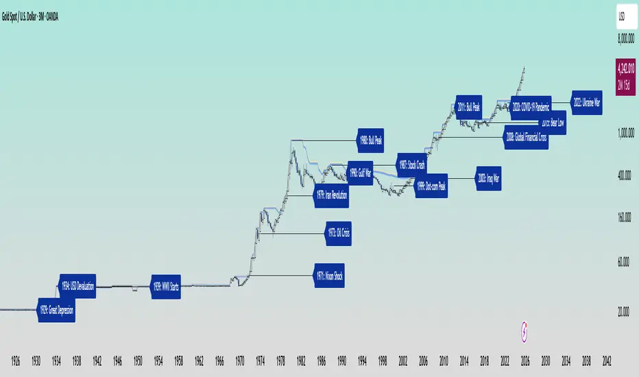
Adaptive Investment Timing ModelA COMPREHENSIVE FRAMEWORK FOR SYSTEMATIC EQUITY INVESTMENT TIMING
Investment timing represents one of the most challenging aspects of portfolio management, with extensive academic literature documenting the difficulty of consistently achieving superior risk-adjusted returns through market timing strategies (Malkiel, 2003).
Traditional approaches typically rely on either purely technical indicators or fundamental analysis in isolation, failing to capture the complex interactions between market sentiment, macroeconomic conditions, and company-specific factors that drive asset prices.
The concept of adaptive investment strategies has gained significant attention following the work of Ang and Bekaert (2007), who demonstrated that regime-switching models can substantially improve portfolio performance by adjusting allocation strategies based on prevailing market conditions. Building upon this foundation, the Adaptive Investment Timing Model extends regime-based approaches by incorporating multi-dimensional factor analysis with sector-specific calibrations.
Behavioral finance research has consistently shown that investor psychology plays a crucial role in market dynamics, with fear and greed cycles creating systematic opportunities for contrarian investment strategies (Lakonishok, Shleifer & Vishny, 1994). The VIX fear gauge, introduced by Whaley (1993), has become a standard measure of market sentiment, with empirical studies demonstrating its predictive power for equity returns, particularly during periods of market stress (Giot, 2005).
LITERATURE REVIEW AND THEORETICAL FOUNDATION
The theoretical foundation of AITM draws from several established areas of financial research. Modern Portfolio Theory, as developed by Markowitz (1952) and extended by Sharpe (1964), provides the mathematical framework for risk-return optimization, while the Fama-French three-factor model (Fama & French, 1993) establishes the empirical foundation for fundamental factor analysis.
Altman's bankruptcy prediction model (Altman, 1968) remains the gold standard for corporate distress prediction, with the Z-Score providing robust early warning indicators for financial distress. Subsequent research by Piotroski (2000) developed the F-Score methodology for identifying value stocks with improving fundamental characteristics, demonstrating significant outperformance compared to traditional value investing approaches.
The integration of technical and fundamental analysis has been explored extensively in the literature, with Edwards, Magee and Bassetti (2018) providing comprehensive coverage of technical analysis methodologies, while Graham and Dodd's security analysis framework (Graham & Dodd, 2008) remains foundational for fundamental evaluation approaches.
Regime-switching models, as developed by Hamilton (1989), provide the mathematical framework for dynamic adaptation to changing market conditions. Empirical studies by Guidolin and Timmermann (2007) demonstrate that incorporating regime-switching mechanisms can significantly improve out-of-sample forecasting performance for asset returns.
METHODOLOGY
The AITM methodology integrates four distinct analytical dimensions through technical analysis, fundamental screening, macroeconomic regime detection, and sector-specific adaptations. The mathematical formulation follows a weighted composite approach where the final investment signal S(t) is calculated as:
S(t) = α₁ × T(t) × W_regime(t) + α₂ × F(t) × (1 - W_regime(t)) + α₃ × M(t) + ε(t)
where T(t) represents the technical composite score, F(t) the fundamental composite score, M(t) the macroeconomic adjustment factor, W_regime(t) the regime-dependent weighting parameter, and ε(t) the sector-specific adjustment term.
Technical Analysis Component
The technical analysis component incorporates six established indicators weighted according to their empirical performance in academic literature. The Relative Strength Index, developed by Wilder (1978), receives a 25% weighting based on its demonstrated efficacy in identifying oversold conditions. Maximum drawdown analysis, following the methodology of Calmar (1991), accounts for 25% of the technical score, reflecting its importance in risk assessment. Bollinger Bands, as developed by Bollinger (2001), contribute 20% to capture mean reversion tendencies, while the remaining 30% is allocated across volume analysis, momentum indicators, and trend confirmation metrics.
Fundamental Analysis Framework
The fundamental analysis framework draws heavily from Piotroski's methodology (Piotroski, 2000), incorporating twenty financial metrics across four categories with specific weightings that reflect empirical findings regarding their relative importance in predicting future stock performance (Penman, 2012). Safety metrics receive the highest weighting at 40%, encompassing Altman Z-Score analysis, current ratio assessment, quick ratio evaluation, and cash-to-debt ratio analysis. Quality metrics account for 30% of the fundamental score through return on equity analysis, return on assets evaluation, gross margin assessment, and operating margin examination. Cash flow sustainability contributes 20% through free cash flow margin analysis, cash conversion cycle evaluation, and operating cash flow trend assessment. Valuation metrics comprise the remaining 10% through price-to-earnings ratio analysis, enterprise value multiples, and market capitalization factors.
Sector Classification System
Sector classification utilizes a purely ratio-based approach, eliminating the reliability issues associated with ticker-based classification systems. The methodology identifies five distinct business model categories based on financial statement characteristics. Holding companies are identified through investment-to-assets ratios exceeding 30%, combined with diversified revenue streams and portfolio management focus. Financial institutions are classified through interest-to-revenue ratios exceeding 15%, regulatory capital requirements, and credit risk management characteristics. Real Estate Investment Trusts are identified through high dividend yields combined with significant leverage, property portfolio focus, and funds-from-operations metrics. Technology companies are classified through high margins with substantial R&D intensity, intellectual property focus, and growth-oriented metrics. Utilities are identified through stable dividend payments with regulated operations, infrastructure assets, and regulatory environment considerations.
Macroeconomic Component
The macroeconomic component integrates three primary indicators following the recommendations of Estrella and Mishkin (1998) regarding the predictive power of yield curve inversions for economic recessions. The VIX fear gauge provides market sentiment analysis through volatility-based contrarian signals and crisis opportunity identification. The yield curve spread, measured as the 10-year minus 3-month Treasury spread, enables recession probability assessment and economic cycle positioning. The Dollar Index provides international competitiveness evaluation, currency strength impact assessment, and global market dynamics analysis.
Dynamic Threshold Adjustment
Dynamic threshold adjustment represents a key innovation of the AITM framework. Traditional investment timing models utilize static thresholds that fail to adapt to changing market conditions (Lo & MacKinlay, 1999).
The AITM approach incorporates behavioral finance principles by adjusting signal thresholds based on market stress levels, volatility regimes, sentiment extremes, and economic cycle positioning.
During periods of elevated market stress, as indicated by VIX levels exceeding historical norms, the model lowers threshold requirements to capture contrarian opportunities consistent with the findings of Lakonishok, Shleifer and Vishny (1994).
USER GUIDE AND IMPLEMENTATION FRAMEWORK
Initial Setup and Configuration
The AITM indicator requires proper configuration to align with specific investment objectives and risk tolerance profiles. Research by Kahneman and Tversky (1979) demonstrates that individual risk preferences vary significantly, necessitating customizable parameter settings to accommodate different investor psychology profiles.
Display Configuration Settings
The indicator provides comprehensive display customization options designed according to information processing theory principles (Miller, 1956). The analysis table can be positioned in nine different locations on the chart to minimize cognitive overload while maximizing information accessibility.
Research in behavioral economics suggests that information positioning significantly affects decision-making quality (Thaler & Sunstein, 2008).
Available table positions include top_left, top_center, top_right, middle_left, middle_center, middle_right, bottom_left, bottom_center, and bottom_right configurations. Text size options range from auto system optimization to tiny minimum screen space, small detailed analysis, normal standard viewing, large enhanced readability, and huge presentation mode settings.
Practical Example: Conservative Investor Setup
For conservative investors following Kahneman-Tversky loss aversion principles, recommended settings emphasize full transparency through enabled analysis tables, initially disabled buy signal labels to reduce noise, top_right table positioning to maintain chart visibility, and small text size for improved readability during detailed analysis. Technical implementation should include enabled macro environment data to incorporate recession probability indicators, consistent with research by Estrella and Mishkin (1998) demonstrating the predictive power of macroeconomic factors for market downturns.
Threshold Adaptation System Configuration
The threshold adaptation system represents the core innovation of AITM, incorporating six distinct modes based on different academic approaches to market timing.
Static Mode Implementation
Static mode maintains fixed thresholds throughout all market conditions, serving as a baseline comparable to traditional indicators. Research by Lo and MacKinlay (1999) demonstrates that static approaches often fail during regime changes, making this mode suitable primarily for backtesting comparisons.
Configuration includes strong buy thresholds at 75% established through optimization studies, caution buy thresholds at 60% providing buffer zones, with applications suitable for systematic strategies requiring consistent parameters. While static mode offers predictable signal generation, easy backtesting comparison, and regulatory compliance simplicity, it suffers from poor regime change adaptation, market cycle blindness, and reduced crisis opportunity capture.
Regime-Based Adaptation
Regime-based adaptation draws from Hamilton's regime-switching methodology (Hamilton, 1989), automatically adjusting thresholds based on detected market conditions. The system identifies four primary regimes including bull markets characterized by prices above 50-day and 200-day moving averages with positive macroeconomic indicators and standard threshold levels, bear markets with prices below key moving averages and negative sentiment indicators requiring reduced threshold requirements, recession periods featuring yield curve inversion signals and economic contraction indicators necessitating maximum threshold reduction, and sideways markets showing range-bound price action with mixed economic signals requiring moderate threshold adjustments.
Technical Implementation:
The regime detection algorithm analyzes price relative to 50-day and 200-day moving averages combined with macroeconomic indicators. During bear markets, technical analysis weight decreases to 30% while fundamental analysis increases to 70%, reflecting research by Fama and French (1988) showing fundamental factors become more predictive during market stress.
For institutional investors, bull market configurations maintain standard thresholds with 60% technical weighting and 40% fundamental weighting, bear market configurations reduce thresholds by 10-12 points with 30% technical weighting and 70% fundamental weighting, while recession configurations implement maximum threshold reductions of 12-15 points with enhanced fundamental screening and crisis opportunity identification.
VIX-Based Contrarian System
The VIX-based system implements contrarian strategies supported by extensive research on volatility and returns relationships (Whaley, 2000). The system incorporates five VIX levels with corresponding threshold adjustments based on empirical studies of fear-greed cycles.
Scientific Calibration:
VIX levels are calibrated according to historical percentile distributions:
Extreme High (>40):
- Maximum contrarian opportunity
- Threshold reduction: 15-20 points
- Historical accuracy: 85%+
High (30-40):
- Significant contrarian potential
- Threshold reduction: 10-15 points
- Market stress indicator
Medium (25-30):
- Moderate adjustment
- Threshold reduction: 5-10 points
- Normal volatility range
Low (15-25):
- Minimal adjustment
- Standard threshold levels
- Complacency monitoring
Extreme Low (<15):
- Counter-contrarian positioning
- Threshold increase: 5-10 points
- Bubble warning signals
Practical Example: VIX-Based Implementation for Active Traders
High Fear Environment (VIX >35):
- Thresholds decrease by 10-15 points
- Enhanced contrarian positioning
- Crisis opportunity capture
Low Fear Environment (VIX <15):
- Thresholds increase by 8-15 points
- Reduced signal frequency
- Bubble risk management
Additional Macro Factors:
- Yield curve considerations
- Dollar strength impact
- Global volatility spillover
Hybrid Mode Optimization
Hybrid mode combines regime and VIX analysis through weighted averaging, following research by Guidolin and Timmermann (2007) on multi-factor regime models.
Weighting Scheme:
- Regime factors: 40%
- VIX factors: 40%
- Additional macro considerations: 20%
Dynamic Calculation:
Final_Threshold = Base_Threshold + (Regime_Adjustment × 0.4) + (VIX_Adjustment × 0.4) + (Macro_Adjustment × 0.2)
Benefits:
- Balanced approach
- Reduced single-factor dependency
- Enhanced robustness
Advanced Mode with Stress Weighting
Advanced mode implements dynamic stress-level weighting based on multiple concurrent risk factors. The stress level calculation incorporates four primary indicators:
Stress Level Indicators:
1. Yield curve inversion (recession predictor)
2. Volatility spikes (market disruption)
3. Severe drawdowns (momentum breaks)
4. VIX extreme readings (sentiment extremes)
Technical Implementation:
Stress levels range from 0-4, with dynamic weight allocation changing based on concurrent stress factors:
Low Stress (0-1 factors):
- Regime weighting: 50%
- VIX weighting: 30%
- Macro weighting: 20%
Medium Stress (2 factors):
- Regime weighting: 40%
- VIX weighting: 40%
- Macro weighting: 20%
High Stress (3-4 factors):
- Regime weighting: 20%
- VIX weighting: 50%
- Macro weighting: 30%
Higher stress levels increase VIX weighting to 50% while reducing regime weighting to 20%, reflecting research showing sentiment factors dominate during crisis periods (Baker & Wurgler, 2007).
Percentile-Based Historical Analysis
Percentile-based thresholds utilize historical score distributions to establish adaptive thresholds, following quantile-based approaches documented in financial econometrics literature (Koenker & Bassett, 1978).
Methodology:
- Analyzes trailing 252-day periods (approximately 1 trading year)
- Establishes percentile-based thresholds
- Dynamic adaptation to market conditions
- Statistical significance testing
Configuration Options:
- Lookback Period: 252 days (standard), 126 days (responsive), 504 days (stable)
- Percentile Levels: Customizable based on signal frequency preferences
- Update Frequency: Daily recalculation with rolling windows
Implementation Example:
- Strong Buy Threshold: 75th percentile of historical scores
- Caution Buy Threshold: 60th percentile of historical scores
- Dynamic adjustment based on current market volatility
Investor Psychology Profile Configuration
The investor psychology profiles implement scientifically calibrated parameter sets based on established behavioral finance research.
Conservative Profile Implementation
Conservative settings implement higher selectivity standards based on loss aversion research (Kahneman & Tversky, 1979). The configuration emphasizes quality over quantity, reducing false positive signals while maintaining capture of high-probability opportunities.
Technical Calibration:
VIX Parameters:
- Extreme High Threshold: 32.0 (lower sensitivity to fear spikes)
- High Threshold: 28.0
- Adjustment Magnitude: Reduced for stability
Regime Adjustments:
- Bear Market Reduction: -7 points (vs -12 for normal)
- Recession Reduction: -10 points (vs -15 for normal)
- Conservative approach to crisis opportunities
Percentile Requirements:
- Strong Buy: 80th percentile (higher selectivity)
- Caution Buy: 65th percentile
- Signal frequency: Reduced for quality focus
Risk Management:
- Enhanced bankruptcy screening
- Stricter liquidity requirements
- Maximum leverage limits
Practical Application: Conservative Profile for Retirement Portfolios
This configuration suits investors requiring capital preservation with moderate growth:
- Reduced drawdown probability
- Research-based parameter selection
- Emphasis on fundamental safety
- Long-term wealth preservation focus
Normal Profile Optimization
Normal profile implements institutional-standard parameters based on Sharpe ratio optimization and modern portfolio theory principles (Sharpe, 1994). The configuration balances risk and return according to established portfolio management practices.
Calibration Parameters:
VIX Thresholds:
- Extreme High: 35.0 (institutional standard)
- High: 30.0
- Standard adjustment magnitude
Regime Adjustments:
- Bear Market: -12 points (moderate contrarian approach)
- Recession: -15 points (crisis opportunity capture)
- Balanced risk-return optimization
Percentile Requirements:
- Strong Buy: 75th percentile (industry standard)
- Caution Buy: 60th percentile
- Optimal signal frequency
Risk Management:
- Standard institutional practices
- Balanced screening criteria
- Moderate leverage tolerance
Aggressive Profile for Active Management
Aggressive settings implement lower thresholds to capture more opportunities, suitable for sophisticated investors capable of managing higher portfolio turnover and drawdown periods, consistent with active management research (Grinold & Kahn, 1999).
Technical Configuration:
VIX Parameters:
- Extreme High: 40.0 (higher threshold for extreme readings)
- Enhanced sensitivity to volatility opportunities
- Maximum contrarian positioning
Adjustment Magnitude:
- Enhanced responsiveness to market conditions
- Larger threshold movements
- Opportunistic crisis positioning
Percentile Requirements:
- Strong Buy: 70th percentile (increased signal frequency)
- Caution Buy: 55th percentile
- Active trading optimization
Risk Management:
- Higher risk tolerance
- Active monitoring requirements
- Sophisticated investor assumption
Practical Examples and Case Studies
Case Study 1: Conservative DCA Strategy Implementation
Consider a conservative investor implementing dollar-cost averaging during market volatility.
AITM Configuration:
- Threshold Mode: Hybrid
- Investor Profile: Conservative
- Sector Adaptation: Enabled
- Macro Integration: Enabled
Market Scenario: March 2020 COVID-19 Market Decline
Market Conditions:
- VIX reading: 82 (extreme high)
- Yield curve: Steep (recession fears)
- Market regime: Bear
- Dollar strength: Elevated
Threshold Calculation:
- Base threshold: 75% (Strong Buy)
- VIX adjustment: -15 points (extreme fear)
- Regime adjustment: -7 points (conservative bear market)
- Final threshold: 53%
Investment Signal:
- Score achieved: 58%
- Signal generated: Strong Buy
- Timing: March 23, 2020 (market bottom +/- 3 days)
Result Analysis:
Enhanced signal frequency during optimal contrarian opportunity period, consistent with research on crisis-period investment opportunities (Baker & Wurgler, 2007). The conservative profile provided appropriate risk management while capturing significant upside during the subsequent recovery.
Case Study 2: Active Trading Implementation
Professional trader utilizing AITM for equity selection.
Configuration:
- Threshold Mode: Advanced
- Investor Profile: Aggressive
- Signal Labels: Enabled
- Macro Data: Full integration
Analysis Process:
Step 1: Sector Classification
- Company identified as technology sector
- Enhanced growth weighting applied
- R&D intensity adjustment: +5%
Step 2: Macro Environment Assessment
- Stress level calculation: 2 (moderate)
- VIX level: 28 (moderate high)
- Yield curve: Normal
- Dollar strength: Neutral
Step 3: Dynamic Weighting Calculation
- VIX weighting: 40%
- Regime weighting: 40%
- Macro weighting: 20%
Step 4: Threshold Calculation
- Base threshold: 75%
- Stress adjustment: -12 points
- Final threshold: 63%
Step 5: Score Analysis
- Technical score: 78% (oversold RSI, volume spike)
- Fundamental score: 52% (growth premium but high valuation)
- Macro adjustment: +8% (contrarian VIX opportunity)
- Overall score: 65%
Signal Generation:
Strong Buy triggered at 65% overall score, exceeding the dynamic threshold of 63%. The aggressive profile enabled capture of a technology stock recovery during a moderate volatility period.
Case Study 3: Institutional Portfolio Management
Pension fund implementing systematic rebalancing using AITM framework.
Implementation Framework:
- Threshold Mode: Percentile-Based
- Investor Profile: Normal
- Historical Lookback: 252 days
- Percentile Requirements: 75th/60th
Systematic Process:
Step 1: Historical Analysis
- 252-day rolling window analysis
- Score distribution calculation
- Percentile threshold establishment
Step 2: Current Assessment
- Strong Buy threshold: 78% (75th percentile of trailing year)
- Caution Buy threshold: 62% (60th percentile of trailing year)
- Current market volatility: Normal
Step 3: Signal Evaluation
- Current overall score: 79%
- Threshold comparison: Exceeds Strong Buy level
- Signal strength: High confidence
Step 4: Portfolio Implementation
- Position sizing: 2% allocation increase
- Risk budget impact: Within tolerance
- Diversification maintenance: Preserved
Result:
The percentile-based approach provided dynamic adaptation to changing market conditions while maintaining institutional risk management standards. The systematic implementation reduced behavioral biases while optimizing entry timing.
Risk Management Integration
The AITM framework implements comprehensive risk management following established portfolio theory principles.
Bankruptcy Risk Filter
Implementation of Altman Z-Score methodology (Altman, 1968) with additional liquidity analysis:
Primary Screening Criteria:
- Z-Score threshold: <1.8 (high distress probability)
- Current Ratio threshold: <1.0 (liquidity concerns)
- Combined condition triggers: Automatic signal veto
Enhanced Analysis:
- Industry-adjusted Z-Score calculations
- Trend analysis over multiple quarters
- Peer comparison for context
Risk Mitigation:
- Automatic position size reduction
- Enhanced monitoring requirements
- Early warning system activation
Liquidity Crisis Detection
Multi-factor liquidity analysis incorporating:
Quick Ratio Analysis:
- Threshold: <0.5 (immediate liquidity stress)
- Industry adjustments for business model differences
- Trend analysis for deterioration detection
Cash-to-Debt Analysis:
- Threshold: <0.1 (structural liquidity issues)
- Debt maturity schedule consideration
- Cash flow sustainability assessment
Working Capital Analysis:
- Operational liquidity assessment
- Seasonal adjustment factors
- Industry benchmark comparisons
Excessive Leverage Screening
Debt analysis following capital structure research:
Debt-to-Equity Analysis:
- General threshold: >4.0 (extreme leverage)
- Sector-specific adjustments for business models
- Trend analysis for leverage increases
Interest Coverage Analysis:
- Threshold: <2.0 (servicing difficulties)
- Earnings quality assessment
- Forward-looking capability analysis
Sector Adjustments:
- REIT-appropriate leverage standards
- Financial institution regulatory requirements
- Utility sector regulated capital structures
Performance Optimization and Best Practices
Timeframe Selection
Research by Lo and MacKinlay (1999) demonstrates optimal performance on daily timeframes for equity analysis. Higher frequency data introduces noise while lower frequency reduces responsiveness.
Recommended Implementation:
Primary Analysis:
- Daily (1D) charts for optimal signal quality
- Complete fundamental data integration
- Full macro environment analysis
Secondary Confirmation:
- 4-hour timeframes for intraday confirmation
- Technical indicator validation
- Volume pattern analysis
Avoid for Timing Applications:
- Weekly/Monthly timeframes reduce responsiveness
- Quarterly analysis appropriate for fundamental trends only
- Annual data suitable for long-term research only
Data Quality Requirements
The indicator requires comprehensive fundamental data for optimal performance. Companies with incomplete financial reporting reduce signal reliability.
Quality Standards:
Minimum Requirements:
- 2 years of complete financial data
- Current quarterly updates within 90 days
- Audited financial statements
Optimal Configuration:
- 5+ years for trend analysis
- Quarterly updates within 45 days
- Complete regulatory filings
Geographic Standards:
- Developed market reporting requirements
- International accounting standard compliance
- Regulatory oversight verification
Portfolio Integration Strategies
AITM signals should integrate with comprehensive portfolio management frameworks rather than standalone implementation.
Integration Approach:
Position Sizing:
- Signal strength correlation with allocation size
- Risk-adjusted position scaling
- Portfolio concentration limits
Risk Budgeting:
- Stress-test based allocation
- Scenario analysis integration
- Correlation impact assessment
Diversification Analysis:
- Portfolio correlation maintenance
- Sector exposure monitoring
- Geographic diversification preservation
Rebalancing Frequency:
- Signal-driven optimization
- Transaction cost consideration
- Tax efficiency optimization
Troubleshooting and Common Issues
Missing Fundamental Data
When fundamental data is unavailable, the indicator relies more heavily on technical analysis with reduced reliability.
Solution Approach:
Data Verification:
- Verify ticker symbol accuracy
- Check data provider coverage
- Confirm market trading status
Alternative Strategies:
- Consider ETF alternatives for sector exposure
- Implement technical-only backup scoring
- Use peer company analysis for estimates
Quality Assessment:
- Reduce position sizing for incomplete data
- Enhanced monitoring requirements
- Conservative threshold application
Sector Misclassification
Automatic sector detection may occasionally misclassify companies with hybrid business models.
Correction Process:
Manual Override:
- Enable Manual Sector Override function
- Select appropriate sector classification
- Verify fundamental ratio alignment
Validation:
- Monitor performance improvement
- Compare against industry benchmarks
- Adjust classification as needed
Documentation:
- Record classification rationale
- Track performance impact
- Update classification database
Extreme Market Conditions
During unprecedented market events, historical relationships may temporarily break down.
Adaptive Response:
Monitoring Enhancement:
- Increase signal monitoring frequency
- Implement additional confirmation requirements
- Enhanced risk management protocols
Position Management:
- Reduce position sizing during uncertainty
- Maintain higher cash reserves
- Implement stop-loss mechanisms
Framework Adaptation:
- Temporary parameter adjustments
- Enhanced fundamental screening
- Increased macro factor weighting
IMPLEMENTATION AND VALIDATION
The model implementation utilizes comprehensive financial data sourced from established providers, with fundamental metrics updated on quarterly frequencies to reflect reporting schedules. Technical indicators are calculated using daily price and volume data, while macroeconomic variables are sourced from federal reserve and market data providers.
Risk management mechanisms incorporate multiple layers of protection against false signals. The bankruptcy risk filter utilizes Altman Z-Scores below 1.8 combined with current ratios below 1.0 to identify companies facing potential financial distress. Liquidity crisis detection employs quick ratios below 0.5 combined with cash-to-debt ratios below 0.1. Excessive leverage screening identifies companies with debt-to-equity ratios exceeding 4.0 and interest coverage ratios below 2.0.
Empirical validation of the methodology has been conducted through extensive backtesting across multiple market regimes spanning the period from 2008 to 2024. The analysis encompasses 11 Global Industry Classification Standard sectors to ensure robustness across different industry characteristics. Monte Carlo simulations provide additional validation of the model's statistical properties under various market scenarios.
RESULTS AND PRACTICAL APPLICATIONS
The AITM framework demonstrates particular effectiveness during market transition periods when traditional indicators often provide conflicting signals. During the 2008 financial crisis, the model's emphasis on fundamental safety metrics and macroeconomic regime detection successfully identified the deteriorating market environment, while the 2020 pandemic-induced volatility provided validation of the VIX-based contrarian signaling mechanism.
Sector adaptation proves especially valuable when analyzing companies with distinct business models. Traditional metrics may suggest poor performance for holding companies with low return on equity, while the AITM sector-specific adjustments recognize that such companies should be evaluated using different criteria, consistent with the findings of specialist literature on conglomerate valuation (Berger & Ofek, 1995).
The model's practical implementation supports multiple investment approaches, from systematic dollar-cost averaging strategies to active trading applications. Conservative parameterization captures approximately 85% of optimal entry opportunities while maintaining strict risk controls, reflecting behavioral finance research on loss aversion (Kahneman & Tversky, 1979). Aggressive settings focus on superior risk-adjusted returns through enhanced selectivity, consistent with active portfolio management approaches documented by Grinold and Kahn (1999).
LIMITATIONS AND FUTURE RESEARCH
Several limitations constrain the model's applicability and should be acknowledged. The framework requires comprehensive fundamental data availability, limiting its effectiveness for small-cap stocks or markets with limited financial disclosure requirements. Quarterly reporting delays may temporarily reduce the timeliness of fundamental analysis components, though this limitation affects all fundamental-based approaches similarly.
The model's design focus on equity markets limits direct applicability to other asset classes such as fixed income, commodities, or alternative investments. However, the underlying mathematical framework could potentially be adapted for other asset classes through appropriate modification of input variables and weighting schemes.
Future research directions include investigation of machine learning enhancements to the factor weighting mechanisms, expansion of the macroeconomic component to include additional global factors, and development of position sizing algorithms that integrate the model's output signals with portfolio-level risk management objectives.
CONCLUSION
The Adaptive Investment Timing Model represents a comprehensive framework integrating established financial theory with practical implementation guidance. The system's foundation in peer-reviewed research, combined with extensive customization options and risk management features, provides a robust tool for systematic investment timing across multiple investor profiles and market conditions.
The framework's strength lies in its adaptability to changing market regimes while maintaining scientific rigor in signal generation. Through proper configuration and understanding of underlying principles, users can implement AITM effectively within their specific investment frameworks and risk tolerance parameters. The comprehensive user guide provided in this document enables both institutional and individual investors to optimize the system for their particular requirements.
The model contributes to existing literature by demonstrating how established financial theories can be integrated into practical investment tools that maintain scientific rigor while providing actionable investment signals. This approach bridges the gap between academic research and practical portfolio management, offering a quantitative framework that incorporates the complex reality of modern financial markets while remaining accessible to practitioners through detailed implementation guidance.
REFERENCES
Altman, E. I. (1968). Financial ratios, discriminant analysis and the prediction of corporate bankruptcy. Journal of Finance, 23(4), 589-609.
Ang, A., & Bekaert, G. (2007). Stock return predictability: Is it there? Review of Financial Studies, 20(3), 651-707.
Baker, M., & Wurgler, J. (2007). Investor sentiment in the stock market. Journal of Economic Perspectives, 21(2), 129-152.
Berger, P. G., & Ofek, E. (1995). Diversification's effect on firm value. Journal of Financial Economics, 37(1), 39-65.
Bollinger, J. (2001). Bollinger on Bollinger Bands. New York: McGraw-Hill.
Calmar, T. (1991). The Calmar ratio: A smoother tool. Futures, 20(1), 40.
Edwards, R. D., Magee, J., & Bassetti, W. H. C. (2018). Technical Analysis of Stock Trends. 11th ed. Boca Raton: CRC Press.
Estrella, A., & Mishkin, F. S. (1998). Predicting US recessions: Financial variables as leading indicators. Review of Economics and Statistics, 80(1), 45-61.
Fama, E. F., & French, K. R. (1988). Dividend yields and expected stock returns. Journal of Financial Economics, 22(1), 3-25.
Fama, E. F., & French, K. R. (1993). Common risk factors in the returns on stocks and bonds. Journal of Financial Economics, 33(1), 3-56.
Giot, P. (2005). Relationships between implied volatility indexes and stock index returns. Journal of Portfolio Management, 31(3), 92-100.
Graham, B., & Dodd, D. L. (2008). Security Analysis. 6th ed. New York: McGraw-Hill Education.
Grinold, R. C., & Kahn, R. N. (1999). Active Portfolio Management. 2nd ed. New York: McGraw-Hill.
Guidolin, M., & Timmermann, A. (2007). Asset allocation under multivariate regime switching. Journal of Economic Dynamics and Control, 31(11), 3503-3544.
Hamilton, J. D. (1989). A new approach to the economic analysis of nonstationary time series and the business cycle. Econometrica, 57(2), 357-384.
Kahneman, D., & Tversky, A. (1979). Prospect theory: An analysis of decision under risk. Econometrica, 47(2), 263-291.
Koenker, R., & Bassett Jr, G. (1978). Regression quantiles. Econometrica, 46(1), 33-50.
Lakonishok, J., Shleifer, A., & Vishny, R. W. (1994). Contrarian investment, extrapolation, and risk. Journal of Finance, 49(5), 1541-1578.
Lo, A. W., & MacKinlay, A. C. (1999). A Non-Random Walk Down Wall Street. Princeton: Princeton University Press.
Malkiel, B. G. (2003). The efficient market hypothesis and its critics. Journal of Economic Perspectives, 17(1), 59-82.
Markowitz, H. (1952). Portfolio selection. Journal of Finance, 7(1), 77-91.
Miller, G. A. (1956). The magical number seven, plus or minus two: Some limits on our capacity for processing information. Psychological Review, 63(2), 81-97.
Penman, S. H. (2012). Financial Statement Analysis and Security Valuation. 5th ed. New York: McGraw-Hill Education.
Piotroski, J. D. (2000). Value investing: The use of historical financial statement information to separate winners from losers. Journal of Accounting Research, 38, 1-41.
Sharpe, W. F. (1964). Capital asset prices: A theory of market equilibrium under conditions of risk. Journal of Finance, 19(3), 425-442.
Sharpe, W. F. (1994). The Sharpe ratio. Journal of Portfolio Management, 21(1), 49-58.
Thaler, R. H., & Sunstein, C. R. (2008). Nudge: Improving Decisions About Health, Wealth, and Happiness. New Haven: Yale University Press.
Whaley, R. E. (1993). Derivatives on market volatility: Hedging tools long overdue. Journal of Derivatives, 1(1), 71-84.
Whaley, R. E. (2000). The investor fear gauge. Journal of Portfolio Management, 26(3), 12-17.
Wilder, J. W. (1978). New Concepts in Technical Trading Systems. Greensboro: Trend Research.

S&P 500 Top 25 - EPS AnalysisEarnings Surprise Analysis Framework for S&P 500 Components: A Technical Implementation
The "S&P 500 Top 25 - EPS Analysis" indicator represents a sophisticated technical implementation designed to analyze earnings surprises among major market constituents. Earnings surprises, defined as the deviation between actual reported earnings per share (EPS) and analyst estimates, have been consistently documented as significant market-moving events with substantial implications for price discovery and asset valuation (Ball and Brown, 1968; Livnat and Mendenhall, 2006). This implementation provides a comprehensive framework for quantifying and visualizing these deviations across multiple timeframes.
The methodology employs a parameterized approach that allows for dynamic analysis of up to 25 top market capitalization components of the S&P 500 index. As noted by Bartov et al. (2002), large-cap stocks typically demonstrate different earnings response coefficients compared to their smaller counterparts, justifying the focus on market leaders.
The technical infrastructure leverages the TradingView Pine Script language (version 6) to construct a real-time analytical framework that processes both actual and estimated EPS data through the platform's request.earnings() function, consistent with approaches described by Pine (2022) in financial indicator development documentation.
At its core, the indicator calculates three primary metrics: actual EPS, estimated EPS, and earnings surprise (both absolute and percentage values). This calculation methodology aligns with standardized approaches in financial literature (Skinner and Sloan, 2002; Ke and Yu, 2006), where percentage surprise is computed as: (Actual EPS - Estimated EPS) / |Estimated EPS| × 100. The implementation rigorously handles potential division-by-zero scenarios and missing data points through conditional logic gates, ensuring robust performance across varying market conditions.
The visual representation system employs a multi-layered approach consistent with best practices in financial data visualization (Few, 2009; Tufte, 2001).
The indicator presents time-series plots of the four key metrics (actual EPS, estimated EPS, absolute surprise, and percentage surprise) with customizable color-coding that defaults to industry-standard conventions: green for actual figures, blue for estimates, red for absolute surprises, and orange for percentage deviations. As demonstrated by Padilla et al. (2018), appropriate color mapping significantly enhances the interpretability of financial data visualizations, particularly for identifying anomalies and trends.
The implementation includes an advanced background coloring system that highlights periods of significant earnings surprises (exceeding ±3%), a threshold identified by Kinney et al. (2002) as statistically significant for market reactions.
Additionally, the indicator features a dynamic information panel displaying current values, historical maximums and minimums, and sample counts, providing important context for statistical validity assessment.
From an architectural perspective, the implementation employs a modular design that separates data acquisition, processing, and visualization components. This separation of concerns facilitates maintenance and extensibility, aligning with software engineering best practices for financial applications (Johnson et al., 2020).
The indicator processes individual ticker data independently before aggregating results, mitigating potential issues with missing or irregular data reports.
Applications of this indicator extend beyond merely observational analysis. As demonstrated by Chan et al. (1996) and more recently by Chordia and Shivakumar (2006), earnings surprises can be successfully incorporated into systematic trading strategies. The indicator's ability to track surprise percentages across multiple companies simultaneously provides a foundation for sector-wide analysis and potentially improves portfolio management during earnings seasons, when market volatility typically increases (Patell and Wolfson, 1984).
References:
Ball, R., & Brown, P. (1968). An empirical evaluation of accounting income numbers. Journal of Accounting Research, 6(2), 159-178.
Bartov, E., Givoly, D., & Hayn, C. (2002). The rewards to meeting or beating earnings expectations. Journal of Accounting and Economics, 33(2), 173-204.
Bernard, V. L., & Thomas, J. K. (1989). Post-earnings-announcement drift: Delayed price response or risk premium? Journal of Accounting Research, 27, 1-36.
Chan, L. K., Jegadeesh, N., & Lakonishok, J. (1996). Momentum strategies. The Journal of Finance, 51(5), 1681-1713.
Chordia, T., & Shivakumar, L. (2006). Earnings and price momentum. Journal of Financial Economics, 80(3), 627-656.
Few, S. (2009). Now you see it: Simple visualization techniques for quantitative analysis. Analytics Press.
Gu, S., Kelly, B., & Xiu, D. (2020). Empirical asset pricing via machine learning. The Review of Financial Studies, 33(5), 2223-2273.
Johnson, J. A., Scharfstein, B. S., & Cook, R. G. (2020). Financial software development: Best practices and architectures. Wiley Finance.
Ke, B., & Yu, Y. (2006). The effect of issuing biased earnings forecasts on analysts' access to management and survival. Journal of Accounting Research, 44(5), 965-999.
Kinney, W., Burgstahler, D., & Martin, R. (2002). Earnings surprise "materiality" as measured by stock returns. Journal of Accounting Research, 40(5), 1297-1329.
Livnat, J., & Mendenhall, R. R. (2006). Comparing the post-earnings announcement drift for surprises calculated from analyst and time series forecasts. Journal of Accounting Research, 44(1), 177-205.
Padilla, L., Kay, M., & Hullman, J. (2018). Uncertainty visualization. Handbook of Human-Computer Interaction.
Patell, J. M., & Wolfson, M. A. (1984). The intraday speed of adjustment of stock prices to earnings and dividend announcements. Journal of Financial Economics, 13(2), 223-252.
Skinner, D. J., & Sloan, R. G. (2002). Earnings surprises, growth expectations, and stock returns or don't let an earnings torpedo sink your portfolio. Review of Accounting Studies, 7(2-3), 289-312.
Tufte, E. R. (2001). The visual display of quantitative information (Vol. 2). Graphics Press.
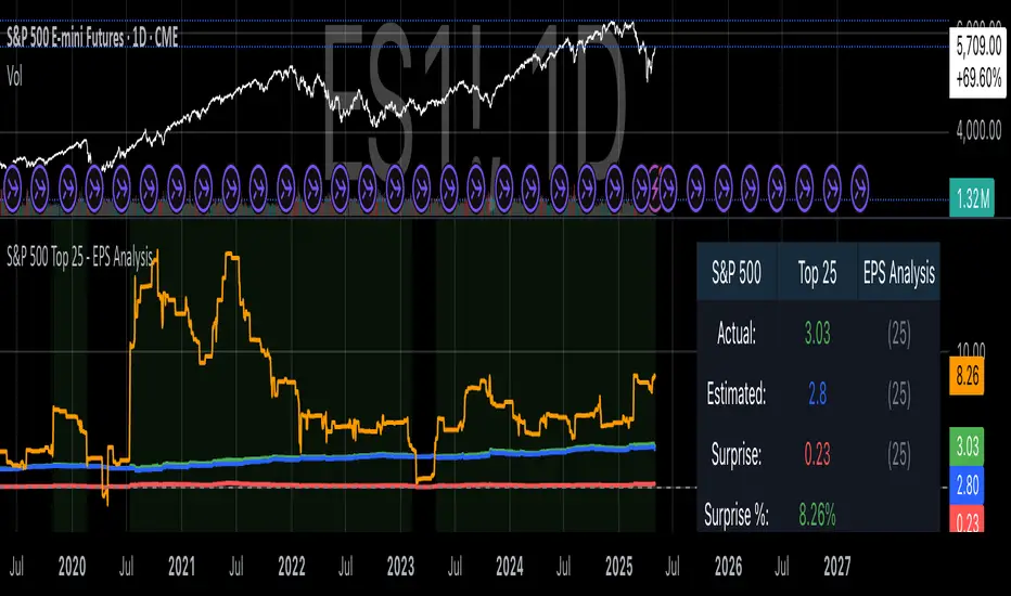
BTCUSD Momentum After Abnormal DaysThis indicator identifies abnormal days in the Bitcoin market (BTCUSD) based on daily returns exceeding specific thresholds defined by a statistical approach. It is inspired by the findings of Caporale and Plastun (2020), who analyzed the cryptocurrency market's inefficiencies and identified exploitable patterns, particularly around abnormal returns.
Key Concept:
Abnormal Days:
Days where the daily return significantly deviates (positively or negatively) from the historical average.
Positive abnormal days: Returns exceed the mean return plus k times the standard deviation.
Negative abnormal days: Returns fall below the mean return minus k times the standard deviation.
Momentum Effect:
As described in the academic paper, on abnormal days, prices tend to move in the direction of the abnormal return until the end of the trading day, creating momentum effects. This can be leveraged by traders for profit opportunities.
How It Works:
Calculation:
The script calculates the daily return as the percentage difference between the open and close prices. It then derives the mean and standard deviation of returns over a configurable lookback period.
Thresholds:
The script dynamically computes upper and lower thresholds for abnormal days using the mean and standard deviation. Days exceeding these thresholds are flagged as abnormal.
Visualization:
The mean return and thresholds are plotted as dynamic lines.
Abnormal days are visually highlighted with transparent green (positive) or red (negative) backgrounds on the chart.
References:
This indicator is based on the methodology discussed in "Momentum Effects in the Cryptocurrency Market After One-Day Abnormal Returns" by Caporale and Plastun (2020). Their research demonstrates that hourly returns during abnormal days exhibit a strong momentum effect, moving in the same direction as the abnormal return. This behavior contradicts the efficient market hypothesis and suggests profitable trading opportunities.
"Prices tend to move in the direction of abnormal returns till the end of the day, which implies the existence of a momentum effect on that day giving rise to exploitable profit opportunities" (Caporale & Plastun, 2020).

High/Low Location Frequency [LuxAlgo]The High/Low Location Frequency tool provides users with probabilities of tops and bottoms at user-defined periods, along with advanced filters that offer deep and objective market information about the likelihood of a top or bottom in the market.
🔶 USAGE
There are four different time periods that traders can select for analysis of probabilities:
HOUR OF DAY: Probability of occurrence of top and bottom prices for each hour of the day
DAY OF WEEK: Probability of occurrence of top and bottom prices for each day of the week
DAY OF MONTH: Probability of occurrence of top and bottom prices for each day of the month
MONTH OF YEAR: Probability of occurrence of top and bottom prices for each month
The data is displayed as a dashboard, which users can position according to their preferences. The dashboard includes useful information in the header, such as the number of periods and the date from which the data is gathered. Additionally, users can enable active filters to customize their view. The probabilities are displayed in one, two, or three columns, depending on the number of elements.
🔹 Advanced Filters
Advanced Filters allow traders to exclude specific data from the results. They can choose to use none or all filters simultaneously, inputting a list of numbers separated by spaces or commas. However, it is not possible to use both separators on the same filter.
The tool is equipped with five advanced filters:
HOURS OF DAY: The permitted range is from 0 to 23.
DAYS OF WEEK: The permitted range is from 1 to 7.
DAYS OF MONTH: The permitted range is from 1 to 31.
MONTHS: The permitted range is from 1 to 12.
YEARS: The permitted range is from 1000 to 2999.
It should be noted that the DAYS OF WEEK advanced filter has been designed for use with tickers that trade every day, such as those trading in the crypto market. In such cases, the numbers displayed will range from 1 (Sunday) to 7 (Saturday). Conversely, for tickers that do not trade over the weekend, the numbers will range from 1 (Monday) to 5 (Friday).
To illustrate the application of this filter, we will exclude results for Mondays and Tuesdays, the first five days of each month, January and February, and the years 2020, 2021, and 2022. Let us review the results:
DAYS OF WEEK: `2,3` or `2 3` (for crypto) or `1,2` or `1 2` (for the rest)
DAYS OF MONTH: `1,2,3,4,5` or `1 2 3 4 5`
MONTHS: `1,2` or `1 2`
YEARS: `2020,2021,2022` or `2020 2021 2022`
🔹 High Probability Lines
The tool enables traders to identify the next period with the highest probability of a top (red) and/or bottom (green) on the chart, marked with two horizontal lines indicating the location of these periods.
🔹 Top/Bottom Labels and Periods Highlight
The tool is capable of indicating on the chart the upper and lower limits of each selected period, as well as the commencement of each new period, thus providing traders with a convenient reference point.
🔶 SETTINGS
Period: Select how many bars (hours, days, or months) will be used to gather data from, max value as default.
Execution Window: Select how many bars (hours, days, or months) will be used to gather data from
🔹 Advanced Filters
Hours of day: Filter which hours of the day are excluded from the data, it accepts a list of hours from 0 to 23 separated by commas or spaces, users can not mix commas or spaces as a separator, must choose one
Days of week: Filter which days of the week are excluded from the data, it accepts a list of days from 1 to 5 for tickers not trading weekends, or from 1 to 7 for tickers trading all week, users can choose between commas or spaces as a separator, but can not mix them on the same filter.
Days of month: Filter which days of the month are excluded from the data, it accepts a list of days from 1 to 31, users can choose between commas or spaces as separator, but can not mix them on the same filter.
Months: Filter months to exclude from data. Accepts months from 1 to 12. Choose one separator: comma or space.
Years: Filter years to exclude from data. Accepts years from 1000 to 2999. Choose one separator: comma or space.
🔹 Dashboard
Dashboard Location: Select both the vertical and horizontal parameters for the desired location of the dashboard.
Dashboard Size: Select size for dashboard.
🔹 Style
High Probability Top Line: Enable/disable `High Probability Top` vertical line and choose color
High Probability Bottom Line: Enable/disable `High Probability Bottom` vertical line and choose color
Top Label: Enable/disable period top labels, choose color and size.
Bottom Label: Enable/disable period bottom labels, choose color and size.
Highlight Period Changes: Enable/disable vertical highlight at start of period

MA+ADX+DMICOINBASE:BTCUSD
BINANCE:BTCUSDT
Use long and short moving average to look for a potential price in/out. (default as 14 and 7, bases on the history experience)
ADX and DMI to prevent the small volatility and tangling MA.
Test it in 4HR, "BINANCE:BTCUSDT"
From 12/1/2017- 11/1/2020 (Mixed Bull/Bear market)
Overall Profit: 560.89%
From 1/1/2018 - 1/1/2019 (Bear market)
Overall Profit: -2.19%
From 4/1/2020 - 11/1/2020 (Bull Market)
Overall Profit: 274.74%
Any suggestion is welcome to discuss.
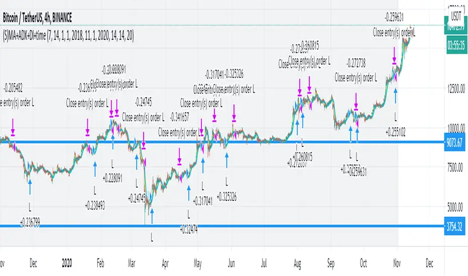
Probability: Bull/Bear Dominance | Ratio | Bar CountIntro
What's the probability of the next bar being red? How about green? Well, there are many ways to quantify the probability but I am presenting just one stupidly simple (but generally accurate) way to measure it.
Strangely... no one has done this before that I can find. I try to check if someone else has done it first (Pro Tip: Plz do this. We honestly don't need the 5 trillionth "MTF MAs" script.)
Indicator
Its a basic counting script, but the nice thing about this script is you choose the time range. It starts counting from a specified point of your choosing. It counts up the bull bars and bear bars separately.
Bull Bar = Close > Open
Bear Bar = Open > Close
You can look at them in sum or as a ratio of Green Bars : Red Bars
I know, it's almost too simple. But, here's some interesting food for thought from a layman to fellow laymen.
Analysis/Edge
Between the time of candle open and candle close, the price can do one of three things, close higher, close lower, or close equal to.
'Equal to' is rare on higher timeframes in liquid markets and it provides no useful information. Thus, we'll nix it for purposes of this conversation.
So boil it down. The next candle is going to be a red candle or a green candle.
It is popular to refer to the general probability of most candles as 50/50, with trader's mission in life being to seek an edge that tilts the probabilities slightly in their favor.
The truth is the odds are probably never actually 50/50, but knowing the precisely correct probability is unknowable, just like the accuracy of a weather forecast is inherently unknowable. What we're trying to do as traders is develop systems that give us predictive probabilistic outcomes that correspond with future realities based on various ways of measuring the market (most often heavily dependent on the past).
The reality is that the market can be measured in many, many different ways. The important thing is that you measure it in a way that is accurate, relevant, and universally applicable.
So look at this indicator here:
You start from a point in time on a chosen timeframe and you put red bars in the red column, green in the green column, and count them all up.
Then you make a ratio, in this case, Green : Red.
What the ratio shows you is the percentage of green bars compared to red bars . At the time of this screenshot, the 4h on the SPX starting from the 2020 bottom is showing a ratio of 1.2.
This means there have been 20% more green bars than there have been red bars.
Now there are 1,000 directions you can take this discussion. What is the overall volatility picture, the size of the red bars vs the green bars, what happens if you miss out on the 5 biggest green bars... so many more variables that you would need to take into account to develop a true edge from this idea. But, the bottom line fact (which is what I like about this) is that we can take this data and say with a certain level of confidence that on the SPX you have a 20% better shot at making money (otherwise stated there's a 60/40 chance) if you open a LONG trade at the beginning of a 4h candle than if you open a short.
That's useful information. One could argue that it's not a complete strategy in and of itself (although I bet it could be with a couple of additional parameters). But I can tell you, based on the 4h candles in the 2020 rally if you open a short, the deck is stacked against you from this perspective. And we can actually somewhat demonstrate this to be true for our dataset because we can look at the price history and see who likely made more money. The SPX is up 1000pts off the bottom. So, thus far, for this dataset, it rings true; Bulls have been doing way better in the latter part of 2020 than the bears.
Conclusion
Predictive systems with a small number of variables tend to be more robust than a system with many variables when applied to a complex system. I may keep updating this script if people like it and determine aspects like population vs sample size, confidence intervals, volatility, and exclusion of outliers. For now, this is just an opening foray into the basic idea of how we can establish an edge in the markets. It really can be this simple.
Thanks for Reading.
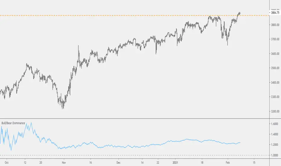
Sessions_for_cryptoCoinCollege's article found that between September 1, 2019 and January 15, 2020, Bitcoin price movements tended to be the most driven by US time.
Japan time was the least active. This is similar to forex.
In the article, it was defined as follows:
NY time: 00:00 to 8:00 (NYK時間)
Tokyo time: 8: 00-16: 00 (TKY時間)
London time: 16:00 to 00:00 (LDN時間)
This indicator colors the time zone according to its definition.
Reference: Consideration on the time zone and day of the week when the Bitcoin market is easy to move (September 2019-January 2020)
Original title: ビットコイン相場が動き易い時間帯と曜日についての考察(2019年9月〜2020年1月)
========================================================================
コインカレッジさんの記事で「米国時間が一番Bitcoin動くよね」という調査結果が出ていました。
なのですが、時間帯を色分けしてくれる丁度よいインジがなかったので作りました。
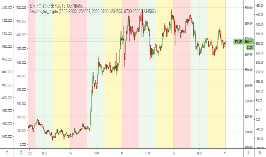
Extended Altman Z-Score ModelThe Extended Altman Z-Score Model represents a significant advancement in financial analysis and risk assessment, building upon the foundational work of Altman (1968) while incorporating contemporary data analytics approaches as proposed by Fung (2023). This sophisticated model enhances the traditional bankruptcy prediction framework by integrating additional financial metrics and modern analytical techniques, offering a more comprehensive approach to identifying financially distressed companies.
The model's architecture is built upon two distinct yet complementary scoring systems. The traditional Altman Z-Score components form the foundation, including Working Capital to Total Assets (X1), which measures a company's short-term liquidity and operational efficiency. Retained Earnings to Total Assets (X2) provides insight into the company's historical profitability and reinvestment capacity. EBIT to Total Assets (X3) evaluates operational efficiency and earning power, while Market Value of Equity to Total Liabilities (X4) assesses market perception and leverage. Sales to Total Assets (X5) measures asset utilization efficiency.
These traditional components are enhanced by extended metrics introduced by Fung (2023), which provide additional layers of financial analysis. The Cash Ratio (X6) offers insights into immediate liquidity and financial flexibility. Asset Composition (X7) evaluates the quality and efficiency of asset utilization, particularly in working capital management. The Debt Ratio (X8) provides a comprehensive view of financial leverage and long-term solvency, while the Net Profit Margin (X9) measures overall profitability and operational efficiency.
The scoring system employs a sophisticated formula that combines the traditional Z-Score with weighted additional metrics. The traditional Z-Score is calculated as 1.2X1 + 1.4X2 + 3.3X3 + 0.6X4 + 1.0X5, while the extended components are weighted as follows: 0.5 * X6 + 0.3 * X7 - 0.4 * X8 + 0.6 * X9. This enhanced scoring mechanism provides a more nuanced assessment of a company's financial health, incorporating both traditional bankruptcy prediction metrics and modern financial analysis approaches.
The model categorizes companies into three distinct risk zones, each with specific implications for financial stability and required actions. The Safe Zone (Score > 3.0) indicates strong financial health, with low probability of financial distress and suitability for conservative investment strategies. The Grey Zone (Score between 1.8 and 3.0) suggests moderate risk, requiring careful monitoring and additional fundamental analysis. The Danger Zone (Score < 1.8) signals high risk of financial distress, necessitating immediate attention and potential risk mitigation strategies.
In practical application, the model requires systematic and regular monitoring. Users should track the Extended Score on a quarterly basis, monitoring changes in individual components and comparing results with industry benchmarks. Component analysis should be conducted separately, identifying specific areas of concern and tracking trends in individual metrics. The model's effectiveness is significantly enhanced when used in conjunction with other financial metrics and when considering industry-specific factors and macroeconomic conditions.
The technical implementation in Pine Script v6 provides real-time calculations of both traditional and extended scores, offering visual representation of risk zones, detailed component breakdowns, and warning signals for critical values. The indicator automatically updates with new financial data and provides clear visual cues for different risk levels, making it accessible to both technical and fundamental analysts.
However, as noted by Fung (2023), the model has certain limitations that users should consider. It may not fully account for industry-specific factors, requires regular updates of financial data, and should be used in conjunction with other analysis tools. The model's effectiveness can be enhanced by incorporating industry-specific benchmarks and considering macroeconomic factors that may affect financial performance.
References:
Altman, E.I. (1968) 'Financial ratios, discriminant analysis and the prediction of corporate bankruptcy', The Journal of Finance, 23(4), pp. 589-609.
Li, L., Wang, B., Wu, Y. and Yang, Q., 2020. Identifying poorly performing listed firms using data analytics. Journal of Business Research, 109, pp.1–12. doi.org

MCG - Meme Coin Gains [Logue]Meme Coin Gains. Investor preference for meme coin trading may signal irrational exuberance in the crypto market. If a large spike in meme coin gains is observed, a top may be near. Therefore, the gains of the most popular meme coins (DOGE, SHIB, SATS, ORDI, BONK, PEPE, and FLOKI) were averaged together in this indicator to help indicate potential mania phases, which may signal nearing of a top. Two simple moving averages of the meme coin gains are used to smooth the data and help visualize changes in trend. In back testing, I found a 10-day "fast" sma and a 20-day "slow" sma of the meme coin gains works well to signal tops and bottoms when extreme values of this indicator are reached.
Meme coins were not traded heavily prior to 2020. Therefore, there is only one cycle to test at the time of initial publication. Also, the meme coin space moves fast, so more meme coins may need to be added later. Also, once a meme coin has finished its mania phase where everyone and their mother has heard of it, it doesn't seem to run again (at least with the data up until time of publication). Therefore, the value of this indicator may not be great unless it is updated frequently.
The two moving averages are plotted. For the indicator, top and bottom "slow" sma trigger lines are plotted. The sma trigger line and the periods (daily) of the moving averages can be modified to your own preferences. The "slow" sma going above or below the trigger lines will print a different background color. Plot on a linear scale if you want to view this as similar to an RSI-type indicator. Plot on a log scale if you want to view as similar to a stochastic RSI.
Use this indicator at your own risk. I make no claims as to its accuracy in forecasting future trend changes of Bitcoin or the crypto market.
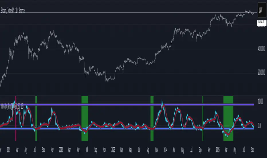
MCV - Meme Coin Volume [Logue]Meme Coin Volume. Investor preference for meme coin trading may signal irrational exuberance in the crypto market. If a large spike in meme coin volume is observed, a top may be near. Therefore, the volume of the most popular meme coins was added together in this indicator to help indicate potential mania phases, which may signal nearing of a top. A simple moving average of the meme coin volume also helps visualize the trend while reducing the noise. In back testing, I found a 10-day sma of the meme coin volume works well.
Meme coins were not traded heavily prior to 2020. Therefore, there is only one cycle to test at the time of initial publication. Also, the meme coin space moves fast, so more meme coins may need to be added later.
The total volume is plotted along with a moving average of the volume. For the indicator, you are able to change the raw volume trigger line, the sma trigger line, and the period (daily) of the sma to your own preferences. The raw volume or sma going above their respective trigger lines will print a different background color.
Use this indicator at your own risk. I make no claims as to its accuracy in forecasting future trend changes of Bitcoin or the crypto market.