Mean Reversion [SIMI]This mean reversion indicator identifies extreme price deviations from the mean, providing high-probability reversal signals. Designed for confluence-based trading, it works best when combined with complementary indicators such as VWAP, price action, and volume analysis.
📊 Core Features
Signal Types
Prime Signals (Bright Green/Red Dots): Extreme reversions usually beyond ±1.5 SD - highest probability setups (you can customise this zone!)
Regular Signals (Dark Green/Red Dots): Standard reversions - moderate probability
Leader Line (Pink Dotted): Early warning indicator for potential reversals
Histogram Weakness: Momentum divergence signals
Normalisation Methods:
Institutional Hybrid (Z-ATR) (Recommended): Volatility-adjusted Z-score - adapts to changing market conditions
Percentile Ranking: Statistical ranking - excellent for ranging markets
PPO + ATR Hybrid: Percentage-based with volatility adjustment
Efficiency Ratio: Trend-strength weighted
ATR: Pure volatility-based
None: Raw Z-score
⚙️ Quick Setup Guide
1. Institutional Presets
Pre-configured parameter sets optimised for different timeframes:
5M Day Trading (5/21/5): Intraday scalping
1H Options Trading (6/24/5): Options-focused setups
1D Monthly Cycle (5/20/5): Swing trading
2. Signal Filtering
Prime Thresholds: Adjust ±1.5 SD to control signal quality (tighter = fewer, higher quality, adjust this zone per asset traded)
Dot Filters: Fine-tune entry zones (-0.03/+0.03 default - this ignores noisy signals near Zero line)
Volume Filter: Enable to require volume confirmation (1.4x average recommended, but fine tune yourself)
3. Advanced Filters
Dynamic SD Thresholds: Auto-adjusts for volatility regimes (tighter in low vol, wider in high vol)
Time of Day Filter: Avoids first 30 minutes, last 15 minutes, and lunch hour (11:30-13:00 EST)
💡 Trading Strategy Recommendations
Optimal Usage
This indicator is not intended as a standalone system. Use it for confluence alongside:
VWAP (institutional positioning)
Price action (support/resistance)
Options flow (institutional direction)
Volume analysis (conviction confirmation)
Signal Interpretation
Prime Signals: Wait for these for highest-probability entries - mean reversion may take hours to days
Manual Entries: Don't wait for dots - trade the ±2 SD zones directly using your own confirmation
Options Strategy: Prime sell signals at +2 SD make excellent short call setups; prime buy signals at -2 SD for long calls
Timeframe Guidance
Lower Timeframes (1M-5M): Higher noise - require additional confluence
Higher Timeframes (1H-1D): More reliable signals - suitable for options and swing trades
Best Results: Multi-timeframe analysis (check 1H and 4H alignment on 5M entries)
🔔 Alert System
Master Alert
Enable customisable alerts via the Master Alert System:
Toggle individual signal types (Prime Buy/Sell, SD Crosses, Leader, Histogram)
Receives bespoke messages with ticker, timeframe, and price
One alert condition handles all selected signals
Individual Alerts
Separate alert conditions available for Prime and Regular signals if preferred.
📈 Backtesting Notes
Important: Backtest results are date-sensitive and should not be the primary focus. Instead:
Dial in settings visually on your chosen asset
Aim for signals near actual tops and bottoms
Test different normalisation methods for your specific instrument
Optimise for signal quality, not backtest ROI
Asset Testing: Primarily developed using SPY, QQQ, and IWM as main assets to trade. Other instruments may require parameter adjustment - mess around!
Backtest Engine
Entry/Exit modes (All Signals, Prime Only, Early Signals)
Position sizing (percentage-based)
Slippage and fill method (candle close recommended)
Date range selection
⚠️ Best Practices
Always use confluence - never trade on MR signals alone
Start with Institutional Hybrid normalisation - most adaptive to market conditions
Focus on Prime signals for quality over quantity
Test on your specific asset - optimal settings vary by instrument
Longer timeframes = higher reliability - 1H+ for best results
Enable Time Filter on intraday charts to avoid volatile periods
Use Dynamic SD in highly volatile markets (earnings, FOMC, etc.)
🛠️ Troubleshooting
Too many signals: Increase Prime Thresholds or enable Volume Filter
Too few signals: Decrease Prime Thresholds or reduce Dot Filters
False signals: Enable Time of Day Filter and Dynamic SD
Signals don't align with tops/bottoms: Try different normalisation method
📝 Feedback & Development
Bug Reports: Please report any issues via TradingView comments or direct message.
Strategy Sharing: I'd love to hear how you're using this indicator and what strategies you've developed.
Open Source: Feel free to fork and modify this indicator. If you create an improved version, please share it with the community!
🙏 Acknowledgements
Developed through AI-assisted collaboration.
Special thanks to Lazy Bear for his open source MACD histogram (volume based).
Open source forever - use freely, modify, and share.
Happy Trading!
Remember: Past performance does not guarantee future results. Always manage risk appropriately.
Pandas rock \m/
Mean_reversal

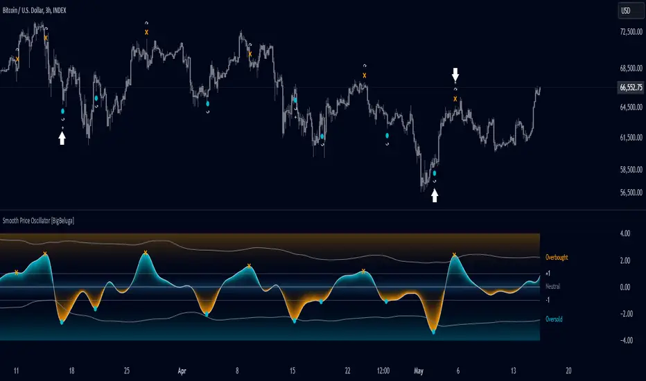
Smooth Price Oscillator [BigBeluga]The Smooth Price Oscillator by BigBeluga leverages John Ehlers' SuperSmoother filter to produce a clear and smooth oscillator for identifying market trends and mean reversion points. By filtering price data over two distinct periods, this indicator effectively removes noise, allowing traders to focus on significant signals without the clutter of market fluctuations.
🔵 KEY FEATURES & USAGE
● SuperSmoother-Based Oscillator:
This oscillator uses Ehlers' SuperSmoother filter, applied to two different periods, to create a smooth output that highlights price momentum and reduces market noise. The dual-period application enables a comparison of long-term and short-term price movements, making it suitable for both trend-following and reversion strategies.
// @function SuperSmoother filter based on Ehlers Filter
// @param price (float) The price series to be smoothed
// @param period (int) The smoothing period
// @returns Smoothed price
method smoother_F(float price, int period) =>
float step = 2.0 * math.pi / period
float a1 = math.exp(-math.sqrt(2) * math.pi / period)
float b1 = 2 * a1 * math.cos(math.sqrt(2) * step / period)
float c2 = b1
float c3 = -a1 * a1
float c1 = 1 - c2 - c3
float smoothed = 0.0
smoothed := bar_index >= 4
? c1 * (price + price ) / 2 + c2 * smoothed + c3 * smoothed
: price
smoothed
● Mean Reversion Signals:
The indicator identifies two types of mean reversion signals:
Simple Mean Reversion Signals: Triggered when the oscillator moves between thresholds of 1 and Overbought or between thresholds -1 and Ovesold, providing additional reversion opportunities. These signals are useful for capturing shorter-term corrections in trending markets.
Strong Mean Reversion Signals: Triggered when the oscillator above the overbought (upper band) or below oversold (lower band) thresholds, indicating a strong reversal point. These signals are marked with a "+" symbol on the chart for clear visibility.
Both types of signals are plotted on the oscillator and the main chart, helping traders to quickly identify potential trade entries or exits.
● Dynamic Bands and Thresholds:
The oscillator includes overbought and oversold bands based on a dynamically calculated standard deviation and EMA. These bands provide visual boundaries for identifying extreme price conditions, helping traders anticipate potential reversals at these levels.
● Real-Time Labels:
Labels are displayed at key thresholds and bands to indicate the oscillator’s status: "Overbought," "Oversold," and "Neutral". Mean reversion signals are also displayed on the main chart, providing an at-a-glance summary of current indicator conditions.
● Customizable Threshold Levels:
Traders can adjust the primary threshold and smoothing length according to their trading style. A higher threshold can reduce signal frequency, while a lower setting will provide more sensitivity to market reversals.
The Smooth Price Oscillator by BigBeluga is a refined, noise-filtered indicator designed to highlight mean reversion points with enhanced clarity. By providing both strong and simple reversion signals, as well as dynamic overbought/oversold bands, this tool allows traders to spot potential reversals and trend continuations with ease. Its dual representation on the oscillator and the main price chart offers flexibility and precision for any trading strategy focused on capturing cyclical market movements.
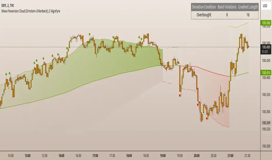
Mean Reversion Cloud (Ornstein-Uhlenbeck) // AlgoFyreThe Mean Reversion Cloud (Ornstein-Uhlenbeck) indicator detects mean-reversion opportunities by applying the Ornstein-Uhlenbeck process. It calculates a dynamic mean using an Exponential Weighted Moving Average, surrounded by volatility bands, signaling potential buy/sell points when prices deviate.
TABLE OF CONTENTS
🔶 ORIGINALITY
🔸Adaptive Mean Calculation
🔸Volatility-Based Cloud
🔸Speed of Reversion (θ)
🔶 FUNCTIONALITY
🔸Dynamic Mean and Volatility Bands
🞘 How it works
🞘 How to calculate
🞘 Code extract
🔸Visualization via Table and Plotshapes
🞘 Table Overview
🞘 Plotshapes Explanation
🞘 Code extract
🔶 INSTRUCTIONS
🔸Step-by-Step Guidelines
🞘 Setting Up the Indicator
🞘 Understanding What to Look For on the Chart
🞘 Possible Entry Signals
🞘 Possible Take Profit Strategies
🞘 Possible Stop-Loss Levels
🞘 Additional Tips
🔸Customize settings
🔶 CONCLUSION
▅▅▅▅▅▅▅▅▅▅▅▅▅▅▅▅▅▅▅▅▅▅▅▅▅▅▅▅▅▅▅▅▅▅▅▅▅▅▅▅▅▅▅▅▅▅
🔶 ORIGINALITY The Mean Reversion Cloud (Ornstein-Uhlenbeck) is a unique indicator that applies the Ornstein-Uhlenbeck stochastic process to identify mean-reverting behavior in asset prices. Unlike traditional moving average-based indicators, this model uses an Exponentially Weighted Moving Average (EWMA) to calculate the long-term mean, dynamically adjusting to recent price movements while still considering all historical data. It also incorporates volatility bands, providing a "cloud" that visually highlights overbought or oversold conditions. By calculating the speed of mean reversion (θ) through the autocorrelation of log returns, this indicator offers traders a more nuanced and mathematically robust tool for identifying mean-reversion opportunities. These innovations make it especially useful for markets that exhibit range-bound characteristics, offering timely buy and sell signals based on statistical deviations from the mean.
🔸Adaptive Mean Calculation Traditional MA indicators use fixed lengths, which can lead to lagging signals or over-sensitivity in volatile markets. The Mean Reversion Cloud uses an Exponentially Weighted Moving Average (EWMA), which adapts to price movements by dynamically adjusting its calculation, offering a more responsive mean.
🔸Volatility-Based Cloud Unlike simple moving averages that only plot a single line, the Mean Reversion Cloud surrounds the dynamic mean with volatility bands. These bands, based on standard deviations, provide traders with a visual cue of when prices are statistically likely to revert, highlighting potential reversal zones.
🔸Speed of Reversion (θ) The indicator goes beyond price averages by calculating the speed at which the price reverts to the mean (θ), using the autocorrelation of log returns. This gives traders an additional tool for estimating the likelihood and timing of mean reversion, making the signals more reliable in practice.
🔶 FUNCTIONALITY The Mean Reversion Cloud (Ornstein-Uhlenbeck) indicator is designed to detect potential mean-reversion opportunities in asset prices by applying the Ornstein-Uhlenbeck stochastic process. It calculates a dynamic mean through the Exponentially Weighted Moving Average (EWMA) and plots volatility bands based on the standard deviation of the asset's price over a specified period. These bands create a "cloud" that represents expected price fluctuations, helping traders to identify overbought or oversold conditions. By calculating the speed of reversion (θ) from the autocorrelation of log returns, the indicator offers a more refined way of assessing how quickly prices may revert to the mean. Additionally, the inclusion of volatility provides a comprehensive view of market conditions, allowing for more accurate buy and sell signals.
Let's dive into the details:
🔸Dynamic Mean and Volatility Bands The dynamic mean (μ) is calculated using the EWMA, giving more weight to recent prices but considering all historical data. This process closely resembles the Ornstein-Uhlenbeck (OU) process, which models the tendency of a stochastic variable (such as price) to revert to its mean over time. Volatility bands are plotted around the mean using standard deviation, forming the "cloud" that signals overbought or oversold conditions. The cloud adapts dynamically to price fluctuations and market volatility, making it a versatile tool for mean-reversion strategies. 🞘 How it works Step one: Calculate the dynamic mean (μ) The Ornstein-Uhlenbeck process describes how a variable, such as an asset's price, tends to revert to a long-term mean while subject to random fluctuations. In this indicator, the EWMA is used to compute the dynamic mean (μ), mimicking the mean-reverting behavior of the OU process. Use the EWMA formula to compute a weighted mean that adjusts to recent price movements. Assign exponentially decreasing weights to older data while giving more emphasis to current prices. Step two: Plot volatility bands Calculate the standard deviation of the price over a user-defined period to determine market volatility. Position the upper and lower bands around the mean by adding and subtracting a multiple of the standard deviation. 🞘 How to calculate Exponential Weighted Moving Average (EWMA)
The EWMA dynamically adjusts to recent price movements:
mu_t = lambda * mu_{t-1} + (1 - lambda) * P_t
Where mu_t is the mean at time t, lambda is the decay factor, and P_t is the price at time t. The higher the decay factor, the more weight is given to recent data.
Autocorrelation (ρ) and Standard Deviation (σ)
To measure mean reversion speed and volatility: rho = correlation(log(close), log(close ), length) Where rho is the autocorrelation of log returns over a specified period.
To calculate volatility:
sigma = stdev(close, length)
Where sigma is the standard deviation of the asset's closing price over a specified length.
Upper and Lower Bands
The upper and lower bands are calculated as follows:
upper_band = mu + (threshold * sigma)
lower_band = mu - (threshold * sigma)
Where threshold is a multiplier for the standard deviation, usually set to 2. These bands represent the range within which the price is expected to fluctuate, based on current volatility and the mean.
🞘 Code extract // Calculate Returns
returns = math.log(close / close )
// Calculate Long-Term Mean (μ) using EWMA over the entire dataset
var float ewma_mu = na // Initialize ewma_mu as 'na'
ewma_mu := na(ewma_mu ) ? close : decay_factor * ewma_mu + (1 - decay_factor) * close
mu = ewma_mu
// Calculate Autocorrelation at Lag 1
rho1 = ta.correlation(returns, returns , corr_length)
// Ensure rho1 is within valid range to avoid errors
rho1 := na(rho1) or rho1 <= 0 ? 0.0001 : rho1
// Calculate Speed of Mean Reversion (θ)
theta = -math.log(rho1)
// Calculate Volatility (σ)
sigma = ta.stdev(close, corr_length)
// Calculate Upper and Lower Bands
upper_band = mu + threshold * sigma
lower_band = mu - threshold * sigma
🔸Visualization via Table and Plotshapes
The table shows key statistics such as the current value of the dynamic mean (μ), the number of times the price has crossed the upper or lower bands, and the consecutive number of bars that the price has remained in an overbought or oversold state.
Plotshapes (diamonds) are used to signal buy and sell opportunities. A green diamond below the price suggests a buy signal when the price crosses below the lower band, and a red diamond above the price indicates a sell signal when the price crosses above the upper band.
The table and plotshapes provide a comprehensive visualization, combining both statistical and actionable information to aid decision-making.
🞘 Code extract // Reset consecutive_bars when price crosses the mean
var consecutive_bars = 0
if (close < mu and close >= mu) or (close > mu and close <= mu)
consecutive_bars := 0
else if math.abs(deviation) > 0
consecutive_bars := math.min(consecutive_bars + 1, dev_length)
transparency = math.max(0, math.min(100, 100 - (consecutive_bars * 100 / dev_length)))
🔶 INSTRUCTIONS
The Mean Reversion Cloud (Ornstein-Uhlenbeck) indicator can be set up by adding it to your TradingView chart and configuring parameters such as the decay factor, autocorrelation length, and volatility threshold to suit current market conditions. Look for price crossovers and deviations from the calculated mean for potential entry signals. Use the upper and lower bands as dynamic support/resistance levels for setting take profit and stop-loss orders. Combining this indicator with additional trend-following or momentum-based indicators can improve signal accuracy. Adjust settings for better mean-reversion detection and risk management.
🔸Step-by-Step Guidelines
🞘 Setting Up the Indicator
Adding the Indicator to the Chart:
Go to your TradingView chart.
Click on the "Indicators" button at the top.
Search for "Mean Reversion Cloud (Ornstein-Uhlenbeck)" in the indicators list.
Click on the indicator to add it to your chart.
Configuring the Indicator:
Open the indicator settings by clicking on the gear icon next to its name on the chart.
Decay Factor: Adjust the decay factor (λ) to control the responsiveness of the mean calculation. A higher value prioritizes recent data.
Autocorrelation Length: Set the autocorrelation length (θ) for calculating the speed of mean reversion. Longer lengths consider more historical data.
Threshold: Define the number of standard deviations for the upper and lower bands to determine how far price must deviate to trigger a signal.
Chart Setup:
Select the appropriate timeframe (e.g., 1-hour, daily) based on your trading strategy.
Consider using other indicators such as RSI or MACD to confirm buy and sell signals.
🞘 Understanding What to Look For on the Chart
Indicator Behavior:
Observe how the price interacts with the dynamic mean and volatility bands. The price staying within the bands suggests mean-reverting behavior, while crossing the bands signals potential entry points.
The indicator calculates overbought/oversold conditions based on deviation from the mean, highlighted by color-coded cloud areas on the chart.
Crossovers and Deviation:
Look for crossovers between the price and the mean (μ) or the bands. A bullish crossover occurs when the price crosses below the lower band, signaling a potential buying opportunity.
A bearish crossover occurs when the price crosses above the upper band, suggesting a potential sell signal.
Deviations from the mean indicate market extremes. A large deviation indicates that the price is far from the mean, suggesting a potential reversal.
Slope and Direction:
Pay attention to the slope of the mean (μ). A rising slope suggests bullish market conditions, while a declining slope signals a bearish market.
The steepness of the slope can indicate the strength of the mean-reversion trend.
🞘 Possible Entry Signals
Bullish Entry:
Crossover Entry: Enter a long position when the price crosses below the lower band with a positive deviation from the mean.
Confirmation Entry: Use additional indicators like RSI (above 50) or increasing volume to confirm the bullish signal.
Bearish Entry:
Crossover Entry: Enter a short position when the price crosses above the upper band with a negative deviation from the mean.
Confirmation Entry: Look for RSI (below 50) or decreasing volume to confirm the bearish signal.
Deviation Confirmation:
Enter trades when the deviation from the mean is significant, indicating that the price has strayed far from its expected value and is likely to revert.
🞘 Possible Take Profit Strategies
Static Take Profit Levels:
Set predefined take profit levels based on historical volatility, using the upper and lower bands as guides.
Place take profit orders near recent support/resistance levels, ensuring you're capitalizing on the mean-reversion behavior.
Trailing Stop Loss:
Use a trailing stop based on a percentage of the price deviation from the mean to lock in profits as the trend progresses.
Adjust the trailing stop dynamically along the calculated bands to protect profits as the price returns to the mean.
Deviation-Based Exits:
Exit when the deviation from the mean starts to decrease, signaling that the price is returning to its equilibrium.
🞘 Possible Stop-Loss Levels
Initial Stop Loss:
Place an initial stop loss outside the lower band (for long positions) or above the upper band (for short positions) to protect against excessive deviations.
Use a volatility-based buffer to avoid getting stopped out during normal price fluctuations.
Dynamic Stop Loss:
Move the stop loss closer to the mean as the price converges back towards equilibrium, reducing risk.
Adjust the stop loss dynamically along the bands to account for sudden market movements.
🞘 Additional Tips
Combine with Other Indicators:
Enhance your strategy by combining the Mean Reversion Cloud with momentum indicators like MACD, RSI, or Bollinger Bands to confirm market conditions.
Backtesting and Practice:
Backtest the indicator on historical data to understand how it performs in various market environments.
Practice using the indicator on a demo account before implementing it in live trading.
Market Awareness:
Keep an eye on market news and events that might cause extreme price movements. The indicator reacts to price data and might not account for news-driven events that can cause large deviations.
🔸Customize settings 🞘 Decay Factor (λ): Defines the weight assigned to recent price data in the calculation of the mean. A value closer to 1 places more emphasis on recent prices, while lower values create a smoother, more lagging mean.
🞘 Autocorrelation Length (θ): Sets the period for calculating the speed of mean reversion and volatility. Longer lengths capture more historical data, providing smoother calculations, while shorter lengths make the indicator more responsive.
🞘 Threshold (σ): Specifies the number of standard deviations used to create the upper and lower bands. Higher thresholds widen the bands, producing fewer signals, while lower thresholds tighten the bands for more frequent signals.
🞘 Max Gradient Length (γ): Determines the maximum number of consecutive bars for calculating the deviation gradient. This setting impacts the transparency of the plotted bands based on the length of deviation from the mean.
🔶 CONCLUSION
The Mean Reversion Cloud (Ornstein-Uhlenbeck) indicator offers a sophisticated approach to identifying mean-reversion opportunities by applying the Ornstein-Uhlenbeck stochastic process. This dynamic indicator calculates a responsive mean using an Exponentially Weighted Moving Average (EWMA) and plots volatility-based bands to highlight overbought and oversold conditions. By incorporating advanced statistical measures like autocorrelation and standard deviation, traders can better assess market extremes and potential reversals. The indicator’s ability to adapt to price behavior makes it a versatile tool for traders focused on both short-term price deviations and longer-term mean-reversion strategies. With its unique blend of statistical rigor and visual clarity, the Mean Reversion Cloud provides an invaluable tool for understanding and capitalizing on market inefficiencies.
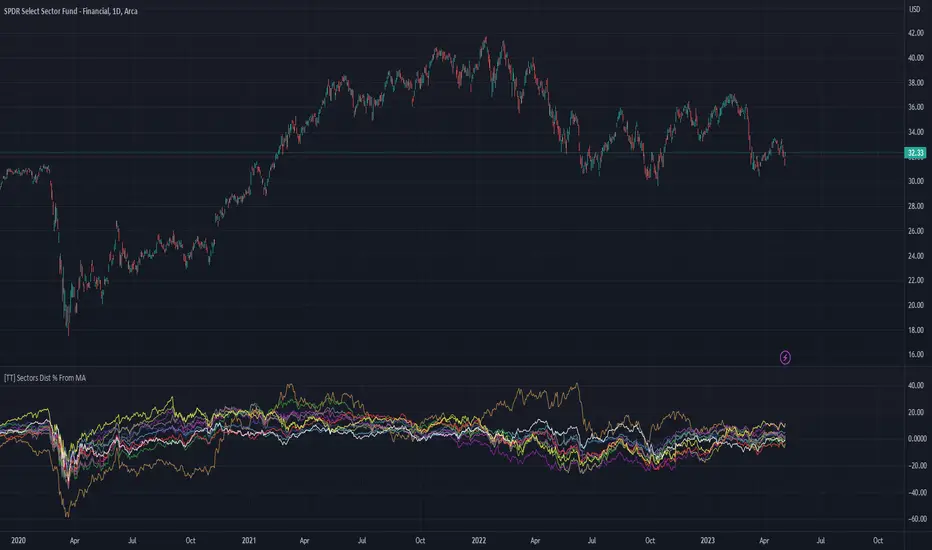
[TT] Sectors Dist % From MA- The script shows the distance in percentages from the 200 MA (or any other MA period) , for the 11 SP500 sectors.
- It works based on the current time frames.
Could be useful when working with mean reversion strategies to detect extremes zones and overbought/oversold conditions in the given sectors compared others.
LNL Keltner CandlesLNL Keltner Candles
This indicator plots mean reversion (reversal) arrows with custom painted candles based on the price touch or close above or below keltner channel limits (upper & lower bands). This study was created primarily for swing trading & higher time frames such as daily and weekly. Lower time frames might result in more false signals.
Mean Reversal Arrows:
1. Reversal Arrow Up - If the price drops below the lower band extremes, reversal up is the trigger for a bullish mean reversion.
2. Reversal Arrow Down - Once the price reach the higher band extremes, reversal down is the trigger for a bearish mean reversion.
The Concept of Mean Reversion:
There are just two types of moves in any market: The market is either expanding from the mean or retracing back to the mean. These reversions & epxansions are happening across all types of markets. The goal of this study is to catch the powerful mean reversion from extremes back to the mean. Once the candles light up green / red, it is time to look for the reversal (purple) arrow which triggers the mean reversion setup. Mean reversion is not about catching the next big swing turn to new highs or lows. It is all about the base hits = the mean. So the target here is always the average price. The idea here is to catch the average market ebbs & flows, not the next home run.
What Do I Mean by Mean?
Mean is usually the average price from the last 20-30 bars. Basically something like a 20 MA or Keltner Channel or Bollinger Band midline are really good visual representators of the mean (average price).
Hope it helps.

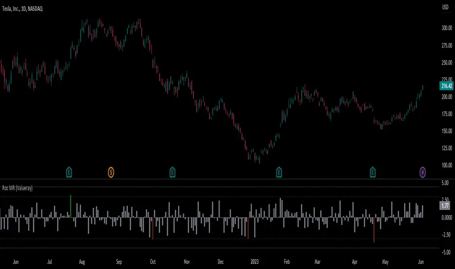
Roc Mean Reversion (ValueRay)This Indicator shows the Absolute Rate of Change in correlation to its Moving Average.
Values over 3 (gray dotted line) can savely be considered as a breakout; values over 4.5 got a high mean-reverting chance (red dotted line).
This Indicator can be used in all timeframes, however, i recommend to use it <30m, when you want search for meaningful Mean-Reverting Signals.
Please like, share and subscribe. With your love, im encouraged to write and publish more Indicators.
YJ Mean ReversionMean reversion strategy, based upon the price deviation (%) from a chosen moving average (bars). Do note that the "gains" are always relative to your starting capital, so if you set a smaller starting capital (e.g. $10000) your gains will look bigger. Also when the strategy tester has finished calculating, check the "Open P/L", as there could still be open trades.
Some Tips:
- Was designed firstly to work on an index like the S&P 500 , which over time tends to go up in value.
- Avoid trading too frequently (e.g. Daily, Weekly), to avoid getting eaten by fees.
- If you change the underlying asset, or time frame, tweaking the moving average may be necessary.
- Can work with a starting capital of just $1000, optimise the settings as necessary.
- Accepts floating point values for the amount of units to purchase (e.g. Bitcoin ).
- If price of units exceeds available capital, script will cancel the buy.
- Adjusted the input parameters to be more intuitive.
