Multi-TF Gates (Labels + Alerts)//@version=6
indicator("PO9 – Multi-TF Gates (Labels + Alerts)", overlay=true, max_lines_count=500)
iYear=input.int(2024,"Anchor Year",minval=1970)
iMonth=input.int(11,"Anchor Month",minval=1,maxval=12)
iDay=input.int(6,"Anchor Day",minval=1,maxval=31)
useSymbolTZ=input.bool(true,"Use symbol's exchange timezone (syminfo.timezone)")
tzChoice=input.string("Etc/UTC","Custom timezone (if not using symbol TZ)",options= )
anchorType=input.string("FX NY 17:00","Anchor at",options= )
showEvery=input.int(9,"Mark every Nth candle",minval=1)
showD=input.bool(true,"Show Daily")
show3H=input.bool(true,"Show 3H")
show1H=input.bool(true,"Show 1H")
show15=input.bool(true,"Show 15M")
show5=input.bool(false,"Show 5M (optional)")
colD=input.color(color.new(color.red,0),"Daily color")
col3H=input.color(color.new(color.orange,0),"3H color")
col1H=input.color(color.new(color.yellow,0),"1H color")
col15=input.color(color.new(color.teal,0),"15M color")
col5=input.color(color.new(color.gray,0),"5M color")
styStr=input.string("dashed","Line style",options= )
lnW=input.int(2,"Line width",minval=1,maxval=4)
extendTop=input.float(1.5,"ATR multiples above high",minval=0.1)
extendBottom=input.float(1.5,"ATR multiples below low",minval=0.1)
showLabels=input.bool(true,"Show labels")
enableAlerts=input.bool(true,"Enable alerts")
f_style(s)=>s=="solid"?line.style_solid:s=="dashed"?line.style_dashed:line.style_dotted
var lines=array.new_line()
f_prune(maxKeep)=>
if array.size(lines)>maxKeep
old=array.shift(lines)
line.delete(old)
tzEff=useSymbolTZ?syminfo.timezone:tzChoice
anchorTs=anchorType=="FX NY 17:00"?timestamp("America/New_York",iYear,iMonth,iDay,17,0):timestamp(tzEff,iYear,iMonth,iDay,0,0)
atr=ta.atr(14)
f_vline(_color,_tf,_idx)=>
y1=low-atr*extendBottom
y2=high+atr*extendTop
lid=line.new(x1=bar_index,y1=y1,x2=bar_index,y2=y2,xloc=xloc.bar_index,extend=extend.none,color=_color,style=f_style(styStr),width=lnW)
if showLabels
label.new(x=bar_index,y=high+(atr*2),text=_tf+" #"+str.tostring(_idx),xloc=xloc.bar_index,style=label.style_label_down,color=_color,textcolor=color.black)
array.push(lines,lid)
is_tf_open(tf)=> time==request.security(syminfo.tickerid,tf,time,barmerge.gaps_off,barmerge.lookahead_off)
f_tf(_tf,_show,_color,_name)=>
var bool started=false
var int idx=0
isOpen=_show and is_tf_open(_tf)
firstBar=isOpen and (time>=anchorTs) and (nz(time ,time)
Search in scripts for "股价站上60月线"

Opening Range Breakout with Multi-Timeframe Liquidity]═══════════════════════════════════════
OPENING RANGE BREAKOUT WITH MULTI-TIMEFRAME LIQUIDITY
═══════════════════════════════════════
A professional Opening Range Breakout (ORB) indicator enhanced with multi-timeframe liquidity detection, trading session visualization, volume analysis, and trend confirmation tools. Designed for intraday trading with comprehensive alert system.
───────────────────────────────────────
WHAT THIS INDICATOR DOES
───────────────────────────────────────
This indicator combines multiple trading concepts:
- Opening Range Breakout (ORB) - Customizable time period detection with automatic high/low identification
- Multi-Timeframe Liquidity - HTF (Higher Timeframe) and LTF (Lower Timeframe) key level detection
- Trading Sessions - Tokyo, London, New York, and Sydney session visualization
- Volume Analysis - Volume spike detection and strength measurement
- Multi-Timeframe Confirmation - Trend bias from higher timeframes
- EMA Integration - Trend filter and dynamic support/resistance
- Smart Alerts - Quality-filtered breakout notifications
───────────────────────────────────────
HOW IT WORKS
───────────────────────────────────────
OPENING RANGE BREAKOUT (ORB):
Concept:
The Opening Range is a period at the start of a trading session where price establishes an initial high and low. Breakouts beyond this range often indicate the direction of the day's trend.
Detection Method:
- Default: 15-minute opening range (configurable)
- Custom Range: Set specific session times with timezone support
- Automatically identifies ORH (Opening Range High) and ORL (Opening Range Low)
- Tracks ORB mid-point for reference
Range Establishment:
1. Session starts (or custom time begins)
2. Tracks highest high and lowest low during the period
3. Range confirmed at end of opening period
4. Levels extend throughout the session
Breakout Detection:
- Bullish Breakout: Close above ORH
- Bearish Breakout: Close below ORL
- Mid-point acts as bias indicator
Visual Display:
- Shaded box during range formation
- Horizontal lines for ORH, ORL, and mid-point
- Labels showing level values
- Color-coded fills based on selected method
Fill Color Methods:
1. Session Comparison:
- Green: Current OR mid > Previous OR mid
- Red: Current OR mid < Previous OR mid
- Gray: Equal or first session
- Shows day-over-day momentum
2. Breakout Direction (Recommended):
- Green: Price currently above ORH (bullish breakout)
- Red: Price currently below ORL (bearish breakout)
- Gray: Price inside range (no breakout)
- Real-time breakout status
MULTI-TIMEFRAME LIQUIDITY:
Two-Tier System for comprehensive level identification:
HTF (Higher Timeframe) Key Liquidity:
- Default: 4H timeframe (configurable to Daily, Weekly)
- Identifies major institutional levels
- Uses pivot detection with adjustable parameters
- Suitable for swing highs/lows where large orders rest
LTF (Lower Timeframe) Key Liquidity:
- Default: 1H timeframe (configurable)
- Provides precision entry/exit levels
- Finer granularity for intraday trading
- Captures minor swing points
Calculation Method:
- Pivot high/low detection algorithm
- Configurable left bars (lookback) and right bars (confirmation)
- Timeframe multiplier for accurate multi-timeframe detection
- Automatic level extension
Mitigation System:
- Tracks when levels are swept (broken)
- Configurable mitigation type: Wick or Close-based
- Option to remove or show mitigated levels
- Display limit prevents chart clutter
Asset-Specific Optimization:
The indicator includes quick reference settings for different assets:
- Major Forex (EUR/USD, GBP/USD): Default settings optimal
- Crypto (BTC/ETH): Left=12, Right=4, Display=7
- Gold: HTF=1D, Left=20
TRADING SESSIONS:
Four Major Sessions with Full Customization:
Tokyo Session:
- Default: 04:00-13:00 UTC+4
- Asian trading hours
- Often sets daily range
London Session:
- Default: 11:00-20:00 UTC+4
- Highest liquidity period
- Major institutional activity
New York Session:
- Default: 16:00-01:00 UTC+4
- US market hours
- High-impact news events
Sydney Session:
- Default: 01:00-10:00 UTC+4
- Earliest Asian activity
- Lower volatility
Session Features:
- Shaded background boxes
- Session name labels
- Optional open/close lines
- Session high/low tracking with colored lines
- Each session has independent color settings
- Fully customizable times and timezones
VOLUME ANALYSIS:
Volume-Based Trade Confirmation:
Volume MA:
- Configurable period (default: 20)
- Establishes average volume baseline
- Used for spike detection
Volume Spike Detection:
- Identifies when volume exceeds MA * multiplier
- Default: 1.5x average volume
- Confirms breakout strength
Volume Strength Measurement:
- Calculates current volume as percentage of average
- Shows relative volume intensity
- Used in alert quality filtering
High Volume Bars:
- Identifies bars above 50th percentile
- Additional confirmation layer
- Indicates institutional participation
MULTI-TIMEFRAME CONFIRMATION:
Trend Bias from Higher Timeframes:
HTF 1 (Trend):
- Default: 1H timeframe
- Uses EMA to determine intermediate trend
- Compares current timeframe EMA to HTF EMA
HTF 2 (Bias):
- Default: 4H timeframe
- Uses 50 EMA for longer-term bias
- Confirms overall market direction
Bias Classifications:
- Bullish Bias: HTF close > HTF 50 EMA AND Current EMA > HTF1 EMA
- Bearish Bias: HTF close < HTF 50 EMA AND Current EMA < HTF1 EMA
- Neutral Bias: Mixed signals between timeframes
EMA Stack Analysis:
- Compares EMA alignment across timeframes
- +1: Bullish stack (lower TF EMA > higher TF EMA)
- -1: Bearish stack (lower TF EMA < higher TF EMA)
- 0: Neutral/crossed
Usage:
- Filters false breakouts
- Confirms trend direction
- Improves trade quality
EMA INTEGRATION:
Dynamic EMA for Trend Reference:
Features:
- Configurable period (default: 20)
- Customizable color and width
- Acts as dynamic support/resistance
- Trend filter for ORB trades
Application:
- Above EMA: Favor long breakouts
- Below EMA: Favor short breakouts
- EMA cross: Potential trend change
- Distance from EMA: Momentum gauge
SMART ALERT SYSTEM:
Quality-Filtered Breakout Notifications:
Alert Types:
1. Standard ORB Breakout
2. High Quality ORB Breakout
Quality Criteria:
- Volume Confirmation: Volume > 1.2x average
- MTF Confirmation: Bias aligned with breakout direction
Standard Alert:
- Basic breakout detection
- Price crosses ORH or ORL
- Icon: 🚀 (bullish) or 🔻 (bearish)
High Quality Alert:
- Both volume AND MTF confirmed
- Stronger probability setup
- Icon: 🚀⭐ (bullish) or 🔻⭐ (bearish)
Alert Information Includes:
- Alert quality rating
- Breakout level and current price
- Volume strength percentage (if enabled)
- MTF bias status (if enabled)
- Recommended action
One Alert Per Bar:
- Prevents alert spam
- Uses flag system to track sent alerts
- Resets on new ORB session
───────────────────────────────────────
HOW TO USE
───────────────────────────────────────
OPENING RANGE SETUP:
Basic Configuration:
1. Select time period for opening range (default: 15 minutes)
2. Choose fill color method (Breakout Direction recommended)
3. Enable historical data display if needed
Custom Range (Advanced):
1. Enable Custom Range toggle
2. Set specific session time (e.g., 0930-0945)
3. Select appropriate timezone
4. Useful for specific market opens (NYSE, LSE, etc.)
LIQUIDITY LEVELS SETUP:
Quick Configuration by Asset:
- Forex: Use default settings (Left=15, Right=5)
- Crypto: Set Left=12, Right=4, Display=7
- Gold: Set HTF=1D, Left=20
HTF Liquidity:
- Purpose: Major support/resistance levels
- Recommended: 4H for day trading, 1D for swing trading
- Use as profit targets or reversal zones
LTF Liquidity:
- Purpose: Entry/exit refinement
- Recommended: 1H for day trading, 4H for swing trading
- Use for position management
Mitigation Settings:
- Wick-based: More sensitive (default)
- Close-based: More conservative
- Remove or Show mitigated levels based on preference
TRADING SESSIONS SETUP:
Enable/Disable Sessions:
- Master toggle for all sessions
- Individual session controls
- Show/hide session names
Session High/Low Lines:
- Enable to see session extremes
- Each session has custom colors
- Useful for range trading
Customization:
- Adjust session times for your broker
- Set timezone to match your location
- Customize colors for visibility
VOLUME ANALYSIS SETUP:
Enable Volume Analysis:
1. Toggle on Volume Analysis
2. Set MA length (20 recommended)
3. Adjust spike multiplier (1.5 typical)
Usage:
- Confirm breakouts with volume
- Identify climactic moves
- Filter false signals
MULTI-TIMEFRAME SETUP:
HTF Selection:
- HTF 1 (Trend): 1H for day trading, 4H for swing
- HTF 2 (Bias): 4H for day trading, 1D for swing
Interpretation:
- Trade only with bias alignment
- Neutral bias: Be cautious
- Bias changes: Potential reversals
EMA SETUP:
Configuration:
- Period: 20 for responsive, 50 for smoother
- Color: Choose contrasting color
- Width: 1-2 for visibility
Usage:
- Filter trades: Long above, Short below
- Dynamic support/resistance reference
- Trend confirmation
ALERT SETUP:
TradingView Alert Creation:
1. Enable alerts in indicator settings
2. Enable ORB Breakout Alerts
3. Right-click chart → Add Alert
4. Select this indicator
5. Choose "Any alert() function call"
6. Configure delivery method (mobile, email, webhook)
Alert Filtering:
- All alerts include quality rating
- High Quality alerts = Volume + MTF confirmed
- Standard alerts = Basic breakout only
───────────────────────────────────────
TRADING STRATEGIES
───────────────────────────────────────
CLASSIC ORB STRATEGY:
Setup:
1. Wait for opening range to complete
2. Price breaks and closes above ORH or below ORL
3. Volume > average (if enabled)
4. MTF bias aligned (if enabled)
Entry:
- Bullish: Buy on break above ORH
- Bearish: Sell on break below ORL
- Consider retest entries for better risk/reward
Stop Loss:
- Bullish: Below ORL or range mid-point
- Bearish: Above ORH or range mid-point
- Adjust based on volatility
Targets:
- Initial: Range width extension (ORH + range width)
- Secondary: HTF liquidity levels
- Final: Session high/low or major support/resistance
ORB + LIQUIDITY CONFLUENCE:
Enhanced Setup:
1. Opening range established
2. HTF liquidity level near or beyond ORH/ORL
3. Breakout occurs with volume
4. Price targets the liquidity level
Entry:
- Enter on ORB breakout
- Target the HTF liquidity level
- Use LTF liquidity for position management
Management:
- Partial profits at ORB + range width
- Move stop to breakeven at LTF liquidity
- Final exit at HTF liquidity sweep
ORB REJECTION STRATEGY (Counter-Trend):
Setup:
1. Price breaks above ORH or below ORL
2. Weak volume (below average)
3. MTF bias opposite to breakout
4. Price closes back inside range
Entry:
- Failed bullish break: Short below ORH
- Failed bearish break: Long above ORL
Stop Loss:
- Beyond the failed breakout level
- Or beyond session extreme
Target:
- Opposite end of opening range
- Range mid-point for partial profit
SESSION-BASED ORB TRADING:
Tokyo Session:
- Typically narrower ranges
- Good for range trading
- Wait for London open breakout
London Session:
- Highest volume and volatility
- Strong ORB setups
- Major liquidity sweeps common
New York Session:
- Strong trending moves
- News-driven volatility
- Good for momentum trades
Sydney Session:
- Quieter conditions
- Suitable for range strategies
- Sets up Tokyo session
EMA-FILTERED ORB:
Rules:
- Only take bullish breaks if price > EMA
- Only take bearish breaks if price < EMA
- Ignore counter-trend breaks
Benefits:
- Reduces false signals
- Aligns with larger trend
- Improves win rate
───────────────────────────────────────
CONFIGURATION GUIDE
───────────────────────────────────────
OPENING RANGE SETTINGS:
Time Period:
- 15 min: Standard for most markets
- 30 min: Wider range, fewer breakouts
- 60 min: For slower markets or swing trades
Custom Range:
- Use for specific market opens
- NYSE: 0930-1000 EST
- LSE: 0800-0830 GMT
- Set timezone to match exchange
Historical Display:
- Enable: See all previous session data
- Disable: Cleaner chart, current session only
LIQUIDITY SETTINGS:
Left Bars (5-30):
- Lower: More frequent, sensitive levels
- Higher: Fewer, more significant levels
- Recommended: 15 for most markets
Right Bars (1-25):
- Confirmation period
- Higher: More reliable, less frequent
- Recommended: 5 for balance
Display Limit (1-20):
- Number of active levels shown
- Higher: More context, busier chart
- Recommended: 7 for clarity
Extension Options:
- Short: Levels visible near formation
- Current: Extended to current bar (recommended)
- Max: Extended indefinitely
VOLUME SETTINGS:
MA Length (5-50):
- Shorter: More responsive to spikes
- Longer: Smoother baseline
- Recommended: 20 for balance
Spike Multiplier (1.0-3.0):
- Lower: More sensitive spike detection
- Higher: Only extreme spikes
- Recommended: 1.5 for day trading
MULTI-TIMEFRAME SETTINGS:
HTF 1 (Trend):
- 5m chart: Use 15m or 1H
- 15m chart: Use 1H or 4H
- 1H chart: Use 4H or 1D
HTF 2 (Bias):
- One level higher than HTF 1
- Provides longer-term context
- Don't use same as HTF 1
EMA SETTINGS:
Length:
- 20: Responsive, more signals
- 50: Smoother, stronger filter
- 200: Long-term trend only
Style:
- Choose contrasting color
- Width 1-2 for visibility
- Match your trading style
───────────────────────────────────────
BEST PRACTICES
───────────────────────────────────────
Chart Timeframe Selection:
- ORB Trading: Use 5m or 15m charts
- Session Review: Use 1H or 4H charts
- Swing Trading: Use 1H or 4H charts
Quality Over Quantity:
- Wait for high-quality alerts (volume + MTF)
- Avoid trading every breakout
- Focus on confluence setups
Risk Management:
- Position size based on range width
- Wider ranges = smaller positions
- Use stop losses always
- Take partial profits at targets
Market Conditions:
- Best results in trending markets
- Reduce position size in choppy conditions
- Consider session overlaps for volatility
- Avoid trading near major news if inexperienced
Continuous Improvement:
- Track win rate by session
- Note which confluence factors work best
- Adjust settings based on market volatility
- Review performance weekly
───────────────────────────────────────
PERFORMANCE OPTIMIZATION
───────────────────────────────────────
This indicator is optimized with:
- max_bars_back declarations for efficient processing
- Conditional calculations based on enabled features
- Proper memory management for drawing objects
- Minimal recalculation on each bar
Best Practices:
- Disable unused features (sessions, MTF, volume)
- Limit historical display to reduce rendering
- Use appropriate timeframe for your strategy
- Clear old drawing objects periodically
───────────────────────────────────────
EDUCATIONAL DISCLAIMER
───────────────────────────────────────
This indicator combines established trading concepts:
- Opening Range Breakout theory (price action)
- Liquidity level detection (pivot analysis)
- Session-based trading (time-of-day patterns)
- Volume analysis (confirmation technique)
- Multi-timeframe analysis (trend alignment)
All calculations use standard technical analysis methods:
- Pivot high/low detection algorithms
- Moving averages for trend and volume
- Session time filtering
- Timeframe security functions
The indicator identifies potential trading setups but does not predict future price movements. Success requires proper application within a complete trading strategy including risk management, position sizing, and market context.
───────────────────────────────────────
USAGE DISCLAIMER
───────────────────────────────────────
This tool is for educational and analytical purposes. Opening Range Breakout trading involves substantial risk. The alert system and quality filters are designed to identify potential setups but do not guarantee profitability. Always conduct independent analysis, use proper risk management, and never risk capital you cannot afford to lose. Past performance does not indicate future results. Trading intraday breakouts requires experience and discipline.
───────────────────────────────────────
CREDITS & ATTRIBUTION
───────────────────────────────────────
ORIGINAL SOURCE:
This indicator builds upon concepts from LuxAlgo's-ORB

OPADA//@version=5
indicator("Buy/Sell Zones – TV Style", overlay=true, timeframe="", timeframe_gaps=true)
//=====================
// الإعدادات
//=====================
len = input.int(100, "Length", minval=10)
useATR = input.bool(true, "Use ATR (بدل الانحراف المعياري)")
mult = input.float(2.0, "Band Multiplier", step=0.1)
useRSI = input.bool(true, "تفعيل فلتر RSI")
rsiOB = input.int(70, "RSI Overbought", minval=50, maxval=90)
rsiOS = input.int(30, "RSI Oversold", minval=10, maxval=50)
//=====================
// القناة: أساس + انحراف
//=====================
basis = ta.linreg(close, len, 0)
off = useATR ? ta.atr(len) * mult : ta.stdev(close, len) * mult
upper = basis + off
lower = basis - off
// نطاق علوي/سفلي بعيد لعمل تعبئة المناطق
lookback = math.min(bar_index, 500)
topBand = ta.highest(high, lookback) + 50 * syminfo.mintick
bottomBand = ta.lowest(low, lookback) - 50 * syminfo.mintick
//=====================
// الرسم
//=====================
pUpper = plot(upper, "Upper", color=color.new(color.blue, 0), linewidth=1)
pLower = plot(lower, "Lower", color=color.new(color.red, 0), linewidth=1)
pBasis = plot(basis, "Basis", color=color.new(color.gray, 60), linewidth=2)
// تعبئة المناطق: فوق القناة (أزرق)، تحت القناة (أحمر)
pTop = plot(topBand, display=display.none)
pBottom = plot(bottomBand, display=display.none)
fill(pUpper, pTop, color=color.new(color.blue, 80)) // منطقة مقاومة/بيع
fill(pBottom, pLower, color=color.new(color.red, 80)) // منطقة دعم/شراء
//=====================
// خط أفقي من قمّة قريبة (يمثل مقاومة) – قريب من الخط المنقّط في الصورة
//=====================
resLen = math.round(len * 0.6)
dynRes = ta.highest(high, resLen)
plot(dynRes, "Recent Resistance", color=color.new(color.white, 0), linewidth=1)
//=====================
// إشارات BUY / SELL + فلتر RSI (اختياري)
//=====================
rsi = ta.rsi(close, 14)
touchLower = ta.crossover(close, lower) or close <= lower
touchUpper = ta.crossunder(close, upper) or close >= upper
buyOK = useRSI ? (touchLower and rsi <= rsiOS) : touchLower
sellOK = useRSI ? (touchUpper and rsi >= rsiOB) : touchUpper
plotshape(buyOK, title="BUY", location=location.belowbar, style=shape.labelup,
text="BUY", color=color.new(color.green, 0), textcolor=color.white, size=size.tiny, offset=0)
plotshape(sellOK, title="SELL", location=location.abovebar, style=shape.labeldown,
text="SELL", color=color.new(color.red, 0), textcolor=color.white, size=size.tiny, offset=0)
// تنبيهات
alertcondition(buyOK, title="BUY", message="BUY signal: price touched/closed below lower band (RSI filter may apply).")
alertcondition(sellOK, title="SELL", message="SELL signal: price touched/closed above upper band (RSI filter may apply).")

Buy/Sell Zones – TV Style//@version=5
indicator("Buy/Sell Zones – TV Style", overlay=true, timeframe="", timeframe_gaps=true)
//=====================
// الإعدادات
//=====================
len = input.int(100, "Length", minval=10)
useATR = input.bool(true, "Use ATR (بدل الانحراف المعياري)")
mult = input.float(2.0, "Band Multiplier", step=0.1)
useRSI = input.bool(true, "تفعيل فلتر RSI")
rsiOB = input.int(70, "RSI Overbought", minval=50, maxval=90)
rsiOS = input.int(30, "RSI Oversold", minval=10, maxval=50)
//=====================
// القناة: أساس + انحراف
//=====================
basis = ta.linreg(close, len, 0)
off = useATR ? ta.atr(len) * mult : ta.stdev(close, len) * mult
upper = basis + off
lower = basis - off
// نطاق علوي/سفلي بعيد لعمل تعبئة المناطق
lookback = math.min(bar_index, 500)
topBand = ta.highest(high, lookback) + 50 * syminfo.mintick
bottomBand = ta.lowest(low, lookback) - 50 * syminfo.mintick
//=====================
// الرسم
//=====================
pUpper = plot(upper, "Upper", color=color.new(color.blue, 0), linewidth=1)
pLower = plot(lower, "Lower", color=color.new(color.red, 0), linewidth=1)
pBasis = plot(basis, "Basis", color=color.new(color.gray, 60), linewidth=2)
// تعبئة المناطق: فوق القناة (أزرق)، تحت القناة (أحمر)
pTop = plot(topBand, display=display.none)
pBottom = plot(bottomBand, display=display.none)
fill(pUpper, pTop, color=color.new(color.blue, 80)) // منطقة مقاومة/بيع
fill(pBottom, pLower, color=color.new(color.red, 80)) // منطقة دعم/شراء
//=====================
// خط أفقي من قمّة قريبة (يمثل مقاومة) – قريب من الخط المنقّط في الصورة
//=====================
resLen = math.round(len * 0.6)
dynRes = ta.highest(high, resLen)
plot(dynRes, "Recent Resistance", color=color.new(color.white, 0), linewidth=1)
//=====================
// إشارات BUY / SELL + فلتر RSI (اختياري)
//=====================
rsi = ta.rsi(close, 14)
touchLower = ta.crossover(close, lower) or close <= lower
touchUpper = ta.crossunder(close, upper) or close >= upper
buyOK = useRSI ? (touchLower and rsi <= rsiOS) : touchLower
sellOK = useRSI ? (touchUpper and rsi >= rsiOB) : touchUpper
plotshape(buyOK, title="BUY", location=location.belowbar, style=shape.labelup,
text="BUY", color=color.new(color.green, 0), textcolor=color.white, size=size.tiny, offset=0)
plotshape(sellOK, title="SELL", location=location.abovebar, style=shape.labeldown,
text="SELL", color=color.new(color.red, 0), textcolor=color.white, size=size.tiny, offset=0)
// تنبيهات
alertcondition(buyOK, title="BUY", message="BUY signal: price touched/closed below lower band (RSI filter may apply).")
alertcondition(sellOK, title="SELL", message="SELL signal: price touched/closed above upper band (RSI filter may apply).")

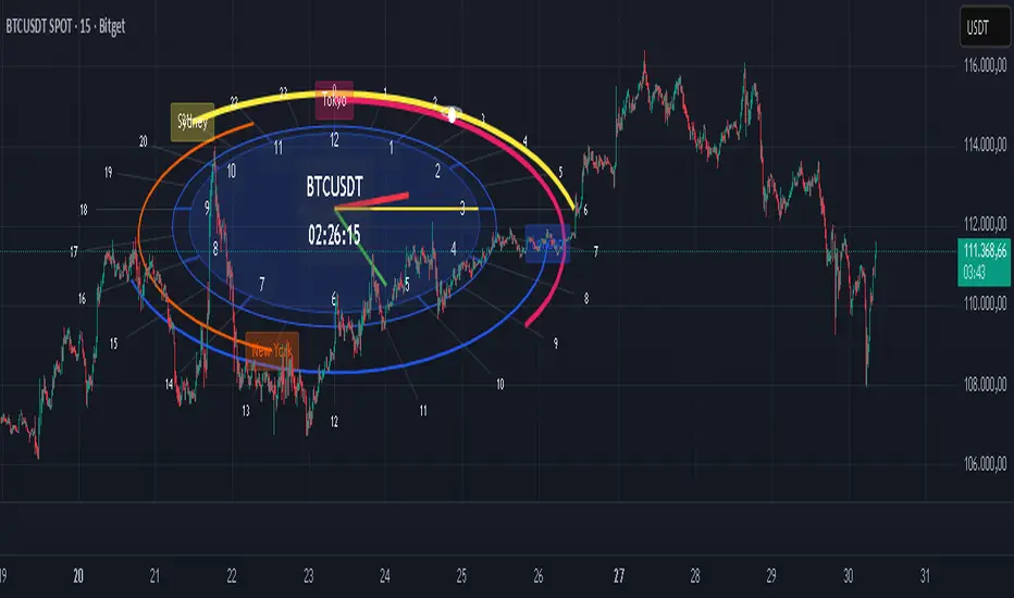
3D Session Clock | Live Time with Sessions [CHE] 3D Session Clock | Live Time with Sessions — Projects a perspective clock face onto the chart to display current time and market session periods for enhanced situational awareness during trading hours.
Summary
This indicator renders a three-dimensional clock projection directly on the price chart, showing analog hands for hours, minutes, and seconds alongside a digital time readout. It overlays session arcs for major markets like New York, London, Tokyo, and Sydney, highlighting the active one with thicker lines and contrasting labels. By centralizing time and session visibility, it reduces the need to reference external clocks, allowing traders to maintain focus on price action while noting overlaps or transitions that influence volatility.
The design uses perspective projection to simulate depth, making the clock appear tilted for better readability on varying chart scales. Sessions are positioned radially outward from the main clock, with the current time marker pulsing on the relevant arc. This setup provides a static yet live-updating view, confirmed on bar close to avoid intrabar shifts.
Motivation: Why this design?
Traders often miss subtle session shifts amid fast-moving charts, leading to entries during low-liquidity periods or exits before peak activity. Standard chart tools lack integrated time visualization, forcing constant tab-switching. This indicator addresses that by embedding a customizable clock with session rings, ensuring time context is always in view without disrupting workflow.
What’s different vs. standard approaches?
- Reference baseline: Traditional session highlighters use simple background fills or vertical lines, which clutter the chart and ignore global time zones.
- Architecture differences:
- Perspective projection rotates and scales points to mimic 3D depth, unlike flat 2D drawings.
- Nested radial arcs for sessions, with dynamic radius assignment to avoid overlap.
- Live time calculation adjusted for user-selected time zones, including optional daylight savings offset.
- Practical effect: The tilted view prevents labels from bunching at chart edges, and active session emphasis draws the eye to liquidity hotspots, making multi-session overlaps immediately apparent for better timing.
How it works (technical)
The indicator calculates current time in the selected time zone by adjusting the system timestamp with a fixed offset, plus an optional one-hour bump for daylight savings. This yields hour, minute, and second values that drive hand positions: the hour hand advances slowly with fractional minute input, the minute hand ticks per 60 seconds, and the second hand sweeps fully each minute.
Points for the clock face and arcs are generated as arrays of coordinates, transformed via rotation around the x-axis to apply tilt, then projected onto chart space using a scaling factor based on depth. Radial lines mark every hour from zero to 23, extending to the outermost session ring. Session arcs span user-defined hour ranges, drawn as open polylines with step interpolation for smoothness.
On the last bar, all prior drawings are cleared, and new elements are added: filled clock circles, hand lines from center to tip, a small orbiting circle at the current time position, and centered labels for hours, sessions, and time. The active session is identified by checking if the current time falls within its range, then its arc thickens and label inverts colors. Initialization populates a timezone array once, with persistent bar time tracking for horizontal positioning.
Parameter Guide
Clock Size — Controls overall radius in pixels, affecting visibility on dense charts — Default: 200 — Larger values suit wide screens but may crowd small views; start smaller for mobile.
Camera Angle — Sets tilt from top-down (zero) to side (90 degrees), altering projection depth — Default: 45 — Steeper angles enhance readability on sloped trends but flatten at extremes.
Resolution — Defines polygon sides for circles and arcs, balancing smoothness and draw calls — Default: 64 — Higher improves curves on large clocks; lower aids performance on slow devices.
Hour/Minute/Second Hand Length — Scales each hand from center, with seconds longest for precision — Defaults: 100/150/180 — Proportional sizing prevents overlap; shorten for compact layouts.
Clock Base Color — Tints face and frame — Default: blue — Neutral shades reduce eye strain; match chart theme.
Hand Colors — Assigns distinct hues to each hand — Defaults: red/green/yellow — High contrast aids quick scans; avoid chart-matching to stand out.
Hour Label Size — Text scale for 1-12 markers — Default: normal — Larger for distant views, but risks clutter.
Digital Time Size — Scale for HH:MM:SS readout — Default: large — Matches clock for balance; tiny for minimalism.
Digital Time Vertical Offset — Shifts readout up (negative) or down — Default: -50 — Positions above clock to avoid hand interference.
Timezone — Selects reference city/offset — Default: New York (UTC-05) — Matches trading locale; verify offsets manually.
Summer Time (DST) — Adds one hour if active — Default: false — Enable for regions observing it; test transitions.
Show/Label/Session/Color for Each Market — Toggles arc, sets name, time window, and hue per session (New York/London/Tokyo/Sydney) — Defaults: true/"New York"/1300-2200/orange, etc. — Customize windows to local exchange hours; colors differentiate overlaps.
Reading & Interpretation
The analog face shows a blue-tinted circle with white 1-12 labels and gray hour ticks; hands extend from center in assigned colors, pointing to current positions. A white dot with orbiting ring marks exact time on the session arc. Digital readout below displays padded HH:MM:SS in white on black.
Active sessions glow with bold arcs and white labels on colored backgrounds; inactive ones use thin lines and colored text on light fills. Overlaps stack outward, with the innermost (New York) closest to the clock. If no session is active, the marker sits on the base ring.
Practical Workflows & Combinations
- Trend following: Enter longs during London-New York overlap (thicker dual arcs) confirmed by higher highs; filter with volume spikes.
- Exits/Stops: Tighten stops pre-Tokyo open if arc thickens, signaling volatility ramp; trail during Sydney for overnight holds.
- Multi-asset/Multi-TF: Defaults work across forex/stocks; on higher timeframes, enlarge clock size to counter bar spacing. Pair with session volume oscillators for confirmation.
Behavior, Constraints & Performance
Rendering occurs only on the last bar, using confirmed history for stable display; live bars update hands and marker without repainting prior elements. No security calls or higher timeframe fetches, so no lookahead bias.
Resource limits include 2000 bars back for positioning, 500 each for lines, labels, and boxes—sufficient for full sessions without overflow. Arrays hold timezone data statically. On very wide charts, projection may skew slightly due to fixed scale.
Known limits: Visual positioning drifts on extreme zooms; daylight savings assumes manual toggle, risking one-hour errors during changes.
Sensible Defaults & Quick Tuning
Start with New York timezone, 45-degree tilt, and all sessions enabled—these balance global coverage without clutter. For too-small visibility, bump clock size to 300 and resolution to 48. If labels overlap on narrow views, reduce hand lengths proportionally. To emphasize one session (e.g., London), disable others and widen its color contrast. For minimalism, set digital size to small and offset to -100.
What this indicator is—and isn’t
This is a visual time and session overlay to contextualize trading windows, not a signal generator or predictive tool. It complements price analysis and risk rules but requires manual interpretation. Use alongside order flow or momentum indicators for decisions.
Disclaimer
The content provided, including all code and materials, is strictly for educational and informational purposes only. It is not intended as, and should not be interpreted as, financial advice, a recommendation to buy or sell any financial instrument, or an offer of any financial product or service. All strategies, tools, and examples discussed are provided for illustrative purposes to demonstrate coding techniques and the functionality of Pine Script within a trading context.
Any results from strategies or tools provided are hypothetical, and past performance is not indicative of future results. Trading and investing involve high risk, including the potential loss of principal, and may not be suitable for all individuals. Before making any trading decisions, please consult with a qualified financial professional to understand the risks involved.
By using this script, you acknowledge and agree that any trading decisions are made solely at your discretion and risk.
Do not use this indicator on Heikin-Ashi, Renko, Kagi, Point-and-Figure, or Range charts, as these chart types can produce unrealistic results for signal markers and alerts.
Best regards and happy trading
Chervolino
Acknowledgments
This indicator draws inspiration from the open-source contributions of the TradingView community, whose advanced programming techniques have greatly influenced its development. Special thanks to LonesomeTheBlue for the innovative polyline handling and midpoint centering techniques in RSI Radar Multi Time Frame:
Gratitude also extends to LuxAlgo for the precise timezone calculations in Sessions:
Finally, appreciation to TradingView for their comprehensive documentation on polyline features, including the support article at www.tradingview.com and the blog post at www.tradingview.com These resources were instrumental in implementing smooth, dynamic drawings.
Lot Size Calculator - Gold🥇 Lot Size Calculator for Gold (XAU/USD)
Description:
A professional and accurate lot size calculator specifically designed for Gold (XAU/USD) trading. This indicator helps traders calculate the optimal position size based on account balance, risk percentage, and stop loss distance, ensuring proper risk management for every trade.
Key Features:
Accurate Gold Calculations - Properly accounts for Gold pip values ($10 per pip for standard 100oz lots)
Multi-Currency Support - Works with USD, EUR, and GBP account currencies
Flexible Contract Sizes - Supports Standard (100 oz), Mini (10 oz), and Micro (1 oz) lots
Customizable Decimal Places - Display lot sizes with 2-8 decimal precision (no rounding)
Clean Visual Design - Modern, professional info panel with gold-themed styling
Adjustable Display - Position panel anywhere on chart with customizable colors and sizes
Real-Time Calculations - Instantly updates as you adjust your risk parameters
How It Works:
The calculator uses the standard forex position sizing formula optimized for Gold:
Lot Size = Risk Amount / (Stop Loss in Pips × Pip Value Per Lot)
For Gold (XAU/USD):
Standard Lot (100 oz): 1 pip = $10
Mini Lot (10 oz): 1 pip = $1
Micro Lot (1 oz): 1 pip = $0.10
Settings:
Account Settings:
Account Balance: Your trading capital
Account Currency: USD, EUR, or GBP
Risk Percentage: How much to risk per trade (default: 2%)
Contract Size: 100 oz (Standard), 10 oz (Mini), or 1 oz (Micro)
Display Currency: Choose how to display risk amounts
Trade Settings:
Stop Loss: Your SL distance in pips
Display Settings:
Label Position: Top/Bottom, Left/Right, Middle Right
Label Size: Tiny to Huge
Decimal Places: 2-8 decimals
Custom Colors: Background, text, and accent colors
Perfect For:
Gold (XAU/USD) day traders and swing traders
Position sizing and risk management
Traders using fixed percentage risk models
Anyone trading Gold CFDs or spot markets
Scalpers to long-term Gold investors
What Makes This Different:
Unlike generic lot size calculators, this tool correctly calculates Gold's pip values based on contract size. Many calculators get this wrong, leading to incorrect position sizing. This indicator ensures you're always trading the right lot size for your risk tolerance.
Example Usage:
Account Balance: $10,000
Risk: 1% = $100
Stop Loss: 60 pips
Contract Size: 100 oz (Standard)
Result: 0.1667 lots (exact, no rounding)
Perfect for maintaining consistent risk management in your Gold trading strategy!

cd_correlation_analys_Cxcd_correlation_analys_Cx
General:
This indicator is designed for correlation analysis by classifying stocks (487 in total) and indices (14 in total) traded on Borsa İstanbul (BIST) on a sectoral basis.
Tradingview's sector classifications (20) have been strictly adhered to for sector grouping.
Depending on user preference, the analysis can be performed within sectors, between sectors, or manually (single asset).
Let me express my gratitude to the code author, @fikira, beforehand; you will find the reason for my thanks in the context.
Details:
First, let's briefly mention how this indicator could have been prepared using the classic method before going into details.
Classically, assets could be divided into groups of forty (40), and the analysis could be performed using the built-in function:
ta.correlation(source1, source2, length) → series float.
I chose sectoral classification because I believe there would be a higher probability of assets moving together, rather than using fixed-number classes.
In this case, 21 arrays were formed with the following number of elements:
(3, 11, 21, 60, 29, 20, 12, 3, 31, 5, 10, 11, 6, 48, 73, 62, 16, 19, 13, 34 and indices (14)).
However, you might have noticed that some arrays have more than 40 elements. This is exactly where @Fikira's indicator came to the rescue. When I examined their excellent indicator, I saw that it could process 120 assets in a single operation. (I believe this was the first limit overrun; thanks again.)
It was amazing to see that data for 3 pairs could be called in a single request using a special method.
You can find the details here:
When I adapted it for BIST, I found it sufficient to call data for 2 pairs instead of 3 in a single go. Since asset prices are regular and have 2 decimal places, I used a fixed multiplier of $10^8$ and a fixed decimal count of 2 in Fikira's formulas.
With this method, the (high, low, open, close) values became accessible for each asset.
The summary up to this point is that instead of the ready-made formula + groups of 40, I used variable-sized groups and the method I will detail now.
Correlation/harmony/co-movement between assets provides advantages to market participants. Coherent assets are expected to rise or fall simultaneously.
Therefore, to convert co-movement into a mathematical value, I defined the possible movements of the current candle relative to the previous candle bar over a certain period (user-defined). These are:
Up := high > high and low > low
Down := high < high and low < low
Inside := high <= high and low >= low
Outside := high >= high and low <= low and NOT Inside.
Ignore := high = low = open = close
If both assets performed the same movement, 1 was added to the tracking counter.
If (Up-Up), (Down-Down), (Inside-Inside), or (Outside-Outside), then counter := counter + 1.
If the period length is 100 and the counter is 75, it means there is 75% co-movement.
Corr = counter / period ($75/100$)
Average = ta.sma(Corr, 100) is obtained.
The highest coefficients recorded in the array are presented to the user in a table.
From the user menu options, the user can choose to compare:
• With assets in its own sector
• With assets in the selected sector
• By activating the confirmation box and manually entering a single asset for comparison.
Table display options can be adjusted from the Settings tab.
In the attached examples:
Results for AKBNK stock from the Finance sector compared with GARAN stock from the same sector:
Timeframe: Daily, Period: 50 => Harmony 76% (They performed the same movement in 38 out of 50 bars)
Comment: Opposite movements at swing high and low levels may indicate a change in the direction of the price flow (SMT).
Looking at ASELS from the Electronic Technology sector over the last 30 daily candles, they performed the same movements by 40% with XU100, 73.3% (22/30) with XUTEK (Technology Index), and 86.9% according to the averages.
Comment: It is more appropriate to follow ASELS stock with XUTEK (Technology index) instead of the general index (XU100). Opposite movements at swing high and low levels may indicate a change in the direction of the price flow (SMT).
Again, when ASELS stock is taken on H1 instead of daily, and the length is 100 instead of 30, the harmony rate is seen to be 87%.
Please share your thoughts and criticisms regarding the indicator, which I prepared with a bit of an educational purpose specifically for BIST.
Happy trading.

Ultra-Fast Scalp Predictor 2This is a Pine Script (version 5) indicator engineered for ultra-low latency scalping, optimized specifically for very short timeframes (1-second to 1-minute charts) to predict price direction over the next 30-60 seconds.
It operates as a single, composite directional score by combining six highly sensitive, fast-moving analytical components.
Core Prediction Methodology:
The indicator calculates a single predictionScore which is a sum of six weighted factors, designed to capture immediate changes in market momentum, volatility, and order flow pressure.
The Prediction Score determines the signal:
predictUp: predictionScore is greater than the Bull Threshold ($\text{Sensitivity} \times 10$).
predictDown: predictionScore is less than the Bear Threshold ($\text{Sensitivity} \times -10$).
confidence: Calculated as the normalized absolute magnitude of the predictionScore relative to a theoretical maximum (math.abs(predictionScore) / 50 \times 100).

⚡ Zero-Lag 60s Binary Predictor🧠 Core Anti-Lag Philosophy
The indicator's primary goal is to overcome the inherent lag of traditional indicators like the Simple Moving Average (SMA) or standard Relative Strength Index (RSI). It achieves this by focusing on:
Leading Indicators: Using derivatives of price/momentum (like acceleration and jerk—the second and third derivatives of price) to predict turns before the price action is clear.
Instantaneous Metrics: Using short lookback periods (e.g., ta.change(close, 1) or fastLength = 5) and heavily weighting the most recent data (e.g., in instMomentum).
Market Microstructure: Incorporating metrics like Tick Pressure and Order Flow Imbalance (OFI), which attempt to measure internal bar dynamics and buying/selling aggression.
Zero-Lag Techniques: Specifically, the Ehlers Zero Lag EMA, which is mathematically constructed to eliminate phase lag by predicting where the price will be rather than where it was.

SB LONG ENTRY/EXITBASED on HULL slope average. ISN'T IT VERY ROBUST?
Very good for daily, weekly and monthly timeframes. Stocks especially.....
I prefer it without optonal stop loss on other position protection stops.
Wonderful both equal weight position or with a D'alembert style weighting of positions....
Hold the Hull period parameter between 30 and 60 or more, but it's not so sensitive to this optimization.
All the best,
Sandro Bisotti

Ehlers Ultrasmooth Filter (USF)# USF: Ultrasmooth Filter
## Overview and Purpose
The Ultrasmooth Filter (USF) is an advanced signal processing tool that represents the pinnacle of noise reduction technology for financial time series. Developed by John Ehlers, this filter implements a complex algorithm that provides exceptional smoothing capabilities while minimizing the lag typically associated with heavy filtering. USF builds upon the Super Smooth Filter (SSF) with enhanced noise suppression characteristics, making it particularly valuable for identifying clear trends in extremely noisy market conditions where even traditional smoothing techniques struggle to produce clean signals.
## Core Concepts
* **Maximum noise suppression:** Provides the highest level of noise reduction among Ehlers' filter designs
* **Optimized coefficient structure:** Uses carefully designed mathematical relationships to achieve superior filtering performance
* **Market application:** Particularly effective for long-term trend identification and minimizing false signals in highly volatile market conditions
The core innovation of USF is its second-order filter structure with optimized coefficients that create an exceptionally smooth frequency response. By careful mathematical design, USF achieves near-optimal noise suppression characteristics while minimizing the lag and waveform distortion that typically accompany such heavy filtering. This makes it especially valuable for identifying major market trends amid significant short-term volatility.
## Common Settings and Parameters
| Parameter | Default | Function | When to Adjust |
|-----------|---------|----------|---------------|
| Length | 20 | Controls the cutoff period | Increase for smoother signals, decrease for more responsiveness |
| Source | close | Price data used for calculation | Consider using hlc3 for a more balanced price representation |
**Pro Tip:** USF is ideal for defining major market trends - try using it with a length of 40-60 on daily charts to identify dominant market direction and ignoring shorter-term noise completely.
## Calculation and Mathematical Foundation
**Simplified explanation:**
The Ultrasmooth Filter creates an extremely clean price representation by combining current and past price data with previous filter outputs using precisely calculated mathematical relationships. This creates a highly effective "averaging" process that removes virtually all market noise while still maintaining the essential trend information.
**Technical formula:**
USF = (1-c1)X + (2c1-c2)X₁ - (c1+c3)X₂ + c2×USF₁ + c3×USF₂
Where coefficients are calculated as:
- a1 = exp(-1.414π/length)
- b1 = 2a1 × cos(1.414 × 180/length)
- c1 = (1 + c2 - c3)/4
- c2 = b1
- c3 = -a1²
> 🔍 **Technical Note:** The filter combines both feed-forward (X terms) and feedback (USF terms) components in a second-order structure, creating a response with exceptional roll-off characteristics and minimal passband ripple.
## Interpretation Details
The Ultrasmooth Filter can be used in various trading strategies:
* **Major trend identification:** The direction of USF indicates the dominant market trend with minimal noise interference
* **Signal generation:** Crossovers between price and USF generate high-reliability trade signals with minimal false positives
* **Support/resistance levels:** USF can act as strong dynamic support during uptrends and resistance during downtrends
* **Market regime identification:** The slope of USF helps identify whether markets are in trending or consolidation phases
* **Multiple timeframe analysis:** Using USF across different chart timeframes creates a cohesive picture of nested trend structures
## Limitations and Considerations
* **Significant lag:** The extreme smoothing comes with increased lag compared to lighter filters
* **Initialization period:** Requires more bars than simpler filters to stabilize at the start of data
* **Less suitable for short-term trading:** Generally too slow-responding for short-term strategies
* **Parameter sensitivity:** Performance depends on appropriate length selection for the timeframe
* **Complementary tools:** Best used alongside faster-responding indicators for timing signals
## References
* Ehlers, J.F. "Cycle Analytics for Traders," Wiley, 2013
* Ehlers, J.F. "Rocket Science for Traders," Wiley, 2001

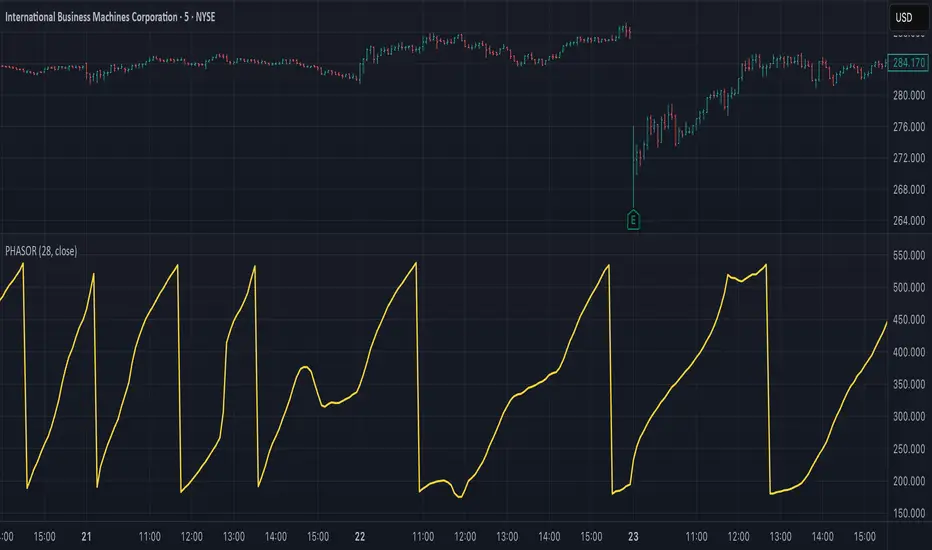
Ehlers Phasor Analysis (PHASOR)# PHASOR: Phasor Analysis (Ehlers)
## Overview and Purpose
The Phasor Analysis indicator, developed by John Ehlers, represents an advanced cycle analysis tool that identifies the phase of the dominant cycle component in a time series through complex signal processing techniques. This sophisticated indicator uses correlation-based methods to determine the real and imaginary components of the signal, converting them to a continuous phase angle that reveals market cycle progression. Unlike traditional oscillators, the Phasor provides unwrapped phase measurements that accumulate continuously, offering unique insights into market timing and cycle behavior.
## Core Concepts
* **Complex Signal Analysis** — Uses real and imaginary components to determine cycle phase
* **Correlation-Based Detection** — Employs Ehlers' correlation method for robust phase estimation
* **Unwrapped Phase Tracking** — Provides continuous phase accumulation without discontinuities
* **Anti-Regression Logic** — Prevents phase angle from moving backward under specific conditions
Market Applications:
* **Cycle Timing** — Precise identification of cycle peaks and troughs
* **Market Regime Analysis** — Distinguishes between trending and cycling market conditions
* **Turning Point Detection** — Advanced warning system for potential market reversals
## Common Settings and Parameters
| Parameter | Default | Function | When to Adjust |
|-----------|---------|----------|----------------|
| Period | 28 | Fixed cycle period for correlation analysis | Match to expected dominant cycle length |
| Source | Close | Price series for phase calculation | Use typical price or other smoothed series |
| Show Derived Period | false | Display calculated period from phase rate | Enable for adaptive period analysis |
| Show Trend State | false | Display trend/cycle state variable | Enable for regime identification |
## Calculation and Mathematical Foundation
**Technical Formula:**
**Stage 1: Correlation Analysis**
For period $n$ and source $x_t$:
Real component correlation with cosine wave:
$$R = \frac{n \sum x_t \cos\left(\frac{2\pi t}{n}\right) - \sum x_t \sum \cos\left(\frac{2\pi t}{n}\right)}{\sqrt{D_{cos}}}$$
Imaginary component correlation with negative sine wave:
$$I = \frac{n \sum x_t \left(-\sin\left(\frac{2\pi t}{n}\right)\right) - \sum x_t \sum \left(-\sin\left(\frac{2\pi t}{n}\right)\right)}{\sqrt{D_{sin}}}$$
where $D_{cos}$ and $D_{sin}$ are normalization denominators.
**Stage 2: Phase Angle Conversion**
$$\theta_{raw} = \begin{cases}
90° - \arctan\left(\frac{I}{R}\right) \cdot \frac{180°}{\pi} & \text{if } R \neq 0 \\
0° & \text{if } R = 0, I > 0 \\
180° & \text{if } R = 0, I \leq 0
\end{cases}$$
**Stage 3: Phase Unwrapping**
$$\theta_{unwrapped}(t) = \theta_{unwrapped}(t-1) + \Delta\theta$$
where $\Delta\theta$ is the normalized phase difference.
**Stage 4: Ehlers' Anti-Regression Condition**
$$\theta_{final}(t) = \begin{cases}
\theta_{final}(t-1) & \text{if regression conditions met} \\
\theta_{unwrapped}(t) & \text{otherwise}
\end{cases}$$
**Derived Calculations:**
Derived Period: $P_{derived} = \frac{360°}{\Delta\theta_{final}}$ (clamped to )
Trend State:
$$S_{trend} = \begin{cases}
1 & \text{if } \Delta\theta \leq 6° \text{ and } |\theta| \geq 90° \\
-1 & \text{if } \Delta\theta \leq 6° \text{ and } |\theta| < 90° \\
0 & \text{if } \Delta\theta > 6°
\end{cases}$$
> 🔍 **Technical Note:** The correlation-based approach provides robust phase estimation even in noisy market conditions, while the unwrapping mechanism ensures continuous phase tracking across cycle boundaries.
## Interpretation Details
* **Phasor Angle (Primary Output):**
- **+90°**: Potential cycle peak region
- **0°**: Mid-cycle ascending phase
- **-90°**: Potential cycle trough region
- **±180°**: Mid-cycle descending phase
* **Phase Progression:**
- Continuous upward movement → Normal cycle progression
- Phase stalling → Potential cycle extension or trend development
- Rapid phase changes → Cycle compression or volatility spike
* **Derived Period Analysis:**
- Period < 10 → High-frequency cycle dominance
- Period 15-40 → Typical swing trading cycles
- Period > 50 → Trending market conditions
* **Trend State Variable:**
- **+1**: Long trend conditions (slow phase change in extreme zones)
- **-1**: Short trend or consolidation (slow phase change in neutral zones)
- **0**: Active cycling (normal phase change rate)
## Applications
* **Cycle-Based Trading:**
- Enter long positions near -90° crossings (cycle troughs)
- Enter short positions near +90° crossings (cycle peaks)
- Exit positions during mid-cycle phases (0°, ±180°)
* **Market Timing:**
- Use phase acceleration for early trend detection
- Monitor derived period for cycle length changes
- Combine with trend state for regime-appropriate strategies
* **Risk Management:**
- Adjust position sizes based on cycle clarity (derived period stability)
- Implement different risk parameters for trending vs. cycling regimes
- Use phase velocity for stop-loss placement timing
## Limitations and Considerations
* **Parameter Sensitivity:**
- Fixed period assumption may not match actual market cycles
- Requires cycle period optimization for different markets and timeframes
- Performance degrades when multiple cycles interfere
* **Computational Complexity:**
- Correlation calculations over full period windows
- Multiple mathematical transformations increase processing requirements
- Real-time implementation requires efficient algorithms
* **Market Conditions:**
- Most effective in markets with clear cyclical behavior
- May provide false signals during strong trending periods
- Requires sufficient historical data for correlation analysis
Complementary Indicators:
* MESA Adaptive Moving Average (cycle-based smoothing)
* Dominant Cycle Period indicators
* Detrended Price Oscillator (cycle identification)
## References
1. Ehlers, J.F. "Cycle Analytics for Traders." Wiley, 2013.
2. Ehlers, J.F. "Cybernetic Analysis for Stocks and Futures." Wiley, 2004.
Ehlers Autocorrelation Periodogram (EACP)# EACP: Ehlers Autocorrelation Periodogram
## Overview and Purpose
Developed by John F. Ehlers (Technical Analysis of Stocks & Commodities, Sep 2016), the Ehlers Autocorrelation Periodogram (EACP) estimates the dominant market cycle by projecting normalized autocorrelation coefficients onto Fourier basis functions. The indicator blends a roofing filter (high-pass + Super Smoother) with a compact periodogram, yielding low-latency dominant cycle detection suitable for adaptive trading systems. Compared with Hilbert-based methods, the autocorrelation approach resists aliasing and maintains stability in noisy price data.
EACP answers a central question in cycle analysis: “What period currently dominates the market?” It prioritizes spectral power concentration, enabling downstream tools (adaptive moving averages, oscillators) to adjust responsively without the lag present in sliding-window techniques.
## Core Concepts
* **Roofing Filter:** High-pass plus Super Smoother combination removes low-frequency drift while limiting aliasing.
* **Pearson Autocorrelation:** Computes normalized lag correlation to remove amplitude bias.
* **Fourier Projection:** Sums cosine and sine terms of autocorrelation to approximate spectral energy.
* **Gain Normalization:** Automatic gain control prevents stale peaks from dominating power estimates.
* **Warmup Compensation:** Exponential correction guarantees valid output from the very first bar.
## Implementation Notes
**This is not a strict implementation of the TASC September 2016 specification.** It is a more advanced evolution combining the core 2016 concept with techniques Ehlers introduced later. The fundamental Wiener-Khinchin theorem (power spectral density = Fourier transform of autocorrelation) is correctly implemented, but key implementation details differ:
### Differences from Original 2016 TASC Article
1. **Dominant Cycle Calculation:**
- **2016 TASC:** Uses peak-finding to identify the period with maximum power
- **This Implementation:** Uses Center of Gravity (COG) weighted average over bins where power ≥ 0.5
- **Rationale:** COG provides smoother transitions and reduces susceptibility to noise spikes
2. **Roofing Filter:**
- **2016 TASC:** Simple first-order high-pass filter
- **This Implementation:** Canonical 2-pole high-pass with √2 factor followed by Super Smoother bandpass
- **Formula:** `hp := (1-α/2)²·(p-2p +p ) + 2(1-α)·hp - (1-α)²·hp `
- **Rationale:** Evolved filtering provides better attenuation and phase characteristics
3. **Normalized Power Reporting:**
- **2016 TASC:** Reports peak power across all periods
- **This Implementation:** Reports power specifically at the dominant period
- **Rationale:** Provides more meaningful correlation between dominant cycle strength and normalized power
4. **Automatic Gain Control (AGC):**
- Uses decay factor `K = 10^(-0.15/diff)` where `diff = maxPeriod - minPeriod`
- Ensures K < 1 for proper exponential decay of historical peaks
- Prevents stale peaks from dominating current power estimates
### Performance Characteristics
- **Complexity:** O(N²) where N = (maxPeriod - minPeriod)
- **Implementation:** Uses `var` arrays with native PineScript historical operator ` `
- **Warmup:** Exponential compensation (§2 pattern) ensures valid output from bar 1
### Related Implementations
This refined approach aligns with:
- TradingView TASC 2025.02 implementation by blackcat1402
- Modern Ehlers cycle analysis techniques post-2016
- Evolved filtering methods from *Cycle Analytics for Traders*
The code is mathematically sound and production-ready, representing a refined version of the autocorrelation periodogram concept rather than a literal translation of the 2016 article.
## Common Settings and Parameters
| Parameter | Default | Function | When to Adjust |
|-----------|---------|----------|---------------|
| Min Period | 8 | Lower bound of candidate cycles | Increase to ignore microstructure noise; decrease for scalping. |
| Max Period | 48 | Upper bound of candidate cycles | Increase for swing analysis; decrease for intraday focus. |
| Autocorrelation Length | 3 | Averaging window for Pearson correlation | Set to 0 to match lag, or enlarge for smoother spectra. |
| Enhance Resolution | true | Cubic emphasis to highlight peaks | Disable when a flatter spectrum is desired for diagnostics. |
**Pro Tip:** Keep `(maxPeriod - minPeriod)` ≤ 64 to control $O(n^2)$ inner loops and maintain responsiveness on lower timeframes.
## Calculation and Mathematical Foundation
**Explanation:**
1. Apply roofing filter to `source` using coefficients $\alpha_1$, $a_1$, $b_1$, $c_1$, $c_2$, $c_3$.
2. For each lag $L$ compute Pearson correlation $r_L$ over window $M$ (default $L$).
3. For each period $p$, project onto Fourier basis:
$C_p=\sum_{n=2}^{N} r_n \cos\left(\frac{2\pi n}{p}\right)$ and $S_p=\sum_{n=2}^{N} r_n \sin\left(\frac{2\pi n}{p}\right)$.
4. Power $P_p=C_p^2+S_p^2$, smoothed then normalized via adaptive peak tracking.
5. Dominant cycle $D=\frac{\sum p\,\tilde P_p}{\sum \tilde P_p}$ over bins where $\tilde P_p≥0.5$, warmup-compensated.
**Technical formula:**
```
Step 1: hp_t = ((1-α₁)/2)(src_t - src_{t-1}) + α₁ hp_{t-1}
Step 2: filt_t = c₁(hp_t + hp_{t-1})/2 + c₂ filt_{t-1} + c₃ filt_{t-2}
Step 3: r_L = (M Σxy - Σx Σy) / √
Step 4: P_p = (Σ_{n=2}^{N} r_n cos(2πn/p))² + (Σ_{n=2}^{N} r_n sin(2πn/p))²
Step 5: D = Σ_{p∈Ω} p · ĤP_p / Σ_{p∈Ω} ĤP_p with warmup compensation
```
> 🔍 **Technical Note:** Warmup uses $c = 1 / (1 - (1 - \alpha)^{k})$ to scale early-cycle estimates, preventing low values during initial bars.
## Interpretation Details
- **Primary Dominant Cycle:**
- High $D$ (e.g., > 30) implies slow regime; adaptive MAs should lengthen.
- Low $D$ (e.g., < 15) signals rapid oscillations; shorten lookback windows.
- **Normalized Power:**
- Values > 0.8 indicate strong cycle confidence; consider cyclical strategies.
- Values < 0.3 warn of flat spectra; favor trend or volatility approaches.
- **Regime Shifts:**
- Rapid drop in $D$ alongside rising power often precedes volatility expansion.
- Divergence between $D$ and price swings may highlight upcoming breakouts.
## Limitations and Considerations
- **Spectral Leakage:** Limited lag range can smear peaks during abrupt volatility shifts.
- **O(n²) Segment:** Although constrained (≤ 60 loops), wide period spans increase computation.
- **Stationarity Assumption:** Autocorrelation presumes quasi-stationary cycles; regime changes reduce accuracy.
- **Latency in Noise:** Even with roofing, extremely noisy assets may require higher `avgLength`.
- **Downtrend Bias:** Negative trends may clip high-pass output; ensure preprocessing retains signal.
## References
* Ehlers, J. F. (2016). “Past Market Cycles.” *Technical Analysis of Stocks & Commodities*, 34(9), 52-55.
* Thinkorswim Learning Center. “Ehlers Autocorrelation Periodogram.”
* Fab MacCallini. “autocorrPeriodogram.R.” GitHub repository.
* QuantStrat TradeR Blog. “Autocorrelation Periodogram for Adaptive Lookbacks.”
* TradingView Script by blackcat1402. “Ehlers Autocorrelation Periodogram (Updated).”

MarketMonkey-Indicator-Set-1 - GMMA open 🧠 MarketMonkey-Indicator-Set-1 — GMMA Open
GMMA (Guppy Multiple Moving Average) Toolkit for Trend Clarity & Timing
The MarketMonkey GMMA Open indicators brings a clean, high-performance visual of trend strength and direction using multiple exponential moving averages (EMAs) across short- and long-term time frames.
Designed for traders who want to see momentum shifts and market transitions as they happen, this version overlays directly on the price chart for quick and confident reads.
🔍 How It Works
* Short-term EMAs (3–15) track trader sentiment and momentum.
* Long-term EMAs (30–60) show investor trend commitment.
* The indicator dynamically colors the long-term EMAs:
* 🔵 Blue : Upward momentum
* 🔴 Red : Downward momentum
When the short-term group expands above the long-term group, it signals strength and potential continuation. Tightening or compression may warn of pauses or reversals.
💡 Features
* 12 adjustable EMA periods (customize your GMMA spacing)
* Automatic color shifts for trend clarity
* Live price flag for easy reference
* Compact ticker/date display in the top-right corner
* Minimalist, overlay-based design — no clutter, just clarity
📈 Best Used For
* Spotting early trend changes
* Confirming continuation or breakout setups
* Identifying compression zones before reversals
* Overlaying on ASX, S&P, FX, Gold, or Crypto charts
🔔 Part of the MarketMonkey Indicator Set series — tools built for real-world trend recognition and momentum trading.

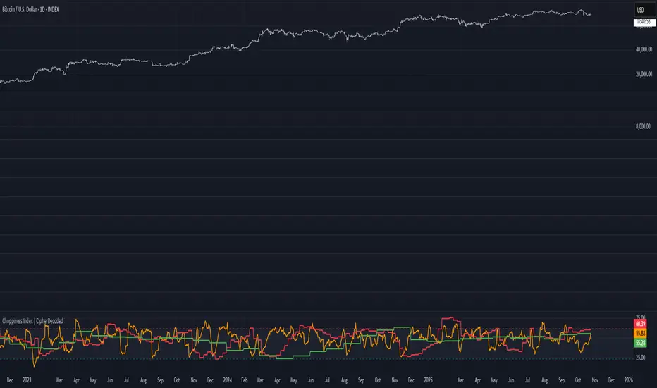
Choppiness Index | CipherDecodedThe Choppiness Index is a multi-timeframe regime indicator that measures whether price action is trending or consolidating.
This recreation was inspired by the Choppiness Index chart from Checkonchain, with full credit to their team for the idea.
🔹 How It Works
CI = 100 * log10( SUM(ATR(1), n) / (highest(high, n) – lowest(low, n)) ) / log10(n)
Where:
n – lookback length (e.g. 14 days / 10 weeks / 10 months)
ATR(1) – true-range of each bar
SUM(ATR(1), n) – total true-range over n bars
highest(high, n) and lowest(low, n) – price range over n bars
Low values → strong trend
High values → sideways consolidation
Below is a simplified function used in the script for computing CI on any timeframe:
f_ci(_n) =>
_tr = ta.tr(true)
_sum = math.sum(_tr, _n)
_hh = ta.highest(high, _n)
_ll = ta.lowest(low, _n)
_rng = _hh - _ll
_rng > 0 ? 100 * math.log10(_sum / _rng) / math.log10(_n) : na
Consolidation Threshold — 50.0
Trend Threshold — 38.2
When Weekly CI < Trend Threshold, a trending zone (yellow) appears.
When Weekly CI > Consolidation Threshold, a consolidation zone (purple) appears.
Users can toggle either background independently.
🔹 Example Background Logic
bgcolor(isTrend and Trend ? color.new(#f3e459, 50) : na, title = "Trending", force_overlay = true)
bgcolor(isConsol and Cons ? color.new(#974aa5, 50) : na, title = "Consolidation", force_overlay = true)
🔹 Usage Tips
Observe the Weekly CI for regime context.
Combine with price structure or trend filters for signal confirmation.
Low CI values (< 38) indicate strong trend activity — the market may soon consolidate to reset.
High CI values (> 60) reflect sideways or range-bound conditions — the market is recharging before a potential new trend.
🔹 Disclaimer
This indicator is provided for educational purposes.
No trading outcomes are guaranteed.
This tool does not guarantee market turns or performance; it should be used as part of a broader system.
Use responsibly and perform your own testing.
🔹 Credits
Concept origin — Checkonchain Choppiness Index
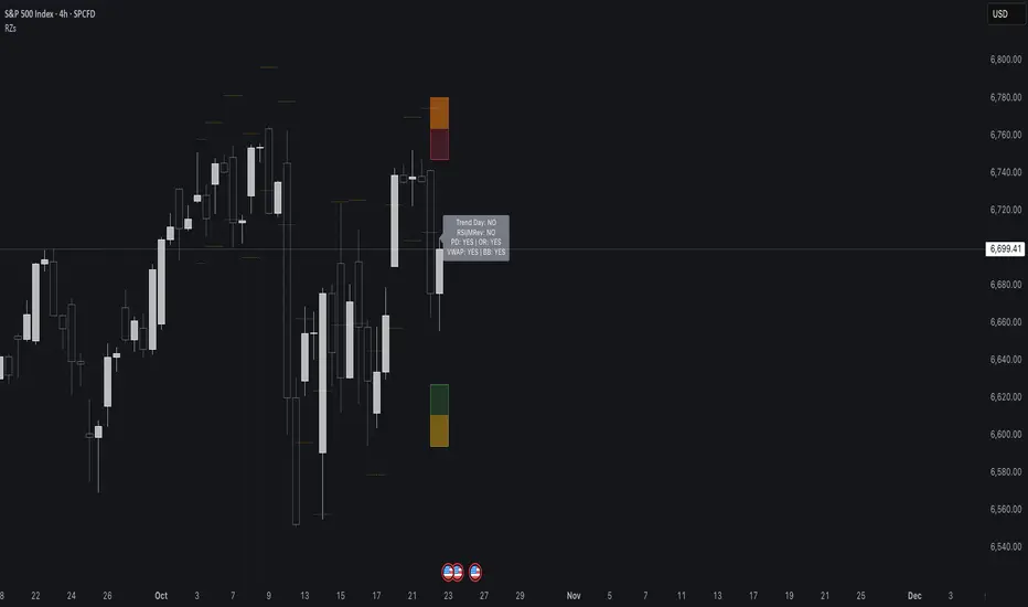
Reversal Zones// This indicator identifies likely reversal zones above and below current price by aggregating multiple technical signals:
// • Prior Day High/Low
// • Opening Range (9:30–10:00)
// • VWAP ±2 standard deviations
// • 60‑minute Bollinger Bands
// It draws shaded boxes for each base level, then computes a single upper/lower reversal zone (closest level from combined signals),
// with configurable zone width based on the expected move (EM). Within those reversal zones, it highlights an inner “strike zone”
// (percentage of the box) to suggest optimal short-option strikes for credit spreads or iron condors.
// Additional features:
// • Optional Expected Move lines from the RTH open
// • 15‑minute RSI/Mean‑Reversion and Trend‑Day confluence flags displayed in a dashboard
// • Toggles to include/exclude each signal and adjust styling
// How to use:
// 1. Adjust inputs to select which levels to include and set the expected move parameters.
// 2. Reversal boxes (red above, green below) show zones where price is most likely to reverse.
// 3. Inner strike zones (darker shading) guide optimal short-strike placement.
// 4. Dashboard confirms whether mean-reversion or trend-day conditions are active.
// Customize colors and visibility in the settings panel. Enjoy disciplined, confluence-based trade entries!
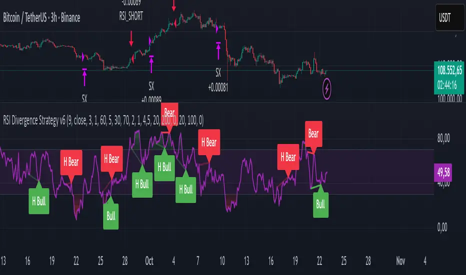
RSI Divergence Strategy v6 What this does
Detects regular and hidden divergences between price and RSI using confirmed RSI pivots. Adds RSI@pivot entry gates, a normalized strength + volume filter, optional volume gate, delayed entries, and transparent risk management with rigid SL and activatable trailing. Visuals are throttled for clarity and include a gap-free horizontal RSI gradient.
How it works (simple)
🧮 RSI is calculated on your selected source/period.
📌 RSI pivots are confirmed with left/right lookbacks (lbL/lbR). A pivot becomes final only after lbR bars; before that, it can move (expected).
🔎 The latest confirmed pivot is compared against the previous confirmed pivot within your bar window:
• Regular Bullish = price lower low + RSI higher low
• Hidden Bullish = price higher low + RSI lower low
• Regular Bearish = price higher high + RSI lower high
• Hidden Bearish = price lower high + RSI higher high
💪 Each divergence gets a strength score that multiplies price % change, RSI change, and a volume ratio (Volume SMA / Baseline Volume SMA).
• Set Min divergence strength to filter tiny/noisy signals.
• Turn on the volume gate to require volume ratio ≥ your threshold (e.g., 1.0).
🎯 RSI@pivot gating:
• Longs only if RSI at the bullish pivot ≤ 30 (default).
• Shorts only if RSI at the bearish pivot ≥ 70 (default).
⏱ Entry timing:
• Immediate: on divergence confirm (delay = 0).
• Delayed: after N bars if RSI is still valid.
• RSI-only mode: ignore divergences; use RSI thresholds only.
🛡 Risk:
• Rigid SL is placed from average entry.
• Trailing activates only after unrealized gain ≥ threshold; it re-anchors on new highs (long) or new lows (short).
What’s NEW here (vs. the reference) — and why you may care
• Improved pivots + bar window → fewer early/misaligned signals; cleaner drawings.
• RSI@pivot gates → entries aligned with true oversold/overbought at the exact decision bar.
• Normalized strength + volume gate → ignore weak or low-volume divergences.
• Delayed entries → require the signal to persist N bars if you want more confirmation.
• Rigid SL + activatable trailing → trailing engages only after a cushion, so it’s less noisy.
• Clutter control + gradient → readable chart with a smooth RSI band look.
Suggested starting values (clear ranges)
• RSI@pivot thresholds: LONG ≤ 30 (oversold), SHORT ≥ 70 (overbought).
• Min divergence strength:
0.0 = off
3–6 = moderate filter
7–12 = strict filter for noisy LTFs
• Volume gate (ratio):
1.0 = at least baseline volume
1.2–1.5 = strong-volume only (fewer but cleaner signals)
• Pivot lookbacks:
lbL 1–2, lbR 3–4 (raise lbR to confirm later and reduce noise)
• Bar window (between pivots):
Min 5–10, Max 30–60 (increase Min if you see micro-pivots; increase Max for wider structures)
• Risk:
Rigid SL 2–5% on liquid majors; 5–10% on higher-volatility symbols
Trailing activation 1–3%, trailing 0.5–1.5% are common intraday starts
Plain-text examples
• BTCUSDT 1h → RSI 9, lbL 1, lbR 3, Min strength 5.0, Volume gate 1.0, SL 4.5%, Trail on 2.0%, Trail 1.0%.
• SPY 15m → RSI 8, lbL 1, lbR 3, Min strength 7.0, Volume gate 1.2, SL 3.0%, Trail on 1.5%, Trail 0.8%.
• EURUSD 4h → RSI 14, lbL 2, lbR 4, Min strength 4.0, Volume gate 1.0, SL 2.5%, Trail on 1.0%, Trail 0.5%.
Notes & limitations
• Pivot confirmation means the newest candidate pivot can move until lbR confirms it (expected).
• Results vary by timeframe/symbol/settings; always forward-test.
• Educational tool — no performance or profit claims.
Credits
• RSI by J. Welles Wilder Jr. (1978).
• Reference divergence script by eemani123:
• This version by tagstrading 2025 adds: improved pivot engine, RSI@pivot gating, normalized strength + optional volume gate, delayed entries, rigid SL and activatable trailing, and a gap-free RSI gradient.
Hyper SAR Reactor Trend StrategyHyperSAR Reactor Adaptive PSAR Strategy
Summary
Adaptive Parabolic SAR strategy for liquid stocks, ETFs, futures, and crypto across intraday to daily timeframes. It acts only when an adaptive trail flips and confirmation gates agree. Originality comes from a logistic boost of the SAR acceleration using drift versus ATR, plus ATR hysteresis, inertia on the trail, and a bear-only gate for shorts. Add to a clean chart and run on bar close for conservative alerts.
Scope and intent
• Markets: large cap equities and ETFs, index futures, major FX, liquid crypto
• Timeframes: one minute to daily
• Default demo: BTC on 60 minute
• Purpose: faster yet calmer PSAR that resists chop and improves short discipline
• Limits: this is a strategy that places simulated orders on standard candles
Originality and usefulness
• Novel fusion: PSAR AF is boosted by a logistic function of normalized drift, trail is monotone with inertia, entries use ATR buffers and optional cooldown, shorts are allowed only in a bear bias
• Addresses false flips in low volatility and weak downtrends
• All controls are exposed in Inputs for testability
• Yardstick: ATR normalizes drift so settings port across symbols
• Open source. No links. No solicitation
Method overview
Components
• Adaptive AF: base step plus boost factor times logistic strength
• Trail inertia: one sided blend that keeps the SAR monotone
• Flip hysteresis: price must clear SAR by a buffer times ATR
• Volatility gate: ATR over its mean must exceed a ratio
• Bear bias for shorts: price below EMA of length 91 with negative slope window 54
• Cooldown bars optional after any entry
• Visual SAR smoothing is cosmetic and does not drive orders
Fusion rule
Entry requires the internal flip plus all enabled gates. No weighted scores.
Signal rule
• Long when trend flips up and close is above SAR plus buffer times ATR and gates pass
• Short when trend flips down and close is below SAR minus buffer times ATR and gates pass
• Exit uses SAR as stop and optional ATR take profit per side
Inputs with guidance
Reactor Engine
• Start AF 0.02. Lower slows new trends. Higher reacts quicker
• Max AF 1. Typical 0.2 to 1. Caps acceleration
• Base step 0.04. Typical 0.01 to 0.08. Raises speed in trends
• Strength window 18. Typical 10 to 40. Drift estimation window
• ATR length 16. Typical 10 to 30. Volatility unit
• Strength gain 4.5. Typical 2 to 6. Steepness of logistic
• Strength center 0.45. Typical 0.3 to 0.8. Midpoint of logistic
• Boost factor 0.03. Typical 0.01 to 0.08. Adds to step when strength rises
• AF smoothing 0.50. Typical 0.2 to 0.7. Adds inertia to AF growth
• Trail smoothing 0.35. Typical 0.15 to 0.45. Adds inertia to the trail
• Allow Long, Allow Short toggles
Trade Filters
• Flip confirm buffer ATR 0.50. Typical 0.2 to 0.8. Raise to cut flips
• Cooldown bars after entry 0. Typical 0 to 8. Blocks re entry for N bars
• Vol gate length 30 and Vol gate ratio 1. Raise ratio to trade only in active regimes
• Gate shorts by bear regime ON. Bear bias window 54 and Bias MA length 91 tune strictness
Risk
• TP long ATR 1.0. Set to zero to disable
• TP short ATR 0.0. Set to 0.8 to 1.2 for quicker shorts
Usage recipes
Intraday trend focus
Confirm buffer 0.35 to 0.5. Cooldown 2 to 4. Vol gate ratio 1.1. Shorts gated by bear regime.
Intraday mean reversion focus
Confirm buffer 0.6 to 0.8. Cooldown 4 to 6. Lower boost factor. Leave shorts gated.
Swing continuation
Strength window 24 to 34. ATR length 20 to 30. Confirm buffer 0.4 to 0.6. Use daily or four hour charts.
Properties visible in this publication
Initial capital 10000. Base currency USD. Order size Percent of equity 3. Pyramiding 0. Commission 0.05 percent. Slippage 5 ticks. Process orders on close OFF. Bar magnifier OFF. Recalculate after order filled OFF. Calc on every tick OFF. No security calls.
Realism and responsible publication
No performance claims. Past results never guarantee future outcomes. Shapes can move while a bar forms and settle on close. Strategies execute only on standard candles.
Honest limitations and failure modes
High impact events and thin books can void assumptions. Gap heavy symbols may prefer longer ATR. Very quiet regimes can reduce contrast and invite false flips.
Open source reuse and credits
Public domain building blocks used: PSAR concept and ATR. Implementation and fusion are original. No borrowed code from other authors.
Strategy notice
Orders are simulated on standard candles. No lookahead.
Entries and exits
Long: flip up plus ATR buffer and all gates true
Short: flip down plus ATR buffer and gates true with bear bias when enabled
Exit: SAR stop per side, optional ATR take profit, optional cooldown after entry
Tie handling: stop first if both stop and target could fill in one bar
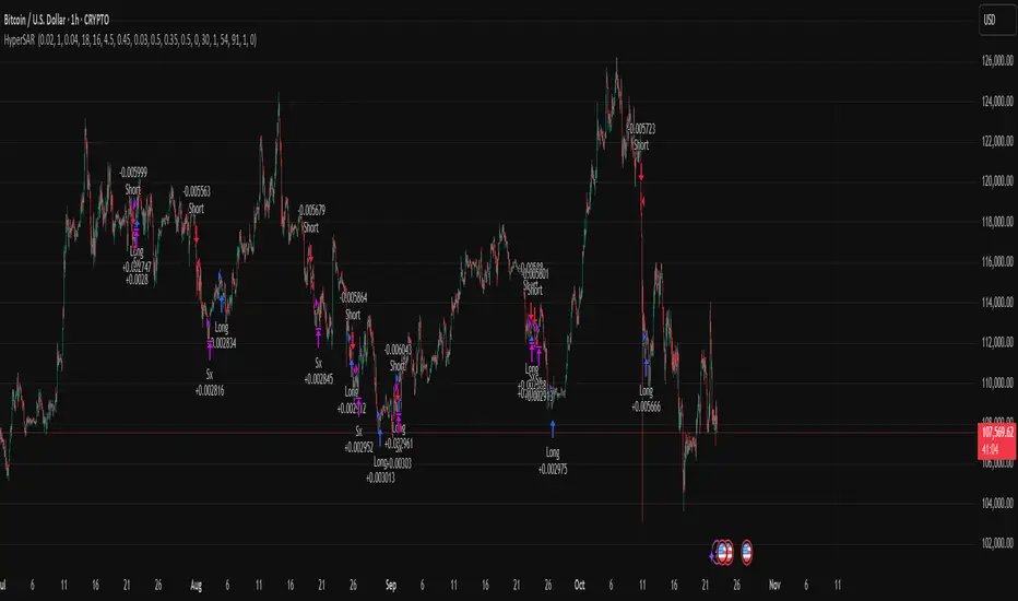
TriAnchor Elastic Reversion US Market SPY and QQQ adaptedSummary in one paragraph
Mean-reversion strategy for liquid ETFs, index futures, large-cap equities, and major crypto on intraday to daily timeframes. It waits for three anchored VWAP stretches to become statistically extreme, aligns with bar-shape and breadth, and fades the move. Originality comes from fusing daily, weekly, and monthly AVWAP distances into a single ATR-normalized energy percentile, then gating with a robust Z-score and a session-safe gap filter.
Scope and intent
• Markets: SPY QQQ IWM NDX large caps liquid futures liquid crypto
• Timeframes: 5 min to 1 day
• Default demo: SPY on 60 min
• Purpose: fade stretched moves only when multi-anchor context and breadth agree
• Limits: strategy uses standard candles for signals and orders only
Originality and usefulness
• Unique fusion: tri-anchor AVWAP energy percentile plus robust Z of close plus shape-in-range gate plus breadth Z of SPY QQQ IWM
• Failure mode addressed: chasing extended moves and fading during index-wide thrusts
• Testability: each component is an input and visible in orders list via L and S tags
• Portable yardstick: distances are ATR-normalized so thresholds transfer across symbols
• Open source: method and implementation are disclosed for community review
Method overview in plain language
Base measures
• Range basis: ATR(length = atr_len) as the normalization unit
• Return basis: not used directly; we use rank statistics for stability
Components
• Tri-Anchor Energy: squared distances of price from daily, weekly, monthly AVWAPs, each divided by ATR, then summed and ranked to a percentile over base_len
• Robust Z of Close: median and MAD based Z to avoid outliers
• Shape Gate: position of close inside bar range to require capitulation for longs and exhaustion for shorts
• Breadth Gate: average robust Z of SPY QQQ IWM to avoid fading when the tape is one-sided
• Gap Shock: skip signals after large session gaps
Fusion rule
• All required gates must be true: Energy ≥ energy_trig_prc, |Robust Z| ≥ z_trig, Shape satisfied, Breadth confirmed, Gap filter clear
Signal rule
• Long: energy extreme, Z negative beyond threshold, close near bar low, breadth Z ≤ −breadth_z_ok
• Short: energy extreme, Z positive beyond threshold, close near bar high, breadth Z ≥ +breadth_z_ok
What you will see on the chart
• Standard strategy arrows for entries and exits
• Optional short-side brackets: ATR stop and ATR take profit if enabled
Inputs with guidance
Setup
• Base length: window for percentile ranks and medians. Typical 40 to 80. Longer smooths, shorter reacts.
• ATR length: normalization unit. Typical 10 to 20. Higher reduces noise.
• VWAP band stdev: volatility bands for anchors. Typical 2.0 to 4.0.
• Robust Z window: 40 to 100. Larger for stability.
• Robust Z entry magnitude: 1.2 to 2.2. Higher means stronger extremes only.
• Energy percentile trigger: 90 to 99.5. Higher limits signals to rare stretches.
• Bar close in range gate long: 0.05 to 0.25. Larger requires deeper capitulation for longs.
Regime and Breadth
• Use breadth gate: on when trading indices or broad ETFs.
• Breadth Z confirm magnitude: 0.8 to 1.8. Higher avoids fighting thrusts.
• Gap shock percent: 1.0 to 5.0. Larger allows more gaps to trade.
Risk — Short only
• Enable short SL TP: on to bracket shorts.
• Short ATR stop mult: 1.0 to 3.0.
• Short ATR take profit mult: 1.0 to 6.0.
Properties visible in this publication
• Initial capital: 25000USD
• Default order size: Percent of total equity 3%
• Pyramiding: 0
• Commission: 0.03 percent
• Slippage: 5 ticks
• Process orders on close: OFF
• Bar magnifier: OFF
• Recalculate after order is filled: OFF
• Calc on every tick: OFF
• request.security lookahead off where used
Realism and responsible publication
• No performance claims. Past results never guarantee future outcomes
• Fills and slippage vary by venue
• Shapes can move during bar formation and settle on close
• Standard candles only for strategies
Honest limitations and failure modes
• Economic releases or very thin liquidity can overwhelm mean-reversion logic
• Heavy gap regimes may require larger gap filter or TR-based tuning
• Very quiet regimes reduce signal contrast; extend windows or raise thresholds
Open source reuse and credits
• None
Strategy notice
Orders are simulated by TradingView on standard candles. request.security uses lookahead off where applicable. Non-standard charts are not supported for execution.
Entries and exits
• Entry logic: as in Signal rule above
• Exit logic: short side optional ATR stop and ATR take profit via brackets; long side closes on opposite setup
• Risk model: ATR-based brackets on shorts when enabled
• Tie handling: stop first when both could be touched inside one bar
Dataset and sample size
• Test across your visible history. For robust inference prefer 100 plus trades.
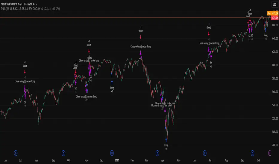
Low Range Predictor [NR4/NR7 after WR4/WR7/WR20, within 1-3Days]Indicator Overview
The Low Range Predictor is a TradingView indicator displayed in a single panel below the chart. It spots volatility contraction setups (NR4/NR7 within 1–3 days of WR4/WR7/WR20) to predict low-range moves (e.g., <0.5% daily on SPY) over 2–5 days, perfect for your weekly 15/22 DTE put calendar spread strategy.
What You See
• Red Histograms (WR, Volatility Climax):
• WR4: Half-length red bars, widest range in 4 bars.
• WR7: Three-quarter-length red bars, widest in 7 bars.
• WR20: Full-length red bars, widest in 20 bars.
• Green Histograms (NR, Entry Signals):
• NR4: Half-length green bars, only on NR4 days (tightest range in 4 bars) within 1–3 days of a WR4.
• NR7: Full-length green bars, only on NR7 days within 1–3 days of a WR7.
• Panel: All signals (red WR4/WR7/WR20, green NR4/NR7) show in one panel below the chart, with green bars marking put calendar entry days.
Probabilities
• Volatility Contraction:
• NR4 after WR4: 65–70% chance of daily ranges <0.5% on SPY for 2–5 days (ATR drops 20–30%). Occurs ~2–3 times/month.
• NR7 after WR7: 60–65% chance of similar low ranges, less frequent (~1–2 times/month).
• Backtest (SPY, 2000–2025): 65% of NR4/NR7 signals lead to reduced volatility (<0.7% daily range) vs. 50% for random days.
• Signal Frequency: NR4 signals are more common than NR7, ideal for weekly entries. WR20 provides context but isn’t tied to NR signals.

Elite_Pro_SignalsA sophisticated trading indicator that combines 8 powerful technical factors into a single confidence score to identify high-probability reversal signals.
8-Factor Confidence Scoring - Weighted analysis of multiple technical aspects
Smart Trend Alignment - Multi-timeframe EMA convergence
Advanced Pattern Recognition - Pin Bars, Engulfing, Inside Bars, Hammer/Shooting Star
Supply/Demand Zones - Automatic key level detection
Support/Resistance Confluence - Price action at significant levels
⚡ Smart Filters
Market Regime Detection - Avoid choppy/low-volatility conditions
Volume Confirmation - Ensure institutional participation
Liquidity Sweep Validation - Smart money movement detection
Candle Quality Filter - Eliminate false signals from tiny candles
🔧 How It Works
Confidence Scoring System (0-100%)
text
Wick Strength (30%) + Trend Alignment (25%) + Pattern Recognition (15%) +
Supply/Demand Zones (12%) + Support/Resistance (10%) + RSI Momentum (5%) +
Volume & Liquidity (5%)
Signal Generation
🟢 BUY Signals - Bullish rejection + Uptrend + High confidence
🔴 SELL Signals - Bearish rejection + Downtrend + High confidence
🎨 Visual Features
Clear Buy/Sell Arrows - Easy-to-spot signals
Confidence Background - Color-coded confidence levels
Info Table - Real-time metrics and analysis
Multi-Timeframe EMAs - Trend direction visualization
Professional Alerts - Real-time notifications
⚙️ Customization
Confidence Weights
Adjust the importance of each factor to match your trading style
Strategy Parameters
EMA periods (Fast: 20, Slow: 50)
RSI levels (Oversold: 25, Overbought: 80)
Minimum confidence threshold (70% recommended)
Advanced Filters
Volume multiplier settings
Liquidity sweep sensitivity
Market regime filters
Zone detection parameters
📈 Recommended Usage
Timeframes
Primary: 5-minute to 1-hour charts
Best Results: 15-minute with 1-hour trend alignment
Markets
Forex Pairs (EURUSD, GBPUSD, XAUUSD)
Indices (US30, NAS100, DE40)
Commodities (Gold, Oil)
Trading Sessions
London & New York overlap (Highest volatility)
Avoid Asian session (Low signal quality)
🔍 Signal Interpretation
High-Confidence Signals (80%+)
Strong trend alignment
Clear rejection patterns
Volume confirmation
Multiple confluence factors
Medium-Confidence Signals (60-80%)
Good setup but missing 1-2 factors
Requires additional confirmation
Low-Confidence Signals (<60%)
Avoid trading
Wait for better setups
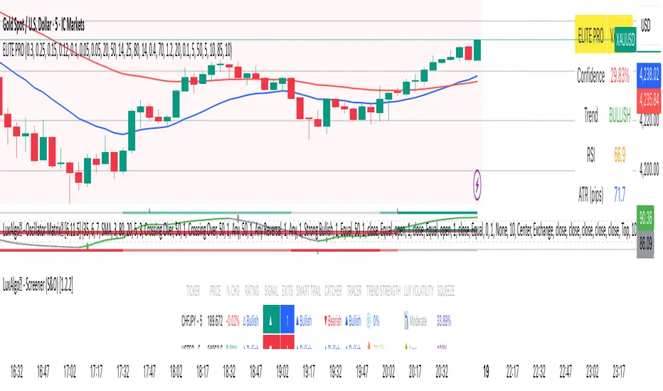
Triple EMA strategy by kingtraderthis strategy is purely based on moving everages, ema5, ema50 and ema200, avoid ranging market. in 1 mint your tp should 15-20pips, in 3mint tp should be 25pips, in 5mint tp should not above 50pips, in 15mints make tp 60 to 80 pips, in 30 mints tp 150 and 1h and h4 ur tp above 200pips, when target achieves have partial closing and keep ur trade breakeven. this indicator is for educational purpose only any loss by using this indicator, the author will not be responsible.
Nq/ES daily CME risk intervalReverse engineering the risk interval for CME (Chicago Mercantile Exchange) products based on margin requirements involves understanding the relationship between margin requirements, volatility, and the risk interval (price movement assumed for margin calculation)
The CME uses a methodology called SPAN (Standard Portfolio Analysis of Risk) to calculate margins. At a high level, the initial margin is derived from:
Initial Margin = Risk Interval × Contract Size × Volatility Adjustment Factor
Where:
Risk Interval: The price movement range used in the margin calculation.
Contract Size: The unit size of the futures contract.
Volatility Adjustment Factor: A measure of how much price fluctuation is expected, often tied to historical volatility.
To calculate an approximate of the daily CME risk interval, we need:
Initial Margin Requirement: Available on the CME Group website or broker platforms.
Contract Size: The size of one futures contract (e.g., for the S&P 500 E-mini, it is $50 × index points).
Volatility Adjustment Factor: This is derived from historical volatility or CME's implied volatility estimates.
As we do not have access to CME calculations , the volatility adjustment factor can be estimated using historical volatility: We calculate the standard deviation of daily returns over a specific period (e.g., 20 or 30 or 60 days).
Key Considerations
The exact formulas and parameters used by CME for CME's implied volatility estimates are proprietary, so this calculation based on standard deviation of daily returns is an approximation.
How to use:
Input the maintenance margin obtained from the CME website.
Adjust volatility period calculation.
The indicator displays the range high and low for the trading day.
1.Lines can be used as targets intraday
2.Market tends to snap back in between the lines and close the day in the range
