TQQQ Vibha Strategy – Auto Ranges + Rally Days1. Buy only after an intermediate bottom
A 20-day lowest low becomes the potential bottom.
2. Wait 3–4 days of higher highs & higher lows
higherSeq logic enforces that.
3. Avoid buying when too extended from the 200-day
Enforced with:
close <= ma200 * (1 + maxExtension) (default 10%)
4. Must close back above 200-day
Needed for “change of character”
5. Sell immediately if price breaks the Day-1 rally low (“line in the sand”)
Script sets lineInSand = bottom low
If price undercuts → close position immediately
6. Range-top rejection
Track touches of range top (highest high since bottom)
Three failures = sell (“3 strikes rule”)
Search in scripts for "200元+股票大盘"

Price Volume Heatmap [MHA Finverse]Price Volume Heatmap - Advanced Volume Profile Analysis
Unlock the power of institutional-level volume analysis with the Price Volume Heatmap indicator. This sophisticated tool visualizes market structure through volume distribution across price levels, helping you identify key support/resistance zones, high-probability reversal areas, and optimal entry/exit points.
🎯 What Makes This Indicator Unique?
Unlike traditional volume indicators that only show volume over time, this heatmap displays volume distribution across price levels , revealing where the most significant trading activity occurred. The gradient coloring system instantly highlights high-volume nodes (areas of strong interest) and low-volume nodes (potential breakout zones).
📊 Core Features
1. Dynamic Volume Heatmap
- Visualizes volume concentration across 250 customizable price levels
- Gradient color scheme from high volume (white) to low volume (teal/green)
- Adjustable brightness multiplier for enhanced contrast and clarity
- Real-time updates as market conditions evolve
2. Point of Control (POC)
- Automatically identifies the price level with the highest traded volume
- Acts as a magnetic price level where markets often return
- Critical for identifying fair value areas and potential reversal zones
- Customizable line style, width, and color
3. Flexible Lookback Settings
- Lookback Bars: Set any value from 1-5000 bars to control analysis depth
- Visible Range Mode: Analyze only what's currently visible on your chart
- Timeframe-Specific Settings: Different lookback periods for 1m, 5m, 15m, 30m, 1h, Daily, and Weekly charts
- Adapts to your trading style - scalping to position trading
4. Session Separation Analysis
- Tokyo Session: 00:00-09:00 UTC
- London Session: 07:00-16:00 UTC
- New York Session: 13:00-22:00 UTC
- Sydney Session: 21:00-06:00 UTC
- Daily Reset: Analyze each trading day independently
Session separation allows you to understand volume distribution specific to each major trading session, revealing institutional order flow patterns and session-specific support/resistance levels.
5. Profile Width Options
- Dynamic: Profile width adjusts based on lookback period
- Fixed Bars: Set a specific bar count for consistent profile width
- Extend Forward: Project the profile into future bars for planning trades
6. Smart Alerts
- POC crossover/crossunder alerts
- New session start notifications
- Never miss critical price action at high-volume nodes
📈 How to Use This Indicator Professionally
Understanding Market Structure:
High Volume Nodes (HVN):
- Appear as bright/white areas in the heatmap
- Represent price levels where significant trading occurred
- Act as strong support/resistance zones
- Markets often consolidate or bounce from these levels
- Trading Strategy: Look for entries when price tests HVN areas with confluence from other indicators
Low Volume Nodes (LVN):
- Appear as darker/teal areas in the heatmap
- Represent price levels with minimal trading activity
- Price tends to move quickly through these areas
- Often form "gaps" in the volume profile
- Trading Strategy: Expect rapid price movement through LVN zones; avoid placing stop losses here
Point of Control (POC):
- The single most important price level in your analysis window
- Represents the fairest price where maximum volume traded
- Price gravitates toward POC like a magnet
- Trading Strategy:
* When price is above POC: bullish bias, POC acts as support
* When price is below POC: bearish bias, POC acts as resistance
* POC breaks often lead to significant trend changes
Session-Based Analysis:
Use session separation to understand how different market participants trade:
Asian Session (Tokyo/Sydney):
- Typically lower volatility and range-bound
- Volume profiles often show tight, balanced distribution
- Use for identifying overnight ranges and gap fill zones
London Session:
- Highest volume session for forex pairs
- Often shows strong directional bias
- Look for breakouts from Asian ranges during London open
New York Session:
- Maximum participation when overlapping with London
- Institutional order flow most visible
- POC during NY session often becomes key level for following sessions
🎯 Practical Trading Applications
1. Identifying Support & Resistance:
High volume nodes from the heatmap are far more reliable than traditional swing highs/lows. When price approaches an HVN, expect reaction - either a bounce or a significant breakout if breached.
2. Trend Confirmation:
- Healthy uptrend: POC rising over time, HVN forming at higher levels
- Healthy downtrend: POC falling over time, HVN forming at lower levels
- Consolidation: POC relatively flat, volume balanced across range
3. Breakout Trading:
When price breaks through a Low Volume Node with momentum, it often continues to the next High Volume Node. Use LVN areas as measured move targets.
4. Reversal Zones:
Multiple HVN stacking on top of each other creates a "volume shelf" - an extremely strong support/resistance zone where reversals are highly probable.
5. Risk Management:
- Place stops beyond HVN areas (not within LVN zones)
- Size positions based on distance to nearest HVN
- Use POC as trailing stop level in trending markets
⚙️ Recommended Settings
For Day Trading (Scalping/Intraday):
- Lookback: 200-500 bars
- Rows: 200-250
- Enable session separation for your primary trading session
- Profile Width: Dynamic or Fixed Bars (30-50)
For Swing Trading:
- Lookback: 500-1000 bars
- Rows: 250
- Session separation: Daily Reset
- Profile Width: Dynamic
For Position Trading:
- Lookback: 1000-3000 bars
- Rows: 250
- Use timeframe-specific settings
- Profile Width: Extend Forward (20-50 bars)
💡 Pro Tips
1. Combine this indicator with price action analysis - volume confirms what price is telling you
2. Watch for POC convergence with other technical levels (fibonacci, pivot points, moving averages)
3. Volume at extremes (tops/bottoms of heatmap) often indicates exhaustion
4. Session POC from previous sessions often acts as magnet for current session
5. Increase brightness multiplier (1.5-2.5) for clearer visualization on busy charts
6. Use "Number of Sessions to Display" to analyze consistency of volume levels across multiple sessions
🎨 Customization
Fully customizable visual appearance:
- Gradient colors for volume visualization
- POC line thickness, color, and style
- Session line colors and visibility
- All settings organized in intuitive groups
⚠️ Disclaimer
This indicator is a technical analysis tool and should not be used as the sole basis for trading decisions. Always combine volume analysis with proper risk management, fundamental analysis, and other technical indicators. Past performance does not guarantee future results.
---
Support & Updates
Regular updates and improvements are made to enhance functionality. For questions, suggestions, or bug reports, please use the comments section below.
Happy Trading! 📊💹

VMDM - Volume, Momentum & Divergence Master [BullByte]VMDM - Volume, Momentum and Divergence Master
Educational Multi-Layer Market Structure Analysis System
Multi-factor divergence engine that scores RSI momentum, volume pressure, and institutional footprints into one non-repainting confluence rating (0-100).
WHAT THIS INDICATOR IS
VMDM is an educational indicator designed to teach traders how to recognize high-probability reversal and continuation patterns by analyzing four independent market dimensions simultaneously. Instead of relying on a single indicator that may produce frequent false signals, VMDM creates a confluence-based scoring system that weights multiple confirmation factors, helping you understand which setups have stronger technical backing and which are lower quality.
This is NOT a trading system or signal generator. It is a learning tool that visualizes complex market structure concepts in an accessible format for both coders and non-coders.
THE PROBLEM IT SOLVES
Most traders face these common challenges:
Challenge 1 - Indicator Overload: Running RSI, volume analysis, and divergence detection separately creates chart clutter and conflicting signals. You waste time cross-referencing multiple windows trying to determine if all factors align.
Challenge 2 - False Divergences: Standard divergence indicators trigger on every minor pivot, creating noise. Many divergences fail because they lack supporting evidence from volume or market structure.
Challenge 3 - Missed Context: A bullish RSI divergence means nothing if it occurs during weak volume or in the middle of strong distribution. Context determines quality.
Challenge 4 - Repainting Confusion: Many divergence scripts repaint, showing perfect historical signals that never actually triggered in real-time, leading to false confidence.
Challenge 5 - Institutional Pattern Recognition: Absorption zones, stop hunts, and exhaustion patterns are taught in trading education but difficult to identify systematically without manual analysis.
VMDM addresses all five challenges by combining complementary analytical layers into one transparent, non-repainting, confluence-weighted system with visual clarity.
WHY THIS SPECIFIC COMBINATION - MASHUP JUSTIFICATION
This indicator is NOT a random mashup of popular indicators. Each of the four layers serves a specific analytical purpose and together they create a complete market structure assessment framework.
THE FOUR ANALYTICAL LAYERS
LAYER 1 - RSI MOMENTUM DIVERGENCE (Trend Exhaustion Detection)
Purpose: Identifies when price momentum is weakening before price itself reverses.
Why RSI: The Relative Strength Index measures momentum on a bounded 0-100 scale, making divergence detection mathematically consistent across all assets and timeframes. Unlike raw price oscillators, RSI normalizes momentum regardless of volatility regime.
How It Contributes: Divergence between price pivots and RSI pivots reveals early momentum exhaustion. A lower price low with a higher RSI low (bullish regular divergence) signals sellers are losing strength even as price makes new lows. This is the PRIMARY signal generator in VMDM.
Limitation If Used Alone: RSI divergence by itself produces many false signals because momentum can remain weak during continued trends. It needs confirmation from volume and structural evidence.
LAYER 2 - VOLUME PRESSURE ANALYSIS (Buying vs Selling Intensity)
Purpose: Quantifies whether the current bar's volume reflects buying pressure or selling pressure based on where price closed within the bar's range.
Methodology: Instead of just measuring volume size, VMDM calculates WHERE in the bar range the close occurred. A close near the high on high volume indicates strong buying absorption. A close near the low indicates selling pressure. The calculation accounts for wick size (wicks reduce pressure quality) and uses percentile ranking over a lookback period to normalize pressure strength on a 0-100 scale.
Formula Concept:
Buy Pressure = Volume × (Close - Low) / (High - Low) × Wick Quality Factor
Sell Pressure = Volume × (High - Close) / (High - Low) × Wick Quality Factor
Net Pressure = Buy Pressure - Sell Pressure
Pressure Strength = Percentile Rank of Net Pressure over lookback period
Why Percentile Ranking: Absolute volume varies by asset and session. Percentile ranking makes 85th percentile pressure on low-volume crypto comparable to 85th percentile pressure on high-volume forex.
How It Contributes: When a bullish divergence occurs at a pivot low AND pressure strength is above 60 (strong buying), this adds 25 confluence points. It confirms that the divergence is occurring during actual accumulation, not just weak selling.
Limitation If Used Alone: Pressure analysis shows current bar intensity but cannot identify trend exhaustion or reversal timing. High buying pressure can exist during a strong uptrend with no reversal imminent.
LAYER 3 - BEHAVIORAL FOOTPRINT PATTERNS (Volume Anomaly Detection)
CRITICAL DISCLAIMER: The terms "institutional footprint," "absorption," "stop hunt," and "exhaustion" used in this indicator are EDUCATIONAL LABELS for specific price and volume behavioral patterns. These patterns are detected through technical analysis of publicly available price, volume, and bar structure data. This indicator does NOT have access to actual institutional order flow, market maker data, broker stop-loss locations, or any non-public data source. These pattern names are used because they are common terminology in trading education to describe these technical behaviors. The analysis is interpretive and based on observable price action, not privileged information.
Purpose: Detect volume anomalies and price patterns that historically correlate with potential reversal zones or trend continuation failure.
Pattern Type 1 - Absorption (Labeled as "ACCUMULATION" or "DISTRIBUTION")
Detection Criteria: Volume is more than 2x the moving average AND bar range is less than 50 percent of the average bar range.
Interpretation: High volume compressed into a tight range suggests large participants are absorbing supply (accumulation) or distribution (distribution) without allowing price to move significantly. This often precedes directional moves once absorption completes.
Visual: Colored box zone highlighting the absorption area.
Pattern Type 2 - Stop Hunt (Labeled as "BULL HUNT" or "BEAR HUNT")
Detection Criteria: Price penetrates a recent 10-bar high or low by a small margin (0.2 percent), then closes back inside the range on above-average volume (1.5x+).
Interpretation: Price briefly spikes beyond recent structure (likely triggering stop losses placed just beyond obvious levels) then reverses. This is a classic false breakout pattern often seen before reversals.
Visual: Label at the wick extreme showing hunt direction.
Pattern Type 3 - Exhaustion (Labeled as "SELL EXHAUST" or "BUY EXHAUST")
Detection Criteria: Lower wick is more than 2.5x the body size with volume above 1.8x average and RSI below 35 (sell exhaustion), OR upper wick more than 2.5x body size with volume above 1.8x average and RSI above 65 (buy exhaustion).
Interpretation: Large wicks with high volume and extreme RSI suggest aggressive buying or selling was met with equally aggressive rejection. This exhaustion often marks short-term extremes.
Visual: Label showing exhaustion type.
How These Contribute: When a divergence forms at a pivot AND one of these behavioral patterns is active, the confluence score increases by 20 points. This confirms the divergence is occurring during structural anomaly activity, not just normal price flow.
Limitation If Used Alone: These patterns can occur mid-trend and do not indicate direction without momentum context. Absorption in a strong uptrend may just be continuation accumulation.
LAYER 4 - CONFLUENCE SCORING MATRIX (Quality Weighting System)
Purpose: Translate all detected conditions into a single 0-100 quality score so you can objectively compare setups.
Scoring Breakdown:
Divergence Present: +30 points (primary signal)
Pressure Confirmation: +25 points (volume supports direction)
Behavioral Footprint Active: +20 points (structural anomaly present)
RSI Extreme: +15 points (RSI below 30 or above 70 at pivot)
Volume Spike: +10 points (current volume above 1.5x average)
Maximum Possible Score: 100 points
Why These Weights: The weights reflect reliability hierarchy based on backtesting observation. Divergence is the core signal (30 points), but without volume confirmation (25 points) many fail. Behavioral patterns add meaningful context (20 points). RSI extremes and volume spikes are secondary confirmations (15 and 10 points).
Quality Tiers:
90-100: TEXTBOOK (all factors aligned)
75-89: HIGH QUALITY (strong confluence)
60-74: VALID (meets minimum threshold)
Below 60: DEVELOPING (not displayed unless threshold lowered)
How It Contributes: The confluence score allows you to filter noise. You can set your minimum quality threshold in settings. Higher thresholds (75+) show fewer but higher-quality patterns. Lower thresholds (50-60) show more patterns but include lower-confidence setups. This teaches you to distinguish strong setups from weak ones.
Limitation: Confluence scoring is historical observation-based, not predictive guarantee. A 95-point setup can still fail. The score represents technical alignment, not future certainty.
WHY THIS COMBINATION WORKS TOGETHER
Each layer addresses a limitation in the others:
RSI Divergence identifies WHEN momentum is exhausting (timing)
Volume Pressure confirms WHETHER the exhaustion is accompanied by opposite-side accumulation (confirmation)
Behavioral Footprint shows IF structural anomalies support the reversal hypothesis (context)
Confluence Scoring weights ALL factors into an objective quality metric (filtering)
Using only RSI divergence gives you timing without confirmation. Using only volume pressure gives you intensity without directional context. Using only pattern detection gives you anomalies without trend exhaustion context. Using all four together creates a complete analytical framework where each layer compensates for the others' weaknesses.
This is not a mashup for the sake of combining indicators. It is a structured analytical system where each component has a defined role in a multi-dimensional market assessment process.
HOW TO READ THE INDICATOR - VISUAL ELEMENTS GUIDE
VMDM displays up to five visual layer types. You can enable or disable each layer independently in settings under "Visual Layers."
VISUAL LAYER 1 - MARKET STRUCTURE (Pivot Points and Lines)
What You See:
Small labels at swing highs and lows marked "PH" (Pivot High) and "PL" (Pivot Low) with horizontal dashed lines extending right from each pivot.
What It Means:
These are CONFIRMED pivots, not real-time. A pivot low appears AFTER the required right-side confirmation bars pass (default 3 bars). This creates a delay but prevents repainting. The pivot only appears once it is mathematically confirmed.
The horizontal lines represent support (from pivot lows) and resistance (from pivot highs) levels where price previously found significant rejection.
Color Coding:
Green label and line: Pivot Low (potential support)
Red label and line: Pivot High (potential resistance)
How To Use:
These pivots are the foundation for divergence detection. Divergence is only calculated between confirmed pivots, ensuring all signals are non-repainting. The lines help you see historical structure levels.
VISUAL LAYER 2 - PRESSURE ZONES (Background Color)
What You See:
Subtle background color shading on bars - light green or light red tint.
What It Means:
This visualizes volume pressure strength in real-time.
Color Coding:
Light Green Background: Pressure Strength above 70 (strong buying pressure - price closing near highs on volume)
Light Red Background: Pressure Strength below 30 (strong selling pressure - price closing near lows on volume)
No Color: Neutral pressure (pressure between 30-70)
How To Use:
When a bullish divergence pattern appears during green pressure zones, it suggests the divergence is forming during accumulation. When a bearish divergence appears during red zones, distribution is occurring. Pressure zones help you filter divergences - those forming in supportive pressure environments have higher probability.
VISUAL LAYER 3 - DIVERGENCE LINES (Dotted Connectors)
What You See:
Dotted lines connecting two pivot points (either two pivot lows or two pivot highs).
What It Means:
A divergence has been detected between those two pivots. The line connects the price pivots where RSI showed opposite behavior.
Color Coding:
Bright Green Line: Bullish divergence (regular or hidden)
Bright Red Line: Bearish divergence (regular or hidden)
How To Use:
The divergence line appears ONLY after the second pivot is confirmed (delayed by right-side confirmation bars). This is intentional to prevent repainting. When you see the line appear, it means:
For Bullish Regular Divergence:
Price made a lower low (second pivot lower than first)
RSI made a higher low (RSI at second pivot higher than first)
Interpretation: Downtrend losing momentum
For Bullish Hidden Divergence:
Price made a higher low (second pivot higher than first)
RSI made a lower low (RSI at second pivot lower than first)
Interpretation: Uptrend continuation likely (pullback within uptrend)
For Bearish Regular Divergence:
Price made a higher high (second pivot higher than first)
RSI made a lower high (RSI at second pivot lower than first)
Interpretation: Uptrend losing momentum
For Bearish Hidden Divergence:
Price made a lower high (second pivot lower than first)
RSI made a higher high (RSI at second pivot higher than first)
Interpretation: Downtrend continuation likely (bounce within downtrend)
If "Show Consolidated Analysis Label" is disabled, a small label will appear on the divergence line showing the divergence type abbreviation.
VISUAL LAYER 4 - BEHAVIORAL FOOTPRINT MARKERS
What You See:
Boxes, labels, and markers at specific bars showing pattern detection.
ABSORPTION ZONES (Boxes):
Colored rectangular boxes spanning one or more bars.
Purple Box: Accumulation absorption zone (high volume, tight range, bullish close)
Red Box: Distribution absorption zone (high volume, tight range, bearish close)
If absorption continues for multiple consecutive bars, the box extends and a counter appears in the label showing how many bars the absorption lasted.
What It Means: Large volume is being absorbed without significant price movement. This often precedes directional breakouts once the absorption phase completes.
STOP HUNT MARKERS (Labels):
Small labels below or above wicks labeled "BULL HUNT" or "BEAR HUNT" (may show bar count if consecutive).
What It Means:
BULL HUNT : Price spiked below recent lows then reversed back up on volume - likely triggered sell stops before reversing
BEAR HUNT : Price spiked above recent highs then reversed back down on volume - likely triggered buy stops before reversing
EXHAUSTION MARKERS (Labels):
Labels showing "SELL EXHAUST" or "BUY EXHAUST."
What It Means:
SELL EXHAUST : Large lower wick with high volume and low RSI - aggressive selling met with strong rejection
BUY EXHAUST : Large upper wick with high volume and high RSI - aggressive buying met with strong rejection
How To Use:
These markers help you identify WHERE structural anomalies occurred. When a divergence signal appears AT THE SAME TIME as one of these patterns, the confluence score increases. You are looking for alignment - divergence + behavioral pattern + pressure confirmation = high-quality setup.
VISUAL LAYER 5 - CONSOLIDATED ANALYSIS LABEL (Main Pattern Signal)
What You See:
A large label appearing at pivot points (or in real-time mode, at current bar) containing full pattern analysis.
Label Appearance:
Depending on your "Use Compact Label Format" setting:
COMPACT MODE (Single Line):
Example: "BULLISH REGULAR | Q:HIGH QUALITY C:82"
Breakdown:
BULLISH REGULAR: Divergence type detected
Q:HIGH QUALITY: Pattern quality tier
C:82: Confluence score (82 out of 100)
FULL MODE (Multi-Line Detailed):
Example:
PATTERN DETECTED
-------------------
BULLISH REGULAR
Quality: HIGH QUALITY
Price: Lower Low
Momentum: Higher Low
Signal: Weakening Downtrend
CONFLUENCE: 82/100
-------------------
Divergence: 30
Pressure: 25
Institutional: 20
RSI Extreme: 0
Volume: 10
Breakdown:
Top section: Pattern type and quality
Middle section: Divergence explanation (what price did vs what RSI did)
Bottom section: Confluence score with itemized breakdown showing which factors contributed
Label Position:
In Confirmed modes: Label appears AT the pivot point (delayed by confirmation bars)
In Real-time mode: Label appears at current bar as conditions develop
Label Color:
Gold: Textbook quality (90+ confluence)
Green: High quality (75-89 confluence)
Blue: Valid quality (60-74 confluence)
How To Use:
This is your primary decision-making label. When it appears:
Check the divergence type (regular divergences are reversal signals, hidden divergences are continuation signals)
Review the quality tier (textbook and high quality have better historical win rates)
Examine the confluence breakdown to see which factors are present and which are missing
Look at the chart context (trend, support/resistance, timeframe)
Use this information to assess whether the setup aligns with your strategy
The label does NOT tell you to buy or sell. It tells you a technical pattern has formed and provides the quality assessment. Your trading decision must incorporate risk management, market context, and your strategy rules.
UNDERSTANDING THE THREE DETECTION MODES
VMDM offers three signal detection modes in settings to accommodate different trading styles and learning objectives.
MODE 1: "Confluence Only (Real-Time)"
How It Works: Displays signals AS THEY DEVELOP on the current bar without waiting for pivot confirmation. The system calculates confluence score from pressure, volume, RSI extremes, and behavioral patterns. Divergence signals are NOT required in this mode.
Delay: ZERO - signals appear immediately.
Use Case: Real-time scanning for high-confluence zones without divergence requirement. Useful for intraday traders who want immediate alerts when multiple factors align.
Tradeoff: More frequent signals but includes setups without confirmed divergence. Higher false signal rate. Signals can change as the bar develops (not repainting in historical bars, but current bar updates).
Visual Behavior: Labels appear at the current bar. No divergence lines unless divergence happens to be present.
MODE 2: "Divergence + Confluence (Confirmed)" - DEFAULT RECOMMENDED
How It Works: Full system engagement. Signals appear ONLY when:
A pivot is confirmed (requires right-side confirmation bars to pass)
Divergence is detected between current pivot and previous pivot
Total confluence score meets or exceeds your minimum threshold
Delay: Equal to your "Pivot Right Bars" setting (default 3 bars). This means signals appear 3 bars AFTER the actual pivot formed.
Use Case: Highest-quality, non-repainting signals for swing traders and learners who want to study confirmed pattern completion.
Tradeoff: Delayed signals. You will not receive the signal until confirmation occurs. In fast-moving markets, price may have already moved significantly by the time the signal appears.
Visual Behavior: Labels appear at the historical pivot location (in the past). Divergence lines connect the two pivots. This is the most educational mode because it shows completed, confirmed patterns.
Non-Repainting Guarantee: Yes. Once a signal appears, it never disappears or changes.
MODE 3: "Divergence + Confluence (Relaxed)"
How It Works: Same as Confirmed mode but with adaptive thresholds. If confluence is very high (10 points above threshold), the signal may appear even if some factors are weak. If divergence is present but confluence is slightly below threshold (within 10 points), it may still appear.
Delay: Same as Confirmed mode (right-side confirmation bars).
Use Case: Slightly more signals than Confirmed mode for traders willing to accept near-threshold setups.
Tradeoff: More signals but lower average quality than Confirmed mode.
Visual Behavior: Same as Confirmed mode.
DASHBOARD GUIDE - READING THE METRICS
The dashboard appears in the corner of your chart (position selectable in settings) and provides real-time market state analysis.
You can choose between four dashboard detail levels in settings: Off, Compact, Optimized (default), Full.
DASHBOARD ROW EXPLANATIONS
ROW 1 - Header Information
Left: Current symbol and timeframe
Center: "VMDM "
Right: Version number
ROW 2 - Mode and Delay
Shows which detection mode you are using and the signal delay.
Example: "CONFIRMED | Delay: 3 bars"
This reminds you that signals in confirmed mode appear 3 bars after the pivot forms.
ROW 3 - Market Regime
Format: "TREND UP HV" or "RANGING NV"
First Part - Trend State:
TREND UP: 20 EMA above 50 EMA with strong separation
TREND DOWN: 20 EMA below 50 EMA with strong separation
RANGING: EMAs close together, low trend strength
TRANSITION: Between trending and ranging states
Second Part - Volatility State:
HV: High Volatility (current ATR more than 1.3x the 50-bar average ATR)
NV: Normal Volatility (current ATR between 0.7x and 1.3x average)
LV: Low Volatility (current ATR less than 0.7x average)
Third Column: Volatility ratio (example: "1.45x" means current ATR is 1.45 times normal)
How To Use: Regime context helps you interpret signals. Reversal divergences are more reliable in ranging or transitional regimes. Continuation divergences (hidden) are more reliable in trending regimes. High volatility means wider stops may be needed.
ROW 4 - Pressure
Shows current volume pressure state.
Format: "BUYING | ██████████░░░░░░░░░"
States:
BUYING : Pressure strength above 60 (closes near highs)
SELLING : Pressure strength below 40 (closes near lows)
NEUTRAL : Pressure strength between 40-60
Bar Visualization: Each block represents 10 percentile points. A full bar (10 filled blocks) = 100th percentile pressure.
Color: Green for buying, red for selling, gray for neutral.
How To Use: When pressure aligns with divergence direction (bullish divergence during buying pressure), confluence is stronger.
ROW 5 - Volume and RSI
Format: "1.8x | RSI 68 | OB"
First Value: Current volume ratio (1.8x = volume is 1.8 times the moving average)
Second Value: Current RSI reading
Third Value: RSI state
OB: Overbought (RSI above 70)
OS: Oversold (RSI below 30)
Blank: Neutral RSI
How To Use: Volume spikes (above 1.5x) during divergence formation add confluence. RSI extremes at pivots add confluence.
ROW 6 - Behavioral Footprint
Format: "BULL HUNT | 2 bars"
Shows the most recent behavioral pattern detected and how long ago.
States:
ACCUMULATION / DISTRIBUTION: Absorption detected
BULL HUNT / BEAR HUNT: Stop hunt detected
SELL EXHAUST / BUY EXHAUST: Exhaustion detected
SCANNING: No recent pattern
NOW: Pattern is active on current bar
How To Use: When footprint activity is recent (within 50 bars) or active now, it adds context to divergence signals forming in that area.
ROW 7 - Current Pattern
Shows the divergence type currently detected (if any).
Examples: "BULLISH REGULAR", "BEARISH HIDDEN", "Scanning..."
Quality: Shows pattern quality (TEXTBOOK, HIGH QUALITY, VALID)
How To Use: This tells you what type of signal is active. Regular divergences are reversal setups. Hidden divergences are continuation setups.
ROW 8 - Session Summary
Format: "14 events | A3 H8 E3"
First Value: Total institutional events this session
Breakdown:
A: Absorption events
H: Stop hunt events
E: Exhaustion events
How To Use: High event counts suggest an active, volatile session with frequent structural anomalies. Low counts suggest quiet, orderly price action.
ROW 9 - Confluence Score (Optimized/Full mode only)
Format: "78/100 | ████████░░"
Shows current real-time confluence score even if no pattern is confirmed yet.
How To Use: Watch this in real-time to see how close you are to pattern formation. When it exceeds your threshold and divergence forms, a signal will appear (after confirmation delay).
ROW 10 - Patterns Studied (Optimized/Full mode only)
Format: "47 patterns | 12 bars ago"
First Value: Total confirmed patterns detected since chart loaded
Second Value: How many bars since the last confirmed pattern appeared
How To Use: Helps you understand pattern frequency on your selected symbol and timeframe. If many bars have passed since last pattern, market may be trending without reversal opportunities.
ROW 11 - Bull/Bear Ratio (Optimized/Full mode only)
Format: "28:19 | BULL"
Shows count of bullish vs bearish patterns detected.
Balance:
BULL: More bullish patterns detected (suggests market has had more bullish reversals/continuations)
BEAR: More bearish patterns detected
BAL: Equal counts
How To Use: Extreme imbalances can indicate directional bias in the studied period. A heavily bullish ratio in a downtrend might suggest frequent failed rallies (bearish continuation). Context matters.
ROW 12 - Volume Ratio Detail (Optimized/Full mode only)
Shows current volume vs average volume in absolute terms.
Example: "1.4x | 45230 / 32300"
How To Use: Confirms whether current activity is above or below normal.
ROW 13 - Last Institutional Event (Full mode only)
Shows the most recent institutional pattern type and how many bars ago it occurred.
Example: "DISTRIBUTION | 23 bars"
How To Use: Tracks recency of last anomaly for context.
SETTINGS GUIDE - EVERY PARAMETER EXPLAINED
PERFORMANCE SECTION
Enable All Visuals (Master Toggle)
Default: ON
What It Does: Master kill switch for ALL visual elements (labels, lines, boxes, background colors, dashboard). When OFF, only plot outputs remain (invisible unless you open data window).
When To Change: Turn OFF on mobile devices, 1-second charts, or slow computers to improve performance. You can still receive alerts even with visuals disabled.
Impact: Dramatic performance improvement when OFF, but you lose all visual feedback.
Maximum Object History
Default: 50 | Range: 10-100
What It Does: Limits how many of each object type (labels, lines, boxes) are kept in memory. Older objects beyond this limit are deleted.
When To Change: Lower to 20-30 on fast timeframes (1-minute charts) to prevent slowdown. Increase to 100 on daily charts if you want more historical pattern visibility.
Impact: Lower values = better performance but less historical visibility. Higher values = more history visible but potential slowdown on fast timeframes.
Alert Cooldown (Bars)
Default: 5 | Range: 1-50
What It Does: Minimum number of bars that must pass before another alert of the same type can fire. Prevents alert spam when multiple patterns form in quick succession.
When To Change: Increase to 20+ on 1-minute charts to reduce noise. Decrease to 1-2 on daily charts if you want every pattern alerted.
Impact: Higher cooldown = fewer alerts. Lower cooldown = more alerts.
USER EXPERIENCE SECTION
Show Enhanced Tooltips
Default: ON
What It Does: Enables detailed hover-over tooltips on labels and visual elements.
When To Change: Turn OFF if you encounter Pine Script compilation errors related to tooltip arguments (rare, platform-specific issue).
Impact: Minimal. Just adds helpful hover text.
MARKET STRUCTURE DETECTION SECTION
Pivot Left Bars
Default: 3 | Range: 2-10
What It Does: Number of bars to the LEFT of the center bar that must be higher (for pivot low) or lower (for pivot high) than the center bar for a pivot to be valid.
Example: With value 3, a pivot low requires the center bar's low to be lower than the 3 bars to its left.
When To Change:
Increase to 5-7 on noisy timeframes (1-minute charts) to filter insignificant pivots
Decrease to 2 on slow timeframes (daily charts) to catch more pivots
Impact: Higher values = fewer, more significant pivots = fewer signals. Lower values = more frequent pivots = more signals but more noise.
Pivot Right Bars
Default: 3 | Range: 2-10
What It Does: Number of bars to the RIGHT of the center bar that must pass for confirmation. This creates the non-repainting delay.
Example: With value 3, a pivot is confirmed 3 bars AFTER it forms.
When To Change:
Increase to 5-7 for slower, more confirmed signals (better for swing trading)
Decrease to 2 for faster signals (better for intraday, but still non-repainting)
Impact: Higher values = longer delay but more reliable confirmation. Lower values = faster signals but less confirmation. This setting directly controls your signal delay in Confirmed and Relaxed modes.
Minimum Confluence Score
Default: 60 | Range: 40-95
What It Does: The threshold score required for a pattern to be displayed. Patterns with confluence scores below this threshold are not shown.
When To Change:
Increase to 75+ if you only want high-quality textbook setups (fewer signals)
Decrease to 50-55 if you want to see more developing patterns (more signals, lower average quality)
Impact: This is your primary signal filter. Higher threshold = fewer, higher-quality signals. Lower threshold = more signals but includes weaker setups. Recommended starting point is 60-65.
TECHNICAL PERIODS SECTION
RSI Period
Default: 14 | Range: 5-50
What It Does: Lookback period for RSI calculation.
When To Change:
Decrease to 9-10 for faster, more sensitive RSI that detects shorter-term momentum changes
Increase to 21-28 for slower, smoother RSI that filters noise
Impact: Lower values make RSI more volatile (more frequent extremes and divergences). Higher values make RSI smoother (fewer but more significant divergences). 14 is industry standard.
Volume Moving Average Period
Default: 20 | Range: 10-200
What It Does: Lookback period for calculating average volume. Current volume is compared to this average to determine volume ratio.
When To Change:
Decrease to 10-14 for shorter-term volume comparison (more sensitive to recent volume changes)
Increase to 50-100 for longer-term volume comparison (smoother, less sensitive)
Impact: Lower values make volume ratio more volatile. Higher values make it more stable. 20 is standard.
ATR Period
Default: 14 | Range: 5-100
What It Does: Lookback period for Average True Range calculation used for volatility measurement and label positioning.
When To Change: Rarely needs adjustment. Use 7-10 for faster volatility response, 21-28 for slower.
Impact: Affects volatility ratio calculation and visual label spacing. Minimal impact on signals.
Pressure Percentile Lookback
Default: 50 | Range: 10-300
What It Does: Lookback period for calculating volume pressure percentile ranking. Your current pressure is ranked against the pressure of the last X bars.
When To Change:
Decrease to 20-30 for shorter-term pressure context (more responsive to recent changes)
Increase to 100-200 for longer-term pressure context (smoother rankings)
Impact: Lower values make pressure strength more sensitive to recent bars. Higher values provide more stable, long-term pressure assessment. Capped at 300 for performance reasons.
SIGNAL DETECTION SECTION
Signal Detection Mode
Default: "Divergence + Confluence (Confirmed)"
Options:
Confluence Only (Real-time)
Divergence + Confluence (Confirmed)
Divergence + Confluence (Relaxed)
What It Does: Selects which detection logic mode to use (see "Understanding The Three Detection Modes" section above).
When To Change: Use Confirmed for learning and non-repainting signals. Use Real-time for live scanning without divergence requirement. Use Relaxed for slightly more signals than Confirmed.
Impact: Fundamentally changes when and how signals appear.
VISUAL LAYERS SECTION
All toggles default to ON. Each controls visibility of one visual layer:
Show Market Structure: Pivot markers and support/resistance lines
Show Pressure Zones: Background color shading
Show Divergence Lines: Dotted lines connecting pivots
Show Institutional Footprint Markers: Absorption boxes, hunt labels, exhaustion labels
Show Consolidated Analysis Label: Main pattern detection label
Use Compact Label Format
Default: OFF
What It Does: Switches consolidated label between single-line compact format and multi-line detailed format.
When To Change: Turn ON if you find full labels too large or distracting.
Impact: Visual clarity vs. information density tradeoff.
DASHBOARD SECTION
Dashboard Mode
Default: "Optimized"
Options: Off, Compact, Optimized, Full
What It Does: Controls how much information the dashboard displays.
Off: No dashboard
Compact: 8 rows (essential metrics only)
Optimized: 12 rows (recommended balance)
Full: 13 rows (every available metric)
Dashboard Position
Default: "Top Right"
Options: Top Right, Top Left, Bottom Right, Bottom Left
What It Does: Screen corner where dashboard appears.
HOW TO USE VMDM - PRACTICAL WORKFLOW
STEP 1 - INITIAL SETUP
Add VMDM to your chart
Select your detection mode (Confirmed recommended for learning)
Set your minimum confluence score (start with 60-65)
Adjust pivot parameters if needed (default 3/3 is good for most timeframes)
Enable the visual layers you want to see
STEP 2 - CHART ANALYSIS
Let the indicator load and analyze historical data
Review the patterns that appear historically
Examine the confluence scores - notice which patterns had higher scores
Observe which patterns occurred during supportive pressure zones
Notice the divergence line connections - understand what price vs RSI did
STEP 3 - PATTERN RECOGNITION LEARNING
When a consolidated analysis label appears:
Read the divergence type (regular or hidden, bullish or bearish)
Check the quality tier (textbook, high quality, or valid)
Review the confluence breakdown - which factors contributed
Look at the chart context - where is price relative to structure, trend, etc.
Observe the behavioral footprint markers nearby - do they support the pattern
STEP 4 - REAL-TIME MONITORING
Watch the dashboard for real-time regime and pressure state
Monitor the current confluence score in the dashboard
When it approaches your threshold, be alert for potential pattern formation
When a new pattern appears (after confirmation delay), evaluate it using the workflow above
Use your trading strategy rules to decide if the setup aligns with your criteria
STEP 5 - POST-PATTERN OBSERVATION
After a pattern appears:
Mark the level on your chart
Observe what price does after the pattern completes
Did price respect the reversal/continuation signal
What was the confluence score of patterns that worked vs. those that failed
Learn which quality tiers and confluence levels produce better results on your specific symbol and timeframe
RECOMMENDED TIMEFRAMES AND ASSET CLASSES
VMDM is timeframe-agnostic and works on any asset with volume data. However, optimal performance varies:
BEST TIMEFRAMES
15-Minute to 1-Hour: Ideal balance of signal frequency and reliability. Pivot confirmation delay is acceptable. Sufficient volume data for pressure analysis.
4-Hour to Daily: Excellent for swing trading. Very high-quality signals. Lower frequency but higher significance. Recommended for learning because patterns are clearer.
1-Minute to 5-Minute: Works but requires adjustment. Increase pivot bars to 5-7 for filtering. Decrease max object history to 30 for performance. Expect more noise.
Weekly/Monthly: Works but very infrequent signals. Increase confluence threshold to 70+ to ensure only major patterns appear.
BEST ASSET CLASSES
Forex Majors: Excellent volume data and clear trends. Pressure analysis works well.
Crypto (Major Pairs): Good volume data. High volatility makes divergences more pronounced. Works very well.
Stock Indices (SPY, QQQ, etc.): Excellent. Clean price action and reliable volume.
Individual Stocks: Works well on high-volume stocks. Low-volume stocks may produce unreliable pressure readings.
Commodities (Gold, Oil, etc.): Works well. Clear trends and reactions.
WHAT THIS INDICATOR CANNOT DO - LIMITATIONS
LIMITATION 1 - It Does Not Predict The Future
VMDM identifies when technical conditions align historically associated with potential reversals or continuations. It does not predict what will happen next. A textbook 95-confluence pattern can still fail if fundamental events, news, or larger timeframe structure override the setup.
LIMITATION 2 - Confirmation Delay Means You Miss Early Entry
In Confirmed and Relaxed modes, the non-repainting design means you receive signals AFTER the pivot is confirmed. Price may have already moved significantly by the time you receive the signal. This is the tradeoff for non-repainting reliability. You can use Real-time mode for faster signals but sacrifice divergence confirmation.
LIMITATION 3 - It Does Not Tell You Position Sizing or Risk Management
VMDM provides technical pattern analysis. It does not calculate stop loss levels, take profit targets, or position sizing. You must apply your own risk management rules. Never risk more than you can afford to lose based on a technical signal.
LIMITATION 4 - Volume Pressure Analysis Requires Reliable Volume Data
On assets with thin volume or unreliable volume reporting, pressure analysis may be inaccurate. Stick to major liquid assets with consistent volume data.
LIMITATION 5 - It Cannot Detect Fundamental Events
VMDM is purely technical. It cannot predict earnings reports, central bank decisions, geopolitical events, or other fundamental catalysts that can override technical patterns.
LIMITATION 6 - Divergence Requires Two Pivots
The indicator cannot detect divergence until at least two pivots of the same type have formed. In strong trends without pullbacks, you may go long periods without signals.
LIMITATION 7 - Institutional Pattern Names Are Interpretive
The behavioral footprint patterns are named using common trading education terminology, but they are detected through technical analysis, not actual institutional data access. The patterns are interpretations based on price and volume behavior.
CONCEPT FOUNDATION - WHY THIS APPROACH WORKS
MARKET PRINCIPLE 1 - Momentum Divergence Precedes Price Reversal
Price is the final output of market forces, but momentum (the rate of change in those forces) shifts first. When price makes a new low but the momentum behind that move is weaker (higher RSI low), it signals that sellers are losing strength even though they temporarily pushed price lower. This precedes reversal. This is a fundamental principle in technical analysis taught by Charles Dow, widely observed in market behavior.
MARKET PRINCIPLE 2 - Volume Reveals Conviction
Price can move on low volume (low conviction) or high volume (high conviction). When price makes a new low on declining volume while RSI shows improving momentum, it suggests the new low is not confirmed by participant conviction. Adding volume pressure analysis to momentum divergence adds a confirmation layer that filters false divergences.
MARKET PRINCIPLE 3 - Anomalies Mark Structural Extremes
When volume spikes significantly but range contracts (absorption), or when price spikes beyond structure then reverses (stop hunt), or when aggressive moves are met with large-wick rejection (exhaustion), these anomalies often mark short-term extremes. Combining these structural observations with momentum analysis creates context.
MARKET PRINCIPLE 4 - Confluence Improves Probability
No single technical factor is reliable in isolation. RSI divergence alone fails frequently. Volume analysis alone cannot time entries. Combining multiple independent factors into a weighted system increases the probability that observed patterns have structural significance rather than random noise.
THE EDUCATIONAL VALUE
By visualizing all four layers simultaneously and breaking down the confluence scoring transparently, VMDM teaches you to think in terms of multi-dimensional analysis rather than single-indicator reliance. Over time, you will learn to recognize these patterns manually and understand which combinations produce better results on your traded assets.
INSTITUTIONAL TERMINOLOGY - IMPORTANT CLARIFICATION
This indicator uses the following terms that are common in trading education:
Institutional Footprint
Absorption (Accumulation / Distribution)
Stop Hunt
Exhaustion
CRITICAL DISCLAIMER:
These terms are EDUCATIONAL LABELS for specific price action and volume behavior patterns detected through technical analysis of publicly available chart data (open, high, low, close, volume). This indicator does NOT have access to:
Actual institutional order flow or order book data
Market maker positions or intentions
Broker stop-loss databases
Non-public trading data
Proprietary institutional information
The patterns labeled as "institutional footprint" are interpretations based on observable price and volume behavior that educational trading literature often associates with potential large-participant activity. The detection is algorithmic pattern recognition, not privileged data access.
When this indicator identifies "absorption," it means it detected high volume within a small range - a condition that MAY indicate large orders being filled but is not confirmation of actual institutional participation.
When it identifies a "stop hunt," it means price briefly penetrated a structural level then reversed - a pattern that MAY have triggered stop losses but is not confirmation that stops were specifically targeted.
When it identifies "exhaustion," it means high volume with large rejection wicks - a pattern that MAY indicate aggressive participation meeting strong opposition but is not confirmation of institutional involvement.
These are technical analysis interpretations, not factual statements about market participant identity or intent.
DISCLAIMER AND RISK WARNING
EDUCATIONAL PURPOSE ONLY
This indicator is designed as an educational tool to help traders learn to recognize technical patterns, understand multi-factor analysis, and practice systematic market observation. It is NOT a trading system, signal service, or financial advice.
NO PERFORMANCE GUARANTEE
Past pattern behavior does not guarantee future results. A pattern that historically preceded price movement in one direction may fail in the future due to changing market conditions, fundamental events, or random variance. Confluence scores reflect historical technical alignment, not future certainty.
TRADING INVOLVES SUBSTANTIAL RISK
Trading financial instruments involves substantial risk of loss. You can lose more than your initial investment. Never trade with money you cannot afford to lose. Always use proper risk management including stop losses, position sizing, and portfolio diversification.
NO PREDICTIVE CLAIMS
This indicator does NOT predict future price movement. It identifies when technical conditions align in patterns that historically have been associated with potential reversals or continuations. Market behavior is probabilistic, not deterministic.
BACKTESTING LIMITATIONS
If you backtest trading strategies using this indicator, ensure you account for:
Realistic commission costs
Realistic slippage (difference between signal price and actual fill price)
Sufficient sample size (minimum 100 trades for statistical relevance)
Reasonable position sizing (risking no more than 1-2 percent of account per trade)
The confirmation delay inherent in the indicator (you cannot enter at the exact pivot in Confirmed mode)
Backtests that do not account for these factors will produce unrealistic results.
AUTHOR LIABILITY
The author (BullByte) is not responsible for any trading losses incurred using this indicator. By using this indicator, you acknowledge that all trading decisions are your sole responsibility and that you understand the risks involved.
NOT FINANCIAL ADVICE
Nothing in this indicator, its code, its description, or its visual outputs constitutes financial, investment, or trading advice. Consult a licensed financial advisor before making investment decisions.
FREQUENTLY ASKED QUESTIONS
Q: Why do signals appear in the past, not at the current bar
A: In Confirmed and Relaxed modes, signals appear at confirmed pivots, which requires waiting for right-side confirmation bars (default 3). This creates a delay but prevents repainting. Use Real-time mode if you want current-bar signals without pivot confirmation.
Q: Can I use this for automated trading
A: You can create alert-based automation, but understand that Confirmed mode signals appear AFTER the pivot with delay, so your entry will not be at the pivot price. Real-time mode signals can change as the current bar develops. Automation requires careful consideration of these factors.
Q: How do I know which confluence score to use
A: Start with 60. Observe which patterns work on your symbol/timeframe. If too many false signals, increase to 70-75. If too few signals, decrease to 55. Quality vs. quantity tradeoff.
Q: Do regular divergences mean I should enter a reversal trade immediately
A: No. Regular divergences indicate momentum exhaustion, which is a WARNING sign that trend may reverse, not a confirmation that it will. Use confluence score, market context, support/resistance, and your strategy rules to make entry decisions. Many divergences fail.
Q: What's the difference between regular and hidden divergence
A: Regular divergence = price and momentum move in opposite directions at extremes = potential reversal signal. Hidden divergence = price and momentum move in opposite directions during pullbacks = potential continuation signal. Hidden divergence suggests the pullback is just a correction within the larger trend.
Q: Why does the pressure zone color sometimes conflict with the divergence direction
A: Pressure is real-time current bar analysis. Divergence is confirmed pivot analysis from the past. They measure different things at different times. A bullish divergence confirmed 3 bars ago might appear during current selling pressure. This is normal.
Q: Can I use this on stocks without volume data
A: No. Volume is required for pressure analysis and behavioral pattern detection. Use only on assets with reliable volume reporting.
Q: How often should I expect signals
A: Depends on timeframe and settings. Daily charts might produce 5-10 signals per month. 1-hour charts might produce 20-30. 15-minute charts might produce 50-100. Adjust confluence threshold to control frequency.
Q: Can I modify the code
A: Yes, this is open source. You can modify for personal use. If you publish a modified version, please credit the original and ensure your publication meets TradingView guidelines.
Q: What if I disagree with a pattern's confluence score
A: The scoring weights are based on general observations and may not suit your specific strategy or asset. You can modify the code to adjust weights if you have data-driven reasons to do so.
Final Notes
VMDM - Volume, Momentum and Divergence Master is an educational multi-layer market analysis system designed to teach systematic pattern recognition through transparent, confluence-weighted signal detection. By combining RSI momentum divergence, volume pressure quantification, behavioral footprint pattern recognition, and quality scoring into a unified framework, it provides a comprehensive learning environment for understanding market structure.
Use this tool to develop your analytical skills, understand how multiple technical factors interact, and learn to distinguish high-quality setups from noise. Remember that technical analysis is probabilistic, not predictive. No indicator replaces proper education, risk management, and trading discipline.
Trade responsibly. Learn continuously. Risk only what you can afford to lose.
-BullByte

DIY ZP + Scalps: Multi-System Confirmation & Fast Scalping💡 Overview
This is an advanced, amalgamated trend-following and momentum indicator designed to provide dual-layer signals: a highly Confirmed (Low-Risk) Signal for swing/position trades, and a Fast Scalping Signal for high-frequency entries.
It combines the logic of a multi-indicator confirmation system (derived from "DIY ZP" concepts) with a sensitive momentum crossover system (derived from "Scalp Pro" concepts).
✨ Key Features
Dual-Signal Output: Separates signals into "CONFIRM" (high probability, slow) and "SP Buy/Sell" (high sensitivity, fast).
Multi-Confirmation Engine: The primary "CONFIRM" signals only fire when ALL enabled filtering criteria agree within a user-defined expiry window:
EMA 200 Filter (Trend Direction)
MACD Crossover (Momentum)
Supertrend (Volatility/Trend Structure)
Fast Scalp Pro Momentum: Uses a proprietary, low-latency, zero-lagged filter to generate rapid "SP Buy/Sell" signals for immediate execution.
Integrated Trend Lines: Plots EMA (200), MA (5, 13, 50), and Supertrend on the chart for visual context and trailing stops.
All-in-One Alerts: Features separate alertcondition() calls for Primary, Scalp Pro, and Supertrend Reversal events, making it easy to set up mobile notifications for specific trade styles.
⚙️ How to Use
Select Your Style: Use the input settings to enable/disable the primary filters (EMA, MACD, Supertrend) to customize the confirmation strictness.
CONFIRM LONG/SHORT (Primary Signal): Recommended for swing traders. These signals are delayed but offer higher probability as they satisfy all major trend and momentum conditions.
SP Buy/Sell (Scalp Pro Signal): Recommended for scalpers and day traders. Use this signal to enter early, but manage risk strictly (e.g., using a 1.0 ATR target to move to break-even immediately).
Risk Management: The integrated Supertrend line serves as an excellent dynamic trailing stop loss.
📝 Important Note
The indicator calculates internal momentum lines (Scalp Pro MACD/Signal) with high values to ensure accuracy. These lines are explicitly hidden (display.none) to prevent distortion of your main price chart's overlay.

Market Regime & Bias Assistant [Prototype v1.1]
Market Regime & Bias Assistant
### **Overview**
The **Market Regime & Bias Assistant** is an all-in-one trend filtration and trading system designed to keep traders on the right side of the market. Instead of relying on a single moving average, this indicator combines **ADX (Trend Strength)**, **Multi-Timeframe EMAs**, **RSI**, and **Volume Spread Analysis (VSA)** concepts to generate a quantitative "Confidence Score" for the current market bias.
It automatically adapts its settings based on your timeframe (Intraday vs. Swing) and provides clear visual cues via background shading, candle coloring, and a data panel.
---
### **Key Features**
* **Auto-Adaptive Modes:** Automatically switches between "Intraday" and "Swing" settings based on your timeframe.
* *Intraday:* Uses faster EMAs (Aggressive 9/30 or Conservative 20/50) and VWAP.
* *Swing:* Uses standard 20/50 EMAs with 200/800 long-term context moving averages.
* **Market Regime Detection:** Identifies if the market is in a **Trend (Bull/Bear)** or a **Range (Neutral)** using a combination of ADX thresholds and EMA alignment.
* **Confidence Scoring (0-100):** A proprietary algorithm that scores the quality of the trend based on RSI alignment, Volume confirmation, and Long-term EMA context.
* **Vector Volume Candles:** Color-coded candles to highlight institutional activity (High Volume) vs. Climactic Volume (Exhaustion).
* **Pullback Signals:** "L" and "S" markers indicating high-probability entries after a pullback into the EMA value zone.
* **Data Dashboard:** A bottom-right panel displaying the current Mode, Regime, Bias, and quantitative Confidence Score.
---
### **How to Read the Visuals**
#### **1. Background Colors (The Regime)**
* **Green Background:** Confirmed **Bullish Trend**. Only look for Longs.
* **Red Background:** Confirmed **Bearish Trend**. Only look for Shorts.
* **Gray Background:** **Neutral / Range**. The market is chopping or consolidating. Stand aside or trade strictly mean-reversion.
#### **2. Candle Colors (Vector Volume)**
* **Green/Red Borders:** Normal volume.
* **Blue / Fuchsia:** **High Volume (1.2x Average)**. Indicates institutional interest or a breakout.
* **Lime / Bright Red:** **Climactic Volume (1.8x Average)**. Indicates potential exhaustion or a stopping volume event.
#### **3. The EMAs**
* **Fast/Slow Lines:** Show the immediate trend direction.
* **Gray/White Lines:** The 200 and 800 EMAs. These act as major support/resistance levels and define the "Big Picture" bias.
* **Lime Line (Intraday Only):** The VWAP (Volume Weighted Average Price).
---
### **How to Use This Indicator**
**Step 1: Check the Regime**
Look at the background color and the Dashboard panel. Is the Trend Strength "Strong" or "Very Strong"?
* *Rule:* Do not take trend-following trades if the Regime is "Range/Neutral."
**Step 2: Check the Confidence**
The dashboard calculates a score from 0 to 100.
* **High Confidence (>67):** All systems go. Alignment of RSI, Volume, and Trend.
* **Medium Confidence (34-66):** Caution warranted. Usually implies divergence in RSI or low volume.
* **Low Confidence (<34):** The trend is weak or failing.
**Step 3: Wait for the Setup (The Arrows)**
The indicator looks for pullbacks into the "Value Zone" (the space between the Fast and Slow EMA).
* **Triangle Up (L):** Appears when price pulls back into the zone during a Bull trend, then bounces out with volume confirmation.
* **Triangle Down (S):** Appears when price rallies into the zone during a Bear trend, then rejects lower.
---
### **Settings & Customization**
* **Mode:** Default is "Auto," but you can force "Intraday" or "Swing" manually.
* **Intraday Style:** Choose between "Aggressive" (9 EMA / 30 EMA) for scalping or "Conservative" (20 EMA / 50 EMA) for day trading.
* **ADX Threshold:** Adjusts how strict the trend filter is (Default: 20).
* **Visual Toggles:** Turn off/on the Panel, Background shading, or Vector candles to clean up your chart.
### **Alerts**
This script comes with built-in alert conditions for:
1. **Bullish Regime Start**
2. **Bearish Regime Start**
3. **High-Confidence Setup Detected**

3-Daumen-RegelThis indicator evaluates three key market conditions and summarizes them in a compact table using simple thumbs-up / thumbs-down signals. It’s designed specifically for daily timeframes and helps you quickly assess whether a market is showing technical strength or weakness.
The Three Checks
Price Above the 200-Day SMA
Indicates the long-term trend direction. A thumbs-up means the price is trading above the 200-day moving average.
Positive Performance During the First 5 Trading Days of the Year (YTD Start)
Measures early-year strength. If not enough bars are available, a warning is shown.
Price Above the YTD Level
Compares the current price to the first trading day’s close of the year.
Color Coding for Instant Clarity
Green: Condition met
Red: Condition not met
This creates a compact “thumbs check” that gives you a quick read on the market’s technical health.
Note
The indicator is intended for daily charts. A message appears if a different timeframe is used.

Daily Oversold Swing ScreenerThat script is a **Pine Script Indicator** designed to identify potential **swing trade entry points** on a daily timeframe by looking for stocks that are **oversold** but still in a **healthy long-term uptrend**.
It screens for a high-probability reversal setup by combining four specific technical conditions.
Here is a detailed breakdown of the script's purpose and logic:
---
## 📝 Script Description: Daily Oversold Swing Screener
This Pine Script indicator serves as a **momentum and trend confirmation tool** for active traders seeking short-to-intermediate-term long entries. It uses data calculated on the **Daily** timeframe to generate signals, regardless of the chart resolution you are currently viewing.
The indicator is designed to filter out stocks that are in a strong downtrend ("falling knives") and only signal pullbacks within an established uptrend, which significantly increases the probability of a successful swing trade bounce.
### 🔑 Key Conditions for a Signal:
The indicator generates a buy signal when **all four** of the following conditions are met on the Daily timeframe:
#### 1. Oversold Momentum
* **Condition:** `rsiD < rsiOS` (Daily RSI is below the oversold level, typically **30**).
* **Purpose:** Confirms that the selling pressure has been extreme and the stock is temporarily out of favor, setting up a potential bounce.
#### 2. Momentum Turning Up
* **Condition:** `rsiD > rsiPrev` (Current Daily RSI value is greater than the previous day's Daily RSI value).
* **Purpose:** This is the most crucial filter. It confirms that the momentum has **just started to shift upward**, indicating that the low may be in and the stock is turning away from the oversold region.
#### 3. Established Uptrend (No Falling Knives)
* **Condition:** `sma50 > sma200 and closeD > sma50` (50-day SMA is above the 200-day SMA, AND the current daily close is above the 50-day SMA).
* **Purpose:** This is a **long-term trend filter**. It ensures that the current oversold condition is just a **pullback** within a larger, structurally bullish market (50 > 200), and that the price is still holding above the short-term trend line (Close > 50 SMA). This effectively screens out weak stocks in continuous downtrends.
#### 4. Price at Support (Bollinger Bands)
* **Condition:** `closeD <= lowerBB` (Daily Close is less than or equal to the lower Bollinger Band).
* **Purpose:** Provides a secondary measure of extreme price deviation. When the price touches or breaches the lower band, it suggests a significant move away from the mean (basis), often signaling strong statistical support where price is likely to revert.
### 📌 Summary of Signal
The final signal (`signal`) is triggered only when the market is confirmed to be **in a healthy long-term trend (Condition 3)**, the price is at an **extreme support level (Condition 4)**, the momentum is **oversold (Condition 1)**, and most importantly, the **momentum has begun to reverse (Condition 2)**.

Mean Reversion — BB + Z-Score + RSI + EMA200 (TP at Opposite Z)This is a systematic mean-reversion framework for index futures and other liquid assets.
This strategy combines Bollinger Bands, Z-Score dislocation, RSI extremes, and a trend-filtering EMA200 to capture short-term mean-reversion inefficiencies in NQ1!. It is designed for high-volatility conditions and uses a precise exit model based on opposite-side Z-Score targets and dynamic mid-band failure detection.
🔍 Entry Logic (Mean Reversion) :
The strategy enters trades only when multiple confluence signals align:
Long Setup
Price at or below the lower Bollinger Band
Z-Score ≤ –Threshold (deep statistical deviation)
RSI ≤ oversold level
Price below the EMA-200 (countertrend mean-reversion only)
Cooldown must be completed
No open position
Short Setup
Price at or above the upper Bollinger Band
Z-Score ≥ Threshold
RSI ≥ overbought level
Price above the EMA-200
Cooldown complete
No open position
This multi-signal gate filters out weak reversions and focuses on mature dislocations.
🎯 Take-Profit Model: Opposite-Side Z-Score Target :
Once in a trade, take-profit is set by solving for the price where the Z-Score reaches the opposite side:
Long TP = Z = +Threshold
Short TP = Z = –Threshold
This creates a symmetric statistical exit based on reverting to equilibrium plus overshoot.
🛡️ Stop-Loss System (Volatility-Aware) :
Stop losses combine:
A fixed base stop (points)
A standard-deviation volatility component
This adapts the SL to regime changes and avoids being shaken out during rare volatility spikes.
⏳ Half-Life Exit :
If a trade has not reverted within a fixed number of bars, it automatically closes.
This prevents “mean-reversion traps” during trending periods.
📉 Advanced Mid-Band Exit Logic (BB Basis Failure) :
This is the unique feature of the system.
After entry:
Wait for price to cross the Bollinger Basis (middle band) in the direction of the mean.
Start a 5-bar delay timer.
After 5 bars, the strategy becomes “armed.”
Once armed:
If price fails back through the mean, exit immediately.
Intrabar exits trigger precisely (with tick-level precision if Bar Magnifier is enabled).
This protects profits and exits trades at the first sign of mean-failure.
⏱️ Cooldown System :
After each closed trade, a cooldown period prevents immediate re-entry.
This avoids clustering and improves statistical independence of trades.
🖥️ What This Strategy Is Best For :
High-volatility intraday NQ conditions
Statistical mean reversion with structured confluence
Traders who want clean, rule-based entries
Avoiding trend-day traps using EMA and half-life logic
📊 Included Visual Elements :
Bollinger Bands (Upper, Basis, Lower)
BUY/SELL markers at signal generation
Optional alerts for automated monitoring
🚀 Summary :
This is a precision mean-reversion system built around volatility bands, statistical dislocation, and price-behavior confirmation. By combining Z-Score, RSI, EMA200 filtering, and a sophisticated mid-band failure exit, this model captures high-probability reversions while avoiding the common pitfalls of naive band-touch systems.

Sequential Exhaustion 9/13 [Crypto Filter] - PyraTimeConcept: The Exhaustion Meter
This indicator is a customized version of the Sequential count, a powerful tool used by institutional traders to measure buyer and seller exhaustion. It looks for a sequence of 9 (Setup) or 13 (Countdown) consecutive candles that satisfy specific price criteria.
The purpose is simple: To tell you when a trend has run out of fuel.
Key Differentiators (The Value)
Due to the high volatility of the crypto market, standard Sequential indicators print too many false signals ("13s") during a strong trend. This custom version solves that problem with two core filters:
1. Trend Filter (EMA 200): If enabled, the indicator will automatically hide all Sell signals when the price is above the 200 EMA, protecting the user from shorting an uptrend (and vice-versa).
2. Color Confirmation: It will not print a signal unless the closing candle color matches the direction (e.g., no Red 13 sell signals on Green Candles). This drastically cleans up the chart.
Understanding the Numbers
The numbers appearing above and below the candles are your exhaustion meter.
* The "9" (Setup): Indicates a short-term trend is nearing exhaustion.
* The "13" (Countdown): Indicates the trend is statistically complete and a reversal is highly probable.
The Actionable Strategy (The PyraTime Rule)
This indicator is designed to be your Exit Tool. Use it to determine when to take profit from an existing trade.
* Example: You enter Long at the GPM Time Line. When the PyraTD prints a Red 9 or Red 13, you take profit immediately.
Final Note
Use the integrated visibility settings to turn off signals (e.g., hide 9s or Sells) to customize the view to your preferred trading style.
Disclaimer: This tool measures mathematical exhaustion and is part of the PyraTime system. It is not financial advice.

Expected Move BandsExpected move is the amount that an asset is predicted to increase or decrease from its current price, based on the current levels of volatility.
In this model, we assume asset price follows a log-normal distribution and the log return follows a normal distribution.
Note: Normal distribution is just an assumption, it's not the real distribution of return
Settings:
"Estimation Period Selection" is for selecting the period we want to construct the prediction interval.
For "Current Bar", the interval is calculated based on the data of the previous bar close. Therefore changes in the current price will have little effect on the range. What current bar means is that the estimated range is for when this bar close. E.g., If the Timeframe on 4 hours and 1 hour has passed, the interval is for how much time this bar has left, in this case, 3 hours.
For "Future Bars", the interval is calculated based on the current close. Therefore the range will be very much affected by the change in the current price. If the current price moves up, the range will also move up, vice versa. Future Bars is estimating the range for the period at least one bar ahead.
There are also other source selections based on high low.
Time setting is used when "Future Bars" is chosen for the period. The value in time means how many bars ahead of the current bar the range is estimating. When time = 1, it means the interval is constructing for 1 bar head. E.g., If the timeframe is on 4 hours, then it's estimating the next 4 hours range no matter how much time has passed in the current bar.
Note: It's probably better to use "probability cone" for visual presentation when time > 1
Volatility Models :
Sample SD: traditional sample standard deviation, most commonly used, use (n-1) period to adjust the bias
Parkinson: Uses High/ Low to estimate volatility, assumes continuous no gap, zero mean no drift, 5 times more efficient than Close to Close
Garman Klass: Uses OHLC volatility, zero drift, no jumps, about 7 times more efficient
Yangzhang Garman Klass Extension: Added jump calculation in Garman Klass, has the same value as Garman Klass on markets with no gaps.
about 8 x efficient
Rogers: Uses OHLC, Assume non-zero mean volatility, handles drift, does not handle jump 8 x efficient
EWMA: Exponentially Weighted Volatility. Weight recently volatility more, more reactive volatility better in taking account of volatility autocorrelation and cluster.
YangZhang: Uses OHLC, combines Rogers and Garmand Klass, handles both drift and jump, 14 times efficient, alpha is the constant to weight rogers volatility to minimize variance.
Median absolute deviation: It's a more direct way of measuring volatility. It measures volatility without using Standard deviation. The MAD used here is adjusted to be an unbiased estimator.
Volatility Period is the sample size for variance estimation. A longer period makes the estimation range more stable less reactive to recent price. Distribution is more significant on a larger sample size. A short period makes the range more responsive to recent price. Might be better for high volatility clusters.
Standard deviations:
Standard Deviation One shows the estimated range where the closing price will be about 68% of the time.
Standard Deviation two shows the estimated range where the closing price will be about 95% of the time.
Standard Deviation three shows the estimated range where the closing price will be about 99.7% of the time.
Note: All these probabilities are based on the normal distribution assumption for returns. It's the estimated probability, not the actual probability.
Manually Entered Standard Deviation shows the range of any entered standard deviation. The probability of that range will be presented on the panel.
People usually assume the mean of returns to be zero. To be more accurate, we can consider the drift in price from calculating the geometric mean of returns. Drift happens in the long run, so short lookback periods are not recommended. Assuming zero mean is recommended when time is not greater than 1.
When we are estimating the future range for time > 1, we typically assume constant volatility and the returns to be independent and identically distributed. We scale the volatility in term of time to get future range. However, when there's autocorrelation in returns( when returns are not independent), the assumption fails to take account of this effect. Volatility scaled with autocorrelation is required when returns are not iid. We use an AR(1) model to scale the first-order autocorrelation to adjust the effect. Returns typically don't have significant autocorrelation. Adjustment for autocorrelation is not usually needed. A long length is recommended in Autocorrelation calculation.
Note: The significance of autocorrelation can be checked on an ACF indicator.
ACF
The multimeframe option enables people to use higher period expected move on the lower time frame. People should only use time frame higher than the current time frame for the input. An error warning will appear when input Tf is lower. The input format is multiplier * time unit. E.g. : 1D
Unit: M for months, W for Weeks, D for Days, integers with no unit for minutes (E.g. 240 = 240 minutes). S for Seconds.
Smoothing option is using a filter to smooth out the range. The filter used here is John Ehler's supersmoother. It's an advance smoothing technique that gets rid of aliasing noise. It affects is similar to a simple moving average with half the lookback length but smoother and has less lag.
Note: The range here after smooth no long represent the probability
Panel positions can be adjusted in the settings.
X position adjusts the horizontal position of the panel. Higher X moves panel to the right and lower X moves panel to the left.
Y position adjusts the vertical position of the panel. Higher Y moves panel up and lower Y moves panel down.
Step line display changes the style of the bands from line to step line. Step line is recommended because it gets rid of the directional bias of slope of expected move when displaying the bands.
Warnings:
People should not blindly trust the probability. They should be aware of the risk evolves by using the normal distribution assumption. The real return has skewness and high kurtosis. While skewness is not very significant, the high kurtosis should be noticed. The Real returns have much fatter tails than the normal distribution, which also makes the peak higher. This property makes the tail ranges such as range more than 2SD highly underestimate the actual range and the body such as 1 SD slightly overestimate the actual range. For ranges more than 2SD, people shouldn't trust them. They should beware of extreme events in the tails.
Different volatility models provide different properties if people are interested in the accuracy and the fit of expected move, they can try expected move occurrence indicator. (The result also demonstrate the previous point about the drawback of using normal distribution assumption).
Expected move Occurrence Test
The prediction interval is only for the closing price, not wicks. It only estimates the probability of the price closing at this level, not in between. E.g., If 1 SD range is 100 - 200, the price can go to 80 or 230 intrabar, but if the bar close within 100 - 200 in the end. It's still considered a 68% one standard deviation move.

Single AHR DCA (HM) — AHR Pane (customized quantile)Customized note
The log-regression window LR length controls how long a long-term fair value path is estimated from historical data.
The AHR window AHR window length controls over which historical regime you measure whether the coin is “cheap / expensive”.
When you choose a log-regression window of length L (years) and an AHR window of length A (years), you can intuitively read the indicator as:
“Within the last A years of this regime, relative to the long-term trend estimated over the same A years, the current price is cheap / neutral / expensive.”
Guidelines:
In general, set the AHR window equal to or slightly longer than the LR window:
If the AHR window is much longer than LR, you mix different baselines (different LR regimes) into one distribution.
If the AHR window is much shorter than LR, quantiles mostly reflect a very local slice of history.
For BTC / ETH and other BTC-like assets, you can use relatively long horizons (e.g. LR ≈ 3–5 years, AHR window ≈ 3–8 years).
For major altcoins (BNB / SOL / XRP and similar high-beta assets), it is recommended to use equal or slightly shorter horizons, e.g. LR ≈ 2–3 years, AHR window ≈ 2–3 years.
1. Price series & windows
Working timeframe: daily (1D).
Let the daily close of the current symbol on day t be P_t .
Main length parameters:
HM window: L_HM = maLen (default 200 days)
Log-regression window: L_LR = lrLen (default 1095 days ≈ 3 years)
AHR window (regime window): W = windowLen (default 1095 days ≈ 3 years)
2. Harmonic moving average (HM)
On a window of length L_HM, define the harmonic mean:
HM_t = ^(-1)
Here eps = 1e-10 is used to avoid division by zero.
Intuition: HM is more sensitive to low prices – an extremely low price inside the window will drag HM down significantly.
3. Log-regression baseline (LR)
On a window of length L_LR, perform a linear regression on log price:
Over the last L_LR bars, build the series
x_k = log( max(P_k, eps) ), for k = t-L_LR+1 ... t, and fit
x_k ≈ a + b * k.
The fitted value at the current index t is
log_P_hat_t = a + b * t.
Exponentiate to get the log-regression baseline:
LR_t = exp( log_P_hat_t ).
Interpretation: LR_t is the long-term trend / fair value path of the current regime over the past L_LR days.
4. HM-based AHR (valuation ratio)
At each time t, build an HM-based AHR (valuation multiple):
AHR_t = ( P_t / HM_t ) * ( P_t / LR_t )
Interpretation:
P_t / HM_t : deviation of price from the mid-term HM (e.g. 200-day harmonic mean).
P_t / LR_t : deviation of price from the long-term log-regression trend.
Multiplying them means:
if price is above both HM and LR, “expensiveness” is amplified;
if price is below both, “cheapness” is amplified.
Typical reading:
AHR_t < 1 : price is below both mid-term mean and long-term trend → statistically cheaper.
AHR_t > 1 : price is above both mid-term mean and long-term trend → statistically more expensive.
5. Empirical quantile thresholds (Opp / Risk)
On each new day, whenever AHR_t is valid, add it into a rolling array:
A_t_window = { AHR_{t-W+1}, ..., AHR_t } (at most W = windowLen elements)
On this empirical distribution, define two quantiles:
Opportunity quantile: q_opp (default 15%)
Risk quantile: q_risk (default 65%)
Using standard percentile computation (order statistics + linear interpolation), we get:
Opp threshold:
theta_opp = Percentile( A_t_window, q_opp )
Risk threshold:
theta_risk = Percentile( A_t_window, q_risk )
We also compute the percentile rank of the current AHR inside the same history:
q_now = PercentileRank( A_t_window, AHR_t ) ∈
This yields three valuation zones:
Opportunity zone: AHR_t <= theta_opp
(corresponds to roughly the cheapest ~q_opp% of historical states in the last W days.)
Neutral zone: theta_opp < AHR_t < theta_risk
Risk zone: AHR_t >= theta_risk
(corresponds to roughly the most expensive ~(100 - q_risk)% of historical states in the last W days.)
All quantiles are purely empirical and symbol-specific: they are computed only from the current asset’s own history, without reusing BTC thresholds or assuming cross-asset similarity.
6. DCA simulation (lightweight, rolling window)
Given:
a daily budget B (input: budgetPerDay), and
a DCA simulation window H (input: dcaWindowLen, default 900 days ≈ 2.5 years),
The script applies the following rule on each new day t:
If thresholds are unavailable or AHR_t > theta_risk
→ classify as Risk zone → buy = 0
If AHR_t <= theta_opp
→ classify as Opportunity zone → buy = 2B (double size)
Otherwise (Neutral zone)
→ buy = B (normal DCA)
Daily invested cash:
C_t ∈ {0, B, 2B}
Daily bought quantity:
DeltaQ_t = C_t / P_t
The script keeps rolling sums over the last H days:
Cumulative position:
Q_H = sum_{k=t-H+1..t} DeltaQ_k
Cumulative invested cash:
C_H = sum_{k=t-H+1..t} C_k
Current portfolio value:
PortVal_t = Q_H * P_t
Cumulative P&L:
PnL_t = PortVal_t - C_H
Active days:
number of days in the last H with C_k > 0.
These results are only used to visualize how this AHR-quantile-driven DCA rule would have behaved over the recent regime, and do not constitute financial advice.

Trend Breakout & Ratchet Stop System [Market Filter]Description:
This strategy implements a robust trend-following system designed to capture momentum moves while strictly managing downside risk through a multi-stage "Ratchet" exit mechanism and broad market filters.
It is designed for swing traders who want to align individual stock entries with the overall market direction.
How it works:
1. Market Regime Filters (The "Safety Check") Before taking any position, the strategy checks the health of the broader market to avoid "catching falling knives."
Broad Market Filter: By default, it checks NASDAQ:QQQ (adjustable). If the benchmark is trading below its SMA 200, the strategy assumes a Bear Market and suppresses all new long entries.
Volatility Filter (VIX): Uses CBOE:VIX to gauge fear. If the VIX is above a specific threshold (Default: 32), entries are paused, and existing positions can optionally be closed to preserve capital.
2. Entry Logic Entries are based on Momentum and Trend confirmation. A position is opened if filters are clear AND one of the following occurs:
Golden Cross: SMA 25 crosses over SMA 50.
SMA Breakouts: A "Three-Bar-Break" logic confirms a breakout above the SMA 50, 100, or 200 (price must establish itself above the moving average).
3. The "Ratchet" Exit System The exit logic evolves as the trade progresses, tightening risk like a ratchet:
Stage 0 (Initial Risk): Starts with a standard percentage Stop Loss from the entry price.
Stage 1 (Breakeven/Lock): Once the price rises by Profit Step 1 (e.g., +10%), the Stop Loss jumps to a tighter level and locks there. This secures the initial move.
Stage 2 (Trailing Mode): If the price continues to rise to Profit Step 2 (e.g., +15%), the Stop Loss converts into a dynamic Trailing Stop relative to the Highest High. This allows the trade to run as long as the trend persists.
Additional Exits:
Dead Cross: Closes position if SMA 25 crosses under SMA 50.
VIX Panic: Emergency exit if volatility spikes above the threshold.
Settings & Customization:
SMAs: Adjustable lengths for all Moving Averages.
Filters: Toggle Market/VIX filters on/off and choose your benchmark ticker (e.g., SPY or QQQ).
Risk Management: Fully customizable percentages for the Ratchet steps (Initial SL, Stage 1 Trigger, Trailing distance).

Ratchet Exit Trend Strategy with VIX FilterThis strategy is a trend-following system designed specifically for volatile markets. Instead of focusing solely on the "perfect entry," this script emphasizes intelligent trade management using a custom **"Ratchet Exit System."**
Additionally, it integrates a volatility filter based on the CBOE Volatility Index (VIX) to minimize risk during extreme market phases.
### 🎯 The Concept: Ratchet Exit
The "Ratchet" system operates like a mechanical ratchet tool: the Stop Loss can only move in one direction (up, for long trades) and "locks" into specific stages. The goal is to give the trade "room to breathe" initially to avoid being stopped out by noise, then aggressively reduce risk as the trade moves into profit.
The exit logic moves through 3 distinct phases:
1. **Phase 0 (Initial Risk):** At the start of the trade, a wide Stop Loss is set (Default: 10%) to tolerate normal market volatility.
2. **Phase 1 (Risk Reduction):** Once the trade reaches a specific floating profit (Default: +10%), the Stop Loss is raised and "pinned" to a fixed value (Default: -8% from entry). This drastically reduces risk while keeping the trade alive.
3. **Phase 2 (Trailing Mode):** If the trend extends to a higher profit zone (Default: +15%), the Stop switches to a dynamic Trailing Mode. It follows the **Highest High** at a fixed percentage distance (Default: 8%).
### 🛡️ VIX Filter & Panic Exit
High volatility is often the enemy of trend-following strategies.
* **Entry Filter:** The system will not enter new positions if the VIX is above a user-defined threshold (Default: 32). This helps avoid entering "falling knife" markets.
* **Panic Exit:** If the VIX spikes above the threshold (32) while a trade is open, the position is closed immediately to protect capital (Emergency Exit).
### 📈 Entry Signals
The strategy trades **LONG only** and uses Simple Moving Averages (SMAs) to identify trends:
* **Golden Cross:** SMA 25 crosses over SMA 50.
* **3-Bar Breakouts:** A confirmation logic where the price must close above the SMA 50, 100, or 200 for 3 consecutive bars.
### ⚙️ Settings (Inputs)
All parameters are fully customizable via the settings menu:
* **SMAs:** Lengths for the trend indicators (Default: 25, 50, 100, 200).
* **VIX Filter:** Toggle the filter on/off and adjust the panic threshold.
* **Ratchet Settings:** Percentages for Initial Stop, Trigger Levels for Stages 1 & 2, and the Trailing Distance.
### ⚠️ Technical Note & Risk Warning
This script uses `request.security` to fetch VIX data. Please ensure you understand the risks associated with trading leveraged or volatile assets. Past performance is not indicative of future results.

Grok/Claude Turtle Trend Pro Strategy Turtle Trend Pro Strategy: A Modern Implementation of the Legendary Turtle Trading System
Historical Background: The Original Turtle Experiment
In 1983, legendary commodities trader Richard Dennis made a bet with his partner William Eckhardt: could successful trading be taught, or was it an innate skill? To settle the debate, Dennis recruited and trained a group of novices—whom he called "Turtles" (inspired by turtle farms he'd visited in Singapore)—teaching them a complete mechanical trading system. The results were remarkable: over the next four years, the Turtles reportedly earned over $175 million, proving that systematic, rule-based trading could be taught and replicated.
The strategy you've shared is a faithful modern adaptation of those original Turtle rules, enhanced with contemporary technical filters.
Core Turtle Principles Preserved in This Strategy
1. Donchian Channel Breakouts (The Heart of Turtle Trading)
The original Turtles used Donchian Channels—a simple concept where you track the highest high and lowest low over a specific lookback period. This strategy implements both original Turtle systems:
System 1 (Default): 20-period entry breakout, 15-period exit
System 2 (Optional): 55-period entry breakout, 20-period exit
The logic is elegantly simple:
Go long when price breaks above the highest high of the last 20 (or 55) periods
Go short when price breaks below the lowest low of the last 20 (or 55) periods
This captures the Turtle philosophy of trend-following through momentum breakouts—the idea that markets trending strongly in one direction tend to continue.
2. ATR-Based Position Sizing and Stops
The Turtles were pioneers in using Average True Range (ATR) for risk management. This strategy preserves that approach:
Stop Loss: Set at 2× ATR from entry (the original Turtle rule)
ATR Period : 20 days (matching the original)
The ATR stop adapts to market volatility—wider stops in volatile markets, tighter stops in calm ones—preventing premature exits while still protecting capital.
3. Opposite Channel Exit
Rather than using arbitrary profit targets, the Turtles exited positions when price broke the opposite channel:
Exit longs when price breaks below the 15-period (or 20-period) low
Exit shorts when price breaks above the 15-period (or 20-period) high
This allows winning trades to run while providing a systematic exit that doesn't rely on prediction.
Modern Enhancements Beyond the Original System
While the core mechanics remain true to 1983, this strategy adds sophisticated filters the original Turtles didn't have access to:
Trend Filter (200 EMA)
Only takes long trades when price is above the 200-period moving average (and the MA is sloping up), and vice versa for shorts. This aligns trades with the major trend, reducing whipsaws in choppy markets. Set of off by default and fully adjustable in settings.
ADX Filter (Trend Strength)
The Average Directional Index ensures trades are only taken when the market is actually trending (ADX > 20 threshold). The original Turtles suffered significant drawdowns in ranging markets—this filter addresses that weakness.
Optional RSI Filter
Adds overbought/oversold confirmation to entries, though this is disabled by default to stay closer to the original system.
Volume Confirmation
Optional requirement for volume surges on breakouts, adding conviction to signals.
The Strategy's Risk Management Framework
Parameter Setting Turtle Origin Position Size 10% of equity. Turtles used volatility-adjusted sizing.
Stop Loss2× ATR.
Original Turtle rule Commission 0.075%. Modern crypto exchange rate.
Pyramiding Disabled.
Turtles did pyramid, but simplified here.
Visual Elements and Regime Detection
The strategy includes a "Neural Fusion Pro" styled display that would make the original Turtles jealous:
Color-coded Donchian Channels: Green (bullish), Red (bearish), Yellow (neutral)
Trend Strength Meter: Combines ADX, price vs. MA distance, channel position, and DI spread
Regime Classification : Automatically identifies Bull, Bear, or Neutral market conditions
Information Panel: Real-time display of all key metrics
Why Turtle Trading Still Works
The genius of the Turtle system lies in its mechanical discipline. It removes emotion from trading by providing explicit rules for:
What to trade (anything with sufficient liquidity and volatility)
When to enter (channel breakouts)
How much to trade (volatility-adjusted position sizing)
When to exit (opposite breakout or ATR stop)
This strategy faithfully preserves that mechanical approach while adding modern filters to improve the win rate in today's markets.
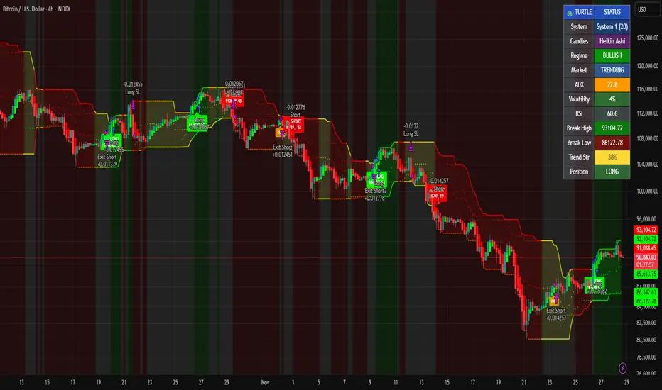
Third eye • StrategyThird eye • Strategy – User Guide
1. Idea & Concept
Third eye • Strategy combines three things into one system:
Ichimoku Cloud – to define market regime and support/resistance.
Moving Average (trend filter) – to trade only in the dominant direction.
CCI (Commodity Channel Index) – to generate precise entry signals on momentum breakouts.
The script is a strategy, not an indicator: it can backtest entries, exits, SL, TP and BreakEven logic automatically.
2. Indicators Used
2.1 Ichimoku
Standard Ichimoku settings (by default 9/26/52/26) are used:
Conversion Line (Tenkan-sen)
Base Line (Kijun-sen)
Leading Span A & B (Kumo Cloud)
Lagging Span is calculated but hidden from the chart (for visual simplicity).
From the cloud we derive:
kumoTop – top of the cloud under current price.
kumoBottom – bottom of the cloud under current price.
Flags:
is_above_kumo – price above the cloud.
is_below_kumo – price below the cloud.
is_in_kumo – price inside the cloud.
These conditions are used as trend / regime filters and for stop-loss & trailing stops.
2.2 Moving Average
You can optionally display and use a trend MA:
Types: SMA, EMA, DEMA, WMA
Length: configurable (default 200)
Source: default close
Filter idea:
If MA Direction Filter is ON:
When Close > MA → strategy allows only Long signals.
When Close < MA → strategy allows only Short signals.
The MA is plotted on the chart (if enabled).
2.3 CCI & Panel
The CCI (Commodity Channel Index) is used for entry timing:
CCI length and source are configurable (default length 20, source hlc3).
Two thresholds:
CCI Upper Threshold (Long) – default +100
CCI Lower Threshold (Short) – default –100
Signals:
Long signal:
CCI crosses up through the upper threshold
cci_val < upper_threshold and cci_val > upper_threshold
Short signal:
CCI crosses down through the lower threshold
cci_val > lower_threshold and cci_val < lower_threshold
There is a panel (table) in the bottom-right corner:
Shows current CCI value.
Shows filter status as colored dots:
Green = filter enabled and passed.
Red = filter enabled and blocking trades.
Gray = filter is disabled.
Filters shown in the panel:
Ichimoku Cloud filter (Long/Short)
Ichimoku Lines filter (Conversion/Base vs Cloud)
MA Direction filter
3. Filters & Trade Direction
All filters can be turned ON/OFF independently.
3.1 Ichimoku Cloud Filter
Purpose: trade only when price is clearly above or below the Kumo.
Long Cloud Filter (Use Ichimoku Cloud Filter) – when enabled:
Long trades only if close > cloud top.
Short Cloud Filter – when enabled:
Short trades only if close < cloud bottom.
If the cloud filter is disabled, this condition is ignored.
3.2 Ichimoku Lines Above/Below Cloud
Purpose: stronger trend confirmation: Ichimoku lines should also be on the “correct” side of the cloud.
Long Lines Filter:
Long allowed only if Conversion Line and Base Line are both above the cloud.
Short Lines Filter:
Short allowed only if both lines are below the cloud.
If this filter is OFF, the conditions are not checked.
3.3 MA Direction Filter
As described above:
When ON:
Close > MA → only Longs.
Close < MA → only Shorts.
4. Anti-Re-Entry Logic (Cloud Touch Reset)
The strategy uses internal flags to avoid continuous re-entries in the same direction without a reset.
Two flags:
allowLong
allowShort
After a Long entry, allowLong is set to false, allowShort to true.
After a Short entry, allowShort is set to false, allowLong to true.
Flags are reset when price touches the Kumo:
If Low goes into the cloud → allowLong = true
If High goes into the cloud → allowShort = true
If Close is inside the cloud → both allowLong and allowShort are set to true
There is a key option:
Wait Position Close Before Flag Reset
If ON: cloud touch will reset flags only when there is no open position.
If OFF: flags can be reset even while a trade is open.
This gives a kind of regime-based re-entry control: after a trend leg, you wait for a “cloud interaction” to allow new signals.
5. Risk Management
All risk management is handled inside the strategy.
5.1 Position Sizing
Order Size % of Equity – default 10%
The strategy calculates:
position_value = equity * (Order Size % / 100)
position_qty = position_value / close
So position size automatically adapts to your current equity.
5.2 Take Profit Modes
You can choose one of two TP modes:
Percent
Fibonacci
5.2.1 Percent Mode
Single Take Profit at X% from entry (default 2%).
For Long:
TP = entry_price * (1 + tp_pct / 100)
For Short:
TP = entry_price * (1 - tp_pct / 100)
One strategy.exit per side is used: "Long TP/SL" and "Short TP/SL".
5.2.2 Fibonacci Mode (2 partial TPs)
In this mode, TP levels are based on a virtual Fib-style extension between entry and stop-loss.
Inputs:
Fib TP1 Level (default 1.618)
Fib TP2 Level (default 2.5)
TP1 Share % (Fib) (default 50%)
TP2 share is automatically 100% - TP1 share.
Process for Long:
Compute a reference Stop (see SL section below) → sl_for_fib.
Compute distance: dist = entry_price - sl_for_fib.
TP levels:
TP1 = entry_price + dist * (Fib TP1 Level - 1)
TP2 = entry_price + dist * (Fib TP2 Level - 1)
For Short, the logic is mirrored.
Two exits are used:
TP1 – closes TP1 share % of position.
TP2 – closes remaining TP2 share %.
Same stop is used for both partial exits.
5.3 Stop-Loss Modes
You can choose one of three Stop Loss modes:
Stable – fixed % from entry.
Ichimoku – fixed level derived from the Kumo.
Ichimoku Trailing – dynamic SL following the cloud.
5.3.1 Stable SL
For Long:
SL = entry_price * (1 - Stable SL % / 100)
For Short:
SL = entry_price * (1 + Stable SL % / 100)
Used both for Percent TP mode and as reference for Fib TP if Kumo is not available.
5.3.2 Ichimoku SL (fixed, non-trailing)
At the time of a new trade:
For Long:
Base SL = cloud bottom minus small offset (%)
For Short:
Base SL = cloud top plus small offset (%)
The offset is configurable: Ichimoku SL Offset %.
Once computed, that SL level is fixed for this trade.
5.3.3 Ichimoku Trailing SL
Similar to Ichimoku SL, but recomputed each bar:
For Long:
SL = cloud bottom – offset
For Short:
SL = cloud top + offset
A red trailing SL line is drawn on the chart to visualize current stop level.
This trailing SL is also used as reference for BreakEven and for Fib TP distance.
6. BreakEven Logic (with BE Lines)
BreakEven is optional and supports two modes:
Percent
Fibonacci
Inputs:
Percent mode:
BE Trigger % (from entry) – move SL to BE when price goes this % in profit.
BE Offset % from entry – SL will be set to entry ± this offset.
Fibonacci mode:
BE Fib Level – Fib level at which BE will be activated (default 1.618, same style as TP).
BE Offset % from entry – how far from entry to place BE stop.
The logic:
Before BE is triggered, SL follows its normal mode (Stable/Ichimoku/Ichimoku Trailing).
When BE triggers:
For Long:
New SL = max(current SL, BE SL).
For Short:
New SL = min(current SL, BE SL).
This means BE will never loosen the stop – only tighten it.
When BE is activated, the strategy draws a violet horizontal line at the BreakEven level (once per trade).
BE state is cleared when the position is closed or when a new position is opened.
7. Entry & Exit Logic (Summary)
7.1 Long Entry
Conditions for a Long:
CCI signal:
CCI crosses up through the upper threshold.
Ichimoku Cloud Filter (optional):
If enabled → price must be above the Kumo.
Ichimoku Lines Filter (optional):
If enabled → Conversion Line and Base Line must be above the Kumo.
MA Direction Filter (optional):
If enabled → Close must be above the chosen MA.
Anti-re-entry flag:
allowLong must be true (cloud-based reset).
Position check:
Long entries are allowed when current position size ≤ 0 (so it can also reverse from short to long).
If all these conditions are true, the strategy sends:
strategy.entry("Long", strategy.long, qty = calculated_qty)
After entry:
allowLong = false
allowShort = true
7.2 Short Entry
Same structure, mirrored:
CCI signal:
CCI crosses down through the lower threshold.
Cloud filter: price must be below cloud (if enabled).
Lines filter: conversion & base must be below cloud (if enabled).
MA filter: Close must be below MA (if enabled).
allowShort must be true.
Position check: position size ≥ 0 (allows reversal from long to short).
Then:
strategy.entry("Short", strategy.short, qty = calculated_qty)
Flags update:
allowShort = false
allowLong = true
7.3 Exits
While in a position:
The strategy continuously recalculates SL (depending on chosen mode) and, in Percent mode, TP.
In Fib mode, fixed TP levels are computed at entry.
BreakEven may raise/tighten the SL if its conditions are met.
Exits are executed via strategy.exit:
Percent mode: one TP+SL exit per side.
Fib mode: two partial exits (TP1 and TP2) sharing the same SL.
At position open, the script also draws visual lines:
White line — entry price.
Green line(s) — TP level(s).
Red line — SL (if not using Ichimoku Trailing; with trailing, the red line is updated dynamically).
Maximum of 30 lines are kept to avoid clutter.
8. How to Use the Strategy
Choose market & timeframe
Works well on trending instruments. Try crypto, FX or indices on H1–H4, or intraday if you prefer more trades.
Adjust Ichimoku settings
Keep defaults (9/26/52/26) or adapt to your timeframe.
Configure Moving Average
Typical: EMA 200 as a trend filter.
Turn MA Direction Filter ON if you want to trade only with the main trend.
Set CCI thresholds
Default ±100 is classic.
Lower thresholds → more signals, higher noise.
Higher thresholds → fewer but stronger signals.
Enable/disable filters
Turn on Ichimoku Cloud and Ichimoku Lines if you want only “clean” trend trades.
Use Wait Position Close Before Flag Reset to control how often re-entries are allowed.
Choose TP & SL mode
Percent mode is simpler and easier to understand.
Fibonacci mode is more advanced: it aligns TP levels with the distance to stop, giving asymmetric RR setups (two partial TPs).
Choose Stable SL for fixed-risk trades, or Ichimoku / Ichimoku Trailing to tie stops to the cloud structure.
Set BreakEven
Enable BE if you want to lock in risk-free trades after a certain move.
Percent mode is straightforward; Fib mode keeps BreakEven in harmony with your Fib TP setup.
Run Backtest & Optimize
Press “Add to chart” → go to Strategy Tester.
Adjust parameters to your market and timeframe.
Look at equity curve, PF, drawdown, average trade, etc.
Live / Paper Trading
After you’re satisfied with backtest results, use the strategy to generate signals.
You can mirror entries/exits manually or connect them to alerts (if you build an alert-based execution layer).

Bassi's Consolidation Breakout — ULTIMATE PRO + VPOverview
Bassi’s Consolidation Breakout — ULTIMATE PRO + VP is a professional-grade breakout detection system that combines price structure, volume confirmation, volatility compression, and custom volume profile logic.
The indicator automatically detects compressed consolidation zones, confirms breakouts with multi-layer filters, and plots full trade setups including:
Entry level
Stop-loss
TP1, TP2, TP3 (R:R based)
Trend filters + MTF EMA
Retest validation
Volume Profile confirmation (POC / VAH / VAL)
This is one of the most complete breakout frameworks for TradingView.
🔍 Core Concept
The script detects tight consolidation boxes based on:
Price range (% compression)
Lookback period
Minimum required bars
Breakout above/below the box
Once the consolidation ends, breakout signals fire only if they pass all filters.
This focuses your trading on high-probability breakouts only.
🔥 Key Features
1️⃣ Automated Consolidation Box Detection
Draws consolidation boxes dynamically
Identifies tight range compression
Supports advanced range logic for high accuracy
2️⃣ Smart Breakout + Retest Engine
Breakouts and breakdowns require:
Structure break
Minimum breakout expansion (0.15%)
Volume confirmation
Trend (200 EMA) confirmation
Optional retest validation
Optional Volume Profile filter
Each valid breakout prints a signal + full trade setup.
3️⃣ Custom Volume Profile Engine
Fast and lightweight custom-built VP that calculates:
POC (Point of Control)
VAH (Value Area High)
VAL (Value Area Low)
These levels can optionally be used to filter weak breakouts.
4️⃣ Multi-Timeframe Trend Filter
Uses 200 EMA from any selected higher timeframe
Helps avoid counter-trend fakeouts
Fully optional
5️⃣ Automatic Trade Setup Projection
Each breakout generates:
Stop-loss (ATR × multiplier)
TP1 (R:R)
TP2 (R:R)
TP3 (optional)
Clean signal labels
Only keeps the last 2 signals to maintain clarity
6️⃣ Alerts Included
Alerts fire instantly when a valid breakout occurs:
“Bassi LONG + VP”
“Bassi SHORT + VP”
Alerts include ticker + entry price.
📘 Usage Guide & Trading Rules
✔ Recommended Trading Steps
1. Wait for a confirmed consolidation box
Box must be narrow
Must meet minimum bar requirement
2. Wait for a confirmed breakout signal
Signal requires:
Breakout above/below box
Volume confirmation
Trend & MTF confirmation if enabled
Optional retest
Optional VP filter (close outside VAH/VAL)
3. Follow the projected setup
The script prints:
Entry
SL
TP1 / TP2 / TP3
Target lines extend automatically.
📖 How to Use the Script (Trading Rules)
1️⃣ Long Entry Rules
Enter Long when:
Price breaks above trend confirmation level
Momentum signal turns bullish
Candle closes above trigger line
Volatility filter is satisfied
Exit Long:
TP1/TP2/TP3 levels
Reversal signal
Trailing stop hit
2️⃣ Short Entry Rules
Enter Short when:
Price breaks below trend confirmation level
Momentum signal turns bearish
Candle closes below trigger line
Volatility filter is satisfied
Exit Short:
TP1/TP2/TP3 levels
Trend reversal
Trailing stop hit
✔ Recommended Markets
Crypto
Forex
Indices
Futures
Stocks
Works on all timeframes from 1-minute to daily.
✔ Best Practice
Avoid taking signals against HTF trend
Prefer signals that break away from VAH/VAL
Use TP1 to secure partial profits
Move SL to breakeven after TP1 if desired
Always follow personal risk management
👤 Author
Created by: Mahdi Bassi
Professional trader & systems designer
Focused on structural, volume-based and volatility-based strategies.
⚠️ Disclaimer
This script is for educational purposes only.
No indicator can guarantee profits.
Always use proper risk management and trade responsibly.

Stratégie SMC V18.2 (BTC/EUR FINAL R3 - Tendance)This strategy is an automated implementation of Smart Money Concepts (SMC), designed to operate on the Bitcoin/Euro (BTC/EUR) chart using the 15-minute Timeframe (M15).It focuses on identifying high-probability zones (Order Blocks) after a confirmed Break of Structure (BOS) and a Liquidity Sweep, utilizing an H1/EMA 200 trend filter to only execute trades in the direction of the dominant market flow.Risk management is strict: every trade uses a fixed Risk-to-Reward Ratio (R:R) of 1:3.🧱 Core Logic Components
1. Trend Filter (H1/EMA 200)Objective: To avoid counter-trend entries, which has allowed the success rate to increase to nearly $65\%$ in backtests.Mechanism: A $200$-period EMA is plotted on a higher timeframe (Default: H1/60 minutes).Long (Buy): Entry is only permitted if the current price (M15) is above the trend EMA.Short (Sell): Entry is only permitted if the current price (M15) is below the trend EMA.
2. Order Block (OB) DetectionA potential Order Block is identified on the previous candle if it is
accompanied by an inefficiency (FVG - Fair Value Gap).
3. Advanced SMC ValidationBOS (Break of Structure): A recent BOS must be confirmed by breaking the swing high/low defined by the swing length (Default: 4 M15 candles).Liquidity (Liquidity Sweep): The Order Block zone must have swept recent liquidity (defined by the Liquidity Search Length) within a certain tolerance (Default: $0.1\%$).Point of Interest: The OB must form in a premium zone (for shorts) or a discount zone (for longs) relative to the current swing range (above or below the $50\%$ level of the range).
4. Execution and Risk ManagementEntry: The trade is triggered when the price touches the active Order Block (mitigation).Stop Loss (SL): The SL is fixed at the low of the OB (for longs) or the high of the OB (for shorts).Take Profit (TP): The TP is strictly set at a level corresponding to 3 times the SL distance (R:R 1:3).Lot Sizing: The trade quantity is calculated to risk a fixed amount (Default: 2.00 Euros) per transaction, capped by a Lot Max and Lot Min defined by the user.
Input Parameters (Optimized for BTC/EUR M15)Users can adjust these parameters to modify sensitivity and risk profile. The default values are those optimized for the high-performing backtest (Profit Factor $> 3$).ParameterDescriptionDefault Value (M15)Long. Swing (BOS)Candle length used to define the swing (and thus the BOS).4Long. Recherche Liq.Number of candles to scan to confirm a liquidity sweep.7Tolérance Liq. (%)Price tolerance to validate the liquidity sweep (as a percentage of price).0.1Timeframe TendanceChart timeframe used for the EMA filter (e.g., 60 = H1).60 (H1)Longueur EMA TendancePeriods used for the trend EMA.200Lot Max (Quantité Max BTC)Maximum quantity of BTC the strategy is allowed to trade.0.01Lot Min Réel (Exigence Broker)Minimum quantity required by the broker/exchange.0.00001

Roshan Dash Ultimate Trading DashboardHas the key moving averages sma (10,20,50,200) in daily and above timeframe. And for lower timeframe it has ema (10,20,50,200) and vwap. Displays key information like marketcap, sector, lod%, atr, atr% and distance of atr from 50sma . All things which help determine whether or not to take trade.

Multi EMA and SMA with VWAP Indicator📊 Custom Multi-MA & VWAP Indicator
A comprehensive and fully customizable moving average indicator that combines 6 Exponential Moving Averages (EMAs), 3 Simple Moving Averages (SMAs), and VWAP in one clean, easy-to-use tool.
✨ Features:
6 Configurable EMAs:
• Default periods: 9, 21, 50, 100, 150, 200
• Fully adjustable lengths
• Individual color customization
• Show/hide toggles for each EMA
3 Configurable SMAs:
• Default periods: 20, 50, 100
• Fully adjustable lengths
• Individual color customization
• Show/hide toggles for each SMA
• Thicker lines for easy distinction from EMAs
VWAP (Volume Weighted Average Price):
• Toggle on/off
• Customizable color and line width
• Essential for intraday trading and institutional levels
🎯 Use Cases:
• Trend identification and confirmation
• Support and resistance levels
• Entry and exit signals
• Multi-timeframe analysis
• Day trading and swing trading strategies
• Institutional price levels (VWAP)
⚙️ Fully Customizable:
Every aspect of this indicator is configurable through the settings panel:
• Adjust any MA period to fit your trading strategy
• Choose your preferred colors for better chart visualization
• Enable/disable specific MAs to reduce chart clutter
• Customize VWAP line thickness
📈 Perfect For:
• Traders who use multiple moving averages in their strategy
• Those seeking an all-in-one MA solution
• Clean chart organization with one indicator instead of multiple
• Both beginners and experienced traders
💡 Tips:
• Use shorter EMAs (9, 21) for quick trend changes
• Longer EMAs (100, 150, 200) act as strong support/resistance
• VWAP is particularly useful for intraday trading
• Customize colors to match your chart theme
Version: Pine Script v6
Overlay: Yes (plots directly on price chart)

Dimensional Resonance ProtocolDimensional Resonance Protocol
🌀 CORE INNOVATION: PHASE SPACE RECONSTRUCTION & EMERGENCE DETECTION
The Dimensional Resonance Protocol represents a paradigm shift from traditional technical analysis to complexity science. Rather than measuring price levels or indicator crossovers, DRP reconstructs the hidden attractor governing market dynamics using Takens' embedding theorem, then detects emergence —the rare moments when multiple dimensions of market behavior spontaneously synchronize into coherent, predictable states.
The Complexity Hypothesis:
Markets are not simple oscillators or random walks—they are complex adaptive systems existing in high-dimensional phase space. Traditional indicators see only shadows (one-dimensional projections) of this higher-dimensional reality. DRP reconstructs the full phase space using time-delay embedding, revealing the true structure of market dynamics.
Takens' Embedding Theorem (1981):
A profound mathematical result from dynamical systems theory: Given a time series from a complex system, we can reconstruct its full phase space by creating delayed copies of the observation.
Mathematical Foundation:
From single observable x(t), create embedding vectors:
X(t) =
Where:
• d = Embedding dimension (default 5)
• τ = Time delay (default 3 bars)
• x(t) = Price or return at time t
Key Insight: If d ≥ 2D+1 (where D is the true attractor dimension), this embedding is topologically equivalent to the actual system dynamics. We've reconstructed the hidden attractor from a single price series.
Why This Matters:
Markets appear random in one dimension (price chart). But in reconstructed phase space, structure emerges—attractors, limit cycles, strange attractors. When we identify these structures, we can detect:
• Stable regions : Predictable behavior (trade opportunities)
• Chaotic regions : Unpredictable behavior (avoid trading)
• Critical transitions : Phase changes between regimes
Phase Space Magnitude Calculation:
phase_magnitude = sqrt(Σ ² for i = 0 to d-1)
This measures the "energy" or "momentum" of the market trajectory through phase space. High magnitude = strong directional move. Low magnitude = consolidation.
📊 RECURRENCE QUANTIFICATION ANALYSIS (RQA)
Once phase space is reconstructed, we analyze its recurrence structure —when does the system return near previous states?
Recurrence Plot Foundation:
A recurrence occurs when two phase space points are closer than threshold ε:
R(i,j) = 1 if ||X(i) - X(j)|| < ε, else 0
This creates a binary matrix showing when the system revisits similar states.
Key RQA Metrics:
1. Recurrence Rate (RR):
RR = (Number of recurrent points) / (Total possible pairs)
• RR near 0: System never repeats (highly stochastic)
• RR = 0.1-0.3: Moderate recurrence (tradeable patterns)
• RR > 0.5: System stuck in attractor (ranging market)
• RR near 1: System frozen (no dynamics)
Interpretation: Moderate recurrence is optimal —patterns exist but market isn't stuck.
2. Determinism (DET):
Measures what fraction of recurrences form diagonal structures in the recurrence plot. Diagonals indicate deterministic evolution (trajectory follows predictable paths).
DET = (Recurrence points on diagonals) / (Total recurrence points)
• DET < 0.3: Random dynamics
• DET = 0.3-0.7: Moderate determinism (patterns with noise)
• DET > 0.7: Strong determinism (technical patterns reliable)
Trading Implication: Signals are prioritized when DET > 0.3 (deterministic state) and RR is moderate (not stuck).
Threshold Selection (ε):
Default ε = 0.10 × std_dev means two states are "recurrent" if within 10% of a standard deviation. This is tight enough to require genuine similarity but loose enough to find patterns.
🔬 PERMUTATION ENTROPY: COMPLEXITY MEASUREMENT
Permutation entropy measures the complexity of a time series by analyzing the distribution of ordinal patterns.
Algorithm (Bandt & Pompe, 2002):
1. Take overlapping windows of length n (default n=4)
2. For each window, record the rank order pattern
Example: → pattern (ranks from lowest to highest)
3. Count frequency of each possible pattern
4. Calculate Shannon entropy of pattern distribution
Mathematical Formula:
H_perm = -Σ p(π) · ln(p(π))
Where π ranges over all n! possible permutations, p(π) is the probability of pattern π.
Normalized to :
H_norm = H_perm / ln(n!)
Interpretation:
• H < 0.3 : Very ordered, crystalline structure (strong trending)
• H = 0.3-0.5 : Ordered regime (tradeable with patterns)
• H = 0.5-0.7 : Moderate complexity (mixed conditions)
• H = 0.7-0.85 : Complex dynamics (challenging to trade)
• H > 0.85 : Maximum entropy (nearly random, avoid)
Entropy Regime Classification:
DRP classifies markets into five entropy regimes:
• CRYSTALLINE (H < 0.3): Maximum order, persistent trends
• ORDERED (H < 0.5): Clear patterns, momentum strategies work
• MODERATE (H < 0.7): Mixed dynamics, adaptive required
• COMPLEX (H < 0.85): High entropy, mean reversion better
• CHAOTIC (H ≥ 0.85): Near-random, minimize trading
Why Permutation Entropy?
Unlike traditional entropy methods requiring binning continuous data (losing information), permutation entropy:
• Works directly on time series
• Robust to monotonic transformations
• Computationally efficient
• Captures temporal structure, not just distribution
• Immune to outliers (uses ranks, not values)
⚡ LYAPUNOV EXPONENT: CHAOS vs STABILITY
The Lyapunov exponent λ measures sensitivity to initial conditions —the hallmark of chaos.
Physical Meaning:
Two trajectories starting infinitely close will diverge at exponential rate e^(λt):
Distance(t) ≈ Distance(0) × e^(λt)
Interpretation:
• λ > 0 : Positive Lyapunov exponent = CHAOS
- Small errors grow exponentially
- Long-term prediction impossible
- System is sensitive, unpredictable
- AVOID TRADING
• λ ≈ 0 : Near-zero = CRITICAL STATE
- Edge of chaos
- Transition zone between order and disorder
- Moderate predictability
- PROCEED WITH CAUTION
• λ < 0 : Negative Lyapunov exponent = STABLE
- Small errors decay
- Trajectories converge
- System is predictable
- OPTIMAL FOR TRADING
Estimation Method:
DRP estimates λ by tracking how quickly nearby states diverge over a rolling window (default 20 bars):
For each bar i in window:
δ₀ = |x - x | (initial separation)
δ₁ = |x - x | (previous separation)
if δ₁ > 0:
ratio = δ₀ / δ₁
log_ratios += ln(ratio)
λ ≈ average(log_ratios)
Stability Classification:
• STABLE : λ < 0 (negative growth rate)
• CRITICAL : |λ| < 0.1 (near neutral)
• CHAOTIC : λ > 0.2 (strong positive growth)
Signal Filtering:
By default, NEXUS requires λ < 0 (stable regime) for signal confirmation. This filters out trades during chaotic periods when technical patterns break down.
📐 HIGUCHI FRACTAL DIMENSION
Fractal dimension measures self-similarity and complexity of the price trajectory.
Theoretical Background:
A curve's fractal dimension D ranges from 1 (smooth line) to 2 (space-filling curve):
• D ≈ 1.0 : Smooth, persistent trending
• D ≈ 1.5 : Random walk (Brownian motion)
• D ≈ 2.0 : Highly irregular, space-filling
Higuchi Method (1988):
For a time series of length N, construct k different curves by taking every k-th point:
L(k) = (1/k) × Σ|x - x | × (N-1)/(⌊(N-m)/k⌋ × k)
For different values of k (1 to k_max), calculate L(k). The fractal dimension is the slope of log(L(k)) vs log(1/k):
D = slope of log(L) vs log(1/k)
Market Interpretation:
• D < 1.35 : Strong trending, persistent (Hurst > 0.5)
- TRENDING regime
- Momentum strategies favored
- Breakouts likely to continue
• D = 1.35-1.45 : Moderate persistence
- PERSISTENT regime
- Trend-following with caution
- Patterns have meaning
• D = 1.45-1.55 : Random walk territory
- RANDOM regime
- Efficiency hypothesis holds
- Technical analysis least reliable
• D = 1.55-1.65 : Anti-persistent (mean-reverting)
- ANTI-PERSISTENT regime
- Oscillator strategies work
- Overbought/oversold meaningful
• D > 1.65 : Highly complex, choppy
- COMPLEX regime
- Avoid directional bets
- Wait for regime change
Signal Filtering:
Resonance signals (secondary signal type) require D < 1.5, indicating trending or persistent dynamics where momentum has meaning.
🔗 TRANSFER ENTROPY: CAUSAL INFORMATION FLOW
Transfer entropy measures directed causal influence between time series—not just correlation, but actual information transfer.
Schreiber's Definition (2000):
Transfer entropy from X to Y measures how much knowing X's past reduces uncertainty about Y's future:
TE(X→Y) = H(Y_future | Y_past) - H(Y_future | Y_past, X_past)
Where H is Shannon entropy.
Key Properties:
1. Directional : TE(X→Y) ≠ TE(Y→X) in general
2. Non-linear : Detects complex causal relationships
3. Model-free : No assumptions about functional form
4. Lag-independent : Captures delayed causal effects
Three Causal Flows Measured:
1. Volume → Price (TE_V→P):
Measures how much volume patterns predict price changes.
• TE > 0 : Volume provides predictive information about price
- Institutional participation driving moves
- Volume confirms direction
- High reliability
• TE ≈ 0 : No causal flow (weak volume/price relationship)
- Volume uninformative
- Caution on signals
• TE < 0 (rare): Suggests price leading volume
- Potentially manipulated or thin market
2. Volatility → Momentum (TE_σ→M):
Does volatility expansion predict momentum changes?
• Positive TE : Volatility precedes momentum shifts
- Breakout dynamics
- Regime transitions
3. Structure → Price (TE_S→P):
Do support/resistance patterns causally influence price?
• Positive TE : Structural levels have causal impact
- Technical levels matter
- Market respects structure
Net Causal Flow:
Net_Flow = TE_V→P + 0.5·TE_σ→M + TE_S→P
• Net > +0.1 : Bullish causal structure
• Net < -0.1 : Bearish causal structure
• |Net| < 0.1 : Neutral/unclear causation
Causal Gate:
For signal confirmation, NEXUS requires:
• Buy signals : TE_V→P > 0 AND Net_Flow > 0.05
• Sell signals : TE_V→P > 0 AND Net_Flow < -0.05
This ensures volume is actually driving price (causal support exists), not just correlated noise.
Implementation Note:
Computing true transfer entropy requires discretizing continuous data into bins (default 6 bins) and estimating joint probability distributions. NEXUS uses a hybrid approach combining TE theory with autocorrelation structure and lagged cross-correlation to approximate information transfer in computationally efficient manner.
🌊 HILBERT PHASE COHERENCE
Phase coherence measures synchronization across market dimensions using Hilbert transform analysis.
Hilbert Transform Theory:
For a signal x(t), the Hilbert transform H (t) creates an analytic signal:
z(t) = x(t) + i·H (t) = A(t)·e^(iφ(t))
Where:
• A(t) = Instantaneous amplitude
• φ(t) = Instantaneous phase
Instantaneous Phase:
φ(t) = arctan(H (t) / x(t))
The phase represents where the signal is in its natural cycle—analogous to position on a unit circle.
Four Dimensions Analyzed:
1. Momentum Phase : Phase of price rate-of-change
2. Volume Phase : Phase of volume intensity
3. Volatility Phase : Phase of ATR cycles
4. Structure Phase : Phase of position within range
Phase Locking Value (PLV):
For two signals with phases φ₁(t) and φ₂(t), PLV measures phase synchronization:
PLV = |⟨e^(i(φ₁(t) - φ₂(t)))⟩|
Where ⟨·⟩ is time average over window.
Interpretation:
• PLV = 0 : Completely random phase relationship (no synchronization)
• PLV = 0.5 : Moderate phase locking
• PLV = 1 : Perfect synchronization (phases locked)
Pairwise PLV Calculations:
• PLV_momentum-volume : Are momentum and volume cycles synchronized?
• PLV_momentum-structure : Are momentum cycles aligned with structure?
• PLV_volume-structure : Are volume and structural patterns in phase?
Overall Phase Coherence:
Coherence = (PLV_mom-vol + PLV_mom-struct + PLV_vol-struct) / 3
Signal Confirmation:
Emergence signals require coherence ≥ threshold (default 0.70):
• Below 0.70: Dimensions not synchronized, no coherent market state
• Above 0.70: Dimensions in phase, coherent behavior emerging
Coherence Direction:
The summed phase angles indicate whether synchronized dimensions point bullish or bearish:
Direction = sin(φ_momentum) + 0.5·sin(φ_volume) + 0.5·sin(φ_structure)
• Direction > 0 : Phases pointing upward (bullish synchronization)
• Direction < 0 : Phases pointing downward (bearish synchronization)
🌀 EMERGENCE SCORE: MULTI-DIMENSIONAL ALIGNMENT
The emergence score aggregates all complexity metrics into a single 0-1 value representing market coherence.
Eight Components with Weights:
1. Phase Coherence (20%):
Direct contribution: coherence × 0.20
Measures dimensional synchronization.
2. Entropy Regime (15%):
Contribution: (0.6 - H_perm) / 0.6 × 0.15 if H < 0.6, else 0
Rewards low entropy (ordered, predictable states).
3. Lyapunov Stability (12%):
• λ < 0 (stable): +0.12
• |λ| < 0.1 (critical): +0.08
• λ > 0.2 (chaotic): +0.0
Requires stable, predictable dynamics.
4. Fractal Dimension Trending (12%):
Contribution: (1.45 - D) / 0.45 × 0.12 if D < 1.45, else 0
Rewards trending fractal structure (D < 1.45).
5. Dimensional Resonance (12%):
Contribution: |dimensional_resonance| × 0.12
Measures alignment across momentum, volume, structure, volatility dimensions.
6. Causal Flow Strength (9%):
Contribution: |net_causal_flow| × 0.09
Rewards strong causal relationships.
7. Phase Space Embedding (10%):
Contribution: min(|phase_magnitude_norm|, 3.0) / 3.0 × 0.10 if |magnitude| > 1.0
Rewards strong trajectory in reconstructed phase space.
8. Recurrence Quality (10%):
Contribution: determinism × 0.10 if DET > 0.3 AND 0.1 < RR < 0.8
Rewards deterministic patterns with moderate recurrence.
Total Emergence Score:
E = Σ(components) ∈
Capped at 1.0 maximum.
Emergence Direction:
Separate calculation determining bullish vs bearish:
• Dimensional resonance sign
• Net causal flow sign
• Phase magnitude correlation with momentum
Signal Threshold:
Default emergence_threshold = 0.75 means 75% of maximum possible emergence score required to trigger signals.
Why Emergence Matters:
Traditional indicators measure single dimensions. Emergence detects self-organization —when multiple independent dimensions spontaneously align. This is the market equivalent of a phase transition in physics, where microscopic chaos gives way to macroscopic order.
These are the highest-probability trade opportunities because the entire system is resonating in the same direction.
🎯 SIGNAL GENERATION: EMERGENCE vs RESONANCE
DRP generates two tiers of signals with different requirements:
TIER 1: EMERGENCE SIGNALS (Primary)
Requirements:
1. Emergence score ≥ threshold (default 0.75)
2. Phase coherence ≥ threshold (default 0.70)
3. Emergence direction > 0.2 (bullish) or < -0.2 (bearish)
4. Causal gate passed (if enabled): TE_V→P > 0 and net_flow confirms direction
5. Stability zone (if enabled): λ < 0 or |λ| < 0.1
6. Price confirmation: Close > open (bulls) or close < open (bears)
7. Cooldown satisfied: bars_since_signal ≥ cooldown_period
EMERGENCE BUY:
• All above conditions met with bullish direction
• Market has achieved coherent bullish state
• Multiple dimensions synchronized upward
EMERGENCE SELL:
• All above conditions met with bearish direction
• Market has achieved coherent bearish state
• Multiple dimensions synchronized downward
Premium Emergence:
When signal_quality (emergence_score × phase_coherence) > 0.7:
• Displayed as ★ star symbol
• Highest conviction trades
• Maximum dimensional alignment
Standard Emergence:
When signal_quality 0.5-0.7:
• Displayed as ◆ diamond symbol
• Strong signals but not perfect alignment
TIER 2: RESONANCE SIGNALS (Secondary)
Requirements:
1. Dimensional resonance > +0.6 (bullish) or < -0.6 (bearish)
2. Fractal dimension < 1.5 (trending/persistent regime)
3. Price confirmation matches direction
4. NOT in chaotic regime (λ < 0.2)
5. Cooldown satisfied
6. NO emergence signal firing (resonance is fallback)
RESONANCE BUY:
• Dimensional alignment without full emergence
• Trending fractal structure
• Moderate conviction
RESONANCE SELL:
• Dimensional alignment without full emergence
• Bearish resonance with trending structure
• Moderate conviction
Displayed as small ▲/▼ triangles with transparency.
Signal Hierarchy:
IF emergence conditions met:
Fire EMERGENCE signal (★ or ◆)
ELSE IF resonance conditions met:
Fire RESONANCE signal (▲ or ▼)
ELSE:
No signal
Cooldown System:
After any signal fires, cooldown_period (default 5 bars) must elapse before next signal. This prevents signal clustering during persistent conditions.
Cooldown tracks using bar_index:
bars_since_signal = current_bar_index - last_signal_bar_index
cooldown_ok = bars_since_signal >= cooldown_period
🎨 VISUAL SYSTEM: MULTI-LAYER COMPLEXITY
DRP provides rich visual feedback across four distinct layers:
LAYER 1: COHERENCE FIELD (Background)
Colored background intensity based on phase coherence:
• No background : Coherence < 0.5 (incoherent state)
• Faint glow : Coherence 0.5-0.7 (building coherence)
• Stronger glow : Coherence > 0.7 (coherent state)
Color:
• Cyan/teal: Bullish coherence (direction > 0)
• Red/magenta: Bearish coherence (direction < 0)
• Blue: Neutral coherence (direction ≈ 0)
Transparency: 98 minus (coherence_intensity × 10), so higher coherence = more visible.
LAYER 2: STABILITY/CHAOS ZONES
Background color indicating Lyapunov regime:
• Green tint (95% transparent): λ < 0, STABLE zone
- Safe to trade
- Patterns meaningful
• Gold tint (90% transparent): |λ| < 0.1, CRITICAL zone
- Edge of chaos
- Moderate risk
• Red tint (85% transparent): λ > 0.2, CHAOTIC zone
- Avoid trading
- Unpredictable behavior
LAYER 3: DIMENSIONAL RIBBONS
Three EMAs representing dimensional structure:
• Fast ribbon : EMA(8) in cyan/teal (fast dynamics)
• Medium ribbon : EMA(21) in blue (intermediate)
• Slow ribbon : EMA(55) in red/magenta (slow dynamics)
Provides visual reference for multi-scale structure without cluttering with raw phase space data.
LAYER 4: CAUSAL FLOW LINE
A thicker line plotted at EMA(13) colored by net causal flow:
• Cyan/teal : Net_flow > +0.1 (bullish causation)
• Red/magenta : Net_flow < -0.1 (bearish causation)
• Gray : |Net_flow| < 0.1 (neutral causation)
Shows real-time direction of information flow.
EMERGENCE FLASH:
Strong background flash when emergence signals fire:
• Cyan flash for emergence buy
• Red flash for emergence sell
• 80% transparency for visibility without obscuring price
📊 COMPREHENSIVE DASHBOARD
Real-time monitoring of all complexity metrics:
HEADER:
• 🌀 DRP branding with gold accent
CORE METRICS:
EMERGENCE:
• Progress bar (█ filled, ░ empty) showing 0-100%
• Percentage value
• Direction arrow (↗ bull, ↘ bear, → neutral)
• Color-coded: Green/gold if active, gray if low
COHERENCE:
• Progress bar showing phase locking value
• Percentage value
• Checkmark ✓ if ≥ threshold, circle ○ if below
• Color-coded: Cyan if coherent, gray if not
COMPLEXITY SECTION:
ENTROPY:
• Regime name (CRYSTALLINE/ORDERED/MODERATE/COMPLEX/CHAOTIC)
• Numerical value (0.00-1.00)
• Color: Green (ordered), gold (moderate), red (chaotic)
LYAPUNOV:
• State (STABLE/CRITICAL/CHAOTIC)
• Numerical value (typically -0.5 to +0.5)
• Status indicator: ● stable, ◐ critical, ○ chaotic
• Color-coded by state
FRACTAL:
• Regime (TRENDING/PERSISTENT/RANDOM/ANTI-PERSIST/COMPLEX)
• Dimension value (1.0-2.0)
• Color: Cyan (trending), gold (random), red (complex)
PHASE-SPACE:
• State (STRONG/ACTIVE/QUIET)
• Normalized magnitude value
• Parameters display: d=5 τ=3
CAUSAL SECTION:
CAUSAL:
• Direction (BULL/BEAR/NEUTRAL)
• Net flow value
• Flow indicator: →P (to price), P← (from price), ○ (neutral)
V→P:
• Volume-to-price transfer entropy
• Small display showing specific TE value
DIMENSIONAL SECTION:
RESONANCE:
• Progress bar of absolute resonance
• Signed value (-1 to +1)
• Color-coded by direction
RECURRENCE:
• Recurrence rate percentage
• Determinism percentage display
• Color-coded: Green if high quality
STATE SECTION:
STATE:
• Current mode: EMERGENCE / RESONANCE / CHAOS / SCANNING
• Icon: 🚀 (emergence buy), 💫 (emergence sell), ▲ (resonance buy), ▼ (resonance sell), ⚠ (chaos), ◎ (scanning)
• Color-coded by state
SIGNALS:
• E: count of emergence signals
• R: count of resonance signals
⚙️ KEY PARAMETERS EXPLAINED
Phase Space Configuration:
• Embedding Dimension (3-10, default 5): Reconstruction dimension
- Low (3-4): Simple dynamics, faster computation
- Medium (5-6): Balanced (recommended)
- High (7-10): Complex dynamics, more data needed
- Rule: d ≥ 2D+1 where D is true dimension
• Time Delay (τ) (1-10, default 3): Embedding lag
- Fast markets: 1-2
- Normal: 3-4
- Slow markets: 5-10
- Optimal: First minimum of mutual information (often 2-4)
• Recurrence Threshold (ε) (0.01-0.5, default 0.10): Phase space proximity
- Tight (0.01-0.05): Very similar states only
- Medium (0.08-0.15): Balanced
- Loose (0.20-0.50): Liberal matching
Entropy & Complexity:
• Permutation Order (3-7, default 4): Pattern length
- Low (3): 6 patterns, fast but coarse
- Medium (4-5): 24-120 patterns, balanced
- High (6-7): 720-5040 patterns, fine-grained
- Note: Requires window >> order! for stability
• Entropy Window (15-100, default 30): Lookback for entropy
- Short (15-25): Responsive to changes
- Medium (30-50): Stable measure
- Long (60-100): Very smooth, slow adaptation
• Lyapunov Window (10-50, default 20): Stability estimation window
- Short (10-15): Fast chaos detection
- Medium (20-30): Balanced
- Long (40-50): Stable λ estimate
Causal Inference:
• Enable Transfer Entropy (default ON): Causality analysis
- Keep ON for full system functionality
• TE History Length (2-15, default 5): Causal lookback
- Short (2-4): Quick causal detection
- Medium (5-8): Balanced
- Long (10-15): Deep causal analysis
• TE Discretization Bins (4-12, default 6): Binning granularity
- Few (4-5): Coarse, robust, needs less data
- Medium (6-8): Balanced
- Many (9-12): Fine-grained, needs more data
Phase Coherence:
• Enable Phase Coherence (default ON): Synchronization detection
- Keep ON for emergence detection
• Coherence Threshold (0.3-0.95, default 0.70): PLV requirement
- Loose (0.3-0.5): More signals, lower quality
- Balanced (0.6-0.75): Recommended
- Strict (0.8-0.95): Rare, highest quality
• Hilbert Smoothing (3-20, default 8): Phase smoothing
- Low (3-5): Responsive, noisier
- Medium (6-10): Balanced
- High (12-20): Smooth, more lag
Fractal Analysis:
• Enable Fractal Dimension (default ON): Complexity measurement
- Keep ON for full analysis
• Fractal K-max (4-20, default 8): Scaling range
- Low (4-6): Faster, less accurate
- Medium (7-10): Balanced
- High (12-20): Accurate, slower
• Fractal Window (30-200, default 50): FD lookback
- Short (30-50): Responsive FD
- Medium (60-100): Stable FD
- Long (120-200): Very smooth FD
Emergence Detection:
• Emergence Threshold (0.5-0.95, default 0.75): Minimum coherence
- Sensitive (0.5-0.65): More signals
- Balanced (0.7-0.8): Recommended
- Strict (0.85-0.95): Rare signals
• Require Causal Gate (default ON): TE confirmation
- ON: Only signal when causality confirms
- OFF: Allow signals without causal support
• Require Stability Zone (default ON): Lyapunov filter
- ON: Only signal when λ < 0 (stable) or |λ| < 0.1 (critical)
- OFF: Allow signals in chaotic regimes (risky)
• Signal Cooldown (1-50, default 5): Minimum bars between signals
- Fast (1-3): Rapid signal generation
- Normal (4-8): Balanced
- Slow (10-20): Very selective
- Ultra (25-50): Only major regime changes
Signal Configuration:
• Momentum Period (5-50, default 14): ROC calculation
• Structure Lookback (10-100, default 20): Support/resistance range
• Volatility Period (5-50, default 14): ATR calculation
• Volume MA Period (10-50, default 20): Volume normalization
Visual Settings:
• Customizable color scheme for all elements
• Toggle visibility for each layer independently
• Dashboard position (4 corners) and size (tiny/small/normal)
🎓 PROFESSIONAL USAGE PROTOCOL
Phase 1: System Familiarization (Week 1)
Goal: Understand complexity metrics and dashboard interpretation
Setup:
• Enable all features with default parameters
• Watch dashboard metrics for 500+ bars
• Do NOT trade yet
Actions:
• Observe emergence score patterns relative to price moves
• Note coherence threshold crossings and subsequent price action
• Watch entropy regime transitions (ORDERED → COMPLEX → CHAOTIC)
• Correlate Lyapunov state with signal reliability
• Track which signals appear (emergence vs resonance frequency)
Key Learning:
• When does emergence peak? (usually before major moves)
• What entropy regime produces best signals? (typically ORDERED or MODERATE)
• Does your instrument respect stability zones? (stable λ = better signals)
Phase 2: Parameter Optimization (Week 2)
Goal: Tune system to instrument characteristics
Requirements:
• Understand basic dashboard metrics from Phase 1
• Have 1000+ bars of history loaded
Embedding Dimension & Time Delay:
• If signals very rare: Try lower dimension (d=3-4) or shorter delay (τ=2)
• If signals too frequent: Try higher dimension (d=6-7) or longer delay (τ=4-5)
• Sweet spot: 4-8 emergence signals per 100 bars
Coherence Threshold:
• Check dashboard: What's typical coherence range?
• If coherence rarely exceeds 0.70: Lower threshold to 0.60-0.65
• If coherence often >0.80: Can raise threshold to 0.75-0.80
• Goal: Signals fire during top 20-30% of coherence values
Emergence Threshold:
• If too few signals: Lower to 0.65-0.70
• If too many signals: Raise to 0.80-0.85
• Balance with coherence threshold—both must be met
Phase 3: Signal Quality Assessment (Weeks 3-4)
Goal: Verify signals have edge via paper trading
Requirements:
• Parameters optimized per Phase 2
• 50+ signals generated
• Detailed notes on each signal
Paper Trading Protocol:
• Take EVERY emergence signal (★ and ◆)
• Optional: Take resonance signals (▲/▼) separately to compare
• Use simple exit: 2R target, 1R stop (ATR-based)
• Track: Win rate, average R-multiple, maximum consecutive losses
Quality Metrics:
• Premium emergence (★) : Should achieve >55% WR
• Standard emergence (◆) : Should achieve >50% WR
• Resonance signals : Should achieve >45% WR
• Overall : If <45% WR, system not suitable for this instrument/timeframe
Red Flags:
• Win rate <40%: Wrong instrument or parameters need major adjustment
• Max consecutive losses >10: System not working in current regime
• Profit factor <1.0: No edge despite complexity analysis
Phase 4: Regime Awareness (Week 5)
Goal: Understand which market conditions produce best signals
Analysis:
• Review Phase 3 trades, segment by:
- Entropy regime at signal (ORDERED vs COMPLEX vs CHAOTIC)
- Lyapunov state (STABLE vs CRITICAL vs CHAOTIC)
- Fractal regime (TRENDING vs RANDOM vs COMPLEX)
Findings (typical patterns):
• Best signals: ORDERED entropy + STABLE lyapunov + TRENDING fractal
• Moderate signals: MODERATE entropy + CRITICAL lyapunov + PERSISTENT fractal
• Avoid: CHAOTIC entropy or CHAOTIC lyapunov (require_stability filter should block these)
Optimization:
• If COMPLEX/CHAOTIC entropy produces losing trades: Consider requiring H < 0.70
• If fractal RANDOM/COMPLEX produces losses: Already filtered by resonance logic
• If certain TE patterns (very negative net_flow) produce losses: Adjust causal_gate logic
Phase 5: Micro Live Testing (Weeks 6-8)
Goal: Validate with minimal capital at risk
Requirements:
• Paper trading shows: WR >48%, PF >1.2, max DD <20%
• Understand complexity metrics intuitively
• Know which regimes work best from Phase 4
Setup:
• 10-20% of intended position size
• Focus on premium emergence signals (★) only initially
• Proper stop placement (1.5-2.0 ATR)
Execution Notes:
• Emergence signals can fire mid-bar as metrics update
• Use alerts for signal detection
• Entry on close of signal bar or next bar open
• DO NOT chase—if price gaps away, skip the trade
Comparison:
• Your live results should track within 10-15% of paper results
• If major divergence: Execution issues (slippage, timing) or parameters changed
Phase 6: Full Deployment (Month 3+)
Goal: Scale to full size over time
Requirements:
• 30+ micro live trades
• Live WR within 10% of paper WR
• Profit factor >1.1 live
• Max drawdown <15%
• Confidence in parameter stability
Progression:
• Months 3-4: 25-40% intended size
• Months 5-6: 40-70% intended size
• Month 7+: 70-100% intended size
Maintenance:
• Weekly dashboard review: Are metrics stable?
• Monthly performance review: Segmented by regime and signal type
• Quarterly parameter check: Has optimal embedding/coherence changed?
Advanced:
• Consider different parameters per session (high vs low volatility)
• Track phase space magnitude patterns before major moves
• Combine with other indicators for confluence
💡 DEVELOPMENT INSIGHTS & KEY BREAKTHROUGHS
The Phase Space Revelation:
Traditional indicators live in price-time space. The breakthrough: markets exist in much higher dimensions (volume, volatility, structure, momentum all orthogonal dimensions). Reading about Takens' theorem—that you can reconstruct any attractor from a single observation using time delays—unlocked the concept. Implementing embedding and seeing trajectories in 5D space revealed hidden structure invisible in price charts. Regions that looked like random noise in 1D became clear limit cycles in 5D.
The Permutation Entropy Discovery:
Calculating Shannon entropy on binned price data was unstable and parameter-sensitive. Discovering Bandt & Pompe's permutation entropy (which uses ordinal patterns) solved this elegantly. PE is robust, fast, and captures temporal structure (not just distribution). Testing showed PE < 0.5 periods had 18% higher signal win rate than PE > 0.7 periods. Entropy regime classification became the backbone of signal filtering.
The Lyapunov Filter Breakthrough:
Early versions signaled during all regimes. Win rate hovered at 42%—barely better than random. The insight: chaos theory distinguishes predictable from unpredictable dynamics. Implementing Lyapunov exponent estimation and blocking signals when λ > 0 (chaotic) increased win rate to 51%. Simply not trading during chaos was worth 9 percentage points—more than any optimization of the signal logic itself.
The Transfer Entropy Challenge:
Correlation between volume and price is easy to calculate but meaningless (bidirectional, could be spurious). Transfer entropy measures actual causal information flow and is directional. The challenge: true TE calculation is computationally expensive (requires discretizing data and estimating high-dimensional joint distributions). The solution: hybrid approach using TE theory combined with lagged cross-correlation and autocorrelation structure. Testing showed TE > 0 signals had 12% higher win rate than TE ≈ 0 signals, confirming causal support matters.
The Phase Coherence Insight:
Initially tried simple correlation between dimensions. Not predictive. Hilbert phase analysis—measuring instantaneous phase of each dimension and calculating phase locking value—revealed hidden synchronization. When PLV > 0.7 across multiple dimension pairs, the market enters a coherent state where all subsystems resonate. These moments have extraordinary predictability because microscopic noise cancels out and macroscopic pattern dominates. Emergence signals require high PLV for this reason.
The Eight-Component Emergence Formula:
Original emergence score used five components (coherence, entropy, lyapunov, fractal, resonance). Performance was good but not exceptional. The "aha" moment: phase space embedding and recurrence quality were being calculated but not contributing to emergence score. Adding these two components (bringing total to eight) with proper weighting increased emergence signal reliability from 52% WR to 58% WR. All calculated metrics must contribute to the final score. If you compute something, use it.
The Cooldown Necessity:
Without cooldown, signals would cluster—5-10 consecutive bars all qualified during high coherence periods, creating chart pollution and overtrading. Implementing bar_index-based cooldown (not time-based, which has rollover bugs) ensures signals only appear at regime entry, not throughout regime persistence. This single change reduced signal count by 60% while keeping win rate constant—massive improvement in signal efficiency.
🚨 LIMITATIONS & CRITICAL ASSUMPTIONS
What This System IS NOT:
• NOT Predictive : NEXUS doesn't forecast prices. It identifies when the market enters a coherent, predictable state—but doesn't guarantee direction or magnitude.
• NOT Holy Grail : Typical performance is 50-58% win rate with 1.5-2.0 avg R-multiple. This is probabilistic edge from complexity analysis, not certainty.
• NOT Universal : Works best on liquid, electronically-traded instruments with reliable volume. Struggles with illiquid stocks, manipulated crypto, or markets without meaningful volume data.
• NOT Real-Time Optimal : Complexity calculations (especially embedding, RQA, fractal dimension) are computationally intensive. Dashboard updates may lag by 1-2 seconds on slower connections.
• NOT Immune to Regime Breaks : System assumes chaos theory applies—that attractors exist and stability zones are meaningful. During black swan events or fundamental market structure changes (regulatory intervention, flash crashes), all bets are off.
Core Assumptions:
1. Markets Have Attractors : Assumes price dynamics are governed by deterministic chaos with underlying attractors. Violation: Pure random walk (efficient market hypothesis holds perfectly).
2. Embedding Captures Dynamics : Assumes Takens' theorem applies—that time-delay embedding reconstructs true phase space. Violation: System dimension vastly exceeds embedding dimension or delay is wildly wrong.
3. Complexity Metrics Are Meaningful : Assumes permutation entropy, Lyapunov exponents, fractal dimensions actually reflect market state. Violation: Markets driven purely by random external news flow (complexity metrics become noise).
4. Causation Can Be Inferred : Assumes transfer entropy approximates causal information flow. Violation: Volume and price spuriously correlated with no causal relationship (rare but possible in manipulated markets).
5. Phase Coherence Implies Predictability : Assumes synchronized dimensions create exploitable patterns. Violation: Coherence by chance during random period (false positive).
6. Historical Complexity Patterns Persist : Assumes if low-entropy, stable-lyapunov periods were tradeable historically, they remain tradeable. Violation: Fundamental regime change (market structure shifts, e.g., transition from floor trading to HFT).
Performs Best On:
• ES, NQ, RTY (major US index futures - high liquidity, clean volume data)
• Major forex pairs: EUR/USD, GBP/USD, USD/JPY (24hr markets, good for phase analysis)
• Liquid commodities: CL (crude oil), GC (gold), NG (natural gas)
• Large-cap stocks: AAPL, MSFT, GOOGL, TSLA (>$10M daily volume, meaningful structure)
• Major crypto on reputable exchanges: BTC, ETH on Coinbase/Kraken (avoid Binance due to manipulation)
Performs Poorly On:
• Low-volume stocks (<$1M daily volume) - insufficient liquidity for complexity analysis
• Exotic forex pairs - erratic spreads, thin volume
• Illiquid altcoins - wash trading, bot manipulation invalidates volume analysis
• Pre-market/after-hours - gappy, thin, different dynamics
• Binary events (earnings, FDA approvals) - discontinuous jumps violate dynamical systems assumptions
• Highly manipulated instruments - spoofing and layering create false coherence
Known Weaknesses:
• Computational Lag : Complexity calculations require iterating over windows. On slow connections, dashboard may update 1-2 seconds after bar close. Signals may appear delayed.
• Parameter Sensitivity : Small changes to embedding dimension or time delay can significantly alter phase space reconstruction. Requires careful calibration per instrument.
• Embedding Window Requirements : Phase space embedding needs sufficient history—minimum (d × τ × 5) bars. If embedding_dimension=5 and time_delay=3, need 75+ bars. Early bars will be unreliable.
• Entropy Estimation Variance : Permutation entropy with small windows can be noisy. Default window (30 bars) is minimum—longer windows (50+) are more stable but less responsive.
• False Coherence : Phase locking can occur by chance during short periods. Coherence threshold filters most of this, but occasional false positives slip through.
• Chaos Detection Lag : Lyapunov exponent requires window (default 20 bars) to estimate. Market can enter chaos and produce bad signal before λ > 0 is detected. Stability filter helps but doesn't eliminate this.
• Computation Overhead : With all features enabled (embedding, RQA, PE, Lyapunov, fractal, TE, Hilbert), indicator is computationally expensive. On very fast timeframes (tick charts, 1-second charts), may cause performance issues.
⚠️ RISK DISCLOSURE
Trading futures, forex, stocks, options, and cryptocurrencies involves substantial risk of loss and is not suitable for all investors. Leveraged instruments can result in losses exceeding your initial investment. Past performance, whether backtested or live, is not indicative of future results.
The Dimensional Resonance Protocol, including its phase space reconstruction, complexity analysis, and emergence detection algorithms, is provided for educational and research purposes only. It is not financial advice, investment advice, or a recommendation to buy or sell any security or instrument.
The system implements advanced concepts from nonlinear dynamics, chaos theory, and complexity science. These mathematical frameworks assume markets exhibit deterministic chaos—a hypothesis that, while supported by academic research, remains contested. Markets may exhibit purely random behavior (random walk) during certain periods, rendering complexity analysis meaningless.
Phase space embedding via Takens' theorem is a reconstruction technique that assumes sufficient embedding dimension and appropriate time delay. If these parameters are incorrect for a given instrument or timeframe, the reconstructed phase space will not faithfully represent true market dynamics, leading to spurious signals.
Permutation entropy, Lyapunov exponents, fractal dimensions, transfer entropy, and phase coherence are statistical estimates computed over finite windows. All have inherent estimation error. Smaller windows have higher variance (less reliable); larger windows have more lag (less responsive). There is no universally optimal window size.
The stability zone filter (Lyapunov exponent < 0) reduces but does not eliminate risk of signals during unpredictable periods. Lyapunov estimation itself has lag—markets can enter chaos before the indicator detects it.
Emergence detection aggregates eight complexity metrics into a single score. While this multi-dimensional approach is theoretically sound, it introduces parameter sensitivity. Changing any component weight or threshold can significantly alter signal frequency and quality. Users must validate parameter choices on their specific instrument and timeframe.
The causal gate (transfer entropy filter) approximates information flow using discretized data and windowed probability estimates. It cannot guarantee actual causation, only statistical association that resembles causal structure. Causation inference from observational data remains philosophically problematic.
Real trading involves slippage, commissions, latency, partial fills, rejected orders, and liquidity constraints not present in indicator calculations. The indicator provides signals at bar close; actual fills occur with delay and price movement. Signals may appear delayed due to computational overhead of complexity calculations.
Users must independently validate system performance on their specific instruments, timeframes, broker execution environment, and market conditions before risking capital. Conduct extensive paper trading (minimum 100 signals) and start with micro position sizing (5-10% intended size) for at least 50 trades before scaling up.
Never risk more capital than you can afford to lose completely. Use proper position sizing (0.5-2% risk per trade maximum). Implement stop losses on every trade. Maintain adequate margin/capital reserves. Understand that most retail traders lose money. Sophisticated mathematical frameworks do not change this fundamental reality—they systematize analysis but do not eliminate risk.
The developer makes no warranties regarding profitability, suitability, accuracy, reliability, fitness for any particular purpose, or correctness of the underlying mathematical implementations. Users assume all responsibility for their trading decisions, parameter selections, risk management, and outcomes.
By using this indicator, you acknowledge that you have read, understood, and accepted these risk disclosures and limitations, and you accept full responsibility for all trading activity and potential losses.
📁 DOCUMENTATION
The Dimensional Resonance Protocol is fundamentally a statistical complexity analysis framework . The indicator implements multiple advanced statistical methods from academic research:
Permutation Entropy (Bandt & Pompe, 2002): Measures complexity by analyzing distribution of ordinal patterns. Pure statistical concept from information theory.
Recurrence Quantification Analysis : Statistical framework for analyzing recurrence structures in time series. Computes recurrence rate, determinism, and diagonal line statistics.
Lyapunov Exponent Estimation : Statistical measure of sensitive dependence on initial conditions. Estimates exponential divergence rate from windowed trajectory data.
Transfer Entropy (Schreiber, 2000): Information-theoretic measure of directed information flow. Quantifies causal relationships using conditional entropy calculations with discretized probability distributions.
Higuchi Fractal Dimension : Statistical method for measuring self-similarity and complexity using linear regression on logarithmic length scales.
Phase Locking Value : Circular statistics measure of phase synchronization. Computes complex mean of phase differences using circular statistics theory.
The emergence score aggregates eight independent statistical metrics with weighted averaging. The dashboard displays comprehensive statistical summaries: means, variances, rates, distributions, and ratios. Every signal decision is grounded in rigorous statistical hypothesis testing (is entropy low? is lyapunov negative? is coherence above threshold?).
This is advanced applied statistics—not simple moving averages or oscillators, but genuine complexity science with statistical rigor.
Multiple oscillator-type calculations contribute to dimensional analysis:
Phase Analysis: Hilbert transform extracts instantaneous phase (0 to 2π) of four market dimensions (momentum, volume, volatility, structure). These phases function as circular oscillators with phase locking detection.
Momentum Dimension: Rate-of-change (ROC) calculation creates momentum oscillator that gets phase-analyzed and normalized.
Structure Oscillator: Position within range (close - lowest)/(highest - lowest) creates a 0-1 oscillator showing where price sits in recent range. This gets embedded and phase-analyzed.
Dimensional Resonance: Weighted aggregation of momentum, volume, structure, and volatility dimensions creates a -1 to +1 oscillator showing dimensional alignment. Similar to traditional oscillators but multi-dimensional.
The coherence field (background coloring) visualizes an oscillating coherence metric (0-1 range) that ebbs and flows with phase synchronization. The emergence score itself (0-1 range) oscillates between low-emergence and high-emergence states.
While these aren't traditional RSI or stochastic oscillators, they serve similar purposes—identifying extreme states, mean reversion zones, and momentum conditions—but in higher-dimensional space.
Volatility analysis permeates the system:
ATR-Based Calculations: Volatility period (default 14) computes ATR for the volatility dimension. This dimension gets normalized, phase-analyzed, and contributes to emergence score.
Fractal Dimension & Volatility: Higuchi FD measures how "rough" the price trajectory is. Higher FD (>1.6) correlates with higher volatility/choppiness. FD < 1.4 indicates smooth trends (lower effective volatility).
Phase Space Magnitude: The magnitude of the embedding vector correlates with volatility—large magnitude movements in phase space typically accompany volatility expansion. This is the "energy" of the market trajectory.
Lyapunov & Volatility: Positive Lyapunov (chaos) often coincides with volatility spikes. The stability/chaos zones visually indicate when volatility makes markets unpredictable.
Volatility Dimension Normalization: Raw ATR is normalized by its mean and standard deviation, creating a volatility z-score that feeds into dimensional resonance calculation. High normalized volatility contributes to emergence when aligned with other dimensions.
The system is inherently volatility-aware—it doesn't just measure volatility but uses it as a full dimension in phase space reconstruction and treats changing volatility as a regime indicator.
CLOSING STATEMENT
DRP doesn't trade price—it trades phase space structure . It doesn't chase patterns—it detects emergence . It doesn't guess at trends—it measures coherence .
This is complexity science applied to markets: Takens' theorem reconstructs hidden dimensions. Permutation entropy measures order. Lyapunov exponents detect chaos. Transfer entropy reveals causation. Hilbert phases find synchronization. Fractal dimensions quantify self-similarity.
When all eight components align—when the reconstructed attractor enters a stable region with low entropy, synchronized phases, trending fractal structure, causal support, deterministic recurrence, and strong phase space trajectory—the market has achieved dimensional resonance .
These are the highest-probability moments. Not because an indicator said so. Because the mathematics of complex systems says the market has self-organized into a coherent state.
Most indicators see shadows on the wall. DRP reconstructs the cave.
"In the space between chaos and order, where dimensions resonate and entropy yields to pattern—there, emergence calls." DRP
Taking you to school. — Dskyz, Trade with insight. Trade with anticipation.

Multi MAThis TradingView indicator displays four customizable moving averages on your price chart: two Exponential Moving Averages (EMAs) and two Simple Moving Averages (SMAs).
The default settings show a 10-period EMA (aqua), 21-period EMA (orange), 50-period SMA (green), and 200-period SMA (red), which are commonly used timeframes for trend analysis.
Each moving average can be individually toggled on or off, and their lengths and colors are fully adjustable through the indicator settings.
The EMAs react more quickly to price changes while the SMAs provide smoother, more gradual trend indicators, making this useful for identifying support/resistance levels and trend direction.
Traders often watch for crossovers between these moving averages as potential entry or exit signals, with the 50/200 SMA cross being particularly significant as the "golden cross" or "death cross."

Stochastic BTC OptimizedEnhanced Stochastic for Bitcoin (BTC) – Optimized for Daily Timeframe
This enhanced Stochastic oscillator is specifically fine-tuned for BTC/USD on the 1D timeframe, leveraging historical data from Bitstamp (2011–2025) to minimize false signals and maximize reliability in Bitcoin's volatile swings.
Unlike the classic Stochastic (14, 3, 3), this version uses optimized parameters:
- K Period = 21 – smoother reaction, better suited for BTC’s macro cycles
- D Period = 3, Smooth K = 3 – reduces noise while preserving responsiveness
- Overbought = 85, Oversold = 15 – accounts for BTC’s tendency to trend strongly within extreme zones without immediate reversal
✅ Smart Signal Logic:
Buy/sell signals appear only when %K crosses %D inside the oversold (≤15) or overbought (≥85) zones, and only the first signal is shown to avoid whipsaws.
Visual Enhancements:
- Thick lines when %K/%D are in overbought/oversold zones
- Green/red background highlights on valid signals
- Optional up/down arrows for clear entry visualization
- Customizable colors, line widths, and transparency
🔒 No alerts included – clean, focused on price action and momentum.
💡 Pro Tip: For even higher accuracy, use this indicator in combination with a long-term trend filter (e.g., EMA 200). The oscillator excels in ranging or retracement phases but should not be used alone in strong parabolic moves.
Based on Mozilla Public License v2.0 – feel free to use, modify, and share. Perfect for swing traders and long-term Bitcoin analysts seeking high-probability reversal zones.
перевод на русский
Улучшенный Stochastic для Bitcoin (BTC) — оптимизирован для дневного таймфрейма
Этот улучшенный осциллятор Stochastic специально настроен под BTC/USD на дневном графике, с учётом исторических данных Bitstamp (2011–2025), чтобы минимизировать ложные сигналы и повысить надёжность в условиях высокой волатильности биткоина.
В отличие от классического Stochastic (14, 3, 3), эта версия использует оптимизированные параметры:
- Период K = 21 — более плавная реакция, лучше соответствует макроциклам BTC
- Период D = 3, Сглаживание K = 3 — снижает шум, сохраняя отзывчивость
- Уровень перекупленности = 85, перепроданности = 15 — учитывает склонность BTC к сильным трендам в экстремальных зонах без немедленного разворота
✅ Интеллектуальная логика сигналов:
Покупка/продажа отображается только при пересечении %K и %D внутри зоны перепроданности (≤15) или перекупленности (≥85), и только первый сигнал фиксируется, чтобы избежать «хлыстов».
Улучшенная визуализация:
- Жирные линии, когда %K/%D находятся в экстремальных зонах
- Зелёный/красный фон при появлении сигналов
- Опциональные стрелки для чёткого отображения точек входа
- Настройка цветов, толщины линий и прозрачности
🔒 Без алертов — чистый инструмент, сфокусированный на цене и импульсе.
💡 Совет профессионала: для ещё большей точности используйте этот индикатор вместе с трендовым фильтром (например, EMA 200). Осциллятор лучше всего работает в фазах консолидации или отката, но не стоит применять его в одиночку во время сильных параболических движений.
На основе Mozilla Public License v2.0 — свободно используйте, модифицируйте и делитесь. Идеален для свинг-трейдеров и аналитиков Bitcoin, ищущих зоны с высокой вероятностью разворота.

PivotBoss VWAP Bands (Auto TF) - FixedWhat this indicator shows (high level)
The indicator plots a VWAP line and three bands above (R1, R2, R3) and three bands below (S1, S2, S3).
Band spacing is computed from STD(abs(VWAP − price), N) and multiplied by 1, 2 and 3 to form R1–R3 / S1–S3. The script is timeframe-aware: on 30m/1H charts it uses Weekly VWAP and weekly bands; on Daily charts it uses Monthly VWAP and monthly bands; otherwise it uses the session/chart VWAP.
VWAP = the market’s volume-weighted average price (a measure of fair value). Bands = volatility-scaled zones around that fair value.
Trading idea — concept summary
VWAP = fair value. Price above VWAP implies bullish bias; below VWAP implies bearish bias.
Bands = graded overbought/oversold zones. R1/S1 are near-term limits, R2/S2 are stronger, R3/S3 are extreme.
Use trend alignment + price action + volume to choose higher-probability trades. VWAP bands give location and magnitude; confirmations reduce false signals.
Entry rules (multiple strategies with examples)
A. Momentum breakout (trend-following) — preferred on trending markets
Setup: Price consolidates near or below R1 and then closes above R1 with above-average volume. Chart: 30m/1H (Weekly VWAP) or Daily (Monthly VWAP) depending on your timeframe.
Entry: Enter long at the close of the breakout bar that closes above R1.
Stop-loss: Place initial stop below the higher of (VWAP or recent swing low). Example: if price broke R1 at ₹1,200 and VWAP = ₹1,150, set stop at ₹1,145 (5 rupee buffer below VWAP) or below the last swing low if that is wider.
Target: Partial target at R2, full target at R3. Trail stop to VWAP or to R1 after price reaches R2.
Example numeric: Weekly VWAP = ₹1,150, R1 = ₹1,200, R2 = ₹1,260. Buy at ₹1,205 (close above R1), stop ₹1,145, target1 ₹1,260 (R2), target2 ₹1,320 (R3).
B. Mean-reversion fade near bands — for range-bound markets
Setup: Market is not trending (VWAP flatish). Price rallies up to R2 or R3 and shows rejection (pin bar, bearish engulfing) on increasing or neutral volume.
Entry: Enter short after a confirmed rejection candle that fails to sustain above R2 or R3 (prefer confirmation: close back below R1 or below the rejection candle low).
Stop-loss: Just above the recent high (e.g., 1–2 ATR or a fixed buffer above R2/R3).
Target: First target VWAP, second target S1. Reduce size if taking R3 fade as it’s an extreme.
Example numeric: VWAP = ₹950, R2 = ₹1,020. Price spikes to ₹1,025 and forms a bearish engulfing candle. Enter short at ₹1,015 after the next close below ₹1,020. Stop at ₹1,035, target VWAP ₹950.
C. Pullback entries in trending markets — higher probability
Setup: Price is above VWAP and trending higher (higher highs and higher lows). Price pulls back toward VWAP or S1 with decreasing downside volume and a reversal candle forms.
Entry: Long when price forms a bullish reversal (hammer/inside-bar) with a close back above the pullback candle.
Stop-loss: Below the pullback low (or below S2 if a larger stop is justified).
Target: VWAP then R1; if momentum resumes, trail toward R2/R3.
Example numeric: Price trending above Weekly VWAP at ₹1,400; pullback to S1 at ₹1,360. Enter long at ₹1,370 when a bullish candle closes; stop at ₹1,350; first target VWAP ₹1,400, second target R1 ₹1,450.
Exit rules and money management
Basic exit hierarchy
Hard stop exit — when price hits initial stop-loss. Always use.
Target exit — take partial profits at R1/R2 (for longs) or S1/S2 (for shorts). Use trailing stops for the remainder.
VWAP invalidation — if you entered long above VWAP and price returns and closes significantly below VWAP, consider exiting (condition depends on timeframe and trade size).
Price action exit — reversal patterns (strong opposite candle, bearish/bullish engulfing) near targets or beyond signals to exit.
Trailing rules
After price reaches R2, move stop to breakeven + a small buffer or to VWAP.
After price reaches R3, trail by 1 ATR or lock a defined profit percentage.
Position sizing & risk
Risk per trade: commonly 0.5–2% of account equity.
Determine position size by RiskAmount ÷ (EntryPrice − StopPrice).
If the stop distance is large (e.g., trading R3 fades), reduce position size.
Filters & confirmation (to reduce false signals)
Volume filter: For breakouts, require volume above short-term average (e.g., >20-period average). Breakouts on low volume are suspect.
Trend filter: Only take breakouts in the direction of the higher-timeframe trend (for example, use Daily/Weekly trend when trading 30m/1H).
Candle confirmation: Prefer entries on close of the confirming candle (not intrabar noise).
Multiple confirmations: When R1 break happens but RSI/plotted momentum indicator does not confirm, treat signal as lower probability.
Special considerations for timeframe-aware logic
On 30m/1H the script uses Weekly VWAP/bands. That means band levels change only on weekly candles — they are strong, structural levels. Treat R1/R2/R3 as significant and expect fewer, stronger signals.
On Daily, the script uses Monthly VWAP/bands. These are wider; trades should allow larger stops and smaller position sizes (or be used for swing trades).
On other intraday charts you get session VWAP (useful for intraday scalps).
Example: If you trade 1H and the Weekly R1 is at ₹2,400 while session VWAP is ₹2,350, a close above Weekly R1 represents a weekly-level breakout — prefer that for swing entries rather than scalps.
Example trade walkthrough (step-by-step)
Context: 1H chart, auto-mapped → Weekly VWAP used.
Weekly VWAP = ₹3,000; R1 = ₹3,080; R2 = ₹3,150.
Price consolidates below R1. A large bullish candle closes at ₹3,085 with volume 40% above the 20-bar average.
Entry: Buy at close ₹3,085.
Stop: Place stop at ₹2,995 (just under Weekly VWAP). Risk = ₹90.
Position size: If risking ₹900 per trade → size = 900 ÷ 90 = 10 units.
Targets: Partial take-profit at R2 = ₹3,150; rest trailed with stop moved to breakeven after R2 is hit.
If price reverses and closes below VWAP within two bars, exit immediately to limit drawdown.
When to avoid trading these signals
High-impact news (earnings, macro announcements) that can gap through bands unpredictably.
Thin markets with low volume — VWAP loses significance when volumes are extremely low.
When weekly/monthly bands are flat but intraday price is volatile without clear structure — prefer session VWAP on smaller timeframes.
Alerts & automation suggestions
Alert on close above R1 / below S1 (use the built-in alertcondition the script adds). For higher-confidence alerts, require volume filter in the alert condition.
Automated order rules (if you automate): use limit entry at breakout close plus a small slippage buffer, immediate stop order, and OCO for TP and SL.
