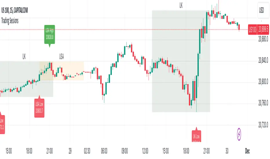
Trading Sessions with Highs and LowsTrading Sessions with Highs and Lows is designed to visually highlight specific trading sessions on the chart, providing traders with key insights into market behavior during these time periods. Here’s a detailed explanation of how the indicator works:
Key Features
1. Session Boxes:
• The indicator plots colored boxes on the chart to represent the price range of defined trading sessions.
• Each box spans the session’s start and end times and encapsulates the high and low prices during that period.
• Two trading sessions are defined by default:
• USA Trading Session: 9:30 AM - 4:00 PM (New York Time).
• UK Trading Session: 8:00 AM - 4:30 PM (London Time).
2. Session Labels:
• The name of the session (e.g., “USA” or “UK”) is displayed above the session box for clear identification.
3. High and Low Markers:
• Markers are added to the chart at the session’s high and low points:
• High Marker: A green label indicating the session high.
• Low Marker: A red label indicating the session low.
4. Dynamic Reset:
• After the session ends, the session high and low values are reset to na to prepare for the next trading day.
5. Customizable Background Colors:
• Each session’s box has a distinct, semi-transparent background color for better visual separation.
How It Works
1. Core Functionality:
• A function, plot_box, takes the session name, start time, end time, and background color as input.
• It calculates whether the current time is within the session.
• During the session:
• It tracks the session’s highest and lowest prices.
• It identifies the bars where the high and low occurred.
• At the session’s end:
• It plots a box on the chart covering the session’s time and price range.
• Labels are created for the session name and its high/low points.
2. Session Timing:
• Timestamps for the USA and UK trading sessions are calculated using the timestamp function with respective time zones.
3. Visual Elements:
• The box.new function draws the session boxes on the chart.
• The label.new function creates session name and high/low labels.
Usage
• Overlay Mode: The indicator is applied directly on the price chart (overlay=true), making it easy to visualize session-specific price behavior.
• Trading Strategy:
• Identify session-specific support and resistance levels.
• Observe price action trends during key trading periods.
• Align trading decisions with session dynamics.
Customization
While the indicator is preset for the USA and UK trading sessions, it can be easily modified:
1. Add/Remove Sessions: Define additional sessions by providing their start and end times.
2. Change Colors: Update the background_color in the plot_box calls to use different colors for sessions.
3. Adjust Time Zones: Replace the current time zones with others relevant to your trading style.
Visualization Example
• USA Session:
• Time: 9:30 AM - 4:00 PM (New York Time).
• Box Color: Semi-transparent orange.
• UK Session:
• Time: 8:00 AM - 4:30 PM (London Time).
• Box Color: Semi-transparent green.
Why Use This Indicator?
1. Market Awareness: Easily spot price behavior during high-liquidity trading periods.
2. Trend Analysis: Analyze how sessions overlap or affect each other.
3. Session Boundaries: Use session high/low levels as dynamic support and resistance zones.
This indicator is an essential tool for intraday and swing traders who want to align their strategies with key market timings.
Search in scripts for "30年国债收益率"
DB369 - Directional Bias 369
DB369 - Directional Bias 369 Indicator
The **DB369** indicator helps traders identify key market levels and trends by combining multiple timeframes' price action analysis. It highlights important **pivot points** on the chart and provides visual cues to help you make more informed buy and sell decisions based on the overall market direction.
Key Features
1. Pivot Points Across Multiple Timeframes**:
- The indicator calculates and displays pivot points for the **Monthly**, **Weekly**, **Daily**, **4-Hour**, and **1-Hour** timeframes (or 30-minute equivalent if desired). These pivots represent significant price levels where the market may retest.
2. **Trend Detection**:
- The indicator evaluates the relationship between the current price and the pivot point for each timeframe. Based on this comparison, it classifies the market as **Bullish**, **Bearish**, or **Neutral** on each timeframe.
3. **Pivot Lines**:
- Horizontal lines are drawn to mark the key pivot points for each selected timeframe. These lines extend into the future and adjust dynamically as the market moves in real time.
- **Customizable**: You can choose which timeframes to display pivot points by enabling/disabling them in the settings.
4. **Trend Table**:
- A **table** is displayed at the top-right of the chart to show the trend for the **Daily**, **4-Hour**, and **30-Minute** timeframes. It provides an easy-to-read view of the trend direction across these timeframes.
5. **Buy/Sell Arrows**:
- **Buy Arrow**: A green arrow will appear when the **Daily**, **4-Hour**, and **30-Minute** trends are all **Bullish** (aligned in the same direction).
- **Sell Arrow**: A red arrow will appear when all three timeframes show a **Bearish** trend.
- These arrows appear only once per alignment change and can be enabled or disabled for alerts. This helps avoid clutter on the chart and ensures that you only see a signal when the alignment occurs or changes.
### **How to Use the DB369 Indicator**:
1. **Pivot Points**:
- The pivot points represent significant price levels where the market might retest in the future. For instance:
- **Bullish Market**: If the price is above the pivot point, the market is considered bullish.
- **Bearish Market**: If the price is below the pivot point, the market is considered bearish.
- **Neutral Market**: When the price is near the pivot point, the market is neither strongly bullish nor bearish.
2. **Trend Alignment**:
- When the **Daily**, **4-Hour**, and **30-Minute** timeframes all show the same trend direction (either **Bullish** or **Bearish**), this alignment signifies a stronger trend.
- You will receive a **Buy Arrow** when all three timeframes are aligned bullish, and a **Sell Arrow** when they are aligned bearish.
- These arrows are displayed at the point when the alignment is first detected and can also trigger **alerts**.
3. **Alerts**:
- You can choose to enable alerts for when a **Buy** or **Sell** arrow appears on the chart. This allows you to be notified in real-time when the alignment conditions are met.
4. **Using the Pivot Points for Entry**:
- **Buy Trade**: Look for a buy trade when the price is near the **pivot line** of the higher timeframes, particularly when the trend across all three timeframes is **Bullish**.
- **Sell Trade**: Similarly, look for a sell trade when the price is near a **pivot line** and the trend is **Bearish**.
5. **Customization**:
- You can customize which timeframes' pivots are shown on the chart by toggling the visibility of the **Monthly**, **Weekly**, **Daily**, **4-Hour**, and **1-Hour** pivots in the settings.
- The indicator automatically adjusts the pivot levels in real-time as the market progresses.
**Important Notes**:
- This indicator does not guarantee successful trades; it is intended to assist in identifying potential trade opportunities based on the alignment of higher timeframe trends.
- Always combine the information from the DB369 indicator with other technical analysis tools and risk management strategies to ensure more accurate trade decisions.

Flashtrader´s Statistical BandwidthsThe vast majority of traders exclusively concern
themselves with trend-following in all its facets. Scoring
points with trends on a regular basis is a difficult task
since prices do not constantly move in one direction
or another. In the case of the DAX future, for example,
only about 30 per cent of all trading days in a year are
trend days. And of these, there are x percent long ones
and x per cent short ones. Catching the very days when
prices rise or fall from the opening to the close is a major
challenge for a trader who also needs to have previously
recognised the corresponding direction.
However, there are also other ways of profit-taking
every day – for example, by using the mean reversion
strategy. The idea behind this is the fact that prices reach
a high and a low every day – but very rarely close at the
high or the low. This means that prices always move
away from these extreme points and the closing price is
somewhere in between. A profitable trading strategy can
be developed out of this.
But how can you know where the high and the low
will be tomorrow? Is it possible for you to know this in
advance? No – because no one can predict the future. Or
can they? At least it can be statistically determined how
high or low prices could go tomorrow. There is a high
degree of probability that one of the two possibilities
will materialise. It will then be necessary to act.
Calculation
Classic pivot points for the following day are calculated
from the high, low and closing price. But does it really
make sense to use such a mix? I don’t think so and
use a different calculation for this strategy. In a first step,
only the differences between the start and the high or low
are calculated on a daily basis. To avoid being dependent
on individual days and outliers, it is advisable to calculate,
in a second step, the average of these differences over
the past five days. Finally, this average will then be added
at the opening price of the current trading day for the
upper statistical bandwidth and subtracted for the lower
bandwidth.
upper bandwidth = oSTB (violet dashed line in the chart)
lower bandwidth = uSTB (violet dashedline in the chart)
The second interesting question is, if the previous day's high has been exceeded, how much further can the price rise from a mathematical/statistical point of view?
These calculated previous day highs expansions are shown as red dashed lines
Previous day's high expansion = VTHA
Previous day's low expansion = VTTA
For further orientation, the previous day's high (VTH) and the previous day's low (VTT) are shown in light blue dashed lines
And as a supplement, the previous day's close in the DAX Future at 10:00 p.m. VTSA in violet solid lines and the previous day's close in the cash register at 5:30 p.m. VTSN in yellow solid lines
Reaching the calculated extreme values does not mean that the trend has to change immediately, but there is at least temporary exhaustion potential with which you can earn a few points every day in the area of scalping.
Example for cheap entry long:
Example for cheap entry short:
Deutsch:
Die Masse der Trader beschäftigt sich ausschließlich mit Trendfolge in all ihren Facetten. Mit Trends regelmäßig zu punkten ist ein schwieriges Unterfangen, da die Kurse nicht ständig in die eine oder andere Richtung laufen. Beim DAX-Future zum Beispiel sind von allen Börsentagen im Jahr lediglich zirka 30 Prozent Trendtage. Davon sind dann auch noch x Prozent Long und x Prozent Short. Hier genau die Tage abzupassen, an denen die Kurse von Börsenbeginn bis zum Schluss steigen beziehungsweise fallen, ist eine große Herausforderung – wobei der Trader zuvor noch die entsprechende Richtung erkannt haben muss. Es gibt jedoch auch noch andere Methoden täglich Gewinne mitzunehmen, zum Beispiel mit der Mean-Reversion-Strategie (Mittelwertumkehr).
Hintergrund ist die Tatsache, dass die Kurse jeden Tag ein Hoch und ein Tief erreichen – aber sehr selten am Hoch oder am Tief schließen. Das bedeutet, dass die Preise sich immer wie der von diesen Extrempunkten wegbewegen und der Schlusskurs irgendwo dazwischen liegt. Hieraus lässt sich eine profitable Handelsstrategie entwickeln. Aber woher kannst Du wissen, wo morgen das Hoch und das Tief sein wird? Kannst Du das vorher schon wissen? Nein – denn niemand kann die Zukunft vorhersagen. Oder doch? Statistisch lässt sich zumindest bestimmen, wie hoch und wie tief die Kurse morgen steigen oder fallen könnten. Eine Seite wird mit sehr hoher Wahrscheinlichkeit ein treffen. Dann gilt es zu handeln.
Berechnung Klassischer Pivot-Punkte für den folgenden Tag werden aus Hoch, Tief und Schlusskurs berechnet. Aber ist es wirklich sinnvoll, einen solchen Mix zu verwenden? Ich finde das nicht und verwenden für diese Strategie eine andere Berechnung. Im ersten Schritt werden täglich die Differenzen nur vom Start bis zum Hoch beziehungsweise Tief errechnet. Um nicht von einzelnen Tagen und Ausreißern abhängig zu sein, empfiehlt es sich, in einem zweiten Schritt den Durchschnitt dieser Differenzen über die letzten fünf Tage zu errechnen. Zuletzt wird dann dieser Durchschnitt zum Eröffnungskurs des aktuellen Handelstages für die obere statistische Bandbreite addiert und für die untere Bandbreite subtrahiert.
Obere statistische Bandbreite = oSTB (violette gestrichelte Linie im Chart)
Untere statistische Bandbreite = uSTB (violette gestrichelte Linie im Chart)
Die zweite interessante Frage ist, wenn das Vortageshoch überschritten wurde, wie weit kann der Kurs dann noch steigen aus mathematisch/statistischer Sicht?
Diese berechneten Vortagesextremausdehnungen sind als rote gestrichelte Linien dargestellt
Vortageshochausdehnung = VTHA
Vortagestiefausdehnung = VTTA
Für die weitere Orientierung sind die Vortageshochs (VTH) und die Vortagestiefs (VTT) als hellblaue gestrichelte Linien abgebildet.
Als Ergänzung wird noch der Vortages Schluss im Dax Future um 22:00 Uhr VTSA mit einer violetten durchgezogenen Linie und der Kassamarktschluss um 17:30 Uhr mit einer gelben durchgezogenen Linie gezeigt.
Das Erreichen der berechneten Extremwerte bedeutet nicht, das der Trend sofort drehen muss, aber es sind zumindest temporäre Erschöpfungspotentiale mit denen sich im Bereich scalping täglich einige Punkte verdienen lassen.
Beispiel für günstigen Einstieg Long:
Beispiel für günstigen Einstieg Short:

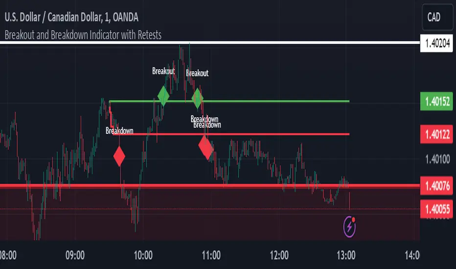
Breakout and Breakdown Indicator with RetestsThis indicator is designed to help traders identify high-probability breakout and breakdown points based on the first 5 minutes of market activity (9:30 am to 9:35 am). It works effectively on both the 1-minute and 5-minute timeframes, making it ideal for day traders and scalpers.
This indicator is a better indicator of my previous 5-Minute Opening Range Breakout indicator.
Key Features:
Dynamic Support and Resistance Lines: Automatically plots the highest and lowest price levels from 9:30 am to 9:35 am, providing essential support and resistance zones.
Breakout/Breakdown Detection: Identifies and marks successful breakout and breakdown points only after a confirmed retest, ensuring more accurate signals.
Visual Markers: Uses customizable green diamonds for successful breakouts and red diamonds for successful breakdowns, allowing easy identification on the chart.
Customization Options:
Change Colors: You can personalize the color of the breakout and breakdown markers, the label text, and the lines drawn from the 9:30 am to 9:35 am window.
Adapt to Your Chart: Adjust the indicator to match your preferred charting theme, ensuring it blends seamlessly with your trading setup.
How It Works:
Plots Key Levels: Identifies the highest and lowest prices during the first 5 minutes of trading (9:30 am to 9:35 am) and plots them on the chart.
Monitors Retests: Waits for a retest of these levels before confirming a breakout or breakdown.
Labels Breakouts/Breakdowns: After a retest, successful breakouts are marked with green diamonds and "Breakout" text, while breakdowns are marked with red diamonds and "Breakdown" text.
Why Use This Indicator?
Avoid False Signals: The retest requirement helps filter out false breakouts and breakdowns, offering more reliable trading signals.
Works Across Timeframes: Suitable for both 1-minute and 5-minute charts, allowing flexibility for different trading styles.
Some what Customizable: Adjust colors to fit your charting preferences and enhance visual clarity.
Recommended Use: Combine this indicator with other technical analysis tools, such as volume, candlestick patterns, or moving averages, for more informed trading decisions.
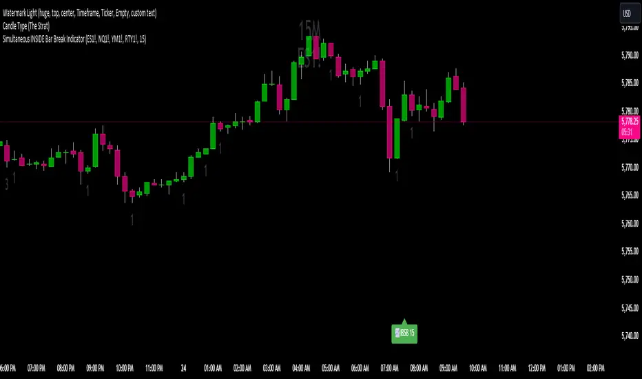
Simultaneous INSIDE Bar Break IndicatorSimultaneous Inside Bar Break Indicator (SIBBI) for The Strat Community
Overview:
The Simultaneous Inside Bar Break Indicator (SIBBI) is designed to help traders using The Strat methodology identify one of the most powerful breakout patterns: the Simultaneous Inside Bar Break across multiple symbols. This indicator detects when all four user-selected symbols form inside bars on the previous candle and then break those inside bars in the same direction (either bullish or bearish) on the current candle.
Inside bars represent consolidation periods where price action does not break the high or low of the previous candle. When a simultaneous break occurs across multiple symbols, this often signals a strong move in the market, making this a key actionable signal in The Strat trading strategy.
Key Features:
Multi-Symbol Analysis: You can track up to four different symbols simultaneously. By default, the indicator comes with SPY, QQQ, IWM, and DIA, but you can modify these to track any other assets or symbols.
Inside Bar Detection: The indicator checks whether all four symbols have inside bars on the previous candle. It only triggers when all symbols meet this condition, making it a highly specific and reliable signal.
Simultaneous Break Detection: Once all symbols have inside bars, the indicator waits for a breakout in the same direction across all four symbols. A simultaneous bullish break (prices breaking above the previous candle’s high) triggers a green label, while a simultaneous bearish break (prices breaking below the previous candle’s low) triggers a red label.
Dynamic Label Timeframe: The indicator dynamically adjusts the timeframe in the label based on the user’s selected timeframe. This allows traders to know precisely which timeframe the break is occurring on. If the user selects "Chart Timeframe," the indicator will evolve with the current chart's timeframe, making it more versatile.
Timeframe Flexibility: The indicator can be set to analyze any timeframe—15-minute, 30-minute, 60-minute, daily, weekly, and so on. It only works for the specific timeframe you set it to in the settings. If set to "Chart Timeframe," the label will adapt dynamically based on the timeframe you are currently viewing.
Customizable Labels: The user can choose the size of the labels (tiny, small, or normal), ensuring that the visual output is tailored to individual preferences and chart layouts.
Best Use Case:
The Simultaneous Inside Bar Break Indicator is particularly powerful when applied to multiple timeframes. Here’s how to use it for maximum impact:
Multi-Timeframe Setup: Set the indicator on various timeframes (e.g., 15-minute, 30-minute, 60-minute, and daily) across multiple charts. This allows you to monitor different timeframes and identify when lower timeframe breaks trigger potential moves on higher timeframes.
Anticipating Strong Moves: When a simultaneous inside bar break occurs on one timeframe (e.g., 30-minute), keep an eye on the higher timeframes (e.g., 60-minute or daily) to see if those timeframes also break. This stacking of inside bar breaks can signal powerful market moves.
Higher Conviction Signals: The indicator is designed to provide high-conviction signals. Since it requires all four symbols to break in the same direction simultaneously, it reduces false signals and focuses on higher probability setups, which is crucial for traders using The Strat to time their trades effectively.
How the Indicator Works:
Inside Bar Formation: The indicator first checks that all four selected symbols had inside bars in the previous bar (i.e., the current high and low are contained within the previous bar’s high and low).
Simultaneous Break Detection: After detecting inside bars, the indicator checks if all four symbols break out in the same direction—bullish (breaking above the previous bar’s high) or bearish (breaking below the previous bar’s low).
Label Display: When a simultaneous inside bar break occurs, a label is plotted on the chart—either green for a bullish break (below the candle) or red for a bearish break (above the candle). The label will display the timeframe you set in the settings (e.g., "IBSB 60" for a 60-minute break).
Chart Timeframe Option: If you prefer, you can set the indicator to evolve with the chart’s current timeframe. In this mode, the label will not show a specific timeframe but will still display the simultaneous inside bar break when it occurs.
Recommendations for Usage:
Focus on Multiple Timeframes: The Strat methodology is all about understanding the relationship between different timeframes. Use this indicator on multiple timeframes to get a better picture of potential moves.
Pair with Other Strat Techniques: This indicator is most powerful when combined with other Strat tools, such as broadening formations, timeframe continuity, and actionable signals (e.g., 2-2 reversals). The simultaneous inside bar break can help confirm or invalidate other signals.
Customize Symbols and Timeframes: Although the default symbols are SPY, QQQ, IWM, and DIA, feel free to replace them with symbols more relevant to your trading. This indicator works well across equities, indices, futures, and forex pairs.
How to Set It Up:
Select Symbols: Choose four symbols that you want to track. These can be index ETFs (like SPY and QQQ), individual stocks, or any other tradable instruments.
Set Timeframe: In the indicator’s settings, choose a specific timeframe (e.g., 15-minute, 30-minute, daily). The label will reflect the selected timeframe, making it clear which time-based break you are seeing.
Optional - Chart Timeframe Mode: If you want the indicator to adapt to the chart’s current timeframe, select the "Chart Timeframe" option in the settings. The indicator will plot the breaks without showing a specific timeframe in the label.
Customize Label Size: Depending on your chart layout and personal preference, you can adjust the size of the labels (tiny, small, or normal) in the settings.
Conclusion:
The Simultaneous Inside Bar Break Indicator is a powerful tool for traders using The Strat methodology, offering a highly specific and reliable signal that can indicate potential large market moves. By monitoring multiple symbols and timeframes, you can gain deeper insight into the market's behavior and act with greater confidence. This indicator is ideal for traders looking to catch high-conviction moves and align their trades with broader market continuity.
Note: The indicator works best when paired with multi-timeframe analysis, allowing you to see how breaks on lower timeframes might influence larger trends. For traders who prefer simplicity, setting it to the "Chart Timeframe" mode offers flexibility while maintaining the core benefits of this indicator.
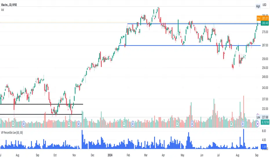
Volume-Price PercentileDescription:
The "Volume-Price Percentile Live" indicator is designed to provide real-time analysis of the relationship between volume percentiles and price percentiles on any given timeframe. This tool helps traders assess market activity by comparing how current volume levels rank relative to historical volume data and how current price movements (specifically high-low ranges) rank relative to historical price data. The indicator visualizes the ratio of volume percentile to price percentile as a histogram, allowing traders to gauge the relative strength of volume against price movements in real time.
Functionality:
Volume Percentile: Calculates the percentile rank of the current volume within a user-defined rolling period (default is 30 bars). This percentile indicates where the current volume stands in comparison to historical volumes over the specified period.
Price Percentile: Calculates the percentile rank of the current candle's high-low difference within a user-defined rolling period (default is 30 bars). This percentile reflects the current price movement's strength relative to past movements over the specified period.
Percentile Ratio (VP Ratio): The indicator plots the ratio of the volume percentile to the price percentile. This ratio helps identify periods when volume is significantly higher or lower relative to price movement, providing insights into potential market imbalances or strength.
Real-Time Data: By fetching data from a lower timeframe (e.g., 1-minute), the indicator updates continuously within the current timeframe, offering live, intra-candle updates. This ensures that traders can see the histogram change in real-time as new data becomes available, without waiting for the current candle to close.
How to Use:
Adding the Indicator: To use this indicator, add it to your chart on TradingView by selecting it from the Indicators list once it is published publicly.
Setting Parameters:
Volume Period Length: This input sets the rolling window length for calculating the volume percentile (default is 30). You can adjust it based on the desired sensitivity or historical period relevance.
Candle Period Length: This input sets the rolling window length for calculating the price percentile based on the high-low difference of candles (default is 30). Adjust this to match your trading style or analysis period.
Interpreting the Histogram:
The histogram represents the volume percentile divided by the price percentile.
Above 1: A value greater than 1 indicates that volume is relatively strong compared to price movement, which may suggest high activity or potential accumulation/distribution phases.
Below 1: A value less than 1 suggests that price movement is relatively stronger than volume, indicating potential weakness in volume relative to price moves.
Near 1: Values close to 1 suggest a balanced relationship between volume and price movement.
Application: Use this indicator to identify potential breakout or breakdown scenarios, assess the strength of price movements, and confirm trends. When volume percentile consistently leads price percentile, it might signal sustained interest and support for the current price trend. Conversely, if volume percentile lags significantly, it might warn of potential trend weakness.
Best Practices:
Multiple Timeframe Analysis: While the indicator provides real-time updates on any timeframe, consider using it alongside higher timeframe analysis to confirm trends and volume behavior across different periods.
Customization: Adjust the period lengths based on the asset’s typical volume and price behavior, as well as your trading strategy (e.g., short-term scalping vs. long-term trend following).
Complement with Other Indicators: Use this indicator in conjunction with other volume-based tools, trend indicators, or momentum oscillators to gain a comprehensive view of market dynamics.
1 (or) 5-Minute Scalping Strategy - KGP1-Minute Scalping Strategy - KGP
Overview: This indicator is designed for short-term traders who engage in 1 (or) 5-minute scalping. It combines several technical analysis tools to provide buy and sell signals, helping traders make informed decisions quickly.
Key Features:
VWAP (Volume Weighted Average Price):
Purpose: VWAP provides the average price a security has traded at throughout the day, based on both volume and price.
Usage: Helps identify the overall trend and potential entry points. When the price is above VWAP, it indicates a bullish trend; when below, it indicates a bearish trend.
RSI (Relative Strength Index):
Purpose: RSI measures the speed and change of price movements, indicating overbought or oversold conditions.
Usage: The RSI values between 30 and 70 are used to filter trades. A value above 70 indicates overbought conditions, while below 30 indicates oversold conditions.
Custom OBV (On Balance Volume):
Purpose: OBV uses volume flow to predict changes in stock price.
Usage: Helps confirm the strength of a trend. Increasing OBV indicates accumulation (buying pressure), while decreasing OBV indicates distribution (selling pressure).
Multi-Timeframe Analysis:
Purpose: Confirms signals by analyzing RSI on a higher timeframe (5-minute chart).
Usage: Ensures that signals on the 1-minute chart align with the broader trend on the 5-minute chart, reducing false signals.
Signals:
Buy Signal:
Triggered when the price crosses above the VWAP, and the RSI is between 50 and 70 on both the 1-minute and 5-minute charts.
Visual Cue: A green “BUY” label appears below the bar.'
Sell Signal:
Triggered when the price crosses below the VWAP, and the RSI is between 30 and 50 on both the 1-minute and 5-minute charts.
Visual Cue: A red “SELL” label appears above the bar.
Alerts:
Buy Alert: Notifies you when a buy signal is detected.
Sell Alert: Notifies you when a sell signal is detected.
Additional Visuals:
VWAP Line: Plotted in blue to show the average price based on volume.
OBV Line: Plotted in purple to indicate volume flow.
RSI Line: Plotted in orange with horizontal lines at 70 (overbought) and 30 (oversold) levels.

Multi-Length RSI **Multi-Length RSI Indicator**
This script creates a custom Relative Strength Index (RSI) indicator with the ability to plot three different RSI lengths on the same chart, allowing traders to analyze momentum across various timeframes simultaneously. The script also includes features to enhance visual clarity and usability.
**Key Features:**
1. **Customizable RSI Lengths:**
- The script allows you to input and customize three different RSI lengths (7, 14, and 28 by default) via user inputs. This flexibility enables you to track short-term, medium-term, and long-term momentum in the market.
2. **Dynamic Colour Coding:**
- The RSI lines are color-coded based on their current value:
- **Above 70 (Overbought)**: The line turns red.
- **Below 30 (Oversold)**: The line turns green.
- **Between 30 and 70**: The line retains its user-defined colour (blue, yellow, orange by default).
- This dynamic colouring helps to quickly identify overbought and oversold conditions.
3. **Adjustable Line Widths and Colours:**
- Users can customize the colour and thickness of each RSI line, allowing for a personalized visual experience that fits different trading strategies.
4. **Overbought, Oversold, and Midline Levels:**
- The script includes static horizontal lines at the 70 (Overbought) and 30 (Oversold) levels, with a red and green colour, respectively.
- A midline at the 50 level is also included in gray and dashed, helping to visualize the neutral zone.
5. **Dynamic RSI Value Labels:**
- The current values of each RSI line are displayed directly on the chart as labels at the most recent bar, with colours matching their corresponding lines. This feature provides an immediate reference to the exact RSI values without the need to hover or look at the data window.
6. **Alerts for Crosses:**
- The script includes built-in alert conditions for when any of the RSI values cross above the overbought level (70) or below the oversold level (30). These alerts can be configured to notify you in real-time when significant momentum shifts occur.
**How to Use:**
1. **Customization**:
- Input your preferred RSI lengths, colours, and line widths through the script’s settings menu.
2. **Visual Analysis**:
- The indicator plots all three RSI values on a separate pane below the price chart. Use the color-coded lines and levels to quickly identify overbought, oversold, and neutral conditions across multiple timeframes.
3. **Set Alerts**:
- You can configure alerts based on the built-in alert conditions to get notified when the RSI crosses critical levels.
**Ideal For:**
- **Traders looking to analyze momentum across multiple timeframes**: The ability to view short-term, medium-term, and long-term RSIs simultaneously offers a comprehensive view of market strength.
- **Those who prefer visual clarity**: The dynamic colouring, clear labels, and customizable settings make it easy to interpret RSI data at a glance.
- **Traders who rely on alerts**: The built-in alert system allows for proactive trading based on significant RSI level crossings.
---
This script is a powerful tool for any trader looking to leverage RSI analysis across multiple timeframes, offering both customization and clarity in a single indicator.
MACD with 1D Stochastic Confirmation Reversal StrategyOverview
The MACD with 1D Stochastic Confirmation Reversal Strategy utilizes MACD indicator in conjunction with 1 day timeframe Stochastic indicators to obtain the high probability short-term trend reversal signals. The main idea is to wait until MACD line crosses up it’s signal line, at the same time Stochastic indicator on 1D time frame shall show the uptrend (will be discussed in methodology) and not to be in the oversold territory. Strategy works on time frames from 30 min to 4 hours and opens only long trades.
Unique Features
Dynamic stop-loss system: Instead of fixed stop-loss level strategy utilizes average true range (ATR) multiplied by user given number subtracted from the position entry price as a dynamic stop loss level.
Configurable Trading Periods: Users can tailor the strategy to specific market windows, adapting to different market conditions.
Higher time frame confirmation: Strategy utilizes 1D Stochastic to establish the major trend and confirm the local reversals with the higher probability.
Trailing take profit level: After reaching the trailing profit activation level scrip activate the trailing of long trade using EMA. More information in methodology.
Methodology
The strategy opens long trade when the following price met the conditions:
MACD line of MACD indicator shall cross over the signal line of MACD indicator.
1D time frame Stochastic’s K line shall be above the D line.
1D time frame Stochastic’s K line value shall be below 80 (not overbought)
When long trade is executed, strategy set the stop-loss level at the price ATR multiplied by user-given value below the entry price. This level is recalculated on every next candle close, adjusting to the current market volatility.
At the same time strategy set up the trailing stop validation level. When the price crosses the level equals entry price plus ATR multiplied by user-given value script starts to trail the price with EMA. If price closes below EMA long trade is closed. When the trailing starts, script prints the label “Trailing Activated”.
Strategy settings
In the inputs window user can setup the following strategy settings:
ATR Stop Loss (by default = 3.25, value multiplied by ATR to be subtracted from position entry price to setup stop loss)
ATR Trailing Profit Activation Level (by default = 4.25, value multiplied by ATR to be added to position entry price to setup trailing profit activation level)
Trailing EMA Length (by default = 20, period for EMA, when price reached trailing profit activation level EMA will stop out of position if price closes below it)
User can choose the optimal parameters during backtesting on certain price chart, in our example we use default settings.
Justification of Methodology
This strategy leverages 2 time frames analysis to have the high probability reversal setups on lower time frame in the direction of the 1D time frame trend. That’s why it’s recommended to use this strategy on 30 min – 4 hours time frames.
To have an approximation of 1D time frame trend strategy utilizes classical Stochastic indicator. The Stochastic Indicator is a momentum oscillator that compares a security's closing price to its price range over a specific period. It's used to identify overbought and oversold conditions. The indicator ranges from 0 to 100, with readings above 80 indicating overbought conditions and readings below 20 indicating oversold conditions.
It consists of two lines:
%K: The main line, calculated using the formula (CurrentClose−LowestLow)/(HighestHigh−LowestLow)×100 . Highest and lowest price taken for 14 periods.
%D: A smoothed moving average of %K, often used as a signal line.
Strategy logic assumes that on 1D time frame it’s uptrend in %K line is above the %D line. Moreover, we can consider long trade only in %K line is below 80. It means that in overbought state the long trade will not be opened due to higher probability of pullback or even major trend reversal. If these conditions are met we are going to our working (lower) time frame.
On the chosen time frame, we remind you that for correct work of this strategy you shall use 30min – 4h time frames, MACD line shall cross over it’s signal line. The MACD (Moving Average Convergence Divergence) is a popular momentum and trend-following indicator used in technical analysis. It helps traders identify changes in the strength, direction, momentum, and duration of a trend in a stock's price.
The MACD consists of three components:
MACD Line: This is the difference between a short-term Exponential Moving Average (EMA) and a long-term EMA, typically calculated as: MACD Line=12-period EMA−26-period
Signal Line: This is a 9-period EMA of the MACD Line, which helps to identify buy or sell signals. When the MACD Line crosses above the Signal Line, it can be a bullish signal (suggesting a buy); when it crosses below, it can be a bearish signal (suggesting a sell).
Histogram: The histogram shows the difference between the MACD Line and the Signal Line, visually representing the momentum of the trend. Positive histogram values indicate increasing bullish momentum, while negative values indicate increasing bearish momentum.
In our script we are interested in only MACD and signal lines. When MACD line crosses signal line there is a high chance that short-term trend reversed to the upside. We use this strategy on 45 min time frame.
ATR is used to adjust the strategy risk management to the current market volatility. If volatility is low, we don’t need the large stop loss to understand the there is a high probability that we made a mistake opening the trade. User can setup the settings ATR Stop Loss and ATR Trailing Profit Activation Level to realize his own risk to reward preferences, but the unique feature of a strategy is that after reaching trailing profit activation level strategy is trying to follow the trend until it is likely to be finished instead of using fixed risk management settings. It allows sometimes to be involved in the large movements.
Backtest Results
Operating window: Date range of backtests is 2023.01.01 - 2024.08.01. It is chosen to let the strategy to close all opened positions.
Commission and Slippage: Includes a standard Binance commission of 0.1% and accounts for possible slippage over 5 ticks.
Initial capital: 10000 USDT
Percent of capital used in every trade: 30%
Maximum Single Position Loss: -4.79%
Maximum Single Profit: +20.14%
Net Profit: +2361.33 USDT (+44.72%)
Total Trades: 123 (44.72% win rate)
Profit Factor: 1.623
Maximum Accumulated Loss: 695.80 USDT (-5.48%)
Average Profit per Trade: 19.20 USDT (+0.59%)
Average Trade Duration: 30 hours
These results are obtained with realistic parameters representing trading conditions observed at major exchanges such as Binance and with realistic trading portfolio usage parameters.
How to Use
Add the script to favorites for easy access.
Apply to the desired timeframe between 30 min and 4 hours and chart (optimal performance observed on 45 min BTC/USDT).
Configure settings using the dropdown choice list in the built-in menu.
Set up alerts to automate strategy positions through web hook with the text: {{strategy.order.alert_message}}
Disclaimer:
Educational and informational tool reflecting Skyrex commitment to informed trading. Past performance does not guarantee future results. Test strategies in a simulated environment before live implementation

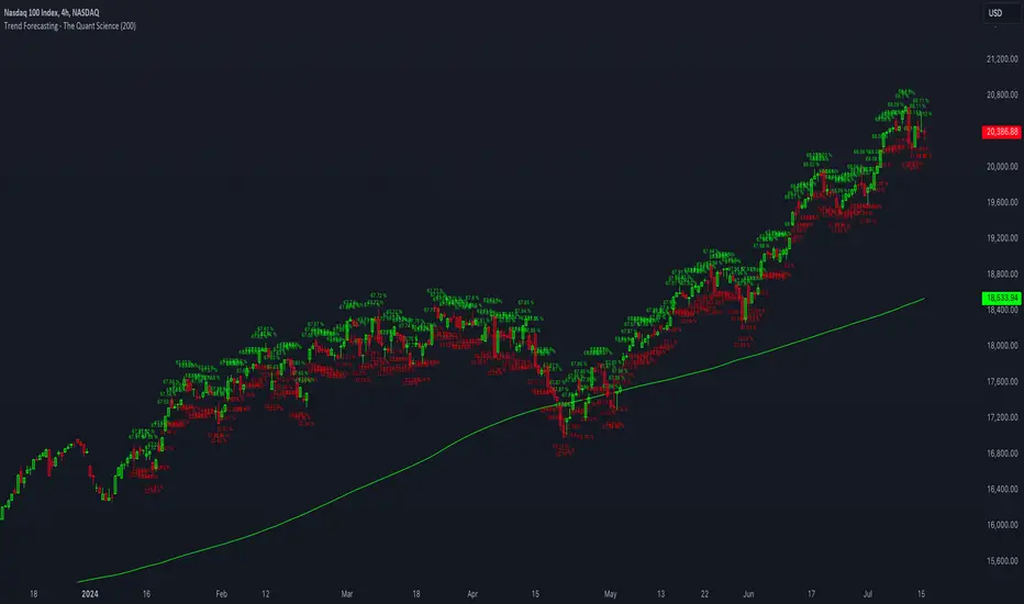
Trend Forecasting - The Quant Science🌏 Trend Forecasting | ENG 🌏
This plug-in acts as a statistical filter, adding new information to your chart that will allow you to quickly verify the direction of a trend and the probability with which the price will be above or below the average in the future, helping you to uncover probable market inefficiencies.
🧠 Model calculation
The model calculates the arithmetic mean in relation to positive and negative events within the available sample for the selected time series. Where a positive event is defined as a closing price greater than the average, and a negative event as a closing price less than the average. Once all events have been calculated, the probabilities are extrapolated by relating each event.
Example
Positive event A: 70
Negative event B: 30
Total events: 100
Probabilities A: (100 / 70) x 100 = 70%
Probabilities B: (100 / 30) x 100 = 30%
Event A has a 70% probability of occurring compared to Event B which has a 30% probability.
🔍 Information Filter
The data on the graph show the future probabilities of prices being above average (default in green) and the probabilities of prices being below average (default in red).
The information that can be quickly retrieved from this indicator is:
1. Trend: Above-average prices together with a constant of data in green greater than 50% + 1 indicate that the observed historical series shows a bullish trend. The probability is correlated proportionally to the value of the data; the higher and increasing the expected value, the greater the observed bullish trend. On the other hand, a below-average price together with a red-coloured data constant show quantitative data regarding the presence of a bearish trend.
2. Future Probability: By analysing the data, it is possible to find the probability with which the price will be above or below the average in the future. In green are classified the probabilities that the price will be higher than the average, in red are classified the probabilities that the price will be lower than the average.
🔫 Operational Filter .
The indicator can be used operationally in the search for investment or trading opportunities given its ability to identify an inefficiency within the observed data sample.
⬆ Bullish forecast
For bullish trades, the inefficiency will appear as a historical series with a bullish trend, with high probability of a bullish trend in the future that is currently below the average.
⬇ Bearish forecast
For short trades, the inefficiency will appear as a historical series with a bearish trend, with a high probability of a bearish trend in the future that is currently above the average.
📚 Settings
Input: via the Input user interface, it is possible to adjust the periods (1 to 500) with which the average is to be calculated. By default the periods are set to 200, which means that the average is calculated by taking the last 200 periods.
Style: via the Style user interface it is possible to adjust the colour and switch a specific output on or off.
🇮🇹Previsione Della Tendenza Futura | ITA 🇮🇹
Questo plug-in funge da filtro statistico, aggiungendo nuove informazioni al tuo grafico che ti permetteranno di verificare rapidamente tendenza di un trend, probabilità con la quale il prezzo si troverà sopra o sotto la media in futuro aiutandoti a scovare probabili inefficienze di mercato.
🧠 Calcolo del modello
Il modello calcola la media aritmetica in relazione con gli eventi positivi e negativi all'intero del campione disponibile per la serie storica selezionata. Dove per evento positivo si intende un prezzo alla chiusura maggiore della media, mentre per evento negativo si intende un prezzo alla chiusura minore della media. Calcolata la totalità degli eventi le probabilità vengono estrapolate rapportando ciascun evento.
Esempio
Evento positivo A: 70
Evento negativo B: 30
Totale eventi : 100
Formula A: (100 / 70) x 100 = 70%
Formula B: (100 / 30) x 100 = 30%
Evento A ha una probabilità del 70% di realizzarsi rispetto all' Evento B che ha una probabilità pari al 30%.
🔍 Filtro informativo
I dati sul grafico mostrano le probabilità future che i prezzi siano sopra la media (di default in verde) e le probabilità che i prezzi siano sotto la media (di default in rosso).
Le informazioni che si possono rapidamente reperire da questo indicatore sono:
1. Trend: I prezzi sopra la media insieme ad una costante di dati in verde maggiori al 50% + 1 indicano che la serie storica osservata presenta un trend rialzista. La probabilità è correlata proporzionalmente al valore del dato; tanto più sarà alto e crescente il valore atteso e maggiore sarà la tendenza rialzista osservata. Viceversa, un prezzo sotto la media insieme ad una costante di dati classificati in colore rosso mostrano dati quantitativi riguardo la presenza di una tendenza ribassista.
2. Probabilità future: analizzando i dati è possibile reperire la probabilità con cui il prezzo si troverà sopra o sotto la media in futuro. In verde vengono classificate le probabilità che il prezzo sarà maggiore alla media, in rosso vengono classificate le probabilità che il prezzo sarà minore della media.
🔫 Filtro operativo
L' indicatore può essere utilizzato a livello operativo nella ricerca di opportunità di investimento o di trading vista la capacità di identificare un inefficienza all'interno del campione di dati osservato.
⬆ Previsione rialzista
Per operatività di tipo rialzista l'inefficienza apparirà come una serie storica a tendenza rialzista, con alte probabilità di tendenza rialzista in futuro che attualmente si trova al di sotto della media.
⬇ Previsione ribassista
Per operatività di tipo short l'inefficienza apparirà come una serie storica a tendenza ribassista, con alte probabilità di tendenza ribassista in futuro che si trova attualmente sopra la media.
📚 Impostazioni
Input: tramite l'interfaccia utente Input è possibile regolare i periodi (da 1 a 500) con cui calcolare la media. Di default i periodi sono impostati sul valore di 200, questo significa che la media viene calcolata prendendo gli ultimi 200 periodi.
Style: tramite l'interfaccia utente Style è possibile regolare il colore e attivare o disattivare un specifico output.
Candle Wick Shadows [UkutaLabs]█ OVERVIEW
The Candle Wick Shadows Indicator identifies untested wicks in real time that occur when there is an imbalance in the number of buyers and sellers at a price-level. This imbalance occurs when a market exchange receives too many of one kind of order, and not enough of its counterpoint.
Candle Wick Shadows is a powerful trading indicator that will automatically identify and label strong ranges on traders’ charts that can be incorporated into a wide variety of different trading strategies.
█ USAGE
The script automatically identifies and measures real-time ranges of imbalance between buying and selling pressure in the market using real-time price-action information. These levels indicate potential Supply and Demand zones which serve to help the trader identify areas where price has changed direction in the past due to an imbalance of buyers and sellers.
The script also allows users to mirror higher time frame Candle Wick Shadows onto lower time frame charts to gain a stronger understanding of key levels on another scale.
█ SETTINGS
Configuration
- Show Labels: Determines whether or not identification labels are drawn on the chart.
- Max CWS Display: Determines the number of Candle Wick Shadows that will be drawn on the chart. This is for each higher timeframe option that is toggled, not the total.
Current Time Frame
-Wick Shadow (On/Off): Determines whether or not wick shadows are drawn from the current time frame chart.
- Bullish Color: Determines the color of bullish wick shadows from the current time frame.
- Bearish Color: Determines the color of bearish wick shadows from the current time frame.
5 Minute (Higher Timeframe)
-Wick Shadow (On/Off): Determines whether or not wick shadows are drawn from the 5 minute time frame chart.
- Bullish Color: Determines the color of bullish wick shadows from the 5 minute time frame.
- Bearish Color: Determines the color of bearish wick shadows from the 5 minute time frame.
15 Minute (Higher Timeframe)
-Wick Shadow (On/Off): Determines whether or not wick shadows are drawn from the 15 minute time frame chart.
- Bullish Color: Determines the color of bullish wick shadows from the 15 minute time frame.
- Bearish Color: Determines the color of bearish wick shadows from the 15 minute time frame.
30 Minute (Higher Timeframe)
-Wick Shadow (On/Off): Determines whether or not wick shadows are drawn from the 30 minute time frame chart.
- Bullish Color: Determines the color of bullish wick shadows from the 30 minute time frame.
- Bearish Color: Determines the color of bearish wick shadows from the 30 minute time frame.
60 Minute (Higher Timeframe)
-Wick Shadow (On/Off): Determines whether or not wick shadows are drawn from the 60 minute time frame chart.
- Bullish Color: Determines the color of bullish wick shadows from the 60 minute time frame.
- Bearish Color: Determines the color of bearish wick shadows from the 60 minute time frame.
240 Minute (Higher Timeframe)
-Wick Shadow (On/Off): Determines whether or not wick shadows are drawn from the 240 minute time frame chart.
- Bullish Color: Determines the color of bullish wick shadows from the 240 minute time frame.
- Bearish Color: Determines the color of bearish wick shadows from the 240 minute time frame.
Daily (Higher Timeframe)
-Wick Shadow (On/Off): Determines whether or not wick shadows are drawn from the daily time frame chart.
- Bullish Color: Determines the color of bullish wick shadows from the daily time frame.
- Bearish Color: Determines the color of bearish wick shadows from the daily time frame.

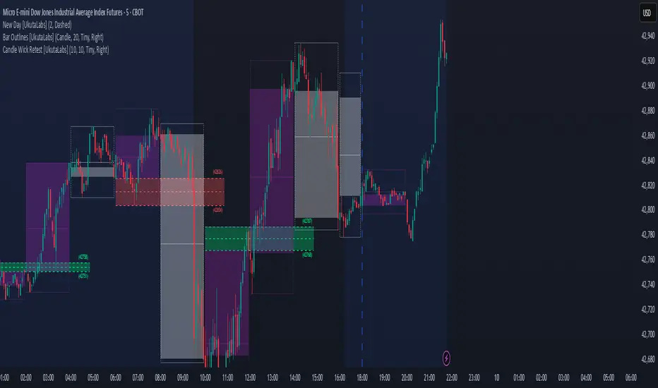
Candle Wick Retest [UkutaLabs]█ OVERVIEW
The Candle Wick Retest Indicator identifies untested wicks in real time that occur when there is an imbalance in the number of buyers and sellers at a price-level. This imbalance occurs when a market exchange receives too many of one kind of order, and not enough of its counterpoint.
Candle Wick Retest is a powerful trading indicator that will automatically identify and label strong ranges on traders’ charts that can be incorporated into a wide variety of different trading strategies.
█ USAGE
The script automatically identifies and measures real-time ranges of imbalance between buying and selling pressure in the market using real-time price-action information. These levels indicate potential Supply and Demand zones which serve to help the trader identify areas where price has changed direction in the past due to an imbalance of buyers and sellers.
The script also allows users to mirror higher time frame Candle Wick Retests onto lower time frame charts to gain a stronger understanding of key levels on another scale.
█ SETTINGS
Configuration
- Show Labels: Determines whether or not identification labels are drawn on the chart.
- Max CW Display: Determines the number of Candle Wick Retests that will be drawn on the chart. This is for each higher timeframe option that is toggled, not the total.
Current Time Frame
- Wick Retest (On/Off): Determines whether wick retests will be drawn from the current time frame chart.
- Wick Retest Bullish Color: Determines the color of bullish wick retests from the current time frame.
- Wick Retest Bearish Color: Determines the color of bearish wick retests from the current time frame.
5 Minute (Higher Timeframe)
- Wick Retest (On/Off): Determines whether wick retests will be drawn from the 5 minute chart.
- Wick Retest Bullish Color: Determines the color of bullish wick retests from the 5 minute time frame.
- Wick Retest Bearish Color: Determines the color of bearish wick retests from the 5 minute time frame.
15 Minute (Higher Timeframe)
- Wick Retest (On/Off): Determines whether wick retests will be drawn from the 15 minute time frame chart.
- Wick Retest Bullish Color: Determines the color of bullish wick retests from the 15 minute time frame.
- Wick Retest Bearish Color: Determines the color of bearish wick retests from the 15 minute time frame.
30 Minute (Higher Timeframe)
- Wick Retest (On/Off): Determines whether wick retests will be drawn from the 30 minute time frame chart.
- Wick Retest Bullish Color: Determines the color of bullish wick retests from the 30 minute time frame.
- Wick Retest Bearish Color: Determines the color of bearish wick retests from the 30 minute time frame.
60 Minute (Higher Timeframe)
- Wick Retest (On/Off): Determines whether wick retests will be drawn from the 60 minute time frame chart.
- Wick Retest Bullish Color: Determines the color of bullish wick retests from the 60 minute time frame.
- Wick Retest Bearish Color: Determines the color of bearish wick retests from the 60 minute time frame.
240 Minute (Higher Timeframe)
- Wick Retest (On/Off): Determines whether wick retests will be drawn from the 240 minute time frame chart.
- Wick Retest Bullish Color: Determines the color of bullish wick retests from the 240 minute time frame.
- Wick Retest Bearish Color: Determines the color of bearish wick retests from the 240 minute time frame.
Daily (Higher Timeframe)
- Wick Retest (On/Off): Determines whether wick retests will be drawn from the daily time frame chart.
- Wick Retest Bullish Color: Determines the color of bullish wick retests from the daily time frame.
- Wick Retest Bearish Color: Determines the color of bearish wick retests from the daily time frame.
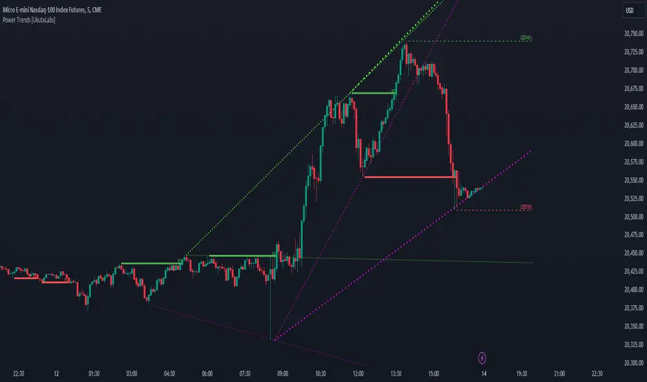
Power Trends [UkutaLabs]█ OVERVIEW
The Power Trends Indicator is a versatile trading toolkit that offers unique insight into key price levels in the market. This script uses currently relevant price-action information to automatically detect pivot levels and use them to create powerful trendlines.
The aim of this script is to improve the trading experience of users by offering a versatile toolkit that can be used in a wide variety of trading strategies to help simplify the complexities of the market.
█ USAGE
The Power Trends Indicator will automatically identify pivot points in real-time using recent price-action information to ensure that all points being identified are relevant. Using these pivot points, the script then draws powerful trend lines that can be used as levels of resistance and support.
To ensure that only the most relevant information is being presented, only the most recent trend lines will be displayed on the user’s charts. As new trend lines are being drawn, older trend lines will become thinner so that traders can identify the most relevant lines at a glance.
The price of the most recent high and low pivot points will also be displayed on the chart and can be used as further levels of resistance and support.
When a recent pivot level is broken, it will be identified as a Break of Structure. This signifies that there may have been a change in market strength.
The Power Trends Indicator also supports multiple time frame mapping, allowing you to mirror the trend lines that would be drawn on higher time frame charts onto lower time frame charts. This feature allows traders to be aware of the market structure of multiple charts at a glance from a single chart.
When mirroring some higher time frame trend lines, lines may appear to not align properly with current time frame bars. This is done intentionally to ensure lines are being drawn accurately to their position on the higher time frame charts.
█ SETTINGS
Current Time Frame
• Display (On/Off): Determines whether or not trend lines are drawn from the current time frame.
• High Color: Determines the color of trend lines drawn on high pivots.
• Low Color: Determines the color of trend lines drawn on low pivots.
5 Minute (Higher Time Frame)
• Display (On/Off): Determines whether or not trend lines are drawn from the 5 minute higher time frame.
• High Color: Determines the color of trend lines drawn on high pivots from the 5 minute higher time frame.
• Low Color: Determines the color of trend lines drawn on low pivots from the 5 minute higher time frame.
15 Minute (Higher Time Frame)
• Display (On/Off): Determines whether or not trend lines are drawn from the 15 minute higher time frame.
• High Color: Determines the color of trend lines drawn on high pivots from the 15 minute higher time frame.
• Low Color: Determines the color of trend lines drawn on low pivots from the 15 minute higher time frame.
30 Minute (Higher Time Frame)
• Display (On/Off): Determines whether or not trend lines are drawn from the 30 minute higher time frame.
• High Color: Determines the color of trend lines drawn on high pivots from the 30 minute higher time frame.
• Low Color: Determines the color of trend lines drawn on low pivots from the 30 minute higher time frame.
60 Minute (Higher Time Frame)
• Display (On/Off): Determines whether or not trend lines are drawn from the 60 minute higher time frame.
• High Color: Determines the color of trend lines drawn on high pivots from the 60 minute higher time frame.
• Low Color: Determines the color of trend lines drawn on low pivots from the 60 minute higher time frame.
240 Minute (Higher Time Frame)
• Display (On/Off): Determines whether or not trend lines are drawn from the 240 minute higher time frame.
• High Color: Determines the color of trend lines drawn on high pivots from the 240 minute higher time frame.
• Low Color: Determines the color of trend lines drawn on low pivots from the 240 minute higher time frame.
Daily (Higher Time Frame)
• Display (On/Off): Determines whether or not trend lines are drawn from the daily time frame.
• High Color: Determines the color of trend lines drawn on high pivots from the daily higher time frame.
• Low Color: Determines the color of trend lines drawn on low pivots from the daily higher time frame.
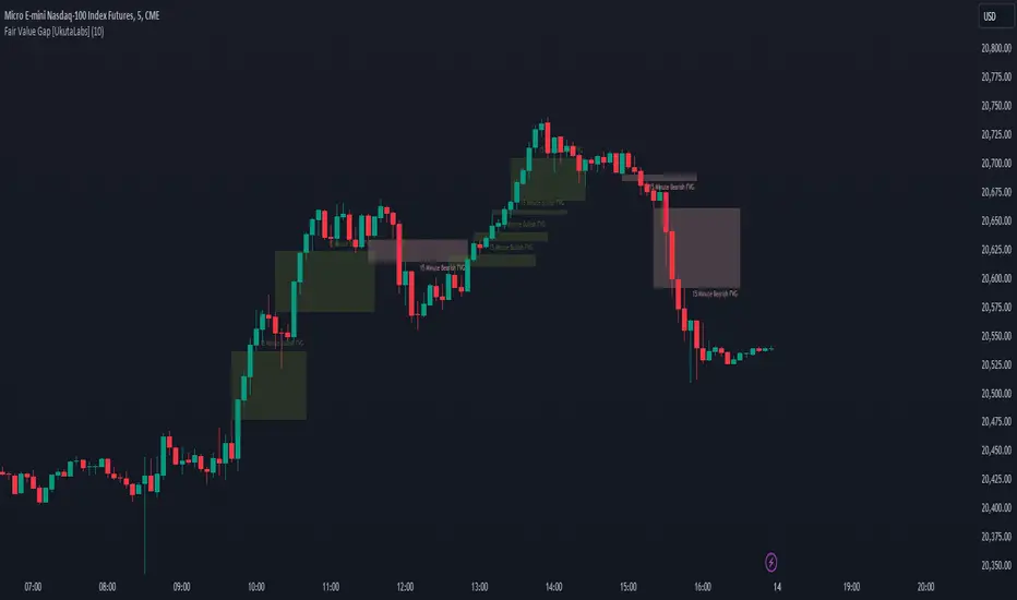
Fair Value Gap [UkutaLabs]█ OVERVIEW
Fair Value Gaps are price jumps caused by the imbalance buying and selling pressures in trading and are most commonly used amongst price action traders. Fair Value Gaps are formed via a three-candle sequence in which a large candle’s neighbouring candles’ upper and lower wicks do not fully overlap the large candle.
The Fair Value Gaps Indicator also supports Multi Time Frame Plotting, allowing you to plot the Fair Value Gaps from higher time frames onto lower time frame charts.
The Fair Value Gaps Indicator is a powerful trading toolkit that provides users with more information than they would typically have available to them by allowing them to configure several charts worth of information onto one single chart.
█ USAGE
The script automatically identifies imbalances between buying and selling pressure in the market in real time, offering traders valuable insight into current market sentiment. These gaps are considered to be levels where the supply and demand of a commodity are imbalanced, and the price tends to return to fill these gaps (But are not guaranteed to).
The Fair Value Gaps Indicator also allows gaps from higher time frames to be drawn on lower time frame charts, providing traders with more information than they would typically have access to to further simplify the decision making process.
█ SETTINGS
Configuration
• Show Labels: Determines whether labels that identify which time frame a FVG is calculated from.
• Max FVG Display: Determines the limit to the number of FVGs that can be drawn from all time frames. Set this value to 0 to remove this limit.
Current Time Frame
• Display: Determines whether or not FVGs from the current time frame will be drawn on the chart.
• Bullish Color: Determines the color of Bullish FVGs calculated from the current time frame.
• Bearish Color: Determines the color of Bearish FVGs calculated from the current time frame.
5 Minute (Higher Time Frame)
• Display: Determines whether or not FVGs from the 5 minute time frame will be drawn on the chart.
• Bullish Color: Determines the color of Bullish FVGs calculated from the 5 minute time frame.
• Bearish Color: Determines the color of Bearish FVGs calculated from the 5 minute time frame.
15 Minute (Higher Time Frame)
• Display: Determines whether or not FVGs from the 15 minute time frame will be drawn on the chart.
• Bullish Color: Determines the color of Bullish FVGs calculated from the 15 minute time frame.
• Bearish Color: Determines the color of Bearish FVGs calculated from the 15 minute time frame.
30 Minute (Higher Time Frame)
• Display: Determines whether or not FVGs from the 30 minute time frame will be drawn on the chart.
• Bullish Color: Determines the color of Bullish FVGs calculated from the 30 minute time frame.
• Bearish Color: Determines the color of Bearish FVGs calculated from the 30 minute time frame.
60 Minute (Higher Time Frame)
• Display: Determines whether or not FVGs from the 60 minute time frame will be drawn on the chart.
• Bullish Color: Determines the color of Bullish FVGs calculated from the 60 minute time frame.
• Bearish Color: Determines the color of Bearish FVGs calculated from the 60 minute time frame.
240 Minute (Higher Time Frame)
• Display: Determines whether or not FVGs from the 240 minute time frame will be drawn on the chart.
• Bullish Color: Determines the color of Bullish FVGs calculated from the 240 minute time frame.
• Bearish Color: Determines the color of Bearish FVGs calculated from the 240 minute time frame.
Daily (Higher Time Frame)
• Display: Determines whether or not FVGs from the daily time frame will be drawn on the chart.
• Bullish Color: Determines the color of Bullish FVGs calculated from the daily time frame.
• Bearish Color: Determines the color of Bearish FVGs calculated from the daily time frame.
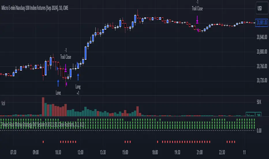
Power Hour Money StrategyDescription of the Pine Script Code: "Power Hour Money Strategy"
This Pine Script strategy, "Power Hour Money Strategy," is designed to trade based on the alignment of multiple time frames (month, week, day, and hour). The strategy aims to enter long or short positions depending on whether all selected time frames are in sync (all green for long positions, all red for short positions). Additionally, the script includes configurations for trading during specific sessions and automatically closing positions at the end of the trading day.
Core Features:
1. Time Frame Sync Check:
- The strategy evaluates whether the current price is higher than the opening price for the month, week, day, and hour to determine if each time frame is "green" (bullish) or "red" (bearish).
2. Session Control:
- The user can select between different trading sessions:
- "NY Session 9:30-11:30"
- "Extended NY Session 8-4"
- "All Sessions"
- Trades are only executed if the current time falls within the selected session.
3. Trailing Stop Mechanism:
- The strategy includes an optional trailing stop mechanism for both long and short positions.
- The trailing stop is configured with a percentage loss from the current price to protect gains.
4. End-of-Day Position Management:
- An option is provided to automatically close all positions at the end of the trading day (5:45 PM Eastern Time).
Detailed Code Breakdown:
1. Input Settings:
- **Session Selection**: Allows the user to choose the trading session.
- **End-of-Day Close**: Option to automatically close positions at the end of the day.
- **Trailing Stop Loss**: Enables or disables the trailing stop loss feature and sets the percentage for long and short positions.
2. Time Frame Calculations:
- The script uses `request.security` to get the opening prices for higher time frames (monthly, weekly, daily, and hourly).
- It compares the current close price to these opening prices to determine if each time frame is green or red.
3. Session Time Definitions:
- Defines the start and end times for the NY session (9:30-11:30 AM) and the extended session (8:00 AM - 4:00 PM).
4. Trade Execution:
- The strategy checks if all selected time frames are in sync and if the current time falls within the trading session.
- If all conditions are met, it enters a long or short position.
5. Trailing Stop Loss Implementation:
- Adjusts the stop price based on the trailing percentage and the current position's size.
- Automatically exits positions if the trailing stop condition is met.
6. End-of-Day Close Implementation:
- Uses a timestamp to check if the current time is 5:45 PM Eastern Time.
- Closes all positions if the end-of-day condition is met.
7. Plotting and Logging:
- Plots indicators to visualize the green/red status of each time frame.
- Logs information about the status of each time frame for debugging and analysis.
Example Usage:
Entering a Long Position: If the month, week, day, and hour are all green and the current time is within the selected session, a long position is entered.
Entering a Short Position: If the month, week, day, and hour are all red and the current time is within the selected session, a short position is entered.
Trailing Stop: Protects gains by exiting the position if the price moves against the set trailing stop percentage.
End-of-Day Close: Automatically closes all open positions at 5:45 PM Eastern Time if enabled.
This strategy is particularly useful for traders who want to ensure that multiple time frames are in alignment before entering a trade and who wish to manage positions effectively throughout the trading day with specific session controls and trailing stops.
ICT KillZones Hunt [TradingFinder] 4 Sessions + OB + FVG + Alert🔵 Introduction
🟣 ICT
The "ICT" style is a subset of "Price Action" technical analysis. The primary goal of the ICT trading strategy is to merge "Price Action" with the "Smart Money" concept to pinpoint optimal trade entry points.
However, this approach's strength extends beyond merely finding entry points. It also helps traders gain a deeper understanding of price behavior and adapt their trading strategies to the market structure.
The most important concepts of "ICT" :
Order Block
Fair Value Gap(FVG)
Liquidity
🟣 Session
Financial markets are divided into several time periods, each featuring distinct characteristics and levels of activity. These periods, known as sessions, are active at different times during the day.
The primary active sessions in financial markets include :
Asian Session
European Session
New York Session
Based on the UTC time zone, the schedule for these key sessions is :
Asian Session: 23:00 to 06:00
European Session: 07:00 to 16:30
New York Session: 13:00 to 22:00
Note
To avoid session overlap and minimize interference during kill zones, the session times have been modified as follows :
Asian Session: 23:00 to 06:00
European Session: 07:00 to 14:25
New York Session: 14:30 to 22:55
🟣 KillZone
Kill zones are periods within a session where trader activity spikes. During these times, trading volume surges, and price movements become more pronounced.
The major kill zones, according to the UTC time zone, are as follows :
Asian Kill Zone: 23:00 to 03:55
European Kill Zone: 07:00 to 09:55
New York Morning Kill Zone: 14:30 to 16:55
New York Evening Kill Zone: 19:30 to 20:55
🔵 How to Use
🟣 Order Block
Order blocks are a distinct category of "Supply and Demand" zones, formed when a series of orders are grouped together. These blocks are often created by banks or other significant market participants.
Banks typically execute large orders in blocks during their trading sessions. If they were to enter the market with small quantities, substantial price movements would occur before the orders were fully executed, reducing potential profit.
To mitigate this, they divide their orders into smaller, more manageable positions. Traders should seek "buy" opportunities in "demand order blocks" and "sell" opportunities in "supply order blocks."
🟣 Fair Value Gap (FVG)
To pinpoint the "Fair Value Gap" on the chart, meticulous candle-by-candle analysis is essential. Pay close attention to candles with significant bodies, examining each candle alongside the one preceding it.
The candles flanking this central candle should exhibit elongated shadows, with bodies that do not intersect the body of the central candle. The span between the shadows of the first and third candles is referred to as the FVG range.
Note :
The origin of all Order Blocks and FVGs starts from inside a kill zone and extends up to the end of the same session.
🟣 Kill Zone Hunt
Following this strategy, after the conclusion of the kill zone and the stabilization of its high and low lines, if the price touches either of these lines within the same session and encounters a robust rejection, it presents an opportunity to enter a trade.
🔵 Setting
🟣 Global Setting
Show All Order Block :
If it is turned off, only the last Order Block will be displayed.
Show All FVG :
If it is turned off, only the last FVG will be displayed.
Show More Info Session :
If it is turned on, more information about kill zones (Trade Volume, Time, Number of Candles) will be displayed.
🟣 Logic Parameter
Pivot Period of Order Blocks Detector :
Enter the desired pivot period to identify the Order Block.
Order Block Validity Period (Bar) :
You can specify the maximum time the Order Block remains valid based on the number of candles from the origin.
Mitigation Level Order Block :
Determining the basic level of a block order. When the price hits the basic level, the order block due to mitigation.
🟣 Order Blocks Display
Demand Order Block :
Show or not show and specify color.
Supply order Block :
Show or not show and specify color.
🟣 Order Block Refinement
Refine Demand OB :
Enable or disable the refinement feature. Mode selection.
Refine Supply OB :
Enable or disable the refinement feature. Mode selection.
🟣 FVG
FVG Validity Period (Bar) :
You can specify the maximum time the FVG remains valid based on the number of candles from the origin.
Mitigation Level FVG :
Determining the basic level of a FVG. When the price hits the basic level, the FVG due to mitigation.
Show Demand FVG :
Show or not show and specify color.
Show Supply FVG :
Show or not show and specify color.
FVG Filter :
Enable or disable filtering of FVGs. Select filter mode.
🟣 Session
Show More Info Session Color
Asia Session, London Sesseion, New York am Session & New York pm Session :
Show or not show session and kill zones. Change the display color.
🟣 Alert
Send Alert When Touched Session high & Low :
On / Off
Alert Demand OB Mitigation :
On / Off
Alert Supply OB Mitigation :
On / Off
Alert Demand FVG Mitigation :
On / Off
Alert Supply FVG Mitigation :
On / Off
Message Frequency :
This string parameter defines the announcement frequency. Choices include: "All" (activates the alert every time the function is called), "Once Per Bar" (activates the alert only on the first call within the bar), and "Once Per Bar Close" (the alert is activated only by a call at the last script execution of the real-time bar upon closing). The default setting is "Once per Bar".
Show Alert Time by Time Zone :
The date, hour, and minute you receive in alert messages can be based on any time zone you choose. For example, if you want New York time, you should enter "UTC-4". This input is set to the time zone "UTC" by default.
Display More Info :
Displays information about the price range of the order blocks (Zone Price) and the date, hour, and minute under "Display More Info". If you do not want this information to appear in the received message along with the alert, you should set it to "Off".

Volume-Enhanced Momentum Moving Average (VEMMA)Volume-Enhanced Momentum Moving Average (VEMMA)
Overview:
The Volume-Enhanced Momentum Moving Average (VEMMA) helps you spot market trends by combining momentum and volume as a moving average. This unique moving average adjusts itself based on the strength and activity of the market, giving you a clearer picture of what’s happening.
How It Works:
1. Key Settings (all of these are adjustable in the settings panel of the indicator):
◦ Base Length: Looks back over the last 50 days by default.
◦ Momentum Length: Uses the past 14 days to measure market strength.
◦ Volume Length: Uses the past 30 days to average trading volume.
◦ High/Low Thresholds: Considers RSI values above 70 as high momentum and below 30 as low momentum.
2. Momentum and Volume:
◦ Momentum: Calculated using the Relative Strength Index (RSI) to see if the market is gaining or losing strength.
◦ Volume: Average trading volume is calculated over the last 30 days to gauge trading activity.
3. VEMMA Calculation:
◦ For each of the past 50 days:
▪ Check Momentum: If RSI > 70, it’s high momentum; if RSI < 30, it’s low.
▪ Weight by Volume: High momentum days with high volume get more weight; low momentum days get less.
▪ Combine: Multiply the closing price by this weight and sum it up.
◦ Average: Divide the total by 50 to get the VEMMA value.
4. Visuals:
◦ Lines: Two lines, VEMMA1 (blue) and VEMMA2 (orange), show the adjusted moving averages.
◦ Colours: Background colors help you quickly spot high (green) and low (red) momentum periods.
How to Use:
• Spot Trends: Rising VEMMA lines suggest an uptrend; falling lines suggest a downtrend.
• Confirm Signals: When both VEMMA1 and VEMMA2 move together, it indicates a strong trend.
• Identify Reversals: Watch for background color changes from green to red or vice versa to catch potential trend reversals.
If the market has been strong and active, the VEMMA line will rise more sharply. If the market is weak and quiet, the line will be smoother.
Benefits:
• Integrated View: Combines market strength and trading activity for a fuller picture.
• Responsive: Adapts to significant market changes, highlighting key movements.
• Easy to Read: Clear visuals with color-coded backgrounds make interpretation simple.
Remember, just like any other indicator, this is not supposed to be used alone. Use it as part of your greater trading strategy. I do however believe it works exceptionally well for finding longer term trends early. The default VEMMA settings work very well as replacement for the EMA 200. Try it and see how it goes. Play around with the settings. Feedback appreciated.

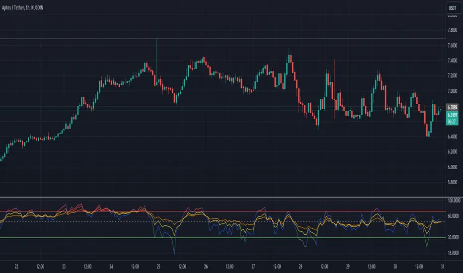
RSI Multiple TimeFrame, Version 1.0RSI Multiple TimeFrame, Version 1.0
Overview
The RSI Multiple TimeFrame script is designed to enhance trading decisions by providing a comprehensive view of the Relative Strength Index (RSI) across multiple timeframes. This tool helps traders identify overbought and oversold conditions more accurately by analyzing RSI values on different intervals simultaneously. This is particularly useful for traders who employ multi-timeframe analysis to confirm signals and make more informed trading decisions.
Unique Feature of the new script (described in detail below)
Multi-Timeframe RSI Analysis
Customizable Timeframes
Visual Signal Indicators (dots)
Overbought and Oversold Layers with gradual Background Fill
Enhanced Trend Confirmation
Originality and Usefulness
This script combines the RSI indicator across three distinct timeframes into a single view, providing traders with a multi-dimensional perspective of market momentum. It also provides associated signals to better time dips and peaks. Unlike standard RSI indicators that focus on a single timeframe, this script allows users to observe RSI trends across short, medium, and long-term intervals, thereby improving the accuracy of entry and exit signals. This is particularly valuable for traders looking to align their short-term strategies with longer-term market trends.
Signal Description
The script also includes a unique signal feature that plots green and red dots on the chart to highlight potential buy and sell opportunities:
Green Dots : These appear when all three RSI values are under specific thresholds (RSI of the shortest timeframe < 30, the medium timeframe < 40, and the longest timeframe < 50) and the RSI of the shortest timeframe is showing an upward trend (current value is greater than the previous value, and the value two periods ago is greater than the previous value). This indicates a potential buying opportunity as the market may be shifting from an oversold condition.
Red Dots : These appear when all three RSI values are above specific thresholds (RSI of the shortest timeframe > 70, the medium timeframe > 60, and the longest timeframe > 50) and the RSI of the shortest timeframe is showing a downward trend (current value is less than the previous value, and the value two periods ago is less than the previous value). This indicates a potential selling opportunity as the market may be shifting from an overbought condition.
These signals help traders identify high-probability turning points in the market by ensuring that momentum is aligned across multiple timeframes.
Detailed Description
Input Variables
RSI Period (`len`) : The number of periods to calculate the RSI. Default is 14.
RSI Source (`src`) : The price source for RSI calculation, defaulting to the average of the high and low prices (`hl2`).
Timeframes (`tf1`, `tf2`, `tf3`) : The different timeframes for which the RSI is calculated, defaulting to 5 minutes, 1 hour, and 8 hours respectively.
Functionality
RSI Calculations : The script calculates the RSI for each of the three specified timeframes using the `request.security` function. This allows the RSI to be plotted for multiple intervals, providing a layered view of market momentum.
```pine
rsi_tf1 = request.security(syminfo.tickerid, tf1, ta.rsi(src, len))
rsi_tf2 = request.security(syminfo.tickerid, tf2, ta.rsi(src, len))
rsi_tf3 = request.security(syminfo.tickerid, tf3, ta.rsi(src, len))
```
Plotting : The RSI values for the three timeframes are plotted with different colors and line widths for clear visual distinction. This makes it easy to compare RSI values across different intervals.
```pine
p1 = plot(rsi_tf1, title="RSI 5m", color=color.rgb(200, 200, 255), linewidth=2)
p2 = plot(rsi_tf2, title="RSI 1h", color=color.rgb(125, 125, 255), linewidth=2)
p3 = plot(rsi_tf3, title="RSI 8h", color=color.rgb(0, 0, 255), linewidth=2)
```
Overbought and Oversold Levels : Horizontal lines are plotted at standard RSI levels (20, 30, 40, 50, 60, 70, 80) to visually identify overbought and oversold conditions. The areas between these levels are filled with varying shades of blue for better visualization.
```pine
h80 = hline(80, title="RSI threshold 80", color=color.gray, linestyle=hline.style_dotted, linewidth=1)
h70 = hline(70, title="RSI threshold 70", color=color.gray, linestyle=hline.style_dotted, linewidth=1)
...
fill(h70, h80, color=color.rgb(33, 150, 243, 95), title="Background")
```
Signal Plotting : The script adds green and red dots to indicate potential buy and sell signals, respectively. A green dot is plotted when all RSI values are under specific thresholds and the RSI of the shortest timeframe is rising. Conversely, a red dot is plotted when all RSI values are above specific thresholds and the RSI of the shortest timeframe is falling.
```pine
plotshape(series=(rsi_tf1 < 30 and rsi_tf2 < 40 and rsi_tf3 < 50 and (rsi_tf1 > rsi_tf1 ) and (rsi_tf1 > rsi_tf1 )) ? 1 : na, location=location.bottom, color=color.green, style=shape.circle, size=size.tiny)
plotshape(series=(rsi_tf1 > 70 and rsi_tf2 > 60 and rsi_tf3 > 50 and (rsi_tf1 < rsi_tf1 ) and (rsi_tf1 < rsi_tf1 )) ? 1 : na, location=location.top, color=color.red, style=shape.circle, size=size.tiny)
```
How to Use
Configuring Inputs : Adjust the RSI period and source as needed. Modify the timeframes to suit your trading strategy.
Interpreting the Indicator : Use the plotted RSI values to gauge momentum across different timeframes. Look for overbought conditions (RSI above 70, 60 and 50) and oversold conditions (RSI below 30, 40 and 50) across multiple intervals to confirm trade signals.
Signal Confirmation : Pay attention to the green and red dots that provide signals to better time dips and peaks. dots are printed when the lower timeframe (5mn by default) shows sign of reversal.
These signals are more reliable when confirmed across all three timeframes.
This script provides a nuanced view of RSI, helping traders make more informed decisions by considering multiple timeframes simultaneously. By combining short, medium, and long-term RSI values, traders can better align their strategies with overarching market trends, thus improving the precision of their trading actions.

KillZones Hunt + Sessions [TradingFinder] Alert & Volume Ranges🟣 Introduction
🔵 Session
Financial markets are divided into various time segments, each with its own characteristics and activity levels. These segments are called sessions, and they are active at different times of the day.
The most important active sessions in financial markets are :
1. Asian Session
2. European Session
3. New York Session
The timing of these major sessions based on the UTC time zone is as follows :
1. Asian Session: 23:00 to 06:00
2. European Session: 07:00 to 16:30
3. New York Session: 13:00 to 22:00
Note
To avoid overlap between sessions and interference in kill zones, we have adjusted the session timings as follows :
• Asian Session: 23:00 to 06:00
• European Session: 07:00 to 14:25
• New York Session: 14:30 to 22:55
🔵 Kill Zones
Kill zones are parts of a session where trader activity is higher than usual. During these periods, trading volume increases and price fluctuations are more intense.
The timing of the major kill zones based on the UTC time zone is as follows :
• Asian Kill Zone: 23:00 to 03:55
• European Kill Zone: 07:00 to 09:55
• New York Morning Kill Zone: 14:30 to 16:55
• New York Evening Kill Zone: 19:30 to 20:55
This indicator focuses on tracking the kill zone and its range. For example, once a kill zone ends, the high and low formed during it remain unchanged.
If the price reaches the high or low of the kill zone while the session is still active, the corresponding line is not drawn any further. Based on this information, various strategies can be developed, and the most important ones are discussed below.
🟣 How to Use
There are three main ways to trade based on the kill zone :
• Kill Zone Hunt
• Breakout and Pullback to Kill Zone
• Trading in the Trend of the Kill Zone
🔵 Kill Zone Hunt
According to this strategy, once the kill zone ends and its high and low lines no longer change, if the price reaches one of these lines within the same session and is strongly rejected, a trade can be entered.
🔵 Breakout and Pullback to Kill Zone
According to this strategy, once the kill zone ends and its high and low lines no longer change, if the price breaks one of these lines strongly within the same session, a trade can be entered on the pullback to that level.
Trading in the Trend of the Kill Zone
We know that kill zones are areas where high-volume trading occurs and powerful trends form. Therefore, trades can be made in the direction of the trend. For example, when an upward trend dominates this area, you can enter a buy trade when the price reaches a demand order block.
🟣 Features
🔵 Alerts
You can set alerts to be notified when the price hits the high or low lines of the kill zone.
🔵 More Information
By enabling this feature, you can view information such as the time and trading volume within the kill zone. This allows you to compare the trading volume with the same period on the previous day or other kill zones.
🟣 Settings
Through the settings, you have access to the following options :
• Show or hide additional information
• Enable or disable alerts
• Show or hide sessions
• Show or hide kill zones
• Set preferred colors for displaying sessions
• Customize the time range of sessions
• Customize the time range of kill zones

KillZones & Sessions [TradingFinder] Volume | Asia, London & NY🔵 Introduction
🟣 Session
The forex market operates 24 hours a day, 5 days a week, with only Saturdays and Sundays being off; traders often focus on one of the forex trading sessions instead of trying to trade in all markets 24 hours a day.
Trading sessions are time intervals during which a specific financial market is active and trades are conducted. The Asia, London, and New York sessions are the most important trading sessions throughout the 24-hour period, during which a significant amount of money and liquidity enters the market.
🟣 Kill Zone
Traders in financial markets profit from the difference between the price at which they buy or sell and the current market price. Traders have different time horizons for trading.
Among these, some traders engage in daily or even hourly trading and must operate during times when the market has desirable trading volumes and significant price movements.
Kill zones are segments of a session with higher trading volumes and price fluctuations compared to the rest of the session.
🔵 How to Use
🟣 Session Time
The "Asia Session" consists of two sessions: "Sydney" and "Tokyo." The beginning of this session, according to the "UTC" time zone, is at 23:00 and ends at 06:00. Similarly, the beginning of the "Asia KillZone," according to the "UTC" time zone, is at 23:00, and it ends at 03:55.
The "London Session" consists of two sessions: "Frankfurt" and "London." The beginning of this session, according to the "UTC" time zone, is at 07:00, and it ends at 14:25. Similarly, the beginning of the "London KillZone," according to the "UTC" time zone, is at 07:00, and it ends at 09:55.
The beginning of the "New York am" session, according to the "UTC" time zone, is at 14:30, and it ends at 19:25. Similarly, the beginning of the "New York am KillZone," according to the "UTC" time zone, is at 14:30, and it ends at 16:55.
The beginning of the "New York pm" session, according to the "UTC" time zone, is at 19:30, and it ends at 22:55. Similarly, the beginning of the "New York pm KillZone," according to the "UTC" time zone, is at 19:30, and it ends at 20:55.
Important : To prevent session overlap, the working hours of each session have slightly changed.
🔵 Features
🟣 Simultaneous Session and Kill Zone
With this indicator, you can simultaneously view the kill zone and session. High and low lines are used to indicate sessions, while filled areas with color represent kill zones. If you do not want to see kill zones, you can turn off the display settings.
🟣 Candle, Time, and Volume
Using the "More Info" feature, you can see the number of candles, elapsed time, and traded volume within the colored filled area.
🔵 Settings
•Show More Info: To display "More Info," you need to turn on this feature and turn it off whenever you don't need it.
• You can also customize these settings for each session separately :
o Display or hide session.
o Choose session color.
o Set session time range.
o Display or hide kill zone.
o Set kill zone time range.
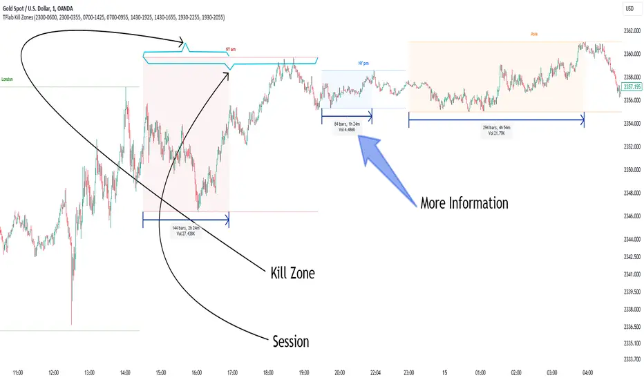
EMA Scalping StrategyEMA Slope Indicator Overview:
The indicator plots two exponential moving averages (EMAs) on the chart: a 9-period EMA and a 15-period EMA.
It visually represents the EMAs on the chart and highlights instances where the slope of each EMA exceeds a certain threshold (approximately 30 degrees).
Scalping Strategy:
Using the EMA Slope Indicator on a 5-minute timeframe for scalping can be effective, but it requires adjustments to account for the shorter time horizon.
Trend Identification: Look for instances where the 9-period EMA is above the 15-period EMA. This indicates an uptrend. Conversely, if the 9-period EMA is below the 15-period EMA, it suggests a downtrend.
Slope Analysis: Pay attention to the slope of each EMA. When the slope of both EMAs is steep (exceeds 30 degrees), it signals a strong trend. This can be a favorable condition for scalping as it suggests potential momentum.
Entry Points:
For Long (Buy) Positions: Consider entering a long position when both EMAs are sloping upwards strongly (exceeding 30 degrees) and the 9-period EMA is above the 15-period EMA. Look for entry points when price retraces to the EMAs or when there's a bullish candlestick pattern.
For Short (Sell) Positions: Look for opportunities to enter short positions when both EMAs are sloping downwards strongly (exceeding -30 degrees) and the 9-period EMA is below the 15-period EMA. Similar to long positions, consider entering on retracements or bearish candlestick patterns.
Exit Strategy: Use tight stop-loss orders to manage risk, and aim for small, quick profits. Since scalping involves short-term trading, consider exiting positions when the momentum starts to weaken or when the price reaches a predetermined profit target.
Risk Management:
Scalping involves high-frequency trading with smaller profit targets, so it's crucial to implement strict risk management practices. This includes setting stop-loss orders to limit potential losses and not risking more than a small percentage of your trading capital on each trade.
Backtesting and Optimization:
Before implementing the strategy in live trading, backtest it on historical data to assess its performance under various market conditions. You may also consider optimizing the strategy parameters (e.g., EMA lengths) to maximize its effectiveness.
Continuous Monitoring:
Keep a close eye on market conditions and adjust your strategy accordingly. Market dynamics can change rapidly, so adaptability is key to successful scalping.
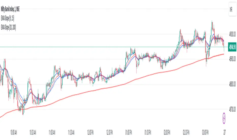
NASDAQ 100 Peak Hours StrategyNASDAQ 100 Peak Hours Trading Strategy
Description
Our NASDAQ 100 Peak Hours Trading Strategy leverages a carefully designed algorithm to trade within specific hours of high market activity, particularly focusing on the first two hours of the trading session from 09:30 AM to 11:30 AM GMT-5. This period is identified for its increased volatility and liquidity, offering numerous trading opportunities.
The strategy incorporates a blend of technical indicators to identify entry and exit points for both long and short positions. These indicators include:
Exponential Moving Averages (EMAs) : A short-term 9-period EMA and a longer-term 21-period EMA to determine the market trend and momentum.
Relative Strength Index (RSI) : A 14-period RSI to gauge the market's momentum.
Average True Range (ATR) : A 14-period ATR to assess market volatility and to set dynamic stop losses and trailing stops.
Volume Weighted Average Price (VWAP) : To identify the market's average price weighted by volume, serving as a benchmark for the trading day.
Our strategy uniquely applies a volatility filter using the ATR, ensuring trades are only executed in conditions that favor our setup. Additionally, we consider the direction of the EMAs to confirm the market's trend before entering trades.
Originality and Usefulness
This strategy stands out by combining these indicators within the NASDAQ 100's peak hours, exploiting the specific market conditions that prevail during these times. The inclusion of a volatility filter and dynamic stop-loss mechanisms based on the ATR provides a robust method for managing risk.
By focusing on the early trading hours, the strategy aims to capture the initial market movements driven by overnight news and the opening rush, often characterized by higher volatility. This approach is particularly useful for traders looking to maximize gains from short-term fluctuations while limiting exposure to longer-term market uncertainty.
Strategy Results
To ensure the strategy's effectiveness and reliability, it has undergone rigorous backtesting over a significant dataset to produce a sample size of more than 100 trades. This testing phase helps in identifying the strategy's potential in various market conditions, its consistency, and its risk-to-reward ratio.
Our backtesting adheres to realistic trading conditions, accounting for slippage and commission to reflect actual trading scenarios accurately. The strategy is designed with a conservative approach to risk management, advising not to risk more than 5-10% of equity on a single trade. The default settings in the script align with these principles, ensuring that users can replicate our tested conditions.
Using the Strategy
The strategy is designed for simplicity and ease of use:
Trade Hours : Focuses on 09:30 AM to 11:30 AM GMT-5, during the NASDAQ 100's peak activity hours.
Entry Conditions : Trades are initiated based on the alignment of EMAs, RSI, VWAP, and the ATR's volatility filter within the designated time frame.
Exit Conditions : Includes dynamic trailing stops based on ATR, a predefined time exit strategy, and a trend reversal exit condition for risk management.
This script is a powerful tool for traders looking to leverage the NASDAQ 100's peak hours, providing a structured approach to navigating the early market hours with a robust set of criteria for making informed trading decisions.

Auto-magnifier / quantifytools- Overview
Auto-magnifier shows a lower timeframe view of candles and volume bars inside any main timeframe candle by zooming into it. Candles and volume bars as they develop are shown chronologically from left to right. By default, magnifier is triggered when less than 3 candles are visible on the chart.
By default, 20 lower timeframe candles are displayed by splitting main timeframe into 20 parts. The amount of candles displayed is a target rate, meaning the script will use a lower timeframe that has the closest match to 20 candles and therefore will vary a bit. Users can override automatic timeframe calculation and opt in to display any specific lower timeframe or adjust amount of candles shown (e.g. 20 -> 30 candles) per each main timeframe candle.
Example
Main timeframe set to 30 minute, candles displayed set to 20 -> Magnifying using 2 minute candles (30 minute/20 candles = 1.5 min, rounded to 2 min)
Main timeframe set to 30 minute, override set to 5 minutes -> Displaying 5 minute candles
Size of volume bars is calculated using relative volume (volume relative to volume SMA20), lowest bar representing relative volume values of under or equal to 1x the moving average and from there onwards progressively growing.
- Limitations and considerations
Amount of candles shown might flow over from the background on smaller screen sizes, in which case you would want to decrease the amount shown. Opposite is true for bigger screens, this value can be increased as more candles fit.
This indicator involves a lot of tricks with text elements to make it work automatically by zooming in. Size of wicks, bodies and volume bars are calculated by adding more text elements on big candles and less text elements on smaller candles. This means the displayed candles won't be a 100% match, but a rather a fair representation of the view, e.g. candle is green = lower timeframe candle is green, candle has a big wick = lower timeframe candle has a big wick (but not a 100% match).
Example
Magnified lower timeframe chart vs. Actual lower timeframe chart
Most mismatch will be found on the price levels where lower timeframe candles are shown, which is sacrificed for the sake of getting a better readability on the overall shape of lower timeframe price action. Users can alternatively optimize calculations for more accuracy, giving a better representation of the price levels where candles truly originated. This typically comes with the cost of worse readability however.
Example
Optimized for readability vs. Optimized for accuracy
- Visuals
All visual elements are fully customizable.
