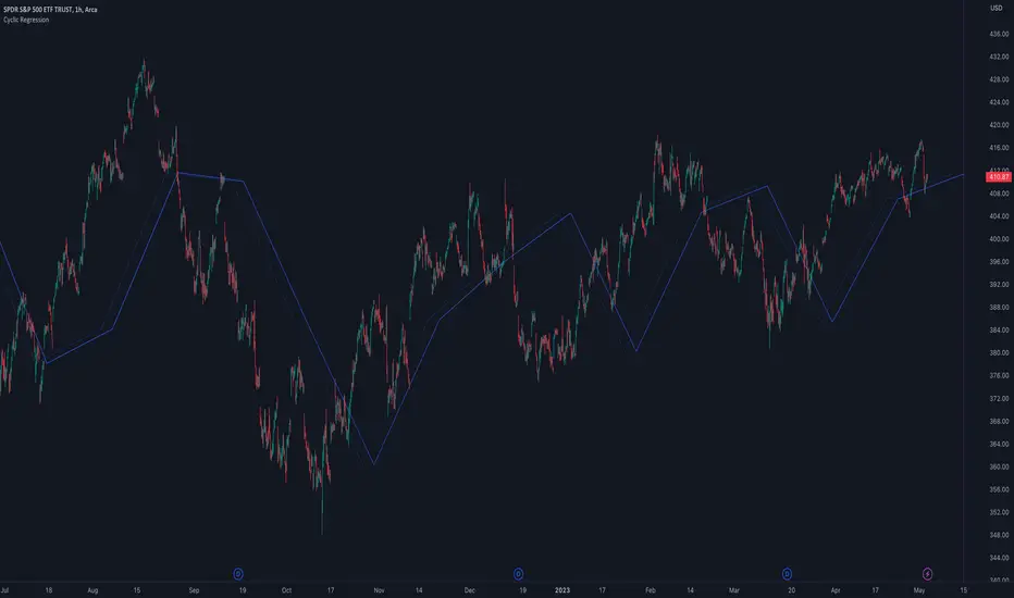
Bitcoin Puell Multiple (BPM)The Bitcoin Puell Multiple is a key indicator for evaluating buying and selling opportunities based on the profitability of Bitcoin miners.
The Idea
The Bitcoin Puell Multiple is a ratio that measures the daily profitability of Bitcoin miners in relation to the historical annual average of this profitability. It is calculated by dividing the amount of newly issued Bitcoins (in USD) each day by the 365-day moving average of that same amount. This indicator provides valuable information on Bitcoin's market cycles, helping investors to identify periods when Bitcoin is potentially undervalued or overvalued.
How to Use
To use the Bitcoin Puell Multiple, investors watch for extreme levels of the indicator. A high Puell Multiple suggests that miners are making exceptionally high profits compared to the previous year, which could indicate an overvaluation of Bitcoin and a selling opportunity (red zones). Conversely, a low Puell Multiple indicates that miners' earnings are low relative to history, suggesting an undervaluation of Bitcoin and a potential buying opportunity (green zones). The trigger thresholds for these zones can be configured in the tool's parameters.
What makes this tool different from the other "Puell Multiple" scripts available is that it is up to date in terms of its data sources, with a more precise calculation, and allows you to view the entire history.
Zone trigger limits and their visualization, as well as colors, are all configurable via the tool parameters.
Here, for example, is a configuration with more sensitive trigger levels and a different color:
Search in scripts for "Cycle"
BTC Halving [YinYangAlgorithms]This Indicator not only estimates what it thinks may be the PRICE for the Start, High and Low of the Halving, but likewise estimates WHEN the Start, High and Low of Halving may be. It then creates Trend Lines based on these predictions so that you may get an evaluation towards if the Price is currently Overbought or Oversold. These Trend Lines may be very useful for seeing the Slope in which the Price may move if it is to reach the estimated Price by the estimated Date. By evaluating the Prices location based on these Trend Lines we may determine if the Price is currently Overbought or Oversold.
These Trend Lines likewise may help identify locations of Support and Resistance. If the Price is much higher than its current Trend Line it is Overbought. There is a chance it will Consolidate back to the Trend Line or it may even correct with a dump all the way back to it; the opposite is true if it is much lower than its current Trend Line.
Trend Lines and Estimates are not all that is featured within this Indicator however. There are also Price Zones which may help identify if the price is currently:
Very Overbought (Red)
Slightly Overbought (Orange)
Neutral (Yellow)
Slightly Oversold (Teal)
Very Oversold (Green)
These zones may help give you an idea of how the price is currently fairing and its potential for movement. Likewise, it may help define where Support and Resistance may be found.
The trend line estimates are done with an algorithm created to evaluate the difference between price and % change that has occurred between the Start, High and Low of all the halvings over how many days between each data type. This may allow us to make an educated estimate towards what Price and Date the Start, High and Low will occur at.
Our Zones are created by evaluating the current Market Cap and circulating supply vs Max Supply of BTC. This may help give us an evaluation of what Price may be considered to be Overbought and Oversold; and likewise may help with estimations of where there may be Support and Resistance based on these Zones.
Tutorial:
In the example above we’re displaying the Halving Start Trend Line, our Information Tables and our Estimated Halving Vertical Marker. This Trend Line may help to display not only the trajectory and slope the Price needs to take to reach the Estimated Halving Price by the Estimated Halving Date; but it may also help to show if the price is Overvalued or Undervalued based on its position above or below this Trend Line.
Based on the Trajectory of the Estimated High Upward Trend Line (Green Line) in the photo above and from the ‘High Date’ estimated in the Information tables; we may attempt to estimate the location the ATH of this Bull Market will create and the price slope it may follow in doing so. This Trajectory may be very useful for understanding the price action that may occur for it to reach the High estimated Price by the High estimated Date.
We currently allow for two different types of zones within our Settings, one called ‘Fast’ displayed in the example above; and the other called ‘Slow’ displayed in the example below.
Our Fast Zone aims to move the Zone Levels Faster in an attempt to move with volatility and parabolic movement. This may help to keep the Very Overbought (Red) and Very OverSold (Green) Levels more accurate by attempting to keep the price within them. By doing so, we may aim to keep all of the Slightly Overbought, Slightly Oversold and Neutral Levels more accurate as well.
The Levels within these zones are defined by the Bright (less transparent) Lines. Whereas the Darker (more transparent) lines represent the Basis Lines between two different levels. These Basis lines may likewise act as a Support and Resistance Location too, but generally hold less weight than the actual Levels themselves.
What you may see is that during the Bull Market, the price is within the very Overbought Zones and even touches again the Very Overbought Level a few times. Likewise, during the Bear Market, the price is within the very Oversold Zones and even slightly drops below the Very Oversold Level. This may be expected and likewise may help to give estimates at potential for growth and decay within the Price based on which condition the Market is within.
Slow Zones move a little slower than Fast Zones, however they may still be accurate. Likewise, it is up to you to decide which Zone works better for your specific Trading Style; however, by default, the Zone type is set to Fast.
If you refer to both the Fast and Slow examples above, you may notice in the Fast the Price is only slightly above the ‘Slightly Oversold’ (Teal) line. Also, In the Fast, the Price where the ‘Very Overbought’ Level is 100k. This is one of the many reasons we’ve opted for ‘Fast’ as the default, and it is because it allows more room for movement; and in our opinion, potentially accuracy as well.
If you refer to the Slow example, you’ll see that the price is currently facing the Neutral Level as a Resistance location. However, if you refer to the price residing at the Slows ‘Very Overbought’ Level, it is only 81.5k, compared to the 100k of Fast.
The BTC Halving is a major event that takes place roughly every 4 years. It historically has a major impact on the market, and some may even say it signifies the Start, or close to start of the Bull Market. Therefore, since historically there may be cycles that BTC and potentially crypto itself follows, we’ve developed this Indicator in hopes that it may solve one of the biggest questions traders face. What Date will the Start, High and Low of the Halving occur and also at what Price.
Hopefully this Tutorial has given you some guidance as to how this Indicator may be used to help identify some of these key levels; including the slope at which the price may have to move if it is to reach its projection Price by its projected Date.
Settings:
1. Show Prediction Trend Lines:
- Options:
All
Start + High
Start + Low
High + Low
Start
High
Low
None
- Description:
Prediction Trend Lines may be an important way to see the Slope the Price needs to take to reach the Predicted Price by the Predicted Date. This may be useful for identifying if the Price is currently Overbought or Oversold.
2. Zone Type:
- Options:
Fast
Slow
- Description:
Zone types change the way the Zones expand.
3. Show Zones:
- Options:
All
Zones
Basis
None
- Description:
Zones are a way of seeing Overbought and Oversold Price locations based on Market Cap and Circulating Supply vs Max Supply.
4. Vertical Markers:
- Options:
All
Line
Label
None
- Description:
Vertical Markers display where the Halving has occurred with a Vertical Line and Label.
5. Show Tables:
Tables may be useful for seeing the Price and Date for when the Start, High and Low of the Halving may occur.
6. Fill Zones:
Filling in Zones may help to identify which Zone the Price is currently in.
If you have any questions, comments, ideas or concerns please don't hesitate to contact us.
HAPPY TRADING!
3x MTF MACD v3.0MACD's on 3 different Time Frames
Indicator Information
- Each Time Frame shows start of Trend and end of trend of the MACD vs the Signal Cross
- They are labled 1,2,3 with respective up or down triangle for possible direction.
User Inputs
- configure the indicator by specifying various inputs. These inputs include colors for bullish
and bearish conditions, the time frame to use, whether to show a Simple Moving Average
(SMA) line, and other parameters.
- Users can choose time frames for analysis (like 30 minutes, 1 hour, etc.)
but they must be in mintues.
- The code also allows users to customize how the indicator looks on the chart by providing
options for position and color.
Main Calculations
- The script calculates the Simple Moving Average (SMA) based on the user-defined time
frame.
- It then determines the color of the plot (line) based on certain conditions, such as whether
the SMA is rising or falling. These conditions help users quickly identify market trends.
Label Creation
- The code creates labels that can be displayed on the chart.
These labels indicate whether there's a bullish or bearish signal.
Level Detection
- The script determines and labels key levels or points of interest in the chart based on
certain conditions.
- It can show labels like "①" and "▲" for bullish conditions and "▼" for bearish conditions.
Table Display
- There's an option to show a table on the chart that displays information about the MACD
indicator Chosen and the NUmber Bubble assocated with that time frame
- The table can include information like which time frame is being analyzed, whether the SMA
line is shown, and other relevant data.
Plotting on the Chart
- The script plots the Simple Moving Average (SMA) on the chart. The color of this line
changes based on the calculated trend conditions.
ATR (Average True Range)
- The script also plots the Average True Range (ATR) on the chart. ATR is used to measure
market volatility.
"In essence, this script is a highly customizable MACD and SMA indicator for traders. It assists traders in comprehending market trends, offering insights into different MACD cycles concerning various timeframes.
Users can configure it to match their trading strategies, and it presents information in a user-friendly manner with colors, labels, and tables.
This simplifies market analysis, allowing traders to make more informed decisions without the distraction of multiple indicators."
Time Cycles IndicatorThis script is used to analyze the seasonality of any asset (commodities, stocks, indices).
To use the script select a timeframe D or W and select the months you are interested in the script settings. You will see all the candles that are part of those months highlighted in the chart.
You can use this script to understand if assets have a cyclical behavior in certain months of the year.
DB ZEMAThe DB ZEMA indicator is a no repaint indicator that is designed to local trends and local tops/bottoms. Since the indicator does not repaint, decisions can be made upon bar/period OPEN.
That means, when the indicator turns red indicating a market top is finished, then a decision can be made to close at the OPEN of that period. Likewise, when the indicator turns green, a decision can be made to buy at OPEN or during the current bar.
Additionally, traders may use the ZEMA level to get insight on the strength of the asset. For example, when the ZEMA is below -50 that would indicate a major low or weakness is present. ZEMAs under a certain threshold can indicate very good investment long entry points. Alternatively, zooming the chart out to view a long range of periods can show a pattern of common low ZEMA levels can be used as a baseline for good entry points. The same holds true for existing a long or entering a short.
Using a combination of the ZEMA color and the ZEMA level it's can be easy to tell smart entry and exist points. Especially on the weekly or higher timeframes.
For traders wanting real time data, there is a setting to disable the no-repaint mode to display the current real time ZEMA value. Traders may also adjust the length. By default the length of 10 is provided which is excellent for Weekly. We recommend a length of less than 10 for even high timeframes. For example a length of 2 is excellent on 4 Month timeframe for looking at market cycles, etc.
Finally the indicator offers the ability to change the symbol. This can be helpful in crypto in comparing the chart asset again BTC or similar.
Enjoy!
Hani angle support and resistanceBy examining the intersections of the average price in the past, this indicator identifies points as support and resistance, according to which it determines a diagonal line to the last average price in the future.
As you can see in the picture, these points are more important than floors and ceilings, and they can be cited more
According to the 360-period cycles of the market, it has the best performance
In this indicator, there are two lines that show the average price in different periods.
Ingulf candles and the pattern of three return candles are used for the signal
In the scalp model, the pattern of three consecutive candles and one engulfing candle is used
In the model of circles, Engulfing candle is also used according to algo
By default, this stop loss calculation is twice the size of the signal candle, which you can change according to the type of transaction.
Enter the amount of your balance and change the amount of contract size according to the currency
For example, the contract size is Bitcoin (1) and the contract size is EURUSD (100,000) and XAUUSD (100) and enter the amount of risk in each transaction.
At the time of the signal, you will see the exact size required to enter the transaction (not including the commission, because each exchange has a different commission and a different spread).
For a better view of the market, you can pay special attention to the distance and angle of the two lines.
Support and resistance lines are continuously displayed for 500 candles to be considered in the future of the market
This indicator requires basic knowledge of candlestick and it is better for the trader to make the final decision according to the market situation. However, an alarm has also been set that sends the stop loss amount for use in the web hook.
The price at the moment of the signal is also alarmed for comparison so that the signal can be compared at the time of the alarm.
The size of the ATR band is used to measure the wave if the waves are large enough to send cleaner signals.
The green label: distance between the last intersection and the average price.
The yellow label: distance between two periods of the average price
White label: lot size to enter the market
pink label: ATR size
Fair Value Gap Oscillator (Expo)█ Overview
The Fair Value Gap Oscillator (Expo) is an indicator based on the concept of Fair Value Gaps. It is a momentum indicator that helps traders identify mispricings in the market over time. The indicator also incorporates volume and volatility to increase its accuracy further. The indicator can be used in both trending and range-bound markets.
FVG occurs when there is an insufficient amount of buyers and sellers in the market for a particular asset. This can cause a sudden and large gap in the asset price, creating an imbalance in the price. This gap can be large enough to prevent traders from entering the market to take advantage of the price discrepancy. This, in turn, leads to a lack of liquidity and further price volatility.
█ How is the Fair Value Gap Oscialltor calculated?
The Fair Value Gap Oscillator is calculated by using historical Fair Value Gapa, volume, and volatility to determine if the market is trading at a discount or premium relative to its historical fair value. It is based on the idea that prices move in fair value cycles and that by looking at the oscillations of FVG data over time, traders can get a deeper insight into how imbalances impact the price over time.
█ Oscillator Trading
Oscillators are technical indicators that are used to measure momentum within a given market. These indicators measure the speed and magnitude of price movements. Traders use oscillators to identify potential entry and exit points in the market. They may look for overbought and oversold conditions, or they may look for divergence between the price of an asset and its oscillator. When these signals are identified, traders can then enter or exit positions accordingly.
█ How to use
It is a momentum indicator that helps traders identify mispricings in the market over time. In addition, the FVG Oscialltor can be used to identify overbought and oversold conditions in the market, as well as trends and leading trend changes.
Trending Indicator
The Fair Value Gap Oscillator can also be used to identify trends in the market. By tracking the FVG over time, investors can identify whether the market is trending up or down.
Leading Indicator
This indicator can be used to identify leading changes in the market’s momentum and price action. It will indicate beforehand when the momentum decreases and a potential trend change is about to come.
Divergences
Leading Indicators are great for identifying divergences. This Fair Value Gap Oscillator is a powerful yet simple tool to spot divergences in the market.
It is important to remember that the Fair Value Gap Oscillator is just one tool in your investment toolbox. It should be used in conjunction with other smart money concept indicators to identify excellent trading opportunities.
█ Indicator Features
Trend FVG
A Trend FVG feature is added to help Trend Traders get a long-term overview of the FVG trend. This feature can be used for the leading FVG calculation to get a predictive FVG trend.
Leading FVG Calculation
The leading calculation makes the Fair Value Gap oscillator sensitive to fair value changes and becomes more leading.
Trend Line
The Trend line feature is a combination of the leading and the long-term trend that can be used as trend confirmation.
-----------------
Disclaimer
The information contained in my Scripts/Indicators/Ideas/Algos/Systems does not constitute financial advice or a solicitation to buy or sell any securities of any type. I will not accept liability for any loss or damage, including without limitation any loss of profit, which may arise directly or indirectly from the use of or reliance on such information.
All investments involve risk, and the past performance of a security, industry, sector, market, financial product, trading strategy, backtest, or individual's trading does not guarantee future results or returns. Investors are fully responsible for any investment decisions they make. Such decisions should be based solely on an evaluation of their financial circumstances, investment objectives, risk tolerance, and liquidity needs.
My Scripts/Indicators/Ideas/Algos/Systems are only for educational purposes!
OECD CLI Diffusion IndexWhat does the indicator measure?
This is a macro indicator. It uses OECD's composite leading indicator - see details about the CLI below.
What it does it calculate YoY changes for CLI of 38 countries that are members or are associated with the OECD. Then it measures a percent of countries which CLI is rising.
How this can be used?
The positive slope of the curve means that there probably will be an economic growth among those countries within next 6 - 9 months. The negative slope means there probably will be an economic contraction.
Forward-looking economic growth is correlated with positive S&P 500 YoY growth (equity markets are also forward looking). The chart above presents the CLI diffusion index with overlayed S&P500 YoY rate of change.
The CLI is also correlated with ISM PMI - see example below:
What is a CLI?
"The OECD system of Composite Leading Indicators (CLIs) is designed to provide early signals of turning points in business cycles - fluctuation in the output gap, i.e. fluctuation of the economic activity around its long term potential level. This approach, focusing on turning points (peaks and troughs), results in CLIs that provide qualitative rather than quantitative information on short-term economic movements."
Mechanical Switch DetectorThis script reads volume as a voltage and picks up the mechanical signal of a switch. Instead of looking at the light globe to see when it turns on, this picks up the surge/pattern created when flicking on the switch. This picks up chart movements/cycles directly from the switches used in the ticker machine.. Faster than light.
Adjust "len" in the settings to select the sensitivity of the current used to calculate the threshold. 20 is default but try lengths of 200 or even 6 for smaller surges of current. This script assumes the ticker data is an analogue signal and picks up mechanical responses that are embedded within this signal. Nothing is random.
Time TradesThese indicators are part of the Time Trades service.
This script includes 2 timing indicators:
* Cheat Code displays green and purple timing periods
* Gann Waves displays yellow and blue vertical bars
Both indicators are based on natural cycles, and are visible into the future.
Visibility of both indicators is controlled via the Settings menu.
Cheat Code:
* Displays green periods and purple periods.
* Prices seem to trend more within a green period, both up and down.
* Often there’s major pivots around the middle of a green period, and about 3/4 through.
* Prices seem to chop more within a purple period with lots of volatility and reversals.
* Thin light grey lines appear at regular intervals that tend to align with local pivots.
* Thick grey lines appear around the middle of the green period that tens to align with major pivots
* You can use this information to vary your trading strategy to better match the expected price behavior.
Gann Waves
* Displays yellow and purple vertical bands that tend to align with local pivots.
* You can match this up with the symbol you’re analyzing to see what patterns tend to happen during similar periods.
* Sometimes stocks will make local highs for 3-4 yellow periods in a row, and then make a lower high. This would indicate a potential change in trend.
Stochastic DotsThese Stochastic Dots can help show potential turning points and cycles in the market.
- The smaller dots are based off of a faster moving stochastic
- The bigger dots are based off of a longer moving stochastic
- Dots below the candle/bar are bullish
- Dots above the candle/bar are bearish
This indicator is not meant to be traded by itself. Use other forms of confluency and confirmation with it.
If you're interested in more customized indicators to suit your needs, feel free to message me.
Cycle IndicatorA cycle indicator using a combination of hull and simple moving average, makes divergence very easy to see, colors are paired up when on either side of a trend when in a down trend uses red, with green for a pull back and when in up trend uses lime with maroon for the pull back, time entry when pull backs are back over zero line
oscillator fast cryptosmart (Bands on Scale)The oscillator fast cryptosmart is a high-sensitivity momentum indicator designed to generate signals more rapidly than many traditional oscillators, such as the MACD. It is engineered to detect potential price breakouts by analyzing short-term market cycles.
At its core, the indicator uses a Detrended Price Oscillator (DPO) to remove the longer-term trend from price action, allowing it to focus purely on the underlying momentum cycles. It then calculates dynamic volatility bands around this oscillator line.
Signals are generated when momentum breaks out from a normal range, providing traders with an early warning of a potential acceleration in price.
How to Interpret the Signals:
Buy Signal (Green Vertical Line): A buy signal is generated when the oscillator's main line (yellow) crosses above its upper statistical band. This indicates a sharp surge in positive momentum, suggesting a potential upward move is beginning.
Sell Signal (Red Vertical Line): A sell signal is generated when the oscillator's main line crosses below its lower statistical band. This indicates a significant increase in negative momentum, suggesting a potential downward move is starting.
By focusing on momentum breakouts rather than lagging moving average crossovers, the oscillator fast cryptosmart aims to provide an edge in identifying opportunities in fast-moving markets.
Smart Money Time (SMT)SMT Divergence – 90m / 30m / 10m (Prev-Cycle, Real-Time, Trailing)
Purpose:
This indicator finds SMT (Smart Money Technique) divergences between two related markets (e.g., CME_MINI:NQ1! vs CME_MINI:ES1! ). It does this per 90m/30m/10m cycles and only compares the current cycle to the immediately previous cycle —never older. It supports three cycle granularities:
90-minute cycles (9 blocks from 02:30–16:00 NY time)
30-minute sub-cycles (27 blocks)
10-minute sub-cycles (81 blocks; exactly 3 per 30-minute cycle)
For each cycle, the script tracks each symbol’s extreme (highest high for potential bearish SMT, lowest low for potential bullish SMT). When the leader sets a new extreme vs its own previous cycle while the lagger fails to do so vs its previous cycle, an SMT divergence is formed and plotted on the chart in real time. Lines trail as price makes new extremes within the same cycle.
What you’ll see on the chart:
A line from the previous cycle’s extreme to the current cycle’s extreme on the symbol pane where the indicator is applied (Primary A).
An optional text label at the current extreme (e.g., “90m SMT”, “30m SMT”, “10m SMT”).
Lines update (“trail”) as the current cycle goes on. When a new cycle begins, tracking resets for that cycle.
Default styling (editable):
90m SMT: solid, width 1, black
30m SMT: solid, width 1, black
10m SMT: dotted, width 1, black
You can toggle the text on/off and change width, style, and colors separately for 90m, 30m, and 10m.
Signals (definitions)
Bearish SMT: One market makes a Higher High vs its own previous cycle, while the other fails to make a Higher High vs its previous cycle.
Bullish SMT: One market makes a Lower Low vs its own previous cycle, while the other fails to make a Lower Low vs its previous cycle.
The line is drawn on Primary A by default.
Settings (explained)
Symbols
Primary Symbol A – the chart’s “leader/lagger” pane the script draws on.
Comparison Symbol B – the second market used for SMT checks.
Detection toggles
Detect SMT: 90m / 30m / 10m – turn on/off detection for each timeframe.
Note: The script always compares current cycle ↔ previous cycle only.
Validate candle direction
When enabled, the bar that makes the new extreme must also close in the confirming direction on that same market:
Bearish SMT: the bar that made the new Higher High must be a down close (close < open).
Bullish SMT: the bar that made the new Lower Low must be an up close (close > open).
This filter removes many “wick-only” probes and reduces false positives.
Turn off if you prefer to register SMTs on any intrabar extreme, regardless of bar close.
Delete SMT when invalidated
After an SMT forms, if the lagger later breaks the previous extreme it initially failed to break, the divergence is considered invalid and the script deletes the line and its label. (An “SMT invalidated” alert can fire if alerts are enabled.)
Enable alerts
Fires on SMT formed (separate messages for 90m/30m/10m and bullish/bearish) and on SMT invalidated.
To use, click Create Alert on the indicator and choose “Any alert() function call”. Use “Once per bar” (or per bar close) to taste.
Appearance – per timeframe (90m / 30m / 10m)
Bullish/Bearish colors, Line width, Line style, Show text (toggle subtitle label).
Text Options
Text color, Text size, Text offset (vertical spacing from the extreme).
How to use
Add to chart and select two related markets, e.g., NQ (A) vs ES (B).
Choose which cycles to monitor (90m / 30m / 10m).
Optionally enable Validate candle direction to demand a confirming close on the bar that made the extreme.
Watch for plotted SMTs:
Bearish SMT (HH vs no HH) often signals potential weakness
Bullish SMT (LL vs no LL) often signals potential strength
Use SMTs as context/confluence—e.g., near session highs/lows, liquidity pools, PD arrays, or your own levels. Combine with structure, order flow, and risk rules.
Turn on alerts to be notified when SMTs form or are invalidated in real time.
Notes & behavior
New-York session timing: Cycles are fixed windows in America/New_York and automatically handle DST.
Real-time & trailing: Lines trail to the most recent extreme within the same cycle but there’s no look-ahead across cycles.
No repaint across cycles: Each signal is strictly current cycle vs previous cycle.
Cleanup: On invalidation the script deletes the label first, then the line, preventing orphan labels.
Tips
10m SMTs are more frequent/noisier; 90m are fewer but more meaningful. Many traders look for multi-frame agreement (e.g., a 30m SMT aligning with a fresh 10m SMT).
If you want fewer signals, keep Validate candle direction on; if you want maximum sensitivity, turn it off.
Disclaimer: Educational use only. Markets are risky; do your own research and manage risk responsibly.
Empirical Kaspa Power Law Full Model v3.1🔶 First we need to understand what Power Laws are.
Power laws are mathematical relationships where one quantity varies as a power of another. They are prevalent in both natural and social systems, describing phenomena such as earthquake magnitudes, word frequencies, and wealth distributions. In a power-law relationship, a change in one quantity results in a proportional change in another, typically following a consistent and predictable mathematical pattern.
🔶 Why Do Power Laws work for Bitcoin and Kaspa?
Power laws work for Bitcoin and Kaspa due to the underlying principles of network dynamics and growth patterns that these cryptocurrencies exhibit. Here's how:
1. Network Growth and User Adoption:
Both Bitcoin and Kaspa grow as more users join their networks. The value of these networks often increases in a manner consistent with Metcalfe’s Law, which states that the value of a network is proportional to the square of its number of users. This relationship is a form of a power law, where network effects lead to exponential growth as more users participate.
2. Mining and Hash Rate:
The mining difficulty and hash rate in cryptocurrencies like Bitcoin and Kaspa adjust based on network activity. As more miners join, the difficulty increases to maintain a stable rate of block production. This self-adjusting mechanism creates feedback loops that can be described by power laws, ensuring the stability and security of the network over time.
3. Price Behavior:
Astrophysicist Giovanni Santostasi discovered that Bitcoin’s price follows a power-law distribution over time. This means that despite short-term volatility, Bitcoin’s long-term price behavior is predictable and adheres to specific mathematical patterns. Santostasi's model provides a framework for understanding Bitcoin’s price movements and forecasting future trends. He also discovered that Kaspa might be following a power-law aswell but it might be to early to tell because Kaspa hasn't been around for too long(2years).
4. Resource Allocation and System Stability:
As the price of Bitcoin or Kaspa increases, more resources are allocated to mining, leading to more sophisticated mining operations. This iterative process of investment and technological advancement follows a power-law pattern, driving the growth and stability of the network.
In summary, the application of power laws to Bitcoin and Kaspa offers a structured framework for understanding their price movements, network growth, and overall stability. These principles provide valuable predictive tools for long-term forecasting, helping to explain the dynamic behavior of these cryptocurrencies.
🔶 What does it look like on a chart?
Here is the Kaspa power law plotted on the KaspaUSD chart. Notice that the y-axis is in logarithmic scale. Unfortunately, TradingView does not allow the x-axis to be in logarithmic scale, which would otherwise make the power law appear as a straight line.
🔶 All the features of the Empirical Kaspa Power Law Full Model
This indicator includes a variety of scripts and tools, meticulously designed and developed to navigate the Kaspa market effectively.
🔹 Power Law & Deviation bands
The decision to use the lower two bands, marking an area between -40% to -50% below the power law, is based on historical analysis. Historically, this range has proven to be a great buying opportunity. In the case of Bitcoin, the bottom typically lies around -60% from the power law. However, for Kaspa, the bottom appears to be less distant from the power law. This discrepancy can be attributed to the differing supply dynamics of the two. Bitcoin undergoes a halving event approximately every four years, significantly reducing the rate at which new coins are introduced into circulation. This cyclical halving can lead to larger price fluctuations and a greater deviation from the power law. In contrast, Kaspa employs a more gradual reduction in its emission rate, with a 5% decrease each month. This consistent and incremental reduction helps Kaspa's price follow the power law more closely, resulting in less pronounced deviations. Consequently, the bottom for Kaspa tends to be closer to the power law, typically around -40% to -50%, rather than the -60% observed with Bitcoin.
The top two deviation bands are fitted to a few bubble data points, which are honestly not very reliable compared to the bottom bands that are based on a larger number of data points. When examining Bitcoin, we see that the bottoms are quite predictable due to the availability of thousands of data points, making it easier to identify patterns and trends.
However, predicting the tops is significantly more challenging because we lack a substantial amount of data for the peaks. This limited data makes it difficult to draw reliable conclusions about the upper deviation bands. As a result, while the bottom bands offer a robust framework for analysis, the top bands should be approached with caution due to their lesser reliability.
🔹 Alternating Sine wave
In observing the price behavior of Kaspa, an intriguing pattern emerges: it tends to follow a roughly four-month cycle. This cycle appears to alternate between smaller and larger waves. To capture this pattern, the sine wave in our indicator is designed to follow the power law, with both the top and bottom of the wave adjusting according to it.
Here's a simple explanation of how this works:
1. Four-Month Cycle: Empirically, Kaspa’s price seems to oscillate over approximately 120 days. This cycle includes periods of growth and decline, repeating every four months. Within these cycles, we observe alternating phases one smaller and one larger in amplitude.
2. Power Law Influence: The sine wave component of our indicator is not arbitrary; it follows a power law that predicts the general price trend of Kaspa. The power law essentially provides a baseline that reflects the longer-term price trajectory.
3. Diminishing Returns and Smoothing: To model diminishing returns, we adjust the amplitude of the sine wave over time, making it smaller as the cycle progresses. This helps to capture the natural tendency for price movements to become less volatile over longer periods. Additionally, the bottom of the sine wave adheres to the power law, ensuring it remains consistent with the overall trend.
🔹 Sine wave Cycle Start & End
Color transitions play a crucial role in visualizing different phases of the four-month cycle.
Based on empirical data, Kaspa experiences approximately 60 days of downward price action following each cycle peak, a period we refer to as the bear phase. This phase is followed by the bull phase, which also lasts around 60 days. To indicate the cycle peak, we have added a colored warning on the sine wave.
Cycle Start (Purple): The sine wave starts with a purple color, marking the beginning of a new cycle. This bull phase often represents a potential bottom or accumulation zone where prices are lower and stable, offering a strategic point for entering the market.
Cycle Top (Red): As the cycle progresses, the sine wave transitions through colors until it reaches red. This red phase indicates the top of the cycle, where the price is likely peaking. It's a critical area for investors to consider dollar-cost averaging (DCA) out of Kaspa, as it signifies a period of potential overvaluation and heightened risk.
These color transitions provide a visual guide to the market's cyclical nature, helping investors identify optimal entry and exit points. By following the sine wave's color changes, you can better time your investments, entering at the start of the cycle and considering exits as the cycle tops out.
🔹 Colored Deviation from the Power Law Bubbles
In trading, having a clear visual signal can significantly enhance decision-making, especially when dealing with complex models like power laws. This inspired the creation of the "deviation bubbles" in my indicator, which provides an intuitive, color-coded visual queue to help me, and other traders, better grasp market deviations and make timely trading decisions.
Here's a breakdown of how the deviation bubbles work:
1. Power Law Reference: The core of the indicator calculates a theoretical price level (the power law price) for Kaspa.
2. Deviation Calculation: For each day, the indicator computes the percentage deviation of the actual closing price from this power law price. This tells how much the market price diverges from the theoretically expected level.
3. Color-Coding Based on Deviation:
The deviation is categorized into various ranges (e.g., ≥ 100%, 90-100%, 80-90%, etc.).
Each range is assigned a distinct color, from red for extreme positive deviations to blue for extreme negative deviations.
This gradient helps in quickly identifying significant market deviations.
By integrating these bubbles into the chart, the indicator offers a simple yet powerful visual tool, aiding in recognizing critical market conditions without the need to delve into complex calculations manually. This approach not only enhances the ease of trading but also helps in overcoming the hesitation often faced when pulling the trigger on trades.
🔹 Projected Power Law Bands
Extends the current power law bands into the future using the same formula that defines the current power law.
Visual Representation: Dotted lines on the chart indicate the projected power law price and deviation bands.
Limitations: TradingView restricts how far these projections can extend, typically up to a reasonable future period.
These projected bands help anticipate future price movements, aiding in more informed trading decisions.
🔹 Projected Sine Wave
This projection continues to calculate the phase and amplitude, adjusting for diminishing returns and cycle transitions. It also estimates the future power law price, ensuring the projection reflects potential market dynamics.
Visual Representation: The projected sine wave is shown with dotted blue lines, providing a clear visual of the expected trend, aiding traders in their decision-making process.
Limitations: Again, TradingView restricts how far these projections can extend, typically up to a reasonable future period.
🔶 Why are all these different scripts made into one indicator?
As a trader and crypto analyst, I needed specific tools and customizations that no other indicator offered. Being a visual person, I rely heavily on visual triggers such as colors and patterns to make trading decisions. Initially, I developed this indicator for my personal use to enhance my market analysis with these visual cues. However, after sharing my insights, other traders expressed interest in using it. In response, I expanded the functionality and added various options to cater to a broader range of users.
This comprehensive indicator integrates multiple features into one tool, providing a powerful and flexible solution for analyzing market trends and making informed trading decisions. The use of colors and visual elements helps in quickly identifying key signals and market phases. The customizable options allow you to fine-tune the indicator to suit your specific needs, making it a versatile tool for both novice and experienced traders.
🔶 Usage & Settings:
This indicator is best used on the Daily chart for KASUSD - crypto because it uses a power law formula based on days.
🔹 Using the Indicator for 4-Month Cycles:
For traders interested in playing the 4-month cycles, this indicator provides a straightforward strategy. When the bubbles turn purple or the sine wave shows the purple start color, it signals a good time to dollar-cost average (DCA) into the market. Conversely, when the bubbles turn red or the cycle top is near, indicated by a red color, it’s time to DCA out of the Kaspa market. This visual approach helps traders make timely decisions based on color-coded signals, simplifying the trading process.
Historically, it was nearly impossible to accurately time all the 4-month cycle tops because they alternate each time. Without the combination of multiple scripts in this indicator, identifying these cyclical patterns and their respective peaks was extremely challenging. This integrated tool now provides a clear and reliable method for detecting these critical points, enhancing trading effectiveness.
🔹 Combining the visual queues for market extremes
The chart above illustrates the alignment of visual cues indicating market extremes. Notably, these visual cues—marked by red and purple boxes—historically pinpoint areas of extreme value or opportunities. When red aligns with red and purple aligns with purple, these zones have consistently indicated significant market extremes.
Understanding and recognizing these patterns provides a strategic advantage. By identifying these visual triggers, traders can plan and execute informed trades with greater confidence whenever similar scenarios unfold in the future.
Kaspa is perhaps one of the most cyclical and predictable cryptocurrencies in the market. Given its consistent behavior, traders might wonder why they would trade anything else. As long as there are no signs indicating a change in Kaspa's cyclical nature, there is no reason to make significant alterations to our predictions. This makes Kaspa an attractive option for traders seeking reliable and repeatable trading opportunities.
🔹 Settings & customization:
As a visually-oriented trader, it is essential to customize the appearance of indicators to effectively navigate the Kaspa market. The Indicator offers extensive customization options, allowing users to modify the colors of various elements to suit their preferences. For example, users can adjust the colors of the deviation bubbles, deviation bands, sine wave, and power law to enhance visual clarity and focus on specific data points. This level of personalization not only enhances the overall user experience but also ensures that the visual representation aligns with unique trading strategies, making it easier to interpret complex market data.
Additionally, users can change the power law inputs and other parameters as shown in the image. For instance, the Power Law Intercept and Power Law Slope can be manually adjusted, allowing traders to update these values. This flexibility is crucial as the future power law for Kaspa may evolve/change.
🔶 Limitations
Like any technical analysis tool, the Empirical Kaspa Power Law Full Model indicator has limitations. It's based on historical data, which may not always accurately predict future market movements.
🔶 Credits
I want to thank Dr. Giovanni Santostasi · Professor of physics and Mathematics.
He was one of the first who applied the concept of the power law to Bitcoin's price movements, which has been instrumental in providing insights into the long-term growth and potential future value of Bitcoin. Giovanni also offers coding classes on his Discord, which I attended. He personally taught me how to code specific things in Pine Editor and Python, sparking my interest in developing my own indicator.
Additionally, I would like to extend my gratitude to the following individuals for their invaluable contributions in terms of ideas, theories, formulas, testing, and guidance:
Forgowork, PlanC, Miko Genno, Chancellor, SavingFace, Kaspapero, JJ Venema.
Ehlers Band-Pass FilterHeyo,
This indicator is an original translation from Ehlers' book "Cycle Analytics for Traders Advanced".
First, I describe the indicator as usual and later you can find a very insightful quote of the book.
Key Features
Signal Line: Represents the output of the band-pass filter, highlighting the dominant cycle in the data.
Trigger Line: A leading indicator derived from the signal line, providing early signals for potential market reversals.
Dominant Cycle: Measures the dominant cycle period by counting the number of bars between zero crossings of the band-pass filter output.
Calculation:
The band-pass filter is implemented using a combination of high-pass and low-pass filters.
The filter's parameters, such as period and bandwidth, can be adjusted to tune the filter to specific market cycles.
The signal line is normalized using an Automatic Gain Control (AGC) to provide consistent amplitude regardless of price swings.
The trigger line is derived by applying a high-pass filter to the signal line, creating a leading
waveform.
Usage
The indicator is effective in identifying peaks and valleys in the market data.
It works best in cyclic market conditions and may produce false signals during trending periods.
The dominant cycle measurement helps traders understand the prevailing market cycle length, aiding in better decision-making.
Quoted from the Book
Band-Pass Filters
“A little of the data narrowly passed,” said Tom broadly.
Perhaps the least appreciated and most underutilized filter in technical analysis is the band-pass filter. The band-pass filter simultaneously diminishes the amplitude at low frequencies, qualifying it as a detrender, and diminishes the amplitude at high frequencies, qualifying it as a data smoother.
It passes only those frequency components from input to output in which the trader is interested. The filtering produced by a band-pass filter is superior because the rejection in the stop bands is related to its bandwidth. The degree of rejection of undesired frequency components is called selectivity. The band-stop filter is the dual of the band-pass filter. It rejects a band of frequency components as a notch at the output and passes all other frequency components virtually unattenuated. Since the bandwidth of the deep rejection in the notch is relatively narrow and since the spectrum of market cycles is relatively broad due to systemic noise, the band-stop filter has little application in trading.
Measuring the Cycle Period
The band-pass filter can be used as a relatively simple measurement of the dominant cycle.
A cycle is complete when the waveform crosses zero two times from the last zero crossing. Therefore, each successive zero crossing of the indicator marks a half cycle period. We can establish the dominant cycle period as twice the spacing between successive zero crossings.
When we measure the dominant cycle period this way, it is best to widen the pass band of the band-pass filter to avoid distorting the measurement simply due to the selectivity of the filter. Using an input bandwidth of 0.7 produces an octave-wide pass band. For example, if the center period of the filter is 20 and the relative bandwidth is 0.7, the bandwidth is 14. That means the pass band of the filter extends from 13-bar periods to 27-bar periods.
That is, roughly an octave exists because the longest period is twice the shortest period of the pass band. It is imperative that a high-pass filter is tuned one octave below the half-bandwidth edge of the band-pass filter to ensure a nominal zero mean of the filtered output. Without a zero mean, the zero crossings can have a substantial error.
Since the measurement of the dominant cycle can vary dramatically from zero crossing to zero
crossing, the code limits the change between measurements to be no more than 25 percent.
While measuring the changing dominant cycle period via zero crossings of the band-pass waveform is easy, it is not necessarily the most accurate method.
Best regards,
simwai
Good Luck with your trading! 🙌
Thiru TimeCyclesThiru TimeCycles Indicator: Overview and Features
Based on the provided Pine Script code (version 6), the "Thiru TimeCycles" indicator is a comprehensive, customizable tool designed for intraday traders, particularly those following Smart Money Concepts (SMC), ICT (Inner Circle Trader) methodologies, and time-based cycle analysis. It overlays session-based boxes, lines, and labels on charts to highlight key trading windows, ranges, and structural levels. The indicator is timezone-aware (default GMT-4, e.g., New York time) and focuses on killzones (high-volatility sessions), Zeussy-inspired 90-minute macro cycles, and 30-minute sub-cycles. It's optimized for timeframes below 4H, with automatic hiding on higher timeframes like 1D, 1W, 1M, or 1Y.
This indicator is ideal for forex, indices (e.g., Nasdaq futures like MNQ1!), stocks, and commodities, helping traders identify order flow, liquidity zones, and potential reversals within structured time cycles. It's built by Thiru Trades and includes educational elements like range tables and watermarks for a professional setup.
Core Purpose
Time Cycle Visualization: Breaks the trading day into repeatable cycles (e.g., 30-min, 90-min, and larger sessions) to anticipate market behavior, such as accumulation, manipulation, and distribution (AMD) phases.
Session Highlighting: Draws boxes and lines for major sessions (Asia, London, NY AM/PM, Lunch, Power Hour) to focus on high-probability "killzones."
Range and Pivot Analysis: Tracks highs/lows, midpoints, and ranges for each cycle/session, with optional alerts for breaks.
Customization Focus: Extensive inputs for colors, transparency, labels, and limits, making it adaptable for scalping, day trading, or swing setups.
Performance: Limits drawings to prevent chart clutter (e.g., max 500 boxes/lines/labels), with cutoff times to stop extensions (e.g., at 15:00).
Key Features
Here's a breakdown of the indicator's main components and functionalities, grouped by category:
Killzone Sessions (Standard Trading Windows):
Sessions Included: Asia (18:00-02:31), London (02:30-07:01), NY AM (07:00-11:31), Lunch (12:00-13:01), NY PM (11:30-16:01), Power Hour (15:00-16:01).
Visualization: Semi-transparent boxes (95% transparency default) with optional text labels (e.g., "London", "NY AM").
Pivots and Midpoints: Optional high/low pivot lines (solid style, extend until mitigated or cutoff), midpoints (dotted), and labels (e.g., "LO.H" for London High).
Alerts: Break alerts for pivots (e.g., "Broke London High").
Range Table: Optional table showing current and average ranges (over 5 sessions) for each killzone, positioned at top-right (customizable size/position).
Zeussy 90-Minute Macro Time Cycles:
Inspired By: Zeussy's time cycle theory (from X/Twitter), dividing sessions into 90-min phases starting at 02:30 NY time.
Cycles Included:
London: A (02:30-04:01, blue), M (04:00-05:31, red), D (05:30-07:01, green).
NY AM: A (07:00-08:31, blue), M (08:30-10:01, red), D (10:00-11:31, green).
NY PM/Lunch: A (11:30-13:01, blue), M (13:00-14:31, red), D (14:30-16:01, green).
Visualization: Boxes (90% transparency) with optional small labels ("London A", etc.) at the top of each box.
Extensions: High/low lines extend until broken or cutoff; optional equilibrium (EQ) levels.
Benefits: Helps identify AMD phases within larger sessions; focus on NY AM/PM for best results (Asia/London for global traders).
Zeussy 30-Minute Sub-Cycles:
Sub-Division: Further breaks 90-min cycles into 30-min segments (e.g., London A: A1 02:30-03:01, A2 03:00-03:31, A3 03:30-04:01).
All Sub-Cycles: 18 total (3 per macro cycle across London A/M/D, NY AM A/M/D, NY PM A/M/D).
Visualization: Optional boxes (90% transparency, hidden text by default) with small labels (e.g., "A1", "M1") at the bottom.
Customization: Separate show/hide toggle and label size (default "Small"); can divide further into 10-min if needed via presets.
Use Case: For finer granularity in scalping; shows order flow within macros (e.g., support at previous low after break).
Day Range Divider:
Vertical Separators: Dotted lines (custom color/width/style) at midnight (00:00) for each trading day (Mon-Fri only).
Day Labels: Monday-Friday labels (e.g., "Monday" with letter-spacing) positioned at the top of the chart (0.1% above high, updated dynamically).
Limits: Up to 5 days (customizable); hides on timeframes >=4H (1D, 1W, 1M, 1Y) to avoid clutter.
Offset: Labels above day-high by ticks (default 20); no weekend labels.
Fix Applied: Labels now consistently at top (using high * 1.001 for y-position); removed middle adjustments.
Day/Week/Month (DWM) Levels:
Opens, Highs/Lows, Separators: Lines for daily/weekly/monthly opens (dotted), previous highs/lows (solid), and vertical separators.
Unlimited Mode: Optional to show all history (otherwise limited by max_days).
Alerts: For high/low breaks (e.g., "Hit PDH").
Labels: Optional "D.O", "PWH" (previous week high), etc., with right-side extension.
Opening Prices and Vertical Timestamps:
Custom Opens: Up to 8 user-defined session opens (e.g., DC Open 18:00, 00:00, 09:30) with horizontal lines (dotted).
Vertical Lines: Up to 4 timestamps (e.g., 17:00, 08:00) with extend-both.
Unlimited: Optional to ignore drawing limits.
Range and Statistics Table:
Display: Top-right table (custom position/size) showing current range, average range (over 5 sessions), and min days stored for all enabled killzones/cycles.
Color-Coded: Rows highlight active sessions (e.g., Asia row in purple if active).
Toggle: Show/hide averages; updates on last bar.
Watermark and UI Enhancements:
Custom Watermark: Title ("ㄒ卄丨尺ㄩ"), subtitle ("PATIENCE | COURAGE | WISDOM"), symbol info (ticker + timeframe + date), positioned top-center/bottom-left.
Customization: Colors, sizes (tiny to huge), alignment (left/center/right), transparency.
Settings Groups: Organized into Settings, Killzones, Zeussy 90Min, Zeussy 30Min, Day Range Divider, Watermark, Pivots, Range, DWM, Opens, Vertical.
Performance and Limits:
Timeframe Limit: Hides drawings on >=240min (4H); Day Range hides on >=4H.
Drawing Limits: Max 1-5 days per type (boxes, lines, labels); auto-deletes old ones.
Cutoff: Optional stop at 15:00-15:01 for pivots/opens.
Alerts: Pivot breaks, high/low hits; freq once per bar.
Transparency: Separate for boxes (90-95%) and text (20-75%).
Continuous Partial Buying Signals v7.1🇬🇧 English Description: Continuous Partial Buying Signals v7.1
This indicator is built on a long-term accumulation philosophy , not a traditional buy-sell strategy. Its main purpose is to systematically increase your position in an asset you believe in by identifying significant price drops as buying opportunities. It is a tool designed for long-term investors who want to automate the "buy the dip" or "Dollar Cost Averaging (DCA)" mindset.
How It Works
The logic follows a simple but powerful cycle: Find a Peak -> Wait for a Drop -> Signal a Buy -> Wait for a New Peak.
1. Identifies a Significant Peak: Instead of reacting to minor price spikes, the indicator looks back over a user-defined period (e.g., the last 200 candles) to find the highest price. This stable peak (marked with an orange circle) becomes the reference point for the current cycle.
2. Waits for a Pullback: The indicator then calculates the percentage drop from this locked-in peak.
3. Generates Buy Signals: When the price drops by the percentages you define (e.g., -5% and -10%), it plots a "BUY" signal on the chart. It will only signal once per level within the same cycle.
4. Resets the Cycle: This is the key. If the price recovers and establishes a new significant peak higher than the previous one, the entire cycle resets. The new peak becomes the new reference, and the buy signals are re-armed, allowing the indicator to perpetually find new buying opportunities in a rising market.
How to Get the Most Out of This Indicator
* Timeframe: It is highly recommended to use this on higher timeframes (4H, Daily, Weekly) to align with its long-term accumulation philosophy.
* Peak Lookback Period:
* Higher values (200, 300): Create more stable and less frequent signals. Ideal for long-term, patient investors.
* Lower values (50, 100): More sensitive to recent price action, resulting in more frequent cycles.
* Drop Percentages: Adjust these based on the asset's volatility.
* Volatile assets (Crypto): Consider larger percentages like 10%, 20%.
* Less volatile assets (Stocks, Indices): Smaller percentages like 3%, 5%, 8% might be more appropriate.
This indicator is a tool for disciplined, emotion-free accumulation. It does not provide sell signals.
MERV: Market Entropy & Rhythm Visualizer [BullByte]The MERV (Market Entropy & Rhythm Visualizer) indicator analyzes market conditions by measuring entropy (randomness vs. trend), tradeability (volatility/momentum), and cyclical rhythm. It provides traders with an easy-to-read dashboard and oscillator to understand when markets are structured or choppy, and when trading conditions are optimal.
Purpose of the Indicator
MERV’s goal is to help traders identify different market regimes. It quantifies how structured or random recent price action is (entropy), how strong and volatile the movement is (tradeability), and whether a repeating cycle exists. By visualizing these together, MERV highlights trending vs. choppy environments and flags when conditions are favorable for entering trades. For example, a low entropy value means prices are following a clear trend line, whereas high entropy indicates a lot of noise or sideways action. The indicator’s combination of measures is original: it fuses statistical trend-fit (entropy), volatility trends (ATR and slope), and cycle analysis to give a comprehensive view of market behavior.
Why a Trader Should Use It
Traders often need to know when a market trend is reliable vs. when it is just noise. MERV helps in several ways: it shows when the market has a strong direction (low entropy, high tradeability) and when it’s ranging (high entropy). This can prevent entering trend-following strategies during choppy periods, or help catch breakouts early. The “Optimal Regime” marker (a star) highlights moments when entropy is very low and tradeability is very high, typically the best conditions for trend trades. By using MERV, a trader gains an empirical “go/no-go” signal based on price history, rather than guessing from price alone. It’s also adaptable: you can apply it to stocks, forex, crypto, etc., on any timeframe. For example, during a bullish phase of a stock, MERV will turn green (Trending Mode) and often show a star, signaling good follow-through. If the market later grinds sideways, MERV will shift to magenta (Choppy Mode), warning you that trend-following is now risky.
Why These Components Were Chosen
Market Entropy (via R²) : This measures how well recent prices fit a straight line. We compute a linear regression on the last len_entropy bars and calculate R². Entropy = 1 - R², so entropy is low when prices follow a trend (R² near 1) and high when price action is erratic (R² near 0). This single number captures trend strength vs noise.
Tradeability (ATR + Slope) : We combine two familiar measures: the Average True Range (ATR) (normalized by price) and the absolute slope of the regression line (scaled by ATR). Together they reflect how active and directional the market is. A high ATR or strong slope means big moves, making a trend more “tradeable.” We take a simple average of the normalized ATR and slope to get tradeability_raw. Then we convert it to a percentile rank over the lookback window so it’s stable between 0 and 1.
Percentile Ranks : To make entropy and tradeability values easy to interpret, we convert each to a 0–100 rank based on the past len_entropy periods. This turns raw metrics into a consistent scale. (For example, an entropy rank of 90 means current entropy is higher than 90% of recent values.) We then divide by 100 to plot them on a 0–1 scale.
Market Mode (Regime) : Based on those ranks, MERV classifies the market:
Trending (Green) : Low entropy rank (<40%) and high tradeability rank (>60%). This means the market is structurally trending with high activity.
Choppy (Magenta) : High entropy rank (>60%) and low tradeability rank (<40%). This is a mostly random, low-momentum market.
Neutral (Cyan) : All other cases. This covers mixed regimes not strongly trending or choppy.
The mode is shown as a colored bar at the bottom: green for trending, magenta for choppy, cyan for neutral.
Optimal Regime Signal : Separately, we mark an “optimal” condition when entropy_norm < 0.3 and tradeability > 0.7 (both normalized 0–1). When this is true, a ★ star appears on the bottom line. This star is colored white when truly optimal, gold when only tradeability is high (but entropy not quite low enough), and black when neither condition holds. This gives a quick visual cue for very favorable conditions.
What Makes MERV Stand Out
Holistic View : Unlike a single-oscillator, MERV combines trend, volatility, and cycle analysis in one tool. This multi-faceted approach is unique.
Visual Dashboard : The fixed on-chart dashboard (shown at your chosen corner) summarizes all metrics in bar/gauge form. Even a non-technical user can glance at it: more “█” blocks = a higher value, colors match the plots. This is more intuitive than raw numbers.
Adaptive Thresholds : Using percentile ranks means MERV auto-adjusts to each market’s character, rather than requiring fixed thresholds.
Cycle Insight : The rhythm plot adds information rarely found in indicators – it shows if there’s a repeating cycle (and its period in bars) and how strong it is. This can hint at natural bounce or reversal intervals.
Modern Look : The neon color scheme and glow effects make the lines easy to distinguish (blue/pink for entropy, green/orange for tradeability, etc.) and the filled area between them highlights when one dominates the other.
Recommended Timeframes
MERV can be applied to any timeframe, but it will be more reliable on higher timeframes. The default len_entropy = 50 and len_rhythm = 30 mean we use 30–50 bars of history, so on a daily chart that’s ~2–3 months of data; on a 1-hour chart it’s about 2–3 days. In practice:
Swing/Position traders might prefer Daily or 4H charts, where the calculations smooth out small noise. Entropy and cycles are more meaningful on longer trends.
Day trader s could use 15m or 1H charts if they adjust the inputs (e.g. shorter windows). This provides more sensitivity to intraday cycles.
Scalpers might find MERV too “slow” unless input lengths are set very low.
In summary, the indicator works anywhere, but the defaults are tuned for capturing medium-term trends. Users can adjust len_entropy and len_rhythm to match their chart’s volatility. The dashboard position can also be moved (top-left, bottom-right, etc.) so it doesn’t cover important chart areas.
How the Scoring/Logic Works (Step-by-Step)
Compute Entropy : A linear regression line is fit to the last len_entropy closes. We compute R² (goodness of fit). Entropy = 1 – R². So a strong straight-line trend gives low entropy; a flat/noisy set of points gives high entropy.
Compute Tradeability : We get ATR over len_entropy bars, normalize it by price (so it’s a fraction of price). We also calculate the regression slope (difference between the predicted close and last close). We scale |slope| by ATR to get a dimensionless measure. We average these (ATR% and slope%) to get tradeability_raw. This represents how big and directional price moves are.
Convert to Percentiles : Each new entropy and tradeability value is inserted into a rolling array of the last 50 values. We then compute the percentile rank of the current value in that array (0–100%) using a simple loop. This tells us where the current bar stands relative to history. We then divide by 100 to plot on .
Determine Modes and Signal : Based on these normalized metrics: if entropy < 0.4 and tradeability > 0.6 (40% and 60% thresholds), we set mode = Trending (1). If entropy > 0.6 and tradeability < 0.4, mode = Choppy (-1). Otherwise mode = Neutral (0). Separately, if entropy_norm < 0.3 and tradeability > 0.7, we set an optimal flag. These conditions trigger the colored mode bars and the star line.
Rhythm Detection : Every bar, if we have enough data, we take the last len_rhythm closes and compute the mean and standard deviation. Then for lags from 5 up to len_rhythm, we calculate a normalized autocorrelation coefficient. We track the lag that gives the maximum correlation (best match). This “best lag” divided by len_rhythm is plotted (a value between 0 and 1). Its color changes with the correlation strength. We also smooth the best correlation value over 5 bars to plot as “Cycle Strength” (also 0 to 1). This shows if there is a consistent cycle length in recent price action.
Heatmap (Optional) : The background color behind the oscillator panel can change with entropy. If “Neon Rainbow” style is on, low entropy is blue and high entropy is pink (via a custom color function), otherwise a classic green-to-red gradient can be used. This visually reinforces the entropy value.
Volume Regime (Dashboard Only) : We compute vol_norm = volume / sma(volume, len_entropy). If this is above 1.5, it’s considered high volume (neon orange); below 0.7 is low (blue); otherwise normal (green). The dashboard shows this as a bar gauge and percentage. This is for context only.
Oscillator Plot – How to Read It
The main panel (oscillator) has multiple colored lines on a 0–1 vertical scale, with horizontal markers at 0.2 (Low), 0.5 (Mid), and 0.8 (High). Here’s each element:
Entropy Line (Blue→Pink) : This line (and its glow) shows normalized entropy (0 = very low, 1 = very high). It is blue/green when entropy is low (strong trend) and pink/purple when entropy is high (choppy). A value near 0.0 (below 0.2 line) indicates a very well-defined trend. A value near 1.0 (above 0.8 line) means the market is very random. Watch for it dipping near 0: that suggests a strong trend has formed.
Tradeability Line (Green→Yellow) : This represents normalized tradeability. It is colored bright green when tradeability is low, transitioning to yellow as tradeability increases. Higher values (approaching 1) mean big moves and strong slopes. Typically in a market rally or crash, this line will rise. A crossing above ~0.7 often coincides with good trend strength.
Filled Area (Orange Shade) : The orange-ish fill between the entropy and tradeability lines highlights when one dominates the other. If the area is large, the two metrics diverge; if small, they are similar. This is mostly aesthetic but can catch the eye when the lines cross over or remain close.
Rhythm (Cycle) Line : This is plotted as (best_lag / len_rhythm). It indicates the relative period of the strongest cycle. For example, a value of 0.5 means the strongest cycle was about half the window length. The line’s color (green, orange, or pink) reflects how strong that cycle is (green = strong). If no clear cycle is found, this line may be flat or near zero.
Cycle Strength Line : Plotted on the same scale, this shows the autocorrelation strength (0–1). A high value (e.g. above 0.7, shown in green) means the cycle is very pronounced. Low values (pink) mean any cycle is weak and unreliable.
Mode Bars (Bottom) : Below the main oscillator, thick colored bars appear: a green bar means Trending Mode, magenta means Choppy Mode, and cyan means Neutral. These bars all have a fixed height (–0.1) and make it very easy to see the current regime.
Optimal Regime Line (Bottom) : Just below the mode bars is a thick horizontal line at –0.18. Its color indicates regime quality: White (★) means “Optimal Regime” (very low entropy and high tradeability). Gold (★) means not quite optimal (high tradeability but entropy not low enough). Black means neither condition. This star line quickly tells you when conditions are ideal (white star) or simply good (gold star).
Horizontal Guides : The dotted lines at 0.2 (Low), 0.5 (Mid), and 0.8 (High) serve as reference lines. For example, an entropy or tradeability reading above 0.8 is “High,” and below 0.2 is “Low,” as labeled on the chart. These help you gauge values at a glance.
Dashboard (Fixed Corner Panel)
MERV also includes a compact table (dashboard) that can be positioned in any corner. It summarizes key values each bar. Here is how to read its rows:
Entropy : Shows a bar of blocks (█ and ░). More █ blocks = higher entropy. It also gives a percentage (rounded). A full bar (10 blocks) with a high % means very chaotic market. The text is colored similarly (blue-green for low, pink for high).
Rhythm : Shows the best cycle period in bars (e.g. “15 bars”). If no calculation yet, it shows “n/a.” The text color matches the rhythm line.
Cycle Strength : Gives the cycle correlation as a percentage (smoothed, as shown on chart). Higher % (green) means a strong cycle.
Tradeability : Displays a 10-block gauge for tradeability. More blocks = more tradeable market. It also shows “gauge” text colored green→yellow accordingly.
Market Mode : Simply shows “Trending”, “Choppy”, or “Neutral” (cyan text) to match the mode bar color.
Volume Regime : Similar to tradeability, shows blocks for current volume vs. average. Above-average volume gives orange blocks, below-average gives blue blocks. A % value indicates current volume relative to average. This row helps see if volume is abnormally high or low.
Optimal Status (Large Row) : In bold, either “★ Optimal Regime” (white text) if the star condition is met, “★ High Tradeability” (gold text) if tradeability alone is high, or “— Not Optimal” (gray text) otherwise. This large row catches your eye when conditions are ripe.
In short, the dashboard turns the numeric state into an easy read: filled bars, colors, and text let you see current conditions without reading the plot. For instance, five blue blocks under Entropy and “25%” tells you entropy is low (good), and a row showing “Trending” in green confirms a trend state.
Real-Life Example
Example : Consider a daily chart of a trending stock (e.g. “AAPL, 1D”). During a strong uptrend, recent prices fit a clear upward line, so Entropy would be low (blue line near bottom, perhaps below the 0.2 line). Volatility and slope are high, so Tradeability is high (green-yellow line near top). In the dashboard, Entropy might show only 1–2 blocks (e.g. 10%) and Tradeability nearly full (e.g. 90%). The Market Mode bar turns green (Trending), and you might see a white ★ on the optimal line if conditions are very good. The Volume row might light orange if volume is above average during the rally. In contrast, imagine the same stock later in a tight range: Entropy will rise (pink line up, more blocks in dashboard), Tradeability falls (fewer blocks), and the Mode bar turns magenta (Choppy). No star appears in that case.
Consolidated Use Case : Suppose on XYZ stock the dashboard reads “Entropy: █░░░░░░░░ 20%”, “Tradeability: ██████████ 80%”, Mode = Trending (green), and “★ Optimal Regime.” This tells the trader that the market is in a strong, low-noise trend, and it might be a good time to follow the trend (with appropriate risk controls). If instead it reads “Entropy: ████████░░ 80%”, “Tradeability: ███▒▒▒▒▒▒ 30%”, Mode = Choppy (magenta), the trader knows the market is random and low-momentum—likely best to sit out until conditions improve.
Example: How It Looks in Action
Screenshot 1: Trending Market with High Tradeability (SOLUSD, 30m)
What it means:
The market is in a clear, strong trend with excellent conditions for trading. Both trend-following and active strategies are favored, supported by high tradeability and strong volume.
Screenshot 2: Optimal Regime, Strong Trend (ETHUSD, 1h)
What it means:
This is an ideal environment for trend trading. The market is highly organized, tradeability is excellent, and volume supports the move. This is when the indicator signals the highest probability for success.
Screenshot 3: Choppy Market with High Volume (BTC Perpetual, 5m)
What it means:
The market is highly random and choppy, despite a surge in volume. This is a high-risk, low-reward environment, avoid trend strategies, and be cautious even with mean-reversion or scalping.
Settings and Inputs
The script is fully open-source; here are key inputs the user can adjust:
Entropy Window (len_entropy) : Number of bars used for entropy and tradeability (default 50). Larger = smoother, more lag; smaller = more sensitivity.
Rhythm Window (len_rhythm ): Bars used for cycle detection (default 30). This limits the longest cycle we detect.
Dashboard Position : Choose any corner (Top Right default) so it doesn’t cover chart action.
Show Heatmap : Toggles the entropy background coloring on/off.
Heatmap Style : “Neon Rainbow” (colorful) or “Classic” (green→red).
Show Mode Bar : Turn the bottom mode bar on/off.
Show Dashboard : Turn the fixed table panel on/off.
Each setting has a tooltip explaining its effect. In the description we will mention typical settings (e.g. default window sizes) and that the user can move the dashboard corner as desired.
Oscillator Interpretation (Recap)
Lines : Blue/Pink = Entropy (low=trend, high=chop); Green/Yellow = Tradeability (low=quiet, high=volatile).
Fill : Orange tinted area between them (for visual emphasis).
Bars : Green=Trending, Magenta=Choppy, Cyan=Neutral (at bottom).
Star Line : White star = ideal conditions, Gold = good but not ideal.
Horizontal Guides : 0.2 and 0.8 lines mark low/high thresholds for each metric.
Using the chart, a coder or trader can see exactly what each output represents and make decisions accordingly.
Disclaimer
This indicator is provided as-is for educational and analytical purposes only. It does not guarantee any particular trading outcome. Past market patterns may not repeat in the future. Users should apply their own judgment and risk management; do not rely solely on this tool for trading decisions. Remember, TradingView scripts are tools for market analysis, not personalized financial advice. We encourage users to test and combine MERV with other analysis and to trade responsibly.
-BullByte
Cyclic Reversal Engine [AlgoPoint]Overview
Most indicators focus on price and momentum, but they often ignore a critical third dimension: time. Markets move in rhythmic cycles of expansion and contraction, but these cycles are not fixed; they speed up in trending markets and slow down in choppy conditions.
The Cyclic Reversal Engine is an advanced analytical tool designed to decode this rhythm. Instead of relying on static, lagging formulas, this indicator learns from past market behavior to anticipate when the current trend is statistically likely to reach its exhaustion point, providing high-probability reversal signals.
It achieves this by combining a sophisticated time analysis with a robust price-action confirmation.
How It Works: The Core Logic
The indicator operates on a multi-stage process to identify potential turning points in the market.
1. Market Regime Analysis (The Brain): Before analyzing any cycles, the indicator first diagnoses the current "personality" of the market. Using a combination of the ADX, Choppiness Index, and RSI, it classifies the market into one of three primary regimes:
- Trending: Strong, directional movement.
- Ranging: Sideways, non-directional chop.
- Reversal: An over-extended state (overbought/oversold) where a turn is imminent.
2. Adaptive Cycle Learning (The "Machine Learning" Aspect): This is the indicator's smartest feature. It constantly analyzes past cycles by measuring the bar-count between significant swing highs and swing lows. Crucially, it learns the average cycle duration for each specific market regime. For example, it learns that "in a strong trending market, a new swing low tends to occur every 35 bars," while "in a ranging market, this extends to 60 bars."
3. The Countdown & Timing Signal: The indicator identifies the last major swing high or low and starts a bar-by-bar countdown. Based on the current market regime, it selects the appropriate learned cycle length from its memory. When the bar count approaches this adaptive target, the indicator determines that a reversal is "due" from a timing perspective.
4. Price Confirmation (The Trigger): A signal is never generated based on timing alone. Once the timing condition is met (the cycle is "due"), the indicator waits for a final price-action confirmation. The default confirmation is the RSI entering an extreme overbought or oversold zone, signaling momentum exhaustion. The signal is only triggered when Time + Price Confirmation align.
How to Use This Indicator
- The Dashboard: The panel in the bottom-right corner is your command center.
- Market Regime: Shows the current market personality analyzed by the engine.
- Adaptive Cycle / Bar Count: This is the core of the indicator. It shows the target cycle length for the current regime (e.g., 50) and the current bar count since the last swing point (e.g., 45). The background turns orange when the bar count enters the "due zone," indicating that you should be on high alert for a reversal.
- BUY/SELL Signals: A label appears on the chart only when the two primary conditions are met:
The timing is right (Bar Count has reached the Adaptive Cycle target).
The price confirms exhaustion (RSI is in an extreme zone).
A BUY signal suggests a downtrend cycle is likely complete, and a SELL signal suggests an uptrend cycle is likely complete.
Key Settings
- Pivot Lookback: Controls the sensitivity of the swing point detection. Higher values will identify more significant, longer-term cycles.
- Market Regime Engine: The ADX, Choppiness, and RSI settings can be fine-tuned to adjust how the indicator classifies the market's personality.
- Require Price Confirmation: You can toggle the RSI confirmation on or off. It is highly recommended to keep it enabled for higher-quality signals.
90/30 Minute Cycle BoxesThis indicator automatically draws time-based cycle boxes to help visualize market structure and cyclical behavior.
Features:
90-Minute Primary Cycles: Highlights each 90-minute interval with a colored box, showing the high and low of that period.
30-Minute Sub-Cycles: Each 90-minute box is divided into 3 sub-boxes representing 30-minute phases.
Multi-Timeframe Compatible: Works on all timeframes, adapting dynamically to your chart.
Visual Clarity: Alternating box colors make it easy to track price action within and across cycles.
This tool is ideal for traders who use time cycles in their analysis, especially those applying ICT, Smart Money Concepts, or time-based market theories.
Bitcoin Destiny Line Model v1.1The Bitcoin Destiny Line Model
Table of Contents
1. Overview
2. Analytical and Technical Techniques Employed
3. Objectives of the Bitcoin Destiny Line Model
4. Key Technical Components and Functionalities
4.1. Bitcoin Destiny Line and Heatmap
4.2. Halving Cycles Markers
4.3. Dynamic Repricing Rails with Diminishing Volatility Adjustment
4.4. Seasonal Dynamics
4.5. Support and Resistance Zones
4.6. Market Action Indicators
4.7. Cycle Projections
4.8. Heatmap Only
5. Settings
6. Different Strategies to Utilize the Model
6.1. Value-Based Entry Strategy
6.2. Long-Term Position Strategy
6.3. Scaling Out Strategy
6.4. Portfolio Rebalancing Strategy
6.5. Bear Market Strategy
6.6. Short-Term Trading Strategy
7. Recommendations and Disclosures
1. Overview
The Bitcoin Destiny Line Model is a technical analysis toolset designed exclusively for Bitcoin. It integrates a comprehensive suite of analytical methodologies to provide deep insights into Bitcoin's market dynamics focusing on long-term investment strategies.
By analyzing historical data through various technical frameworks, the model helps investors gain insight into the current market structure, cycle dynamics, direction, and trend of Bitcoin, assisting investors and traders with data-driven decision-making.
2. Analytical and Technical Techniques Employed
The model integrates a range of analytical techniques:
Cycle Analysis - Centers on the Bitcoin halving event to anticipate phases within the Bitcoin cycle.
Logarithmic Regression Analysis - Calculates the logarithmic growth of Bitcoin over time.
Standard Deviation - Measures how significantly the price action differs from the long-term logarithmic trend.
Fibonacci Analysis - Identifies support and resistance levels.
Multi-Timeframe Momentum - Analyzes overbought or oversold conditions across multiple periods.
Trendlines - Draws trendlines from expected cycle lows to expected cycle highs extending logarithmic and deviation lines into the future as projection lines.
3. Objectives of the Bitcoin Destiny Line Model
The model is crafted to deliver an empirical framework for Bitcoin investing:
Bitcoin Market Structure - Offers insights into Bitcoin’s market structure.
Identify Value Opportunities and Risk Areas - Pinpoints potential value-entry opportunities and recognizes when the market is over-extended.
Leverage Market Cycles - Utilizes knowledge of Bitcoin’s seasonal dynamics and halving cycles to inform investment strategies.
Mitigate Downside Risk - Provides indicators for potential market corrections, aiding in risk management and avoidance of buying at peak prices.
4. Key Technical Components and Functionalities
4.1. Bitcoin Destiny Line and Heatmap
The cycle low to cycle high line with a risk-based color-coded heatmap serves as a central reference for Bitcoin’s price trajectory.
It emphasizes the long-term trend indicating areas of value in cool colors and areas of risk in warm colors.
4.2. Halving Cycles Markers
Bitcoin halving events are marked on the chart with vertical lines forming anchor points for cycle analysis.
4.3. Dynamic Repricing Rails with Diminishing Volatility Adjustment
Repricing rails based on the long-term logarithmic trend highlight the rails on which Bitcoin's price will reprice up or down.
Adjusts to the diminishing volatility of the asset over time as it matures.
4.4. Seasonal Dynamics
Integrates Bitcoin's inherent seasonal trends to provide additional context for market conditions aligning with broader market analysis.
Understanding Bitcoin’s seasons:
Spring Awakening - The initial recovery phase where the market begins to rebound from a bear market showing early signs of improvement. This is an ideal time for cautious optimism. Investors should consider gradually increasing their positions in Bitcoin, focusing on accumulation as confidence in market recovery grows.
Blossom Boom - A market bottom has been confirmed by now and market interest continues to pick up ahead of the Bitcoin halving. This typically presents a great opportunity for investors to position themselves advantageously ahead of expected price movements. It’s a good time to review and adjust portfolios to align with anticipated trends.
Midsummer Momentum - This phase follows the Bitcoin halving, characterized by a sideways to upward price trend often supported by heightened interest and media coverage. It represents potentially the last opportunity in the cycle for investors to purchase Bitcoin at lower price levels unlikely to be seen again. Investors should closely monitor the market for value buying opportunities to bolster their long-term investment strategies.
Rocket Rise - A phase where Bitcoin prices are likely to surge dramatically driven by a mix of Fear of Missing Out (FOMO) among new investors and widespread media hype. The strategy here is twofold: long-term holders should hold steady to reap maximum gains whereas more speculative investors might look to capitalize on the volatility by taking profits at optimal moments before a potential correction.
Winter Whispers - Following a bull run, the market begins to cool, marked by some investors taking profits and consequently increasing price fluctuations and volatility. During this time, investors should remain vigilant, tightening stop-loss orders to safeguard gains. This phase may be suitable for those looking to liquidate a portion of their long-term investments. However, for an investor to be selling the majority of their Bitcoin holdings is generally not advisable as it could preclude benefiting from potential future appreciations.
Deep Freeze - The market enters a bearish phase with significant price declines and market corrections. It's a period of consolidation and resetting of price levels. The end of this stage could typically be seen as a buying opportunity for the long-term investor. Accumulating Bitcoin during this phase can be advantageous as prices are lower and provide a foundation for significant growth in the next cycle.
4.5. Support and Resistance Zones
Calculates key levels that inform stop-loss placements and trading size decisions enhancing trading strategy around the Bitcoin Destiny Line.
4.6. Market Action Indicators
Suggests potential trading actions for different market phases aiding traders in identifying investment/trading opportunities.
Risk Indicator - Signals when prices are extremely over-extended helping to avoid entries during potential peak valuations.
4.7. Cycle Projections
Extends repricing levels into the future providing a visual forecast of expected price movements and enhancing strategic planning capabilities.
Cycle-High Price Projection Range - Provides a probabilistic range for upcoming cycle peaks based on historical trends and current market analysis.
4.8. Heatmap Only
It is also possible to plot the heatmap only as a background or as a bar in a second indicator.
4.9. Complete Visual View
A complete view of all key elements switched on the model.
5. Settings
Users can select to only show specific elements or all elements of the model.
They can set the sensitivity of some of the model elements and adjust certain view settings.
6. Different Strategies to Utilize the Model
The following strategies are enabled by the Bitcoin Destiny Line model:
6.1. Value-Based Entry Strategy
Investors can optimize their investment strategy by deploying investable cash either as a lump sum or on a dollar-cost averaging basis upon the display of a value indicator (Up-Triangles) which signals the highest probability for value entries.
6.2. Long-Term Position Strategy
As an alternative, investors may prefer to continue deploying investable funds while cooler colors (green or blue) are displayed on the value map, indicating favorable conditions for long-term positions.
6.3. Scaling Out Strategy
Investors may choose to scale out some of their investment upon the display of a risk indicator (circles) reducing exposure to potential downturns.
6.4. Portfolio Rebalancing Strategy
A sound strategy can also be to follow a portfolio rebalancing approach by deploying available investable cash upon the display of a value indicator. Rebalance the portfolio to maintain 25% in cash upon the display of a risk indicator. Adjust this ratio as subsequent risk indicators are triggered, deploying available cash upon future value signals.
6.5. Bear Market Strategy
In a bear market, traders may seek short positions upon the display of the Continued Downward Momentum indicator (Down Triangles) capitalizing on declining market trends.
6.6. Short-Term Trading Strategy
Traders can use hourly or 4-hourly data along with the daily Price Rails and Heatmap Bar for short-term positions. They may incorporate other preferred indicators such as RSI for entry/exit decisions.
7. Recommendations and Disclosures
Investors are recommended to take a prudent approach. It is not recommended for investors to scale out completely or significantly reduce the largest portion of their long-term Bitcoin positions in hopes of buying back at lower prices unless they have a compelling reason to do so. The future market conditions may not replicate past opportunities making this strategy uncertain. However, scaling out a smaller portion such as 25% can offer a high potential for an asymmetric risk-reward ratio. This approach is likely to provide a higher risk-adjusted return compared to traditional dollar-cost averaging or random lump sum adjustments.
The Bitcoin Destiny Line Model leverages 13.5 years of available price data across four complete Bitcoin market cycles.
While each additional cycle enriches the model's robustness and enhances the reliability of its forecasts, it is crucial for users to understand that historical trends are indicative of probable future directions and potential price ranges. Users should be cognizant that past performance is not a definitive predictor of future results and should not be the sole basis for investment decisions.