Patrones de entrada/salida V.1.0 -BETA-Este algoritmo intenta identificar patrones o fractales dentro de los movimientos de precios para dar señales de compra o venta de activos.
Search in scripts for "Fractal"

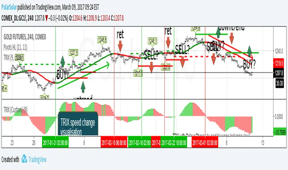
Triple Exponental Moving Average (overlay)TRIX Overlay + TRIX change Histogramm = simplest tactic to trade.
Just use last counter trend fractal to place delayed order
A counter trend fractal is a fractal down on TRIX uptrend or fractal up on TRIX downtrend.
Use TRIX speed change histogramm to seek divergence
Automatic Quadrant Lines📊 DETAILED EXPLANATION
Overview:
Automatic Quadrant Lines is a sophisticated pivot-based trading system that identifies key support and resistance levels, entry points, and price targets automatically. Based on fractal pivot analysis, this indicator creates a complete trading framework by mapping out potential long and short opportunities with precise entry and exit levels.
What Each Line Means:
Pivot Lines (Dark Red - Solid):
R1 (Resistance 1): The most recent pivot high - a key resistance level where price previously reversed downward
S1 (Support 1): The most recent pivot low - a key support level where price previously reversed upward. This line is thicker (weight 3) to emphasize its importance as the foundation for long setups
Entry Lines (Green/Red - Dashed or Solid):
L/E (Long Entry - Green Dashed): The trigger price for entering long positions. This is set at a strategic point above the pivot low, marking where bullish momentum is confirmed
S/E (Short Entry - Red Solid): The trigger price for entering short positions. This is set at a strategic point below the pivot high, marking where bearish momentum is confirmed
Long Target Lines (Green/Yellow/Cyan - Dashed):
Yellow Dashed Line (50%): First profit target for long positions - equal to one full range above the long entry
Cyan Dashed Line (75%): Second profit target for long positions - two full ranges above the long entry
Green Dashed Line (Long Target): Final profit target for long positions - three full ranges above the long entry, displayed with a dark green label showing the exact price
Short Target Lines (Red/Yellow/Cyan):
Yellow Line (50%): First profit target for short positions - equal to one full range below the short entry
Cyan Line (75%): Second profit target for short positions - two full ranges below the short entry
Red Line (Short Target): Final profit target for short positions - three full ranges below the short entry, displayed with a deep red label showing the exact price
Additional Lines:
Breakdown Target (Dark Green - Dashed): A support breakdown level located one range below S1, useful for managing risk if long positions fail
Technical Components:
Pivot Detection:
The indicator uses a configurable length (default 20) to identify swing highs and lows. A pivot high forms when the current high is the highest value over the specified length period on both sides. A pivot low forms when the current low is the lowest value over the specified period on both sides.
Entry Point Calculation:
Entry points are not placed at the pivot itself, but at strategic exit points of the pivot candle pattern. For long entries, the system identifies the high of the candle that preceded the pivot low. For short entries, it identifies the low of the candle that preceded the pivot high. This ensures entries occur on momentum confirmation rather than at turning points.
Target Calculation (Quadrant System):
The indicator calculates targets based on the range between the entry and the pivot (S1 for longs, R1 for shorts). It then projects this range upward (for longs) or downward (for shorts) in equal increments:
1x range = 50% target
2x range = 75% target
3x range = 100% target (Final Target)
Fractal Energy Filter:
The indicator incorporates a Fractal Energy (FE) calculation that measures market efficiency and trend strength. This helps filter entry signals, ensuring trades are taken only when market structure supports directional movement. The FE threshold can be adjusted in settings.
🎯 HOW TO USE (TRADER-FRIENDLY GUIDE)
📌 QUICK START GUIDE (IMPORTANT - Read This First!)
For optimal label visibility:
After adding this indicator to your chart for the first time, follow these ONE-TIME steps to ensure L/E and S/E labels are always visible:
Wait for the indicator to load and display L/E or S/E labels
Hover your mouse over any L/E or S/E label
Right-click on the label
Select "Bring to Front" or adjust "Visual Order" to bring it above price bars
Repeat for the other label type if needed
✅ You only need to do this ONCE - TradingView will remember this setting for all future labels!
If you ever want the labels to appear behind price bars again, simply right-click and select "Send to Back".
📈 For Long Trades:
Wait for Setup: The indicator automatically identifies a pivot low (S1 - thick dark red line) and calculates a long entry level (L/E - green dashed line with green label)
Entry Signal: When price crosses above the green L/E line, consider entering a long position. The system has confirmed bullish momentum
Profit Targets: Scale out of your position at the three target levels:
First target: Yellow dashed line (take 1/3 profit)
Second target: Cyan dashed line (take another 1/3 profit)
Final target: Green dashed line with "LONG TARGET" label (exit remaining position)
Stop Loss: Place your stop loss below the S1 level (thick dark red line). If price breaks below the dark green "Breakdown Target" line, consider exiting immediately
📉 For Short Trades:
Wait for Setup:
The indicator automatically identifies a pivot high (R1 - dark red line) and calculates a short entry level (S/E - red solid line with red label)
Entry Signal: When price crosses below the red S/E line, consider entering a short position. The system has confirmed bearish momentum
Profit Targets: Scale out of your position at the three target levels:
First target: Yellow line (take 1/3 profit)
Second target: Cyan line (take another 1/3 profit)
Final target: Red line with "SHORT TARGET" label (exit remaining position)
Stop Loss: Place your stop loss above the R1 level (dark red line)
💡 Key Trading Tips:
Color Coding: Remember GREEN = LONG, RED = SHORT throughout the entire system
Scaling Out: The three-target system allows you to lock in profits progressively while letting winners run
New Signals: When a new pivot forms, the indicator recalculates all levels. Old setups become invalid
Labels: The L/E and S/E labels mark the exact starting point of each entry line for easy identification
Price Display: Target labels show exact prices with proper comma formatting for easy reference
Timeframe: Works on any timeframe, but higher timeframes (4H, Daily) tend to produce more reliable signals
Customization: Adjust the Pivot Length (default 20) to make the system more responsive (lower number) or more stable (higher number)
⚠️ Risk Management:
Never risk more than 1-2% of your account per trade
The distance from entry to S1/R1 gives you a natural stop loss distance
Consider the full target distance when calculating position size
Not all setups will reach the final target - scaling out helps lock in profits
🔧 TROUBLESHOOTING
Q: My L/E or S/E labels are hidden behind candles
A: Right-click the label → "Bring to Front". This is a TradingView chart setting, not a script limitation. You only need to do this once.
Q: Can I hide the labels?
A: Yes! Uncheck "Show Labels" in the indicator settings.
Q: Can I adjust the label sizes?
A: Yes! Use the "Target Label Size" setting to adjust LONG/SHORT TARGET labels between Small, Normal, and Large.
Q: The labels moved when I clicked them
A: Labels are positioned automatically. If you accidentally moved them, simply refresh your chart.
Q: No signals are appearing
A: The indicator requires sufficient price history to detect pivots. Make sure you have at least 20+ bars on your chart. Try adjusting the Pivot Length setting.

DarkPool FlowDarkPool Flow is a professional-grade technical analysis tool designed to align retail traders with the dominant "smart money" flow. Unlike standard moving average crossovers that often generate false signals during consolidation, this script employs a multi-layered filtering engine to isolate high-probability trends.
The core philosophy of this indicator is that Trends are fractal. A sustainable move on a lower timeframe must be supported by momentum on a higher timeframe. By comparing a "Fast Signal Trend" against a "Slow Anchor Trend" (e.g., Daily vs. Weekly), the script identifies the market bias used by institutional algorithms.
This edition features a Smart Recovery Engine, ensuring that valid trends are not missed simply because momentum started slowly, and a Dynamic Cloud that visually represents the strength of the trend spread.
Key Features
1. Auto-Adaptive Timeframe Logic
The script eliminates the guesswork of Multi-Timeframe (MTF) selection. By enabling "Auto-Adapt," the indicator detects your current chart timeframe and automatically maps it to the mathematically correct institutional pairings:
Scalping (<15m): Uses 15-Minute Trend vs. 1-Hour Anchor.
Day Trading (15m - 1H): Uses 4-Hour Trend vs. Daily Anchor.
Swing Trading (4H - Daily): Uses Daily Trend vs. Weekly Anchor (The classic "Golden" setup).
Investing (Weekly): Uses 21-Week EMA vs. 50-Week SMA (Bull Market Support Band logic).
2. Smart Recovery Signal Engine
Standard crossover scripts often miss major moves if the specific breakout candle has low volume or weak ADX. This script utilizes a state-machine logic that "remembers" the trend direction. If a trend begins during low volatility (gray candles), the script waits. The moment volatility and momentum confirm the move, a Smart Recovery Signal is triggered, allowing you to enter an existing trend safely.
3. Chop Protection (Gray Candles)
Preservation of capital is the priority. The script analyzes the Average Directional Index (ADX) and Volatility (ATR).
Colored Candles (Green/Red): The market is trending with sufficient strength. Trading is permitted.
Gray Candles: The market is in a low-energy chop or consolidation (ADX < 20). Trading is discouraged.
4. Dynamic Trend Cloud
The space between the Fast and Slow trends is filled with a dynamic cloud.
Darker/Opaque Cloud: Indicates a widening spread, suggesting accelerating momentum.
Lighter/Transparent Cloud: Indicates a narrowing spread, suggesting the trend may be weakening or consolidating.
5. Pullback & Retest Signals (+)
While triangles mark the start of a trend, the Plus (+) signs mark low-risk opportunities to add to a position. These appear when price dips into the cloud, finds support at the "Fair Value" zone, and closes back in the direction of the trend with confirmed momentum.
User Guide & Strategy
Setup
Add the indicator to your chart.
For Beginners: Enable "Auto-Adaptive Timeframes" in the settings.
For Advanced Users: Disable Auto-Adapt and manually configure your Fast/Slow pairings (Default is Daily 50 EMA / Weekly 50 EMA).
Signal Mode: Choose "First Breakout Only" for a cleaner chart, or "All Signals" if you wish to see re-entry points during choppy starts.
Long Entry Criteria (Buy)
Trend: The Cloud must be Green (Fast Trend > Slow Trend).
Signal: A Green Triangle appears below the bar.
Confirmation: The signal candle must not be Gray.
Re-Entry: A small Green (+) sign appears, indicating a successful test of the cloud support.
Short Entry Criteria (Sell)
Trend: The Cloud must be Red (Fast Trend < Slow Trend).
Signal: A Red Triangle appears above the bar.
Confirmation: The signal candle must not be Gray.
Re-Entry: A small Red (+) sign appears, indicating a successful test of the cloud resistance.
Stop Loss & Risk Management
Stop Loss: A standard institutional stop loss is placed just beyond the Slow Trend Line (the outer edge of the cloud). If price closes beyond the Slow Trend, the macro thesis is invalid.
Take Profit: Target liquidity pools or use a trailing stop based on the Fast Trend line.
Settings Overview
Mode Selection: Toggle between Auto-Adaptive logic or Manual control.
Manual Configuration: Define the specific Timeframe, Length, and Type (EMA, SMA, WMA) for both Fast and Slow trends.
Signal Logic: Toggle "Show Pullback Signals" on/off. Switch between "First Breakout" or "All Signals."
Quality Filters: Toggle individual filters (ATR, RSI, ADX) to adjust sensitivity. Turning these off makes the script more responsive but increases false signals.
Visual Style: Customize colors for Bullish, Bearish, and Neutral (Gray) states. Adjust cloud transparency.
Disclaimer
Risk Warning: Trading financial markets involves a high degree of risk and is not suitable for all investors. You could lose some or all of your initial investment.
Educational Use Only: This script and the information provided herein are for educational and informational purposes only. They do not constitute financial advice, investment advice, trading advice, or any other recommendation.
No Guarantee: Past performance of any trading system or methodology is not necessarily indicative of future results. The "Institutional Trend" indicator is a tool to assist in technical analysis, not a crystal ball. The creators of this script assume no responsibility or liability for any trading losses or damages incurred as a result of using this tool. Always perform your own due diligence and consult with a qualified financial advisor before making investment decisions.

Elite S&D [By:CienF]Elite Supply & Demand
Description
Elite Supply & Demand is not just another zone indicator; it is a complete institutional trading system designed to identify high-probability imbalances in the market. Unlike standard indicators that flood the chart with weak zones, this script applies rigorous Price Action rules to filter, score, and validate only the most significant areas of interest.
The core philosophy of this tool is "Anormality". Institutional activity leaves a footprint in the form of explosive volatility relative to the recent context. This indicator detects these footprints, measures their intensity, and validates them against market structure.
Key Features
🔥 Dynamic Quality Scoring (The "Elite" Feature) The indicator doesn't just draw boxes; it rates them. It calculates a Volumetric Ratio comparing the explosive move against the historical average at the moment of creation.
Contextual Intelligence: It continues to track the initial move. If the momentum continues after a small pause, the score updates in real-time.
Visual Grades:
🔥 Fire: High Anormality (Institutional Imbalance).
⚡ Lightning: Moderate Anormality (Decent strength).
No Icon: Standard move.
🏗️ Advanced Structure Validation Includes a unique "Eventual Break" filter.
Latent Zones: You can choose to hide zones that haven't broken structure yet.
Auto-Validation: The zone remains invisible/transparent until price breaks a recent High/Low or Fractal Pivot. Once the break occurs, the zone "activates" on your chart.
🧠 Smart Mitigation Logic
No Zombie Zones: Once a zone is mitigated (touched), it is strictly processed. It can either turn gray (History Mode) or be removed instantly.
Priority Handling: Mitigated zones are never re-colored or re-validated, keeping your chart clean and accurate.
🚀 Performance Optimization
Date Lookback: Includes a "Days Back" filter to prevent the script from calculating thousands of historical candles, ensuring smooth performance even on lower timeframes (1m, 5m).
🔔 Integrated Alerts
Creation: Get notified immediately when a potential zone forms.
Validation: Get notified specifically when a latent zone breaks structure and becomes active.
How It Works ( The Logic)
Phase 1: The Base (Indecision): Identifies candles with small bodies (≤ 50% of range) representing equilibrium/accumulation.
Phase 2: The Explosion (Imbalance): Looks for a strong breakout candle (≥ 60% body) that moves away from the base.
Phase 3: The Follow-up: Verifies that the move continues. It allows for "Smart Pauses" (single indecision candles) within the trend but invalidates the zone if a reversal occurs immediately.
Phase 4: Structure Check: Verifies if the move broke the Recent Range (High/Low) or Fractal Pivots.
Settings & Configuration
1. Base & Exit Rules
Max % Body: Threshold to define an indecision candle (Default: 50%).
Explosive Min: Minimum strength required for the exit candle.
2. Structure Validation
Structure Type: Choose between Recent Range (more fluid) or Fractal Pivots (stricter).
Filter Eventual Break: Highly Recommended. If checked, zones appear only after they prove their strength by breaking structure.
3. Scoring (Quality)
High Quality Ratio: The multiplier required to earn the 🔥 icon (e.g., 2.0x larger than average).
Allow Pause: Allows the algorithm to capture larger moves even if there is a single small candle in the middle of the explosive leg.
4. Performance
Days Back: Limits how far back the indicator draws. Reduce this number on low timeframes to speed up loading.
Usage Recommendations
For Trend Trading: Look for "Follow-up" zones. If you see a 🔥 zone forming in the direction of the higher timeframe trend, it is a high-probability entry.
For Reversals: Use the "Filter Eventual Break" feature. Wait for the indicator to reveal a zone that has broken a major structure point.
Stop Loss Placement: The indicator draws the zone covering the entire "Base" (wicks included). A safe stop is typically just beyond the distal line (33% recommended) of the box.
🔔 How to Set Up Alerts
Since this indicator uses the dynamic alert() function to send detailed messages (Entry Price, Stop Zone, Type), you must configure it correctly:
Add the indicator to your chart and adjust the settings to your preference.
Click the "Create Alert" button (Clock Icon) on the right toolbar or press Alt + A.
Condition: Select "Elite S&D " from the dropdown menu.
Trigger (CRITICAL): You must select "Any alert() function call".
Note: Do not select "Crossing" or other standard conditions, or the alerts will not trigger.
Expiration: Select "Open-ended" (if you have a Premium plan) or set a future date.
Alert Actions: Choose where you want to receive the alert (Notify on App, Show Popup, Send Email, etc.).
Message: You can leave this default. The script automatically generates a detailed message with the Ticker, Timeframe, Zone Type, and Coordinates.
Click Create.
Disclaimer: This tool is designed to assist in technical analysis and does not constitute financial advice. Always use proper risk management.

PyraTime Harmonic 369Concept and Methodology PyraTime Harmonic 369 is a quantitative time-projection tool designed to apply Modular Arithmetic to market analysis. Unlike linear time indicators, this tool projects non-linear integer sequences derived from Digital Root Summation (Base-9 Reduction).
The core logic utilizes the mathematical progression of the 3-6-9 constants. By anchoring to a user-defined "Origin Pivot," the script projects three distinct harmonic triads to identify potential Temporal Confluence—moments where mathematical time cycles align with price action.
Technical Features This script focuses on the Standard Scalar (1x) projection of the Digital Root sequence:
The Root-3 Triad (Red): Projects intervals of 174, 285, 396. (Mathematical Sum: 1+7+4=12→3)
The Root-6 Triad (Green): Projects intervals of 417, 528, 639. (Mathematical Sum: 4+1+7=12→3, inverted)
The Root-9 Triad (Blue): Projects intervals of 741, 852, 963. (Mathematical Sum: 7+4+1=12→3... completion to 9)
How to Use
Set Anchor: Input the time of a significant High or Low in the settings.
Select Resolution: This tool is optimized for 1-minute (Micro-Harmonics) and 15-minute (Intraday Harmonics) charts.
Analyze Clusters: The vertical lines represent calculated harmonic intervals. Traders look for "Clusters" where a Root-3 and Root-9 cycle land on adjacent bars, indicating a high-probability pivot.
System Architecture & Version Comparison This script represents the foundational layer of the PyraTime ecosystem.
This Script (PyraTime Harmonic 369):
Scalar: Standard 1x Multiplier only.
Focus: Intraday & Micro-structure (1m, 15m).
Engine: Core Digital Root Integers.
PyraTime Harmonic Matrix (Advanced Edition):
Scalar Engine: Unlocks Quad-Fractal (4x), Tri-Fractal (3x), and Bi-Fractal (2x) multipliers for institutional cycle analysis.
Apex Logic: Auto-detection of the "963" Completion Sequence (Gold Highlight).
Event Horizon: Includes a live Predictive Dashboard that calculates the time-delta to the next harmonic event across all scalar groups.
Disclaimer This tool is for the educational analysis of Number Theory in financial markets. It projects time intervals and does not predict price direction. Past performance does not guarantee future results.

SR-ZnV2There are many support and resistance scripts out there. I was unable to find one that met all of my needs so I have expanded on the closest ones that I was able to discover. The ability to show persistent S/R levels by volume at various time frames automates much of the process for the user with unique and customizable features, the lastest dated of which are displayed by its time frame support/resistance strength and extend toward the right of the screen where they can be seen more clearly by price .
// Original script is thanks to tommyf1001, synapticex and additional modifications is thanks to Lij_MC. Credit to both of them for most of the logic behind this script. Since then I have made many changes to this script as noted below.
// Changed default S/R lines from plots to lines, and gave option to user to change between solid line, dashed line, or dotted line for both S/R lines.
// Added additional time frame and gave more TF options for TF1 other than current TF. Now you will have 4 time frames to plot S/R zones from.
// Gave user option to easily change line thickness for all S/R lines.
// Made it easier to change colors of S/R lines and zones by consolidating the options under settings (rather than under style).
// Added extensions to active SR Zones to extend all the way right.
// Added option to extend or not extend the previous S/R zones up to next S/R zone.
// Added optional time frame labels to active S/R zones, with left and right options as well as option to adjust how far to the right label is set.
// Fixed issue where the higher time frame S/R zone was not properly starting from the high/low of fractal. Now any higher time frame S/R will begin exactly at the High/Low points.
// Added to script a function that will prevent S/R zones from lower time frames displaying while on a higher time frame. This helps clean up the chart quite a bit.
// Created arrays for each time frame's lines and labels so that the number of S/R zones can be controlled for each time frame and limit memory consumption.
// New alert options added and customized alert messages.

Stochastic Enhanced [DCAUT]█ Stochastic Enhanced
📊 ORIGINALITY & INNOVATION
The Stochastic Enhanced indicator builds upon George Lane's classic momentum oscillator (developed in the late 1950s) by providing comprehensive smoothing algorithm flexibility. While traditional implementations limit users to Simple Moving Average (SMA) smoothing, this enhanced version offers 21 advanced smoothing algorithms, allowing traders to optimize the indicator's characteristics for different market conditions and trading styles.
Key Improvements:
Extended from single SMA smoothing to 21 professional-grade algorithms including adaptive filters (KAMA, FRAMA), zero-lag methods (ZLEMA, T3), and advanced digital filters (Kalman, Laguerre)
Maintains backward compatibility with traditional Stochastic calculations through SMA default setting
Unified smoothing algorithm applies to both %K and %D lines for consistent signal processing characteristics
Enhanced visual feedback with clear color distinction and background fill highlighting for intuitive signal recognition
Comprehensive alert system covering crossovers and zone entries for systematic trade management
Differentiation from Traditional Stochastic:
Traditional Stochastic indicators use fixed SMA smoothing, which introduces consistent lag regardless of market volatility. This enhanced version addresses the limitation by offering adaptive algorithms that adjust to market conditions (KAMA, FRAMA), reduce lag without sacrificing smoothness (ZLEMA, T3, HMA), or provide superior noise filtering (Kalman Filter, Laguerre filters). The flexibility helps traders balance responsiveness and stability according to their specific needs.
📐 MATHEMATICAL FOUNDATION
Core Stochastic Calculation:
The Stochastic Oscillator measures the position of the current close relative to the high-low range over a specified period:
Step 1: Raw %K Calculation
%K_raw = 100 × (Close - Lowest Low) / (Highest High - Lowest Low)
Where:
Close = Current closing price
Lowest Low = Lowest low over the %K Length period
Highest High = Highest high over the %K Length period
Result ranges from 0 (close at period low) to 100 (close at period high)
Step 2: Smoothed %K Calculation
%K = MA(%K_raw, K Smoothing Period, MA Type)
Where:
MA = Selected moving average algorithm (SMA, EMA, etc.)
K Smoothing = 1 for Fast Stochastic, 3+ for Slow Stochastic
Traditional Fast Stochastic uses %K_raw directly without smoothing
Step 3: Signal Line %D Calculation
%D = MA(%K, D Smoothing Period, MA Type)
Where:
%D acts as a signal line and moving average of %K
D Smoothing typically set to 3 periods in traditional implementations
Both %K and %D use the same MA algorithm for consistent behavior
Available Smoothing Algorithms (21 Options):
Standard Moving Averages:
SMA (Simple): Equal-weighted average, traditional default, consistent lag characteristics
EMA (Exponential): Recent price emphasis, faster response to changes, exponential decay weighting
RMA (Rolling/Wilder's): Smoothed average used in RSI, less reactive than EMA
WMA (Weighted): Linear weighting favoring recent data, moderate responsiveness
VWMA (Volume-Weighted): Incorporates volume data, reflects market participation intensity
Advanced Moving Averages:
HMA (Hull): Reduced lag with smoothness, uses weighted moving averages and square root period
ALMA (Arnaud Legoux): Gaussian distribution weighting, minimal lag with good noise reduction
LSMA (Least Squares): Linear regression based, fits trend line to data points
DEMA (Double Exponential): Reduced lag compared to EMA, uses double smoothing technique
TEMA (Triple Exponential): Further lag reduction, triple smoothing with lag compensation
ZLEMA (Zero-Lag Exponential): Lag elimination attempt using error correction, very responsive
TMA (Triangular): Double-smoothed SMA, very smooth but slower response
Adaptive & Intelligent Filters:
T3 (Tilson T3): Six-pass exponential smoothing with volume factor adjustment, excellent smoothness
FRAMA (Fractal Adaptive): Adapts to market fractal dimension, faster in trends, slower in ranges
KAMA (Kaufman Adaptive): Efficiency ratio based adaptation, responds to volatility changes
McGinley Dynamic: Self-adjusting mechanism following price more accurately, reduced whipsaws
Kalman Filter: Optimal estimation algorithm from aerospace engineering, dynamic noise filtering
Advanced Digital Filters:
Ultimate Smoother: Advanced digital filter design, superior noise rejection with minimal lag
Laguerre Filter: Time-domain filter with N-order implementation, adjustable lag characteristics
Laguerre Binomial Filter: 6-pole Laguerre filter, extremely smooth output for long-term analysis
Super Smoother: Butterworth filter implementation, removes high-frequency noise effectively
📊 COMPREHENSIVE SIGNAL ANALYSIS
Absolute Level Interpretation (%K Line):
%K Above 80: Overbought condition, price near period high, potential reversal or pullback zone, caution for new long entries
%K in 70-80 Range: Strong upward momentum, bullish trend confirmation, uptrend likely continuing
%K in 50-70 Range: Moderate bullish momentum, neutral to positive outlook, consolidation or mild uptrend
%K in 30-50 Range: Moderate bearish momentum, neutral to negative outlook, consolidation or mild downtrend
%K in 20-30 Range: Strong downward momentum, bearish trend confirmation, downtrend likely continuing
%K Below 20: Oversold condition, price near period low, potential bounce or reversal zone, caution for new short entries
Crossover Signal Analysis:
%K Crosses Above %D (Bullish Cross): Momentum shifting bullish, faster line overtakes slower signal, consider long entry especially in oversold zone, strongest when occurring below 20 level
%K Crosses Below %D (Bearish Cross): Momentum shifting bearish, faster line falls below slower signal, consider short entry especially in overbought zone, strongest when occurring above 80 level
Crossover in Midrange (40-60): Less reliable signals, often in choppy sideways markets, require additional confirmation from trend or volume analysis
Multiple Failed Crosses: Indicates ranging market or choppy conditions, reduce position sizes or avoid trading until clear directional move
Advanced Divergence Patterns (%K Line vs Price):
Bullish Divergence: Price makes lower low while %K makes higher low, indicates weakening bearish momentum, potential trend reversal upward, more reliable when %K in oversold zone
Bearish Divergence: Price makes higher high while %K makes lower high, indicates weakening bullish momentum, potential trend reversal downward, more reliable when %K in overbought zone
Hidden Bullish Divergence: Price makes higher low while %K makes lower low, indicates trend continuation in uptrend, bullish trend strength confirmation
Hidden Bearish Divergence: Price makes lower high while %K makes higher high, indicates trend continuation in downtrend, bearish trend strength confirmation
Momentum Strength Analysis (%K Line Slope):
Steep %K Slope: Rapid momentum change, strong directional conviction, potential for extended moves but also increased reversal risk
Gradual %K Slope: Steady momentum development, sustainable trends more likely, lower probability of sharp reversals
Flat or Horizontal %K: Momentum stalling, potential reversal or consolidation ahead, wait for directional break before committing
%K Oscillation Within Range: Indicates ranging market, sideways price action, better suited for range-trading strategies than trend following
🎯 STRATEGIC APPLICATIONS
Mean Reversion Strategy (Range-Bound Markets):
Identify ranging market conditions using price action or Bollinger Bands
Wait for Stochastic to reach extreme zones (above 80 for overbought, below 20 for oversold)
Enter counter-trend position when %K crosses %D in extreme zone (sell on bearish cross above 80, buy on bullish cross below 20)
Set profit targets near opposite extreme or midline (50 level)
Use tight stop-loss above recent swing high/low to protect against breakout scenarios
Exit when Stochastic reaches opposite extreme or %K crosses %D in opposite direction
Trend Following with Momentum Confirmation:
Identify primary trend direction using higher timeframe analysis or moving averages
Wait for Stochastic pullback to oversold zone (<20) in uptrend or overbought zone (>80) in downtrend
Enter in trend direction when %K crosses %D confirming momentum shift (bullish cross in uptrend, bearish cross in downtrend)
Use wider stops to accommodate normal trend volatility
Add to position on subsequent pullbacks showing similar Stochastic pattern
Exit when Stochastic shows opposite extreme with failed cross or bearish/bullish divergence
Divergence-Based Reversal Strategy:
Scan for divergence between price and Stochastic at swing highs/lows
Confirm divergence with at least two price pivots showing divergent Stochastic readings
Wait for %K to cross %D in direction of anticipated reversal as entry trigger
Enter position in divergence direction with stop beyond recent swing extreme
Target profit at key support/resistance levels or Fibonacci retracements
Scale out as Stochastic reaches opposite extreme zone
Multi-Timeframe Momentum Alignment:
Analyze Stochastic on higher timeframe (4H or Daily) for primary trend bias
Switch to lower timeframe (1H or 15M) for precise entry timing
Only take trades where lower timeframe Stochastic signal aligns with higher timeframe momentum direction
Higher timeframe Stochastic in bullish zone (>50) = only take long entries on lower timeframe
Higher timeframe Stochastic in bearish zone (<50) = only take short entries on lower timeframe
Exit when lower timeframe shows counter-signal or higher timeframe momentum reverses
Zone Transition Strategy:
Monitor Stochastic for transitions between zones (oversold to neutral, neutral to overbought, etc.)
Enter long when Stochastic crosses above 20 (exiting oversold), signaling momentum shift from bearish to neutral/bullish
Enter short when Stochastic crosses below 80 (exiting overbought), signaling momentum shift from bullish to neutral/bearish
Use zone midpoint (50) as dynamic support/resistance for position management
Trail stops as Stochastic advances through favorable zones
Exit when Stochastic fails to maintain momentum and reverses back into prior zone
📋 DETAILED PARAMETER CONFIGURATION
%K Length (Default: 14):
Lower Values (5-9): Highly sensitive to price changes, generates more frequent signals, increased false signals in choppy markets, suitable for very short-term trading and scalping
Standard Values (10-14): Balanced sensitivity and reliability, traditional default (14) widely used,适合 swing trading and intraday strategies
Higher Values (15-21): Reduced sensitivity, smoother oscillations, fewer but potentially more reliable signals, better for position trading and lower timeframe noise reduction
Very High Values (21+): Slow response, long-term momentum measurement, fewer trading signals, suitable for weekly or monthly analysis
%K Smoothing (Default: 3):
Value 1: Fast Stochastic, uses raw %K calculation without additional smoothing, most responsive to price changes, generates earliest signals with higher noise
Value 3: Slow Stochastic (default), traditional smoothing level, reduces false signals while maintaining good responsiveness, widely accepted standard
Values 5-7: Very slow response, extremely smooth oscillations, significantly reduced whipsaws but delayed entry/exit timing
Recommendation: Default value 3 suits most trading scenarios, active short-term traders may use 1, conservative long-term positions use 5+
%D Smoothing (Default: 3):
Lower Values (1-2): Signal line closely follows %K, frequent crossover signals, useful for active trading but requires strict filtering
Standard Value (3): Traditional setting providing balanced signal line behavior, optimal for most trading applications
Higher Values (4-7): Smoother signal line, fewer crossover signals, reduced whipsaws but slower confirmation, better for trend trading
Very High Values (8+): Signal line becomes slow-moving reference, crossovers rare and highly significant, suitable for long-term position changes only
Smoothing Type Algorithm Selection:
For Trending Markets:
ZLEMA, DEMA, TEMA: Reduced lag for faster trend entry, quick response to momentum shifts, suitable for strong directional moves
HMA, ALMA: Good balance of smoothness and responsiveness, effective for clean trend following without excessive noise
EMA: Classic choice for trending markets, faster than SMA while maintaining reasonable stability
For Ranging/Choppy Markets:
Kalman Filter, Super Smoother: Superior noise filtering, reduces false signals in sideways action, helps identify genuine reversal points
Laguerre Filters: Smooth oscillations with adjustable lag, excellent for mean reversion strategies in ranges
T3, TMA: Very smooth output, filters out market noise effectively, clearer extreme zone identification
For Adaptive Market Conditions:
KAMA: Automatically adjusts to market efficiency, fast in trends and slow in congestion, reduces whipsaws during transitions
FRAMA: Adapts to fractal market structure, responsive during directional moves, conservative during uncertainty
McGinley Dynamic: Self-adjusting smoothing, follows price naturally, minimizes lag in trending markets while filtering noise in ranges
For Conservative Long-Term Analysis:
SMA: Traditional choice, predictable behavior, widely understood characteristics
RMA (Wilder's): Smooth oscillations, reduced sensitivity to outliers, consistent behavior across market conditions
Laguerre Binomial Filter: Extremely smooth output, ideal for weekly/monthly timeframe analysis, eliminates short-term noise completely
Source Selection:
Close (Default): Standard choice using closing prices, most common and widely tested
HLC3 or OHLC4: Incorporates more price information, reduces impact of sudden spikes or gaps, smoother oscillator behavior
HL2: Midpoint of high-low range, emphasizes intrabar volatility, useful for markets with wide intraday ranges
Custom Source: Can use other indicators as input (e.g., Heikin Ashi close, smoothed price), creates derivative momentum indicators
📈 PERFORMANCE ANALYSIS & COMPETITIVE ADVANTAGES
Responsiveness Characteristics:
Traditional SMA-Based Stochastic:
Fixed lag regardless of market conditions, consistent delay of approximately (K Smoothing + D Smoothing) / 2 periods
Equal treatment of trending and ranging markets, no adaptation to volatility changes
Predictable behavior but suboptimal in varying market regimes
Enhanced Version with Adaptive Algorithms:
KAMA and FRAMA reduce lag by up to 40-60% in strong trends compared to SMA while maintaining similar smoothness in ranges
ZLEMA and T3 provide near-zero lag characteristics for early entry signals with acceptable noise levels
Kalman Filter and Super Smoother offer superior noise rejection, reducing false signals in choppy conditions by estimations of 30-50% compared to SMA
Performance improvements vary by algorithm selection and market conditions
Signal Quality Improvements:
Adaptive algorithms help reduce whipsaw trades in ranging markets by adjusting sensitivity dynamically
Advanced filters (Kalman, Laguerre, Super Smoother) provide clearer extreme zone readings for mean reversion strategies
Zero-lag methods (ZLEMA, DEMA, TEMA) generate earlier crossover signals in trending markets for improved entry timing
Smoother algorithms (T3, Laguerre Binomial) reduce false extreme zone touches for more reliable overbought/oversold signals
Comparison with Standard Implementations:
Versus Basic Stochastic: Enhanced version offers 21 smoothing options versus single SMA, allowing optimization for specific market characteristics and trading styles
Versus RSI: Stochastic provides range-bound measurement (0-100) with clear extreme zones, RSI measures momentum speed, Stochastic offers clearer visual overbought/oversold identification
Versus MACD: Stochastic bounded oscillator suitable for mean reversion, MACD unbounded indicator better for trend strength, Stochastic excels in range-bound and oscillating markets
Versus CCI: Stochastic has fixed bounds (0-100) for consistent interpretation, CCI unbounded with variable extremes, Stochastic provides more standardized extreme readings across different instruments
Flexibility Advantages:
Single indicator adaptable to multiple strategies through algorithm selection rather than requiring different indicator variants
Ability to optimize smoothing characteristics for specific instruments (e.g., smoother for crypto volatility, faster for forex trends)
Multi-timeframe analysis with consistent algorithm across timeframes for coherent momentum picture
Backtesting capability with algorithm as optimization parameter for strategy development
Limitations and Considerations:
Increased complexity from multiple algorithm choices may lead to over-optimization if parameters are curve-fitted to historical data
Adaptive algorithms (KAMA, FRAMA) have adjustment periods during market regime changes where signals may be less reliable
Zero-lag algorithms sacrifice some smoothness for responsiveness, potentially increasing noise sensitivity in very choppy conditions
Performance characteristics vary significantly across algorithms, requiring understanding and testing before live implementation
Like all oscillators, Stochastic can remain in extreme zones for extended periods during strong trends, generating premature reversal signals
USAGE NOTES
This indicator is designed for technical analysis and educational purposes to provide traders with enhanced flexibility in momentum analysis. The Stochastic Oscillator has limitations and should not be used as the sole basis for trading decisions.
Important Considerations:
Algorithm performance varies with market conditions - no single smoothing method is optimal for all scenarios
Extreme zone signals (overbought/oversold) indicate potential reversal areas but not guaranteed turning points, especially in strong trends
Crossover signals may generate false entries during sideways choppy markets regardless of smoothing algorithm
Divergence patterns require confirmation from price action or additional indicators before trading
Past indicator characteristics and backtested results do not guarantee future performance
Always combine Stochastic analysis with proper risk management, position sizing, and multi-indicator confirmation
Test selected algorithm on historical data of specific instrument and timeframe before live trading
Market regime changes may require algorithm adjustment for optimal performance
The enhanced smoothing options are intended to provide tools for optimizing the indicator's behavior to match individual trading styles and market characteristics, not to create a perfect predictive tool. Responsible usage includes understanding the mathematical properties of selected algorithms and their appropriate application contexts.

TA█ TA Library
📊 OVERVIEW
TA is a Pine Script technical analysis library. This library provides 25+ moving averages and smoothing filters , from classic SMA/EMA to Kalman Filters and adaptive algorithms, implemented based on academic research.
🎯 Core Features
Academic Based - Algorithms follow original papers and formulas
Performance Optimized - Pre-calculated constants for faster response
Unified Interface - Consistent function design
Research Based - Integrates technical analysis research
🎯 CONCEPTS
Library Design Philosophy
This technical analysis library focuses on providing:
Academic Foundation
Algorithms based on published research papers and academic standards
Implementations that follow original mathematical formulations
Clear documentation with research references
Developer Experience
Unified interface design for consistent usage patterns
Pre-calculated constants for optimal performance
Comprehensive function collection to reduce development time
Single import statement for immediate access to all functions
Each indicator encapsulated as a simple function call - one line of code simplifies complexity
Technical Excellence
25+ carefully implemented moving averages and filters
Support for advanced algorithms like Kalman Filter and MAMA/FAMA
Optimized code structure for maintainability and reliability
Regular updates incorporating latest research developments
🚀 USING THIS LIBRARY
Import Library
//@version=6
import DCAUT/TA/1 as dta
indicator("Advanced Technical Analysis", overlay=true)
Basic Usage Example
// Classic moving average combination
ema20 = ta.ema(close, 20)
kama20 = dta.kama(close, 20)
plot(ema20, "EMA20", color.red, 2)
plot(kama20, "KAMA20", color.green, 2)
Advanced Trading System
// Adaptive moving average system
kama = dta.kama(close, 20, 2, 30)
= dta.mamaFama(close, 0.5, 0.05)
// Trend confirmation and entry signals
bullTrend = kama > kama and mamaValue > famaValue
bearTrend = kama < kama and mamaValue < famaValue
longSignal = ta.crossover(close, kama) and bullTrend
shortSignal = ta.crossunder(close, kama) and bearTrend
plot(kama, "KAMA", color.blue, 3)
plot(mamaValue, "MAMA", color.orange, 2)
plot(famaValue, "FAMA", color.purple, 2)
plotshape(longSignal, "Buy", shape.triangleup, location.belowbar, color.green)
plotshape(shortSignal, "Sell", shape.triangledown, location.abovebar, color.red)
📋 FUNCTIONS REFERENCE
ewma(source, alpha)
Calculates the Exponentially Weighted Moving Average with dynamic alpha parameter.
Parameters:
source (series float) : Series of values to process.
alpha (series float) : The smoothing parameter of the filter.
Returns: (float) The exponentially weighted moving average value.
dema(source, length)
Calculates the Double Exponential Moving Average (DEMA) of a given data series.
Parameters:
source (series float) : Series of values to process.
length (simple int) : Number of bars for the moving average calculation.
Returns: (float) The calculated Double Exponential Moving Average value.
tema(source, length)
Calculates the Triple Exponential Moving Average (TEMA) of a given data series.
Parameters:
source (series float) : Series of values to process.
length (simple int) : Number of bars for the moving average calculation.
Returns: (float) The calculated Triple Exponential Moving Average value.
zlema(source, length)
Calculates the Zero-Lag Exponential Moving Average (ZLEMA) of a given data series. This indicator attempts to eliminate the lag inherent in all moving averages.
Parameters:
source (series float) : Series of values to process.
length (simple int) : Number of bars for the moving average calculation.
Returns: (float) The calculated Zero-Lag Exponential Moving Average value.
tma(source, length)
Calculates the Triangular Moving Average (TMA) of a given data series. TMA is a double-smoothed simple moving average that reduces noise.
Parameters:
source (series float) : Series of values to process.
length (simple int) : Number of bars for the moving average calculation.
Returns: (float) The calculated Triangular Moving Average value.
frama(source, length)
Calculates the Fractal Adaptive Moving Average (FRAMA) of a given data series. FRAMA adapts its smoothing factor based on fractal geometry to reduce lag. Developed by John Ehlers.
Parameters:
source (series float) : Series of values to process.
length (simple int) : Number of bars for the moving average calculation.
Returns: (float) The calculated Fractal Adaptive Moving Average value.
kama(source, length, fastLength, slowLength)
Calculates Kaufman's Adaptive Moving Average (KAMA) of a given data series. KAMA adjusts its smoothing based on market efficiency ratio. Developed by Perry J. Kaufman.
Parameters:
source (series float) : Series of values to process.
length (simple int) : Number of bars for the efficiency calculation.
fastLength (simple int) : Fast EMA length for smoothing calculation. Optional. Default is 2.
slowLength (simple int) : Slow EMA length for smoothing calculation. Optional. Default is 30.
Returns: (float) The calculated Kaufman's Adaptive Moving Average value.
t3(source, length, volumeFactor)
Calculates the Tilson Moving Average (T3) of a given data series. T3 is a triple-smoothed exponential moving average with improved lag characteristics. Developed by Tim Tillson.
Parameters:
source (series float) : Series of values to process.
length (simple int) : Number of bars for the moving average calculation.
volumeFactor (simple float) : Volume factor affecting responsiveness. Optional. Default is 0.7.
Returns: (float) The calculated Tilson Moving Average value.
ultimateSmoother(source, length)
Calculates the Ultimate Smoother of a given data series. Uses advanced filtering techniques to reduce noise while maintaining responsiveness. Based on digital signal processing principles by John Ehlers.
Parameters:
source (series float) : Series of values to process.
length (simple int) : Number of bars for the smoothing calculation.
Returns: (float) The calculated Ultimate Smoother value.
kalmanFilter(source, processNoise, measurementNoise)
Calculates the Kalman Filter of a given data series. Optimal estimation algorithm that estimates true value from noisy observations. Based on the Kalman Filter algorithm developed by Rudolf Kalman (1960).
Parameters:
source (series float) : Series of values to process.
processNoise (simple float) : Process noise variance (Q). Controls adaptation speed. Optional. Default is 0.05.
measurementNoise (simple float) : Measurement noise variance (R). Controls smoothing. Optional. Default is 1.0.
Returns: (float) The calculated Kalman Filter value.
mcginleyDynamic(source, length)
Calculates the McGinley Dynamic of a given data series. McGinley Dynamic is an adaptive moving average that adjusts to market speed changes. Developed by John R. McGinley Jr.
Parameters:
source (series float) : Series of values to process.
length (simple int) : Number of bars for the dynamic calculation.
Returns: (float) The calculated McGinley Dynamic value.
mama(source, fastLimit, slowLimit)
Calculates the Mesa Adaptive Moving Average (MAMA) of a given data series. MAMA uses Hilbert Transform Discriminator to adapt to market cycles dynamically. Developed by John F. Ehlers.
Parameters:
source (series float) : Series of values to process.
fastLimit (simple float) : Maximum alpha (responsiveness). Optional. Default is 0.5.
slowLimit (simple float) : Minimum alpha (smoothing). Optional. Default is 0.05.
Returns: (float) The calculated Mesa Adaptive Moving Average value.
fama(source, fastLimit, slowLimit)
Calculates the Following Adaptive Moving Average (FAMA) of a given data series. FAMA follows MAMA with reduced responsiveness for crossover signals. Developed by John F. Ehlers.
Parameters:
source (series float) : Series of values to process.
fastLimit (simple float) : Maximum alpha (responsiveness). Optional. Default is 0.5.
slowLimit (simple float) : Minimum alpha (smoothing). Optional. Default is 0.05.
Returns: (float) The calculated Following Adaptive Moving Average value.
mamaFama(source, fastLimit, slowLimit)
Calculates Mesa Adaptive Moving Average (MAMA) and Following Adaptive Moving Average (FAMA).
Parameters:
source (series float) : Series of values to process.
fastLimit (simple float) : Maximum alpha (responsiveness). Optional. Default is 0.5.
slowLimit (simple float) : Minimum alpha (smoothing). Optional. Default is 0.05.
Returns: ( ) Tuple containing values.
laguerreFilter(source, length, gamma, order)
Calculates the standard N-order Laguerre Filter of a given data series. Standard Laguerre Filter uses uniform weighting across all polynomial terms. Developed by John F. Ehlers.
Parameters:
source (series float) : Series of values to process.
length (simple int) : Length for UltimateSmoother preprocessing.
gamma (simple float) : Feedback coefficient (0-1). Lower values reduce lag. Optional. Default is 0.8.
order (simple int) : The order of the Laguerre filter (1-10). Higher order increases lag. Optional. Default is 8.
Returns: (float) The calculated standard Laguerre Filter value.
laguerreBinomialFilter(source, length, gamma)
Calculates the Laguerre Binomial Filter of a given data series. Uses 6-pole feedback with binomial weighting coefficients. Developed by John F. Ehlers.
Parameters:
source (series float) : Series of values to process.
length (simple int) : Length for UltimateSmoother preprocessing.
gamma (simple float) : Feedback coefficient (0-1). Lower values reduce lag. Optional. Default is 0.5.
Returns: (float) The calculated Laguerre Binomial Filter value.
superSmoother(source, length)
Calculates the Super Smoother of a given data series. SuperSmoother is a second-order Butterworth filter from aerospace technology. Developed by John F. Ehlers.
Parameters:
source (series float) : Series of values to process.
length (simple int) : Period for the filter calculation.
Returns: (float) The calculated Super Smoother value.
rangeFilter(source, length, multiplier)
Calculates the Range Filter of a given data series. Range Filter reduces noise by filtering price movements within a dynamic range.
Parameters:
source (series float) : Series of values to process.
length (simple int) : Number of bars for the average range calculation.
multiplier (simple float) : Multiplier for the smooth range. Higher values increase filtering. Optional. Default is 2.618.
Returns: ( ) Tuple containing filtered value, trend direction, upper band, and lower band.
qqe(source, rsiLength, rsiSmooth, qqeFactor)
Calculates the Quantitative Qualitative Estimation (QQE) of a given data series. QQE is an improved RSI that reduces noise and provides smoother signals. Developed by Igor Livshin.
Parameters:
source (series float) : Series of values to process.
rsiLength (simple int) : Number of bars for the RSI calculation. Optional. Default is 14.
rsiSmooth (simple int) : Number of bars for smoothing the RSI. Optional. Default is 5.
qqeFactor (simple float) : QQE factor for volatility band width. Optional. Default is 4.236.
Returns: ( ) Tuple containing smoothed RSI and QQE trend line.
sslChannel(source, length)
Calculates the Semaphore Signal Level (SSL) Channel of a given data series. SSL Channel provides clear trend signals using moving averages of high and low prices.
Parameters:
source (series float) : Series of values to process.
length (simple int) : Number of bars for the moving average calculation.
Returns: ( ) Tuple containing SSL Up and SSL Down lines.
ma(source, length, maType)
Calculates a Moving Average based on the specified type. Universal interface supporting all moving average algorithms.
Parameters:
source (series float) : Series of values to process.
length (simple int) : Number of bars for the moving average calculation.
maType (simple MaType) : Type of moving average to calculate. Optional. Default is SMA.
Returns: (float) The calculated moving average value based on the specified type.
atr(length, maType)
Calculates the Average True Range (ATR) using the specified moving average type. Developed by J. Welles Wilder Jr.
Parameters:
length (simple int) : Number of bars for the ATR calculation.
maType (simple MaType) : Type of moving average to use for smoothing. Optional. Default is RMA.
Returns: (float) The calculated Average True Range value.
macd(source, fastLength, slowLength, signalLength, maType, signalMaType)
Calculates the Moving Average Convergence Divergence (MACD) with customizable MA types. Developed by Gerald Appel.
Parameters:
source (series float) : Series of values to process.
fastLength (simple int) : Period for the fast moving average.
slowLength (simple int) : Period for the slow moving average.
signalLength (simple int) : Period for the signal line moving average.
maType (simple MaType) : Type of moving average for main MACD calculation. Optional. Default is EMA.
signalMaType (simple MaType) : Type of moving average for signal line calculation. Optional. Default is EMA.
Returns: ( ) Tuple containing MACD line, signal line, and histogram values.
dmao(source, fastLength, slowLength, maType)
Calculates the Dual Moving Average Oscillator (DMAO) of a given data series. Uses the same algorithm as the Percentage Price Oscillator (PPO), but can be applied to any data series.
Parameters:
source (series float) : Series of values to process.
fastLength (simple int) : Period for the fast moving average.
slowLength (simple int) : Period for the slow moving average.
maType (simple MaType) : Type of moving average to use for both calculations. Optional. Default is EMA.
Returns: (float) The calculated Dual Moving Average Oscillator value as a percentage.
continuationIndex(source, length, gamma, order)
Calculates the Continuation Index of a given data series. The index represents the Inverse Fisher Transform of the normalized difference between an UltimateSmoother and an N-order Laguerre filter. Developed by John F. Ehlers, published in TASC 2025.09.
Parameters:
source (series float) : Series of values to process.
length (simple int) : The calculation length.
gamma (simple float) : Controls the phase response of the Laguerre filter. Optional. Default is 0.8.
order (simple int) : The order of the Laguerre filter (1-10). Optional. Default is 8.
Returns: (float) The calculated Continuation Index value.
📚 RELEASE NOTES
v1.0 (2025.09.24)
✅ 25+ technical analysis functions
✅ Complete adaptive moving average series (KAMA, FRAMA, MAMA/FAMA)
✅ Advanced signal processing filters (Kalman, Laguerre, SuperSmoother, UltimateSmoother)
✅ Performance optimized with pre-calculated constants and efficient algorithms
✅ Unified function interface design following TradingView best practices
✅ Comprehensive moving average collection (DEMA, TEMA, ZLEMA, T3, etc.)
✅ Volatility and trend detection tools (QQE, SSL Channel, Range Filter)
✅ Continuation Index - Latest research from TASC 2025.09
✅ MACD and ATR calculations supporting multiple moving average types
✅ Dual Moving Average Oscillator (DMAO) for arbitrary data series analysis
Hurst Momentum Oscillator | AlphaNattHurst Momentum Oscillator | AlphaNatt
An adaptive oscillator that combines the Hurst Exponent - which identifies whether markets are trending or mean-reverting - with momentum analysis to create signals that automatically adjust to market regime.
"The Hurst Exponent reveals a hidden truth: markets aren't always trending. This oscillator knows when to ride momentum and when to fade it."
━━━━━━━━━━━━━━━━━━━━━━━━━━━━━━━━━━━━━━━━
📐 THE MATHEMATICS
Hurst Exponent (H):
Measures the long-term memory of time series:
H > 0.5: Trending (persistent) behavior
H = 0.5: Random walk
H < 0.5: Mean-reverting behavior
Originally developed for analyzing Nile river flooding patterns, now used in:
Fractal market analysis
Network traffic prediction
Climate modeling
Financial markets
The Innovation:
This oscillator multiplies momentum by the Hurst coefficient:
When trending (H > 0.5): Momentum is amplified
When mean-reverting (H < 0.5): Momentum is reduced
Result: Adaptive signals based on market regime
━━━━━━━━━━━━━━━━━━━━━━━━━━━━━━━━━━━━━━━━
💎 KEY ADVANTAGES
Regime Adaptive: Automatically adjusts to trending vs ranging markets
False Signal Reduction: Reduces momentum signals in mean-reverting markets
Trend Amplification: Stronger signals when trends are persistent
Mathematical Edge: Based on fractal dimension analysis
No Repainting: All calculations on historical data
━━━━━━━━━━━━━━━━━━━━━━━━━━━━━━━━━━━━━━━━
📊 TRADING SIGNALS
Visual Interpretation:
Cyan zones: Bullish momentum in trending market
Magenta zones: Bearish momentum or mean reversion
Background tint: Blue = trending, Pink = mean-reverting
Gradient intensity: Signal strength
Trading Strategies:
1. Trend Following:
Trade momentum signals when background is blue (trending)
2. Mean Reversion:
Fade extreme readings when background is pink
3. Regime Transition:
Watch for background color changes as early warning
━━━━━━━━━━━━━━━━━━━━━━━━━━━━━━━━━━━━━━━━
🎯 OPTIMAL USAGE
Best Conditions:
Strong trending markets (crypto bull runs)
Clear ranging markets (forex sessions)
Regime transitions
Multi-timeframe analysis
Market Applications:
Crypto: Excellent for identifying trend persistence
Forex: Detects when pairs are ranging
Stocks: Identifies momentum stocks
Commodities: Catches persistent trends
━━━━━━━━━━━━━━━━━━━━━━━━━━━━━━━━━━━━━━━━
Developed by AlphaNatt | Fractal Market Analysis
Version: 1.0
Classification: Adaptive Regime Oscillator
Not financial advice. Always DYOR.

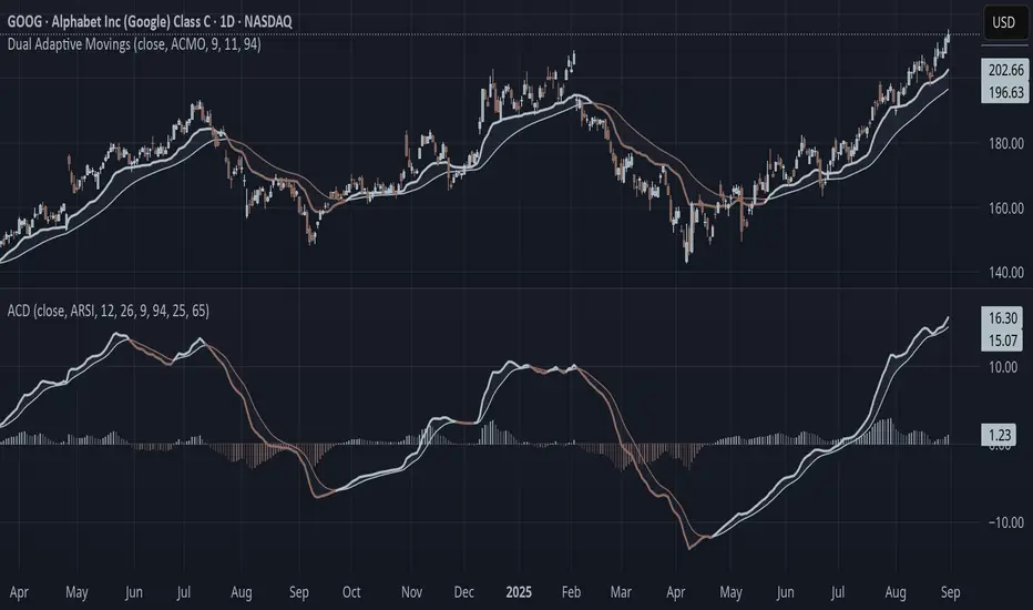
Adaptive Convergence Divergence### Adaptive Convergence Divergence (ACD)
By Gurjit Singh
The Adaptive Convergence Divergence (ACD) reimagines the classic MACD by replacing fixed moving averages with adaptive moving averages. Instead of a static smoothing factor, it dynamically adjusts sensitivity based on price momentum, relative strength, volatility, fractal roughness, or volume pressure. This makes the oscillator more responsive in trending markets while filtering noise in choppy ranges.
#### 📌 Key Features
1. Dual Adaptive Structure: The oscillator uses two adaptive moving averages to form its convergence-divergence line, with EMA/RMA as signal line:
* Primary Adaptive (MA): Fast line, reacts quickly to changes.
* Following Adaptive (FAMA): Slow line, with half-alpha smoothing for confirmation.
2. Adaptive MA Types
* ACMO: Adaptive CMO (momentum)
* ARSI: Adaptive RSI (relative strength)
* FRMA: Fractal Roughness (volatility + fractal dimension)
* VOLA: Volume adaptive (volume pressure)
3. PPO Option: Switch between classic MACD or Percentage Price Oscillator (PPO) style calculation.
4. Signal Smoothing: Choose between EMA or Wilder’s RMA.
5. Visuals: Colored oscillator, signal line, histogram with adaptive transparency.
6. Alerts: Bullish/Bearish crossovers built-in.
#### 🔑 How to Use
1. Add to chart: Works on any timeframe and asset.
2. Choose MA Type: Experiment with ACMO, ARSI, FRMA, or VOLA depending on market regime.
3. Crossovers:
* Bullish (🐂): Oscillator crosses above signal → potential long entry.
* Bearish (🐻): Oscillator crosses below signal → potential short entry.
4. Histogram: expansion = strengthening trend; contraction = weakening trend.
5. Divergences:
* Bullish (hidden strength): Price pushes lower, but ACD turns higher = potential upward reversal.
* Bearish (hidden weakness): Price pushes higher, but ACD turns lower = potential downward reversal.
6. Customize: Adjust lengths, smoothing type, and PPO/MACD mode to match your style.
7. Set Alerts:
* Enable Bullish or Bearish crossover alerts to catch momentum shifts in real time.
#### 💡 Tips
* PPO mode normalizes values across assets, useful for cross-asset analysis.
* Wilder’s smoothing is gentler than EMA, reducing whipsaws in sideways conditions.
* Adaptive smoothing helps reduce false divergence signals by filtering noise in choppy ranges.
Up/Down Volume Delta %this script is based on FractalTrade_'s rendition of the up/down volume bars.
the shortcomings of that chart were that large volume bars caused the auto-scaling to shrink smaller volume bar displays to the point where much of the data was too small to see.
in this chart, the bars are displaying the percent delta out of the total bar volume. this way, large overall volume bars do not cause visual compression to everything else in the chart.
I've used color modulation to indicate relation to a relative volume point, so users can still tell when overall volume is large or small. when volume is under a moving average, the bars will display at a basis transparency. when the volume is over the average, the brightness will increase up to a specific ratio of volume defined by the user.
for example, if basis transparency is at 20, and the full opacity ratio is at 3, and the volume average is at 1M, a volume of 750k will display the delta bar at the basis transparency. a volume of 3M will achieve full brightness. a volume of 2M will display with moderate brightness (about 60%), but still stand out against other bars with basis transparency.
areas of the chart that are either increasing bar sizes or increasing in brightness can indicate directional force. when volume delta direction contradicts the candle direction, this can indicate support / resistance.

Multifractal Forecast [ScorsoneEnterprises]Multifractal Forecast Indicator
The Multifractal Forecast is an indicator designed to model and forecast asset price movements using a multifractal framework. It uses concepts from fractal geometry and stochastic processes, specifically the Multifractal Model of Asset Returns (MMAR) and fractional Brownian motion (fBm), to generate price forecasts based on historical price data. The indicator visualizes potential future price paths as colored lines, providing traders with a probabilistic view of price trends over a specified trading time scale. Below is a detailed breakdown of the indicator’s functionality, inputs, calculations, and visualization.
Overview
Purpose: The indicator forecasts future price movements by simulating multiple price paths based on a multifractal model, which accounts for the complex, non-linear behavior of financial markets.
Key Concepts:
Multifractal Model of Asset Returns (MMAR): Models price movements as a multifractal process, capturing varying degrees of volatility and self-similarity across different time scales.
Fractional Brownian Motion (fBm): A generalization of Brownian motion that incorporates long-range dependence and self-similarity, controlled by the Hurst exponent.
Binomial Cascade: Used to model trading time, introducing heterogeneity in time scales to reflect market activity bursts.
Hurst Exponent: Measures the degree of long-term memory in the price series (persistence, randomness, or mean-reversion).
Rescaled Range (R/S) Analysis: Estimates the Hurst exponent to quantify the fractal nature of the price series.
Inputs
The indicator allows users to customize its behavior through several input parameters, each influencing the multifractal model and forecast generation:
Maximum Lag (max_lag):
Type: Integer
Default: 50
Minimum: 5
Purpose: Determines the maximum lag used in the rescaled range (R/S) analysis to calculate the Hurst exponent. A higher lag increases the sample size for Hurst estimation but may smooth out short-term dynamics.
2 to the n values in the Multifractal Model (n):
Type: Integer
Default: 4
Purpose: Defines the resolution of the multifractal model by setting the size of arrays used in calculations (N = 2^n). For example, n=4 results in N=16 data points. Larger n increases computational complexity and detail but may exceed Pine Script’s array size limits (capped at 100,000).
Multiplier for Binomial Cascade (m):
Type: Float
Default: 0.8
Purpose: Controls the asymmetry in the binomial cascade, which models trading time. The multiplier m (and its complement 2.0 - m) determines how mass is distributed across time scales. Values closer to 1 create more balanced cascades, while values further from 1 introduce more variability.
Length Scale for fBm (L):
Type: Float
Default: 100,000.0
Purpose: Scales the fractional Brownian motion output, affecting the amplitude of simulated price paths. Larger values increase the magnitude of forecasted price movements.
Cumulative Sum (cum):
Type: Integer (0 or 1)
Default: 1
Purpose: Toggles whether the fBm output is cumulatively summed (1=On, 0=Off). When enabled, the fBm series is accumulated to simulate a price path with memory, resembling a random walk with long-range dependence.
Trading Time Scale (T):
Type: Integer
Default: 5
Purpose: Defines the forecast horizon in bars (20 bars into the future). It also scales the binomial cascade’s output to align with the desired trading time frame.
Number of Simulations (num_simulations):
Type: Integer
Default: 5
Minimum: 1
Purpose: Specifies how many forecast paths are simulated and plotted. More simulations provide a broader range of possible price outcomes but increase computational load.
Core Calculations
The indicator combines several mathematical and statistical techniques to generate price forecasts. Below is a step-by-step explanation of its calculations:
Log Returns (lgr):
The indicator calculates log returns as math.log(close / close ) when both the current and previous close prices are positive. This measures the relative price change in a logarithmic scale, which is standard for financial time series analysis to stabilize variance.
Hurst Exponent Estimation (get_hurst_exponent):
Purpose: Estimates the Hurst exponent (H) to quantify the degree of long-term memory in the price series.
Method: Uses rescaled range (R/S) analysis:
For each lag from 2 to max_lag, the function calc_rescaled_range computes the rescaled range:
Calculate the mean of the log returns over the lag period.
Compute the cumulative deviation from the mean.
Find the range (max - min) of the cumulative deviation.
Divide the range by the standard deviation of the log returns to get the rescaled range.
The log of the rescaled range (log(R/S)) is regressed against the log of the lag (log(lag)) using the polyfit_slope function.
The slope of this regression is the Hurst exponent (H).
Interpretation:
H = 0.5: Random walk (no memory, like standard Brownian motion).
H > 0.5: Persistent behavior (trends tend to continue).
H < 0.5: Mean-reverting behavior (price tends to revert to the mean).
Fractional Brownian Motion (get_fbm):
Purpose: Generates a fractional Brownian motion series to model price movements with long-range dependence.
Inputs: n (array size 2^n), H (Hurst exponent), L (length scale), cum (cumulative sum toggle).
Method:
Computes covariance for fBm using the formula: 0.5 * (|i+1|^(2H) - 2 * |i|^(2H) + |i-1|^(2H)).
Uses Hosking’s method (referenced from Columbia University’s implementation) to generate fBm:
Initializes arrays for covariance (cov), intermediate calculations (phi, psi), and output.
Iteratively computes the fBm series by incorporating a random term scaled by the variance (v) and covariance structure.
Applies scaling based on L / N^H to adjust the amplitude.
Optionally applies cumulative summation if cum = 1 to produce a path with memory.
Output: An array of 2^n values representing the fBm series.
Binomial Cascade (get_binomial_cascade):
Purpose: Models trading time (theta) to account for non-uniform market activity (e.g., bursts of volatility).
Inputs: n (array size 2^n), m (multiplier), T (trading time scale).
Method:
Initializes an array of size 2^n with values of 1.0.
Iteratively applies a binomial cascade:
For each block (from 0 to n-1), splits the array into segments.
Randomly assigns a multiplier (m or 2.0 - m) to each segment, redistributing mass.
Normalizes the array by dividing by its sum and scales by T.
Checks for array size limits to prevent Pine Script errors.
Output: An array (theta) representing the trading time, which warps the fBm to reflect market activity.
Interpolation (interpolate_fbm):
Purpose: Maps the fBm series to the trading time scale to produce a forecast.
Method:
Computes the cumulative sum of theta and normalizes it to .
Interpolates the fBm series linearly based on the normalized trading time.
Ensures the output aligns with the trading time scale (T).
Output: An array of interpolated fBm values representing log returns over the forecast horizon.
Price Path Generation:
For each simulation (up to num_simulations):
Generates an fBm series using get_fbm.
Interpolates it with the trading time (theta) using interpolate_fbm.
Converts log returns to price levels:
Starts with the current close price.
For each step i in the forecast horizon (T), computes the price as prev_price * exp(log_return).
Output: An array of price levels for each simulation.
Visualization:
Trigger: Updates every T bars when the bar state is confirmed (barstate.isconfirmed).
Process:
Clears previous lines from line_array.
For each simulation, plots a line from the current bar’s close price to the forecasted price at bar_index + T.
Colors the line using a gradient (color.from_gradient) based on the final forecasted price relative to the minimum and maximum forecasted prices across all simulations (red for lower prices, teal for higher prices).
Output: Multiple colored lines on the chart, each representing a possible price path over the next T bars.
How It Works on the Chart
Initialization: On each bar, the indicator calculates the Hurst exponent (H) using historical log returns and prepares the trading time (theta) using the binomial cascade.
Forecast Generation: Every T bars, it generates num_simulations price paths:
Each path starts at the current close price.
Uses fBm to model log returns, warped by the trading time.
Converts log returns to price levels.
Plotting: Draws lines from the current bar to the forecasted price T bars ahead, with colors indicating relative price levels.
Dynamic Updates: The forecast updates every T bars, replacing old lines with new ones based on the latest price data and calculations.
Key Features
Multifractal Modeling: Captures complex market dynamics by combining fBm (long-range dependence) with a binomial cascade (non-uniform time).
Customizable Parameters: Allows users to adjust the forecast horizon, model resolution, scaling, and number of simulations.
Probabilistic Forecast: Multiple simulations provide a range of possible price outcomes, helping traders assess uncertainty.
Visual Clarity: Gradient-colored lines make it easy to distinguish bullish (teal) and bearish (red) forecasts.
Potential Use Cases
Trend Analysis: Identify potential price trends or reversals based on the direction and spread of forecast lines.
Risk Assessment: Evaluate the range of possible price outcomes to gauge market uncertainty.
Volatility Analysis: The Hurst exponent and binomial cascade provide insights into market persistence and volatility clustering.
Limitations
Computational Intensity: Large values of n or num_simulations may slow down execution or hit Pine Script’s array size limits.
Randomness: The binomial cascade and fBm rely on random terms (math.random), which may lead to variability between runs.
Assumptions: The model assumes log-normal price movements and fractal behavior, which may not always hold in extreme market conditions.
Adjusting Inputs:
Set max_lag based on the desired depth of historical analysis.
Adjust n for model resolution (start with 4–6 to avoid performance issues).
Tune m to control trading time variability (0.5–1.5 is typical).
Set L to scale the forecast amplitude (experiment with values like 10,000–1,000,000).
Choose T based on your trading horizon (20 for short-term, 50 for longer-term for example).
Select num_simulations for the number of forecast paths (5–10 is reasonable for visualization).
Interpret Output:
Teal lines suggest bullish scenarios, red lines suggest bearish scenarios.
A wide spread of lines indicates high uncertainty; convergence suggests a stronger trend.
Monitor Updates: Forecasts update every T bars, so check the chart periodically for new projections.
Chart Examples
This is a daily AMEX:SPY chart with default settings. We see the simulations being done every T bars and they provide a range for us to analyze with a few simulations still in the range.
On this intraday PEPPERSTONE:COCOA chart I modified the Length Scale for fBm, L, parameter to be 1000 from 100000. Adjusting the parameter as you switch between timeframes can give you more contextual simulations.
On BITSTAMP:ETHUSD I modified the L to be 1000000 to have a more contextual set of simulations with crypto's volatile nature.
With L at 100000 we see the range for NASDAQ:TLT is correctly simulated. The recent pop stays within the bounds of the highest simulation. Note this is a cherry picked example to show the power and potential of these simulations.
Technical Notes
Error Handling: The script includes checks for array size limits and division by zero (math.abs(denominator) > 1e-10, v := math.max(v, 1e-10)).
External Reference: The fBm implementation is based on Hosking’s method (www.columbia.edu), ensuring a robust algorithm.
Conclusion
The Multifractal Forecast is a powerful tool for traders seeking to model complex market dynamics using a multifractal framework. By combining fBm, binomial cascades, and Hurst exponent analysis, it generates probabilistic price forecasts that account for long-range dependence and non-uniform market activity. Its customizable inputs and clear visualizations make it suitable for both technical analysis and strategy development, though users should be mindful of its computational demands and parameter sensitivity. For optimal use, experiment with input settings and validate forecasts against other technical indicators or market conditions.
Elliott Wave Noise FilterElliott Wave Noise Filter
Overview
The Elliott Wave Noise Filter is a specialized indicator for TradingView, designed to solve one of the biggest challenges in Elliott Wave analysis on lower timeframes: the identification of market noise. By combining multiple advanced filtering techniques, this indicator helps distinguish meaningful price action from random fluctuations.
The Problem
On lower timeframes—especially below 15 minutes—Elliott Wave analysis is significantly impacted by excessive market noise. This noise can lead to misinterpretation of wave structures, making it difficult to execute reliable trading decisions.
The Solution
The Elliott Wave Noise Filter utilizes four powerful methods to detect and filter noise:
ATR-Based Volatility Analysis: Identifies price movements too small to be structurally meaningful
Volume Confirmation: Filters out price moves that occur with insufficient volume
Trend Strength Measurement (ADX): Detects periods of weak trend activity, where noise tends to dominate
Fractal Pattern Recognition: Marks significant turning points that could be relevant for Elliott Wave analysis
Features
Visual Indicators
Background Coloring: Red indicates noise; green signifies a clear signal
Hull Moving Average: Smooths price action and highlights the prevailing trend
Fractal Markers: Triangles mark significant highs and lows
Status Panel: Displays current noise status and ADX value
Customization Options
ATR Period: Adjust the lookback period for ATR calculations
Noise Threshold: Defines the percentage of ATR below which a movement is considered noise
Volume Filter: Can be enabled or disabled
Volume Threshold: Sets the ratio to average volume for a move to be deemed significant
Hull MA Display and Length: Configure the moving average settings
ADX Parameters: Adjust trend strength sensitivity
Use Cases
For Elliott Wave Analysis
Eliminate noise to identify cleaner wave structures
Use fractal markers as potential wave endpoints
Reference the Hull MA for determining the broader trend
For General Trading
Identify high-noise periods to avoid low-quality setups
Spot clearer market phases for better entries
Assess price action quality through visual cues
Multi-Timeframe Approach
Apply the indicator across different timeframes for a comprehensive view
Prefer trading when both higher and lower timeframes align with consistent signals
Optimal Settings
For Very Short Timeframes (1–5 minutes)
Higher Noise Threshold (0.4–0.5)
Longer ATR Period (20–30)
Higher Volume Threshold (1.0–1.2)
For Medium Timeframes (15–60 minutes)
Medium Noise Threshold (0.2–0.3)
Standard ATR Period (14)
Standard Volume Threshold (0.8)
For Higher Timeframes (4h and above)
Lower Noise Threshold (0.1–0.2)
Shorter ATR Period (10)
Lower Volume Threshold (0.6–0.7)
Conclusion
The Elliott Wave Noise Filter is an essential tool for any Elliott Wave analyst or trader working on lower timeframes. By reducing noise and emphasizing significant market movements, it enables more precise analysis and potentially more profitable trading decisions.
Note: As with any technical indicator, the Elliott Wave Noise Filter should be used as part of a broader trading strategy and not as a standalone signal for trade execution.

Institutional Quantum Momentum Impulse [BullByte]## Overview
The Institutional Quantum Momentum Impulse (IQMI) is a sophisticated momentum oscillator designed to detect institutional-level trend strength, volatility conditions, and market regime shifts. It combines multiple advanced technical concepts, including:
- Quantum Momentum Engine (Hilbert Transform + MACD Divergence + Stochastic Energy)
- Fractal Volatility Scoring (GARCH + Keltner-based volatility)
- Dynamic Adaptive Bands (Self-adjusting thresholds based on efficiency)
- Market Phase Detection (Volume + Momentum alignment)
- Liquidity & Cumulative Delta Analysis
The indicator provides a Z-score normalized momentum reading, making it ideal for mean-reversion and trend-following strategies.
---
## Key Features
### 1. Quantum Momentum Core
- Combines Hilbert Transform, MACD divergence, and Stochastic Energy into a single composite momentum score.
- Normalized using a Z-score for statistical significance.
- Smoothed with EMA/WMA/HMA for cleaner signals.
### 2. Dynamic Adaptive Bands
- Upper/Lower bands adjust based on volatility and efficiency ratio .
- Acts as overbought/oversold zones when momentum reaches extremes.
### 3. Market Phase Detection
- Identifies bullish , bearish , or neutral phases using:
- Volume-Weighted MA alignment
- Fractal momentum extremes
### 4. Volatility & Liquidity Filters
- Fractal Volatility Score (0-100 scale) shows market instability.
- Liquidity Check ensures trades are taken in favorable spread conditions.
### 5. Dashboard & Visuals
- Real-time dashboard with key metrics:
- Momentum strength, volatility, efficiency, cumulative delta, and market regime.
- Gradient coloring for intuitive momentum visualization .
---
## Best Trade Setups
### 1. Trend-Following Entries
- Signal :
- QM crosses above zero + Market Phase = Bullish + ADX > 25
- Cumulative Delta rising (buying pressure)
- Confirmation :
- Efficiency > 0.5 (strong momentum quality)
- Liquidity = High (tight spreads)
### 2. Mean-Reversion Entries
- Signal :
- QM touches upper band + Volatility expanding
- Market Regime = Ranging (ADX < 25)
- Confirmation :
- Efficiency < 0.3 (weak momentum follow-through)
- Cumulative Delta divergence (price high but delta declining)
### 3. Breakout Confirmation
- Signal :
- QM holds above zero after a pullback
- Market Phase shifts to Bullish/Bearish
- Confirmation :
- Volatility rising (expansion phase)
- Liquidity remains high
---
## Recommended Timeframes
- Intraday (5M - 1H): Works well for scalping & swing trades.
- Swing Trading (4H - Daily): Best for trend-following setups.
- Position Trading (Weekly+): Useful for macro trend confirmation.
---
## Input Customization
- Resonance Factor (1.0 - 3.618 ): Adjusts MACD divergence sensitivity.
- Entropy Filter (0.382/0.50/0.618) : Controls stochastic damping.
- Smoothing Type (EMA/WMA/HMA) : Changes momentum responsiveness.
- Normalization Period : Adjusts Z-score lookback.
---
The IQMI is a professional-grade momentum indicator that combines institutional-level concepts into a single, easy-to-read oscillator. It works across all markets (stocks, forex, crypto) and is ideal for traders who want:
✅ Early trend detection
✅ Volatility-adjusted signals
✅ Institutional liquidity insights
✅ Clear dashboard for quick analysis
Try it on TradingView and enhance your trading edge! 🚀
Happy Trading!
- BullByte
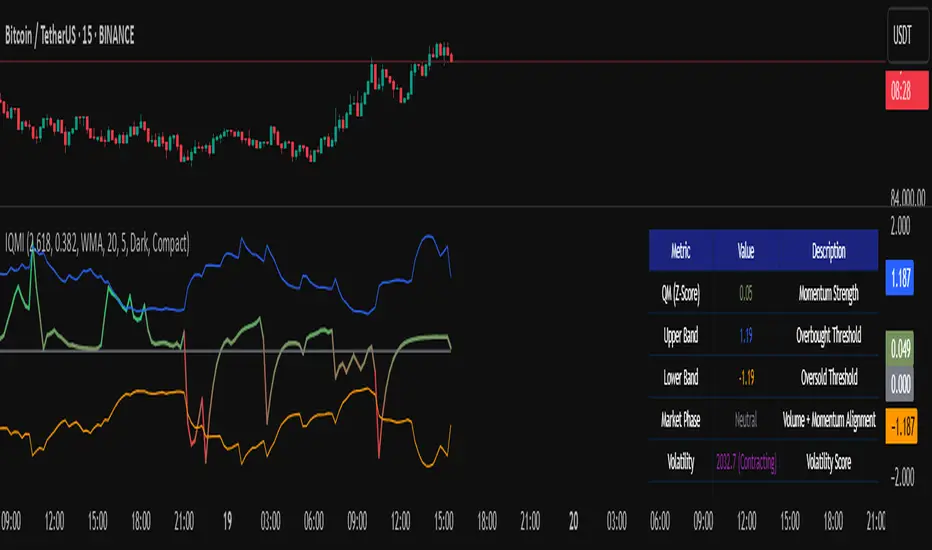
Adaptive Stochastic Oscillator with Signals [AIBitcoinTrend]👽 Adaptive Stochastic Oscillator with Signals (AIBitcoinTrend)
The Adaptive Stochastic Oscillator with Signals is a refined version of the traditional Stochastic Oscillator, dynamically adjusting its lookback period based on market volatility. This adaptive approach improves responsiveness to market conditions, reducing lag while maintaining trend sensitivity. Additionally, the indicator includes real-time divergence detection and an ATR-based trailing stop system, allowing traders to manage risk and optimize trade exits effectively.
👽 What Makes the Adaptive Stochastic Oscillator Unique?
Unlike the standard Stochastic Oscillator, which uses a fixed lookback period, this version dynamically adjusts the period length using an ATR-based fractal dimension. This makes it more responsive to market conditions, filtering out noise while capturing key price movements.
Key Features:
Adaptive Lookback Calculation – Stochastic period changes dynamically based on volatility.
Real-Time Divergence Detection – Identify bullish and bearish divergences instantly.
Implement Crossover/Crossunder signals tied to ATR-based trailing stops for risk management
👽 The Math Behind the Indicator
👾 Adaptive Lookback Period Calculation
Traditional Stochastic Oscillators use a fixed-length period for their calculations, which can lead to inaccurate signals in varying market conditions. This version automatically adjusts its lookback period based on market volatility using an ATR-based fractal dimension approach.
How it Works:
The fractal dimension (FD) is calculated using the ATR (Average True Range) over a defined period.
FD values dynamically adjust the Stochastic lookback period between a minimum and maximum range.
This results in a faster response in high-volatility conditions and smoother signals during low volatility.
👽 How Traders Can Use This Indicator
👾 Divergence Trading Strategy
Traders can anticipate trend reversals before they occur using real-time divergence detection.
Bullish Divergence Setup:
Identify price making a lower low while Stochastic %K makes a higher low.
Enter a long trade when Stochastic confirms upward momentum.
Bearish Divergence Setup:
Identify price making a higher high while Stochastic %K makes a lower high.
Enter a short trade when Stochastic confirms downward momentum.
👾 Trailing Stop & Signal-Based Trading
Bullish Setup:
✅Stochastic %K crosses above 90 → Buy signal.
✅A bullish trailing stop is placed at low - ATR × Multiplier.
✅Exit if the price crosses below the stop.
Bearish Setup:
✅Stochastic %K crosses below 10 → Sell signal.
✅A bearish trailing stop is placed at high + ATR × Multiplier.
✅Exit if the price crosses above the stop.
👽 Why It’s Useful for Traders
Adaptive Period Calculation: Dynamically adjusts to market volatility.
Real-Time Divergence Alerts: Helps traders identify trend reversals in advance.
ATR-Based Risk Management: Automatically adjusts stop levels based on price movements.
Works Across Multiple Markets & Timeframes: Useful for stocks, forex, crypto, and futures trading.
👽 Indicator Settings
Min & Max Lookback Periods – Define the range for the adaptive Stochastic period.
Enable Divergence Analysis – Toggle real-time divergence detection.
Lookback Period – Set the number of bars for detecting pivot points.
Enable Trailing Stop – Activate the dynamic trailing stop feature.
ATR Multiplier – Adjust stop-loss sensitivity.
Line Width & Colors – Customize stop-loss visualization.
Disclaimer: This indicator is designed for educational purposes and does not constitute financial advice. Please consult a qualified financial advisor before making investment decisions.

FRAMA Channel [BigBeluga]This is a trend-following indicator that utilizes the Fractal Adaptive Moving Average (FRAMA) to create a dynamic channel around the price. The FRAMA Channel helps identify uptrends, downtrends, and ranging markets by examining the relationship between the price and the channel's boundaries. It also marks trend changes with arrows, optionally displaying either price values or average volume at these key points.
🔵 IDEA
The core idea behind the FRAMA Channel indicator is to use the fractal nature of markets to adapt to different market conditions. By creating a channel around the FRAMA line, it not only tracks price trends but also adapts its sensitivity based on market volatility. When the price crosses the upper or lower bands of the channel, it signals a potential shift in trend direction. If the price remains within the channel and crosses over the upper or lower bands without a breakout, the market is likely in a ranging phase with low momentum. This adaptive approach makes the FRAMA Channel effective in both trending and ranging market environments.
🔵 KEY FEATURES & USAGE
◉ Dynamic FRAMA Channel with Trend Signals:
The FRAMA Channel uses a fractal-based moving average to create an adaptive channel around the price. When the price crosses above the upper band, it signals an uptrend and plots an upward arrow with the price (or average volume) value. Conversely, when the price crosses below the lower band, it signals a downtrend and marks the point with a downward arrow. This dynamic adaptation to market conditions helps traders identify key trend shifts effectively.
◉ Ranging Market Detection:
If the price remains within the channel, and only the high crosses the upper band or the low crosses the lower band, the indicator identifies a ranging market with low momentum. In this case, the channel turns gray, signaling a neutral trend. This is particularly useful for avoiding false signals during periods of market consolidation.
◉ Color-Coded Candles and Channel Bands:
Candles and channel bands are color-coded to reflect the current trend direction. Green indicates an upward trend, blue shows a downward trend, and gray signals a neutral or ranging market. This visual representation makes it easy to identify the market condition at a glance, helping traders make informed decisions quickly.
◉ Customizable Display of Price or Average Volume:
On trend change signals, the indicator allows users to choose whether to display the price at the point of trend change or the average volume of 10 bars. This flexibility enables traders to focus on the information that is most relevant to their strategy, whether it's the exact price entery or the volume context of the market shift. Displaying the average volume allows to see the strength of the trend change.
Price Data:
Average Volume of points:
🔵 CUSTOMIZATION
Length & Bands Distance: Adjust the length for the FRAMA calculation to control the sensitivity of the channel. A shorter length makes the channel more reactive to price changes, while a longer length smooths it out. The Bands Distance setting determines how far the bands are from the FRAMA line, helping to define the breakout and ranging conditions.
Signals Data: Choose between displaying the price or the average volume on trend change arrows. This allows traders to focus on either the exact price level of trend change or the market volume context.
Color Settings: Customize the colors for upward momentum, downward momentum, and neutral states to suit your charting preferences. You can also toggle whether to color the candles based on the momentum for a clearer visual of the trend direction.
The FRAMA Channel indicator adapts to market conditions, providing a versatile tool for identifying trends and ranging markets with clear visual cues.

Sweep institutionalThis indicator focuses on identifying "SWEEPs" based on taking liquidity at highs and lows. The application of the SWEEP strategy is highly determinant in the Swing points, as they serve as the target of our operations.
ALERTS INCLUDED
🔹Example of Strategy Application
1.-Create the BULLISH SWEEP.
2.-You can enter LONG.
3.-If it is a BULLISH SWEEP, take a long with a SWING HIGH target (2-3 pips up).
4.-If it is a BULLISH SWEEP, place your SL behind the SWEEP (2-3 pips).
(This example is bullish, but it would be the same in a bearish setup, applying everything in the opposite way)
t's very crucial for the strategy to reference SWING POINTS, as these points will be our take profit and stop loss points.
The strategy is based on identifying a SWEEP. After this, we can look for trading opportunities with targets on the opposite side of the fractal. Remember, if you decide to enter, the Stop Loss should be placed protected by the Sweep, and the Take Profit should be set at the opposite Swing, as seen in the example.
Use this STRATEGY IN TIMEFRAMES GREATER THAN 30M. If you decide to use it in timeframes <30M, there's a higher probability of encountering false SWEEPs (the most optimal are 1h & 4h)
🔹Use
The Sweep strategy involves identifying potential trades based on the creation of a "SWEEP" (liquidity grab) at the Swing High or Swing Low. Below is an example of a bearish opportunity after taking liquidity from a Swing High with a wick and no candle body closing above it.
🔹Details
As you have seen, it indicates the surpassing of a high without the candle body, this is called a “SWEEP.” Each time this occurs, the price is likely to surpass the opposite SWING High/Low. The following example will show more clearly how it works in both bullish and bearish scenarios.
🔹Configuration
-Cooldown period: is the length of the operating Range line
-Swing detection: determines the points to be used as SL and TP protection
Bullish/Berish Sweep
-Line Width: size of the line
-Line Style: design type
-Color
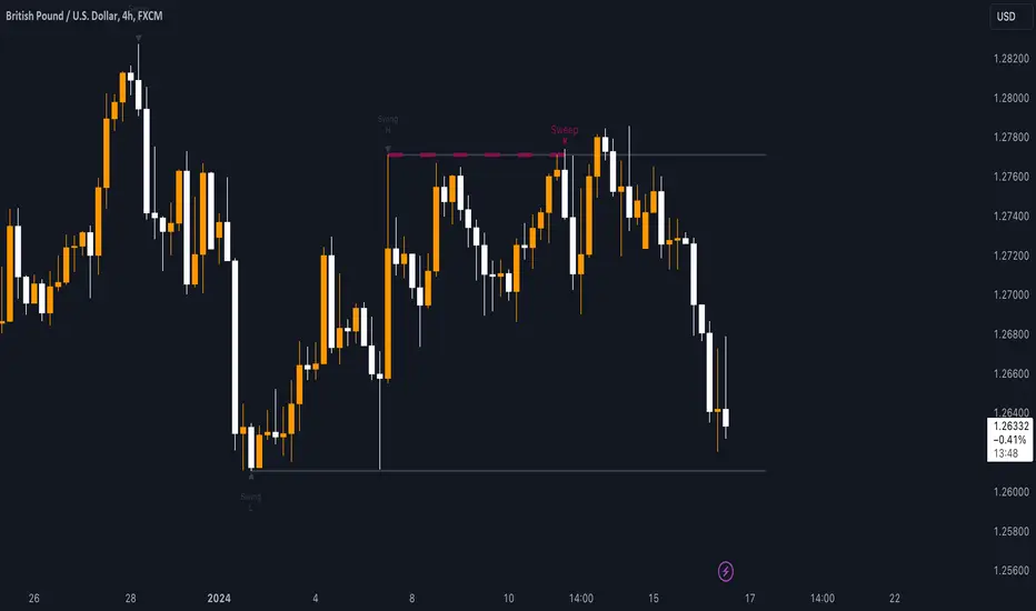
AI-Bank-Nifty Tech AnalysisThis code is a TradingView indicator that analyzes the Bank Nifty index of the Indian stock market. It uses various inputs to customize the indicator's appearance and analysis, such as enabling analysis based on the chart's timeframe, detecting bullish and bearish engulfing candles, and setting the table position and style.
The code imports an external script called BankNifty_CSM, which likely contains functions that calculate technical indicators such as the RSI, MACD, VWAP, and more. The code then defines several table cell colors and other styling parameters.
Next, the code defines a table to display the technical analysis of eight bank stocks in the Bank Nifty index. It then defines a function called get_BankComponent_Details that takes a stock symbol as input, requests the stock's OHLCV data, and calculates several technical indicators using the imported CSM_BankNifty functions.
The code also defines two functions called get_EngulfingBullish_Detection and get_EngulfingBearish_Detection to detect bullish and bearish engulfing candles.
Finally, the code calculates the technical analysis for each bank stock using the get_BankComponent_Details function and displays the results in the table. If the engulfing input is enabled, the code also checks for bullish and bearish engulfing candles and displays buy/sell signals accordingly.
The FRAMA stands for "Fractal Adaptive Moving Average," which is a type of moving average that adjusts its smoothing factor based on the fractal dimension of the price data. The fractal dimension reflects self-similarity at different scales. The FRAMA uses this property to adapt to the scale of price movements, capturing short-term and long-term trends while minimizing lag. The FRAMA was developed by John F. Ehlers and is commonly used by traders and analysts in technical analysis to identify trends and generate buy and sell signals. I tried to create this indicator in Pine.
In this context, "RS" stands for "Relative Strength," which is a technical indicator that compares the performance of a particular stock or market sector against a benchmark index.
The "Alligator" is a technical analysis tool that consists of three smoothed moving averages. Introduced by Bill Williams in his book "Trading Chaos," the three lines are called the Jaw, Teeth, and Lips of the Alligator. The Alligator indicator helps traders identify the trend direction and its strength, as well as potential entry and exit points. When the three lines are intertwined or close to each other, it indicates a range-bound market, while a divergence between them indicates a trending market. The position of the price in relation to the Alligator lines can also provide signals, such as a buy signal when the price crosses above the Alligator lines and a sell signal when the price crosses below them.
In addition to these, we have several other commonly used technical indicators, such as MACD, RSI, MFI (Money Flow Index), VWAP, EMA, and Supertrend. I used all the built-in functions for these indicators from TradingView. Thanks to the developer of this TradingView Indicator.
I also created a BankNifty Components Table and checked it on the dashboard.
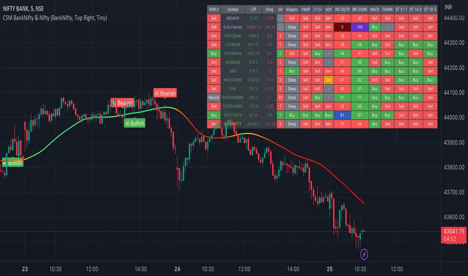
Hurst Exponent (Dubuc's variation method)Library "Hurst"
hurst(length, samples, hi, lo)
Estimate the Hurst Exponent using Dubuc's variation method
Parameters:
length : The length of the history window to use. Large values do not cause lag.
samples : The number of scale samples to take within the window. These samples are then used for regression. The minimum value is 2 but 3+ is recommended. Large values give more accurate results but suffer from a performance penalty.
hi : The high value of the series to analyze.
lo : The low value of the series to analyze.
The Hurst Exponent is a measure of fractal dimension, and in the context of time series it may be interpreted as indicating a mean-reverting market if the value is below 0.5 or a trending market if the value is above 0.5. A value of exactly 0.5 corresponds to a random walk.
There are many definitions of fractal dimension and many methods for its estimation. Approaches relying on calculation of an area, such as the Box Counting Method, are inappropriate for time series data, because the units of the x-axis (time) do match the units of the y-axis (price). Other approaches such as Detrended Fluctuation Analysis are useful for nonstationary time series but are not exactly equivalent to the Hurst Exponent.
This library implements Dubuc's variation method for estimating the Hurst Exponent. The technique is insensitive to x-axis units and is therefore useful for time series. It will give slightly different results to DFA, and the two methods should be compared to see which estimator fits your trading objectives best.
Original Paper:
Dubuc B, Quiniou JF, Roques-Carmes C, Tricot C. Evaluating the fractal dimension of profiles. Physical Review A. 1989;39(3):1500-1512. DOI: 10.1103/PhysRevA.39.1500
Review of various Hurst Exponent estimators for time-series data, including Dubuc's method:
www.intechopen.com

FDI-Adaptive Non-Lag Moving Average [Loxx]FDI-Adaptive Non-Lag Moving Average is a Fractal Dimension Index adaptive Non-Lag moving Average. This acts more like a trend coloring indictor with gradient coloring.
What is the Fractal Dimension Index?
The goal of the fractal dimension index is to determine whether the market is trending or in a trading range. It does not measure the direction of the trend. A value less than 1.5 indicates that the price series is persistent or that the market is trending. Lower values of the FDI indicate a stronger trend. A value greater than 1.5 indicates that the market is in a trading range and is acting in a more random fashion.
Included
Bar coloring
Loxx's Expanded Source Types

FDI-Adaptive, Jurik-Filtered, TMA w/ Price Zones [Loxx]FDI-Adaptive, Jurik-Filtered, TMA w/ Price Zones is a Triangular Moving Average that is Fractal Dimension Index Adaptive with Jurik Smoothing. You'll notice that this combination not only smooths out the signal but also catches bottoms better than other FIR digital filters. This is a multi-layered adaptive moving average. Price zones are calculated using a weighted range function. Future updates will included signals associated with these range bands. For now, however, these range bands serve as support and resistance, stop-loss or take profit, or indicators of market reversal.
What is the Triangular Moving Average
The Triangular Moving Average is basically a double-smoothed Simple Moving Average that gives more weight to the middle section of the data interval. The TMA has a significant lag to current prices and is not well-suited to fast moving markets. TMA = SUM ( SMA values)/ N Where N = the number of periods.
What is the Fractal Dimension Index?
The goal of the fractal dimension index is to determine whether the market is trending or in a trading range. It does not measure the direction of the trend. A value less than 1.5 indicates that the price series is persistent or that the market is trending. Lower values of the FDI indicate a stronger trend. A value greater than 1.5 indicates that the market is in a trading range and is acting in a more random fashion.
What is Jurik Volty used in the Juirk Filter?
One of the lesser known qualities of Juirk smoothing is that the Jurik smoothing process is adaptive. "Jurik Volty" (a sort of market volatility ) is what makes Jurik smoothing adaptive. The Jurik Volty calculation can be used as both a standalone indicator and to smooth other indicators that you wish to make adaptive.
What is the Jurik Moving Average?
Have you noticed how moving averages add some lag (delay) to your signals? ... especially when price gaps up or down in a big move, and you are waiting for your moving average to catch up? Wait no more! JMA eliminates this problem forever and gives you the best of both worlds: low lag and smooth lines.
Included:
Bar coloring
Signals
Alerts
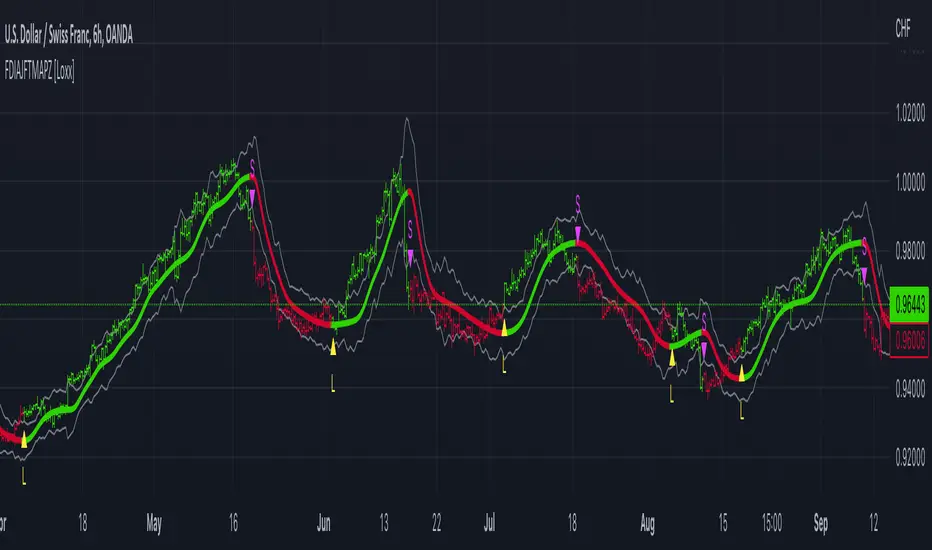
FDI-Adaptive Fisher Transform [Loxx]FDI-Adaptive Fisher Transform is a Fractal Dimension Adaptive Fisher Transform indicator.
What is the Fractal Dimension Index?
The goal of the fractal dimension index is to determine whether the market is trending or in a trading range. It does not measure the direction of the trend. A value less than 1.5 indicates that the price series is persistent or that the market is trending. Lower values of the FDI indicate a stronger trend. A value greater than 1.5 indicates that the market is in a trading range and is acting in a more random fashion.
What is Fisher Transform?
The Fisher Transform is a technical indicator created by John F. Ehlers that converts prices into a Gaussian normal distribution.
The indicator highlights when prices have moved to an extreme, based on recent prices. This may help in spotting turning points in the price of an asset. It also helps show the trend and isolate the price waves within a trend.
Included:
Zero-line and signal cross options for bar coloring
Customizable overbought/oversold thresh-holds
Alerts
Signals