Ultimate Futures Daytrade Suite v1 - The Strategy GuideHere is the complete **Strategy Guide** translated into English.
---
# 📘 Ultimate Futures Daytrade Suite – The Strategy Guide
### 1. The Visual Legend (What is what?)
Before you trade, you need to understand the hierarchy of your lines. Not every line has the same importance.
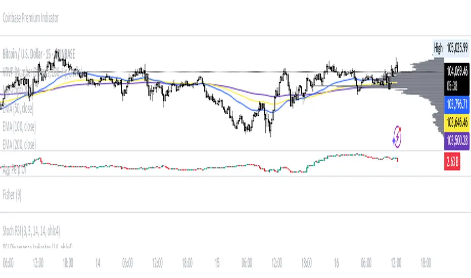
* **🟣 Daily EMA 50 (Neon Violet):** The **"Big Boss"**. It determines the **Macro Trend**.
* *Price above:* We are primarily looking for Longs.
* *Price below:* We are primarily looking for Shorts.
* **🟢 4h EMA 50 (Neon Green):** The **"Swing Trend"**. Your most important level for **Pullback Entries** (Re-entries).
* **🟡 POC (Gold) & TPO:** The **"Magnet"**. Price often returns here.
* *Rule:* Never open a trade directly *on* the POC (Risk of "Chop"). Use it as a **Target** (Take Profit).
* **🟠 IB High/Low (Orange Lines):** The **"Daily Structure"**.
* A breakout from the IB (Initial Balance) often indicates the trend direction for the day.
* **🟥/🟩 Boxes (Supply/Demand):** Resistance and Support zones from the 1h timeframe.
* **⬜ FVG Boxes:** "Gaps" in the market that are often filled.
---
### 2. The Trading Workflow (Top-Down Method)
Go through this mental checklist before every trade:
#### Step 1: Trend Check (The Traffic Light)
Look at the **Violet Line (Daily)** and the **Green Line (4h)**.
* **Bullish:** Price is above Violet AND above Green. -> *Focus: Buy dips.*
* **Bearish:** Price is below Violet AND below Green. -> *Focus: Sell rallies.*
* **Mixed:** Price is between Violet and Green. -> *Caution! Market is undecided (Range Trading).*
#### Step 2: Location (The Context)
Where is the price currently located?
* Are we at a **Green Demand Zone**?
* Are we testing the **4h EMA 50 (Green)** from above?
* Are we at the **VWAP**?
* *Never trade in "No Man's Land"!* Wait until the price touches one of your lines.
#### Step 3: Trigger (The Execution)
Now zoom into your lower timeframe (e.g., 5min or 15min).
* Wait for a reaction at the zone.
* Use the **EMA 9 (Yellow)** as a momentum trigger. If price breaks the EMA 9 and closes above/below it, that is your "Go".
---
### 3. The Setup Blueprints
Here are the two most profitable scenarios you can trade with this script:
#### A) The "Golden Trend" Setup (Long)
* **Context:** Price > **Daily EMA (Violet)**.
* **Preparation:** Price corrects (drops) back to the **4h EMA 50 (Green)** or to the **VWAP**.
* **Confluence:** Ideally, there is also a **Demand Zone (Green Box)** or an **FVG** at that level.
* **Entry:** As soon as a candle touches the zone and closes bullish again (or reclaims the EMA 9).
* **Stop-Loss:** Below the 4h EMA 50.
* **Take-Profit:** Next **Supply Zone (Red)** or the **IB High (Orange)**.
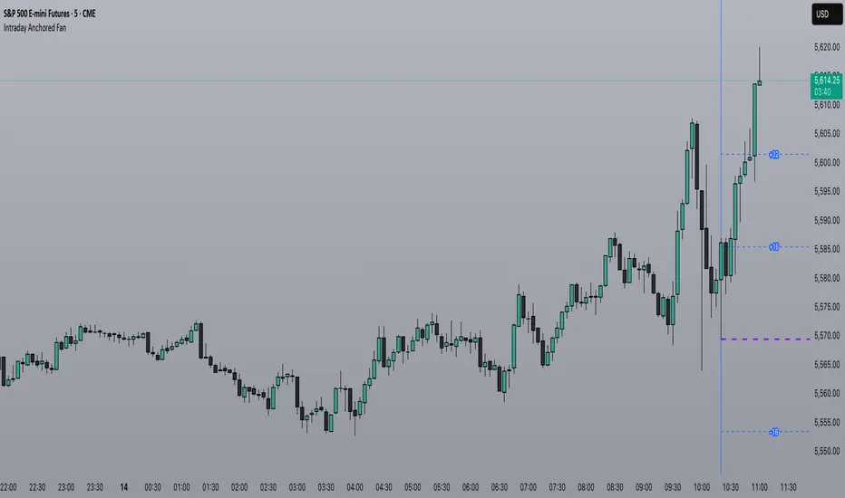
#### B) The "Daytrade Breakout" (Intraday)
* **Context:** Price opens inside yesterday's Value Area.
* **Signal:** Price breaks through the **IB High (Orange)** with momentum.
* **Filter:** Price must be above the **VWAP**.
* **Entry:** On the retest of the IB High or directly on the breakout.
* **Target:** Price often trends in that direction for the rest of the day.
---
### 4. Warning Signals (When NOT to trade)
1. **The "Concrete Ceiling":** If you want to go Long, but the **Violet Daily EMA 50** is running directly above you. This is massive resistance. Better wait until it is broken.
2. **The "POC Dance":** If price is dancing sideways around the **Gold Line (POC)**. This is a "No-Trade Zone". Day traders lose the most money here due to fees and whipsaws.
3. **Overextension:** If price is extremely far away from the **4h EMA 50 (Green)** (Rubber Band Effect). Do not enter in the trend direction here; wait for a pullback to the line.
### Summary
Your chart is now telling you a story:
* **Violet** tells you the Direction.
* **Green** gives you the Entry.
* **Red/Green Boxes** show you the Obstacles.
* **Yellow (EMA 9)** gives you the Timing.
Good luck with the Suite! This is a setup similar to what institutional traders use.
Pine Script® indicator