Buffett Quality Score [Consumer Discretionary]Evaluating Consumer Discretionary Companies with the Buffett Quality Score
The consumer discretionary sector, characterized by its sensitivity to economic cycles and consumer spending patterns, demands a robust framework for financial evaluation. The Buffett Quality Score offers a comprehensive assessment of financial health and performance specifically tailored to this dynamic industry. This scoring system combines critical financial ratios uniquely relevant to consumer discretionary companies, providing investors and analysts with a reliable tool for evaluation.
Selected Financial Metrics and Criteria
1. Altman Z-Score > 2.0
Relevance: The Altman Z-Score assesses bankruptcy risk, combining profitability, leverage, liquidity, solvency, and activity ratios. For consumer discretionary companies, which often face volatile market conditions, a score above 2.0 indicates financial stability and the ability to withstand economic downturns. This metric is particularly important in this sector due to the high variability in consumer spending.
2. Piotroski F-Score > 6.0
Relevance: The Piotroski F-Score evaluates fundamental strength based on profitability, leverage, liquidity, and operating efficiency. In the consumer discretionary sector, where rapid changes in consumer preferences can impact performance, a score above 6.0 highlights strong fundamental performance and resilience. This score is crucial for identifying companies with robust financial foundations in a highly competitive environment.
3. Asset Turnover > 1.0
Relevance: Asset Turnover measures the efficiency of asset use in generating sales. For consumer discretionary companies, a ratio above 1.0 signifies effective utilization of assets to drive revenue growth. Given the sector's reliance on high sales volumes and rapid inventory turnover, this metric is key to assessing operational efficiency.
4. Current Ratio > 1.5
Relevance: The Current Ratio assesses liquidity by comparing current assets to current liabilities. A ratio above 1.5 ensures that consumer discretionary companies can meet short-term obligations. This liquidity is essential for maintaining operational stability and flexibility to adapt to market changes, especially during economic fluctuations.
5. Debt to Equity Ratio < 1.0
Relevance: A lower Debt to Equity Ratio indicates prudent financial management and reduced reliance on debt. This is particularly important for consumer discretionary companies, which need to maintain financial flexibility to invest in new trends and innovations without overleveraging. Lower debt levels also reduce risk during economic downturns.
6. EBITDA Margin > 15.0%
Relevance: The EBITDA Margin measures operating profitability. A margin above 15.0% indicates efficient operations and the ability to generate sufficient earnings before interest, taxes, depreciation, and amortization. This is crucial for sustaining profitability in a competitive and fluctuating market, ensuring the company can reinvest in growth and innovation.
7. EPS One-Year Growth > 5.0%
Relevance: EPS growth reflects the company’s ability to increase earnings per share over the past year. For consumer discretionary companies, growth exceeding 5.0% signals positive earnings momentum, which is vital for investor confidence and the ability to fund future growth initiatives. This metric highlights companies that are successfully increasing profitability.
8. Gross Margin > 25.0%
Relevance: Gross Margin represents the profitability of sales after production costs. A margin exceeding 25.0% indicates strong pricing power and effective cost management, crucial for maintaining profitability while adapting to changing consumer demands. High gross margins are indicative of a company’s ability to control costs and price products competitively.
9. Net Margin > 10.0%
Relevance: Net Margin measures overall profitability after all expenses. A margin above 10.0% highlights the company’s ability to maintain strong profit levels, ensuring financial health and stability. This is essential for sustaining operations and investing in new opportunities, reflecting the company's efficiency in converting revenue into actual profit.
10.Return on Equity (ROE) > 15.0%
Relevance: ROE indicates how effectively a company uses equity to generate profits. An ROE above 15.0% signifies strong shareholder value creation. This metric is key for evaluating long-term performance in the consumer discretionary sector, where investor returns are closely tied to the company’s ability to innovate and grow. High ROE demonstrates effective management and profitable use of equity capital.
Interpreting the Buffett Quality Score
0-4 Points: Indicates potential weaknesses across multiple financial areas, warranting further investigation and risk assessment.
5 Points: Suggests average performance based on sector-specific criteria, indicating a need for cautious optimism.
6-10 Points: Signifies strong financial health and quality, meeting or exceeding most performance thresholds, making the company a potentially attractive investment.
Conclusion
The Buffett Quality Score provides a structured approach to evaluating financial health and performance. By focusing on these essential financial metrics, stakeholders can make informed decisions, identifying companies that are well-positioned to thrive in the competitive and economically sensitive consumer discretionary sector.
Disclaimer: The Buffett Quality Score serves as a tool for financial evaluation and analysis. It is not a substitute for professional financial advice or investment recommendations. Investors should conduct thorough research and seek personalized guidance based on individual circumstances.
Search in scripts for "profit"

Autoback Grid Lab [trade_lexx]Autoback Grid Lab: Your personal laboratory for optimizing grid strategies.
Introduction
First of all, it is important to understand that Autoback Grid Lab is a powerful professional tool for backtesting and optimization, created specifically for traders using both grid strategies and regular take profit with stop loss.
The main purpose of this script is to save you weeks and months of manual testing and parameter selection. Instead of manually testing one combination of settings after another, Autoback Grid Lab automatically tests thousands of unique strategies on historical data, providing you with a comprehensive report on the most profitable and, more importantly, sustainable ones.
If you want to find mathematically sound, most effective settings for your grid strategy on a specific asset and timeframe, then this tool was created for you.
Key Features
My tool has functionality that transforms the process of finding the perfect strategy from a routine into an exciting exploration.
🧪 Mass testing of thousands of combinations
The script is able to systematically generate and run a huge number of unique combinations of parameters through the built-in simulator. You set the ranges, and the indicator does all the work, testing all possible options for the following grid settings:
* Number of safety orders (SO Count)
* Grid step (SO Step)
* Step Multiplier (SO Multiplier) for building nonlinear grids
* Martingale for controlling the volume of subsequent orders
* Take Profit (%)
* Stop Loss (%), with the possibility of calculating both from the entry point and from the dynamic breakeven line
* The volume of the base order (Volume BO) as a percentage of the deposit
🏆 Unique `FinalScore` rating system
Sorting strategies by net profit alone is a direct path to self—deception and choosing strategies that are "tailored" to history and will inevitably fail in real trading. To solve this problem, we have developed FinalScore, a comprehensive assessment of the sustainability and quality of the strategy.
How does it work?
FinalScore analyzes each combination not one by one, but by nine key performance metrics at once, including Net Profit, Drawdown, Profit Factor, WinRate, Sharpe coefficients, Sortino, Squid and Omega. Each of these indicators is normalized, that is, reduced to a single scale. Then, to test the strategy for strength, the system performs 30 iterations, each time assigning random weights to these 9 metrics. A strategy gets a high FinalScore only if it shows consistently high results under different evaluation criteria. This proves her reliability and reduces the likelihood that her success was an accident.
📈 Realistic backtesting engine
The test results are meaningless if they do not take into account the actual trading conditions. Our simulator simulates real trading as accurately as possible, taking into account:
* Leverage: Calculation of the required margin to open and hold positions.
* Commission: A percentage commission is charged each time an order is opened and closed.
* Slippage: The order execution price is adjusted by a set percentage to simulate real market conditions.
* Liquidation model: This is one of the most important functions. The script continuously monitors the equity of the account (capital + unrealized P&L). If equity falls below the level of the supporting margin (calculated from the current value of the position), the simulator forcibly closes the position, as it would happen on a real exchange. This eliminates unrealistic scenarios where the strategy survives after a huge drawdown.
🔌 Integration with external signals
The indicator operates in two modes:
1. `No Signal': Standard mode. The trading cycle starts immediately as soon as the previous one has been closed. Ideal for testing the "pure" mechanics of the grid.
2. `External Signal`: In this mode, a new trading cycle will start only when a signal is received from an external source. You can connect any other indicator (such as the RSI, MACD, or your own strategy) to the script and use it as a trigger to log in. This allows you to combine the power of a grid strategy with your own entry points.
📊 Interactive and informative results panel
Upon completion of the calculations, a detailed table with the TOP N best strategies appears on the screen, sorted according to your chosen criterion. For each strategy in the rating, you will see not only the key metrics (Profit, Drawdown, duration of transactions), but also all the parameters that led to this result. You can immediately take these settings and apply them in your trading.
Application Options: How To Solve Your Problems
Autoback Grid Lab is a flexible tool that can be adapted to solve various tasks, from complete grid optimization to fine—tuning existing strategies. Here are some key scenarios for its use:
1. Complete Optimization Of The Grid Strategy
This is the basic and most powerful mode of use. You can find the most efficient grid configuration for any asset from scratch.
* How to use: Set wide ranges for all key grid parameters ('SO Count`, SO Step, SO Multiplier, Martingale, TP, etc.).
* In the `No Signal` mode: You will find the most stable grid configuration that works as an independent, constantly active strategy, regardless of which-or entrance indicators.
* In the `External Signal` mode: You can connect your favorite indicator for input (for example, RSI, MACD or a complex author's script) and find the optimal grid parameters that best complement your input signals. This allows you to turn a simple signaling strategy into a full-fledged grid system.
2. Selecting the Optimal Take Profit and Stop Loss for Your Strategy
Do you already have an entry strategy, but you are not sure where it is best to put Take Profit and Stop Loss? Autoback Grid Lab can solve this problem as well.
* How to use:
1. Disable optimization of all grid parameters (uncheck SO Count, SO Step, Martingale, etc.). Set the Min value for SO Count to 0.
2. Set the ranges for iteration only for 'Take Profit` and `Stop Loss'.
3. Turn on the External Signal mode and connect your indicator with input signals.
* Result: The script will run your historical entry signals with hundreds of different TP and SL combinations and show you which stop order levels bring maximum profit with minimal risk specifically for your entry points.
3. Building a Secure Network with Risk Management
Many traders are afraid of grid strategies because of the risk of large drawdowns. With the help of the optimizer, you can purposefully find the parameters for such a grid, which includes mandatory risk management through Stop Loss.
* How to use: Enable and set the range for Stop Loss, along with other grid parameters. Don't forget to test both types of SL calculations (`From entry point` and `From breakeven line`) to determine which one works more efficiently.
* Result: You will find balanced strategies in which the grid parameters (number of orders, martingale) and the Stop Loss level are selected in such a way as to maximize profits without going beyond the acceptable risk level for you.
How To Use The Indicator (Step-By-Step Guide)
Working with the Autoback Grid Lab is a sequential process consisting of four main steps: from initial setup to analysis of the finished results. Follow this guide to get the most out of the tool.
Step 1: Initial Setup
1. Add the indicator to the chart of your chosen asset and timeframe.
2. Open the script settings. The first thing you should pay attention to is the ⚙️ Optimization Settings ⚙️ group.
3. Set the `Bars Count'. This parameter determines how much historical data will be used for testing.
* Important: The more bars you specify, the more statistically reliable the backtest results will be. We recommend using the maximum available value (25,000) to test strategies at different market phases.
* Consider: The indicator performs all calculations on the last historical bar. After applying the TradingView settings, it will take some time to load all the specified bars. The results table will appear only after the data is fully loaded. Don't worry if it doesn't appear instantly. And if an error occurs, simply switch the number of combinations to 990 and back to 1000 until the table appears.
Step 2: Optimization Configuration
At this stage, you define the "universe" of parameters that our algorithm will explore.
1. Set the search ranges (🛠 Optimization Parameters 🛠 group).
For each grid parameter that you want to optimize (for example, SO Count or `Take Profit'), you must specify three values:
* Min: The minimum value of the range.
* Max: The maximum value of the range.
* Step: The step with which the values from Min to Max will be traversed.
*Example:* If you set Min=5, Max=10, and Step=1 for SO Count, the script will test strategies with 5, 6, 7, 8, 9, and 10 safety orders.
* Tip for users: To get the first results quickly, start with a larger step (for example, TP from 0.5% to 2.5% in 0.5 increments instead of 0.1). After you identify the most promising areas, you can perform a deeper analysis by expanding the ranges around these values.
2. Set Up Money Management (Group `💰 Money Management Settings 💰`).
Fill in these fields with the values that best match your actual trading conditions. This is critically important for obtaining reliable results.
* Capital: Your initial deposit.
* Leverage: Leverage.
* Commission (%): Your trading commission as a percentage.
* Slippage (%): Expected slippage.
* Liquidation Level (%): The level of the supporting margin (MMR in %). For example, for Binance Futures, this value is usually between 0.4% and 2.5%, depending on the asset and position size. Specify this value for your exchange.
3. Select the Sorting Criterion and the Direction (Group `⚙️ Optimization Settings ⚙️').
* `Sort by': Specify the main criteria by which the best strategies will be selected and sorted. I strongly recommend using finalScore to find the most balanced and sustainable strategies.
* `Direction': Choose which trades to test: Long, Short or Both.
Step 3: Start Testing and Work with "Parts"
The total number of unique combinations generated based on your ranges can reach tens of millions. TradingView has technical limitations on the number of calculations that the script can perform at a time. To get around this, I implemented a "Parts" system.
1. What are `Part` and `Combinations in Part'?
* `Combinations in Part': This is the number of backtests that the script performs in one run (1000 by default).
* `Part`: This is the number of the "portion" of combinations that you want to test.
2. How does it work in practice?
* After you have everything set up, leave Part:1 and wait for the results table to appear. You will see the TOP N best strategies from the first thousand tested.
* Analyze them. Then, to check the next thousand combinations, just change the Part to 2 in the settings and click OK. The script will run a test for the next batch.
* Repeat this process by increasing the Part number (`3`, 4, 5...), until you reach the last available part.
* Where can I see the total number of parts? In the information row below the results table, you will find Total parts. This will help you figure out how many more tests are left to run.
Step 4: Analyze the Results in the Table
The results table is your main decision—making tool. It displays the best strategies found, sorted by the criteria you have chosen.
1. Study the performance metrics:
* Rating: Position in the rating.
* Profit %: Net profit as a percentage of the initial capital.
* Drawdown%: The maximum drawdown of the deposit for the entire test period.
* Max Length: The maximum duration of one transaction in days, hours and minutes.
* Trades: The total number of completed trades.
2. Examine the winning parameters:
* To the right of the performance metrics are columns showing the exact settings that led to this result ('SO Count`, SO Step, TP (%), etc.).
3. How to choose the best strategy?
* Don't chase after the maximum profit! The strategy with the highest profit often has the highest drawdown, which makes it extremely risky.
* Seek a balance. The ideal strategy is a compromise between high profitability, low drawdown (Drawdown) and the maximum length of trades acceptable to you (Max Length).
* finalScore was created to find this balance. Trust him — he often highlights not the most profitable, but the most stable and reliable options.
Detailed Description Of The Settings
This section serves as a complete reference for each parameter available in the script settings. The parameters are grouped in the same way as in the indicator interface for your convenience.
Group: ⚙️ Optimization Settings ⚙️
The main parameters governing the testing process are collected here.
* `Enable Optimizer': The main switch. Activates or deactivates all backtesting functionality.
* `Direction': Determines which way trades will be opened during the simulation.
* Long: Shopping only.
* Short: Sales only.
* Both: Testing in both directions. Important: This mode only works in conjunction with an External Signal, as the script needs an external signal to determine the direction for each specific transaction.
* `Signal Mode`: Controls the conditions for starting a new trading cycle (opening a base order).
* No Signal: A new cycle starts immediately after the previous one is completed. This mode is used to test "pure" grid mechanics without reference to market conditions.
* External Signal: A new cycle begins only when a signal is received from an external indicator connected via the Signal field.
* `Signal': A field for connecting an external signal source (works only in the `External Signal` mode). You can select any other indicator on the chart.
* For Long** trades, the signal is considered received if the value of the external indicator ** is greater than 0.
* For Short** trades, the signal is considered received if the value of the external indicator ** is less than 0.
* `Bars Count': Sets the depth of the history in the bars for the backtest. The maximum value (25000) provides the most reliable results.
* `Sort by`: A key criterion for selecting and ranking the best strategies in the final table.
* FinalScore: Recommended mode. A comprehensive assessment that takes into account 9 metrics to find the most balanced and sustainable strategies.
* Profit: Sort by net profit.
* Drawdown: Sort by minimum drawdown.
* Max Length: Sort by the minimum length of the longest transaction.
* `Combinations Count': Indicates how many of the best strategies (from 1 to 50) will be displayed in the results table.
* `Close last trade`: If this option is enabled, any active trade will be forcibly closed at the closing price of the last historical bar. For grid strategies, it is recommended to always enable this option in order to get the correct calculation of the final profit and eliminate grid strategies that have been stuck for a long time.
Group: 💰 Money Management Settings 💰
The parameters in this group determine the financial conditions of the simulation. Specify values that are as close as possible to your actual values in order to get reliable results.
* `Capital': The initial deposit amount for the simulation.
* `Leverage`: The leverage used to calculate the margin.
* `Slippage` (%): Simulates the difference between the expected and actual order execution price. The specified percentage will be applied to each transaction.
* `Commission` (%): The trading commission of your exchange as a percentage. It is charged at the execution of each order (both at opening and closing).
* `Liquidation Level' (%): Maintenance Margin Ratio. This is a critical parameter for a realistic test. Liquidation in the simulator occurs if the Equity of the account (Capital + Unrealized P&L) falls below the level of the supporting margin.
Group: 🛠 Optimization Parameters 🛠
This is the "heart" of the optimizer, where you set ranges for iterating through the grid parameters.
* `Part`: The portion number of the combinations to be tested. Start with 1, and then increment (`2`, 3, ...) sequentially to check all generated strategies.
* `Combinations in Part': The number of backtests performed at a time (in one "Part"). Increasing the value may speed up the process, but it may cause the script to error due to platform limitations. If an error occurs, it is recommended to switch to the step below and back.
Three fields are available for each of the following parameters (`SO Count`, SO Step, SO Multiplier, etc.):
* `Min`: Minimum value for testing.
* `Max': The maximum value for testing.
* `Step`: The step with which the values in the range from Min to Max will be iterated over.
There is also a checkbox for each parameter. If it is enabled, the parameter will be optimized in the specified range. If disabled, only one value specified in the Min field will be used for all tests.
* 'Stop Loss': In addition to the standard settings Min, Max, Step, it has an additional parameter:
* `Type`: Defines how the stop loss price is calculated.
* From entry point: The SL level is calculated once from the entry price (base order price).
* From breakeven line: The SL level is dynamically recalculated from the average position price after each new safety order is executed.
Group: ⚡️Filters⚡️
Filters allow you to filter out those results from the final table that do not meet your minimum requirements.
For each filter (`Max Profit`, Min Drawdown, `Min Trade Length`), you can:
1. Turn it on or off using the checkbox.
2. Select the comparison condition: Greater (More) or Less (Less).
3. Set a threshold value.
*Example:* If you set Less and 20 for the Min Drawdown filter, only those strategies with a maximum drawdown of less than 20% will be included in the final table.
Group: 🎨 Visual Settings 🎨
Here you can customize the appearance of the results table.
* `Position': Selects the position of the table on the screen (for example, Bottom Left — bottom left).
* `Font Size': The size of the text in the table.
* `Header Background / Data Background`: Background colors for the header and data cells.
* `Header Font Color / Data Font Color`: Text colors for the header and data cells.
Important Notes and Limitations
So that you can use the Autoback Grid Lab as efficiently and consciously as possible, please familiarize yourself with the following key features of its work.
1. It is a Tool for Analysis, not for Signals
It is extremely important to understand that this script does not generate trading signals in real time. Its sole purpose is to conduct in—depth research (**backtesting**) on historical data.
* The results you see in the table are a report on how a particular strategy would have worked in the past.
* The script does not provide alerts and does not draw entry/exit points on the chart for the current market situation.
* Your task is to take the best sets of parameters found during optimization and use them in your real trading, for example, when setting up a trading bot or in a manual trading system.
2. Features Of Calculations (This is not a "Repainting")
You will notice that the results table appears and is updated only once — when all historical bars on the chart are loaded. It does not change in real time with each tick of the price.
This is correct and intentional behavior.:
* To test thousands, and sometimes millions of combinations, the script needs to perform a huge amount of calculations. In the Pine Script™ environment, it is technically possible to do this only once, at the very last bar in history.
* The script does not show false historical signals, which then disappear or change. It provides a static report on the results of the simulation, which remains unchanged for a specific historical period.
3. Past Results do not Guarantee Future Results.
This is the golden rule of trading, and it fully applies to the results of backtesting. Successful strategy performance in the past is not a guarantee that it will be as profitable in the future. Market conditions, volatility and trends are constantly changing.
My tool, especially when sorting by finalScore, is aimed at finding statistically stable and reliable strategies to increase the likelihood of their success in the future. However, it is a tool for managing probabilities, not a crystal ball for predicting the future. Always use proper risk management.
4. Dependence on the Quality and Depth of the Story
The reliability of the results directly depends on the quantity and quality of the historical data on which the test was conducted.
* Always strive to use the maximum number of bars available (`Bars Count: 25,000`) so that your strategy is tested on different market cycles (rise, fall, flat).
* The results obtained on data for one month may differ dramatically from the results obtained on data for two years. The longer the testing period, the higher the confidence in the parameters found.
Conclusion
The Autoback Grid Lab is your personal research laboratory, designed to replace intuitive guesses and endless manual selection of settings with a systematic, data—driven approach. Experiment with different assets, timeframes, and settings ranges to find the unique combinations that best suit your trading style.

Quantify [Entry Model] | FractalystWhat’s the indicator’s purpose and functionality?
Quantify is a machine learning entry model designed to help traders identify high-probability setups to refine their strategies.
➙ Simply pick your bias, select your entry timeframes, and let Quantify handle the rest for you.
Can the indicator be applied to any market approach/trading strategy?
Absolutely, all trading strategies share one fundamental element: Directional Bias
Once you’ve determined the market bias using your own personal approach, whether it’s through technical analysis or fundamental analysis, select the trend direction in the Quantify user inputs.
The algorithm will then adjust its calculations to provide optimal entry levels aligned with your chosen bias. This involves analyzing historical patterns to identify setups with the highest potential expected values, ensuring your setups are aligned with the selected direction.
Can the indicator be used for different timeframes or trading styles?
Yes, regardless of the timeframe you’d like to take your entries, the indicator adapts to your trading style.
Whether you’re a swing trader, scalper, or even a position trader, the algorithm dynamically evaluates market conditions across your chosen timeframe.
How can this indicator help me to refine my trading strategy?
1. Focus on Positive Expected Value
• The indicator evaluates every setup to ensure it has a positive expected value, helping you focus only on trades that statistically favor long-term profitability.
2. Adapt to Market Conditions
• By analyzing real-time market behavior and historical patterns, the algorithm adjusts its calculations to match current conditions, keeping your strategy relevant and adaptable.
3. Eliminate Emotional Bias
• With clear probabilities, expected values, and data-driven insights, the indicator removes guesswork and helps you avoid emotional decisions that can damage your edge.
4. Optimize Entry Levels
• The indicator identifies optimal entry levels based on your selected bias and timeframes, improving robustness in your trades.
5. Enhance Risk Management
• Using tools like the Kelly Criterion, the indicator suggests optimal position sizes and risk levels, ensuring that your strategy maintains consistency and discipline.
6. Avoid Overtrading
• By highlighting only high-potential setups, the indicator keeps you focused on quality over quantity, helping you refine your strategy and avoid unnecessary losses.
How can I get started to use the indicator for my entries?
1. Set Your Market Bias
• Determine whether the market trend is Bullish or Bearish using your own approach.
• Select the corresponding bias in the indicator’s user inputs to align it with your analysis.
2. Choose Your Entry Timeframes
• Specify the timeframes you want to focus on for trade entries.
• The indicator will dynamically analyze these timeframes to provide optimal setups.
3. Let the Algorithm Analyze
• Quantify evaluates historical data and real-time price action to calculate probabilities and expected values.
• It highlights setups with the highest potential based on your selected bias and timeframes.
4. Refine Your Entries
• Use the insights provided—entry levels, probabilities, and risk calculations—to align your trades with a math-driven edge.
• Avoid overtrading by focusing only on setups with positive expected value.
5. Adapt to Market Conditions
• The indicator continuously adapts to real-time market behavior, ensuring its recommendations stay relevant and precise as conditions change.
How does the indicator calculate the current range?
The indicator calculates the current range by analyzing swing points from the very first bar on your charts to the latest available bar it identifies external liquidity levels, also known as BSLQ (buy-side liquidity levels) and SSLQ (sell-side liquidity levels).
What's the purpose of these levels? What are the underlying calculations?
1. Understanding Swing highs and Swing Lows
Swing High: A Swing High is formed when there is a high with 2 lower highs to the left and right.
Swing Low: A Swing Low is formed when there is a low with 2 higher lows to the left and right.
2. Understanding the purpose and the underlying calculations behind Buyside, Sellside and Pivot levels.
3. Identifying Discount and Premium Zones.
4. Importance of Risk-Reward in Premium and Discount Ranges
How does the script calculate probabilities?
The script calculates the probability of each liquidity level individually. Here's the breakdown:
1. Upon the formation of a new range, the script waits for the price to reach and tap into pivot level level. Status: "■" - Inactive
2. Once pivot level is tapped into, the pivot status becomes activated and it waits for either liquidity side to be hit. Status: "▶" - Active
3. If the buyside liquidity is hit, the script adds to the count of successful buyside liquidity occurrences. Similarly, if the sellside is tapped, it records successful sellside liquidity occurrences.
4. Finally, the number of successful occurrences for each side is divided by the overall count individually to calculate the range probabilities.
Note: The calculations are performed independently for each directional range. A range is considered bearish if the previous breakout was through a sellside liquidity. Conversely, a range is considered bullish if the most recent breakout was through a buyside liquidity.
What does the multi-timeframe functionality offer?
You can incorporate up to 4 higher timeframe probabilities directly into the table.
This feature allows you to analyze the probabilities of buyside and sellside liquidity across multiple timeframes, without the need to manually switch between them.
By viewing these higher timeframe probabilities in one place, traders can spot larger market trends and refine their entries and exits with a better understanding of the overall market context.
What are the multi-timeframe underlying calculations?
The script uses the same calculations (mentioned above) and uses security function to request the data such as price levels, bar time, probabilities and booleans from the user-input timeframe.
How does the Indicator Identifies Positive Expected Values?
Quantify instantly calculates whether a trade setup has the potential to generate positive expected value (EV).
To determine a positive EV setup, the indicator uses the formula:
EV = ( P(Win) × R(Win) ) − ( P(Loss) × R(Loss))
where:
- P(Win) is the probability of a winning trade.
- R(Win) is the reward or return for a winning trade, determined by the current risk-to-reward ratio (RR).
- P(Loss) is the probability of a losing trade.
- R(Loss) is the loss incurred per losing trade, typically assumed to be -1.
By calculating these values based on historical data and the current trading setup, the indicator helps you understand whether your trade has a positive expected value.
How can I know that the setup I'm going to trade with has a positive EV?
If the indicator detects that the adjusted pivot and buy/sell side probabilities have generated positive expected value (EV) in historical data, the risk-to-reward (RR) label within the range box will be colored blue and red .
If the setup does not produce positive EV, the RR label will appear gray.
This indicates that even the risk-to-reward ratio is greater than 1:1, the setup is not likely to yield a positive EV because, according to historical data, the number of losses outweighs the number of wins relative to the RR gain per winning trade.
What is the confidence level in the indicator, and how is it determined?
The confidence level in the indicator reflects the reliability of the probabilities calculated based on historical data. It is determined by the sample size of the probabilities used in the calculations. A larger sample size generally increases the confidence level, indicating that the probabilities are more reliable and consistent with past performance.
How does the confidence level affect the risk-to-reward (RR) label?
The confidence level (★) is visually represented alongside the probability label. A higher confidence level indicates that the probabilities used to determine the RR label are based on a larger and more reliable sample size.
How can traders use the confidence level to make better trading decisions?
Traders can use the confidence level to gauge the reliability of the probabilities and expected value (EV) calculations provided by the indicator. A confidence level above 95% is considered statistically significant and indicates that the historical data supporting the probabilities is robust. This high confidence level suggests that the probabilities are reliable and that the indicator’s recommendations are more likely to be accurate.
In data science and statistics, a confidence level above 95% generally means that there is less than a 5% chance that the observed results are due to random variation. This threshold is widely accepted in research and industry as a marker of statistical significance. Studies such as those published in the Journal of Statistical Software and the American Statistical Association support this threshold, emphasizing that a confidence level above 95% provides a strong assurance of data reliability and validity.
Conversely, a confidence level below 95% indicates that the sample size may be insufficient and that the data might be less reliable. In such cases, traders should approach the indicator’s recommendations with caution and consider additional factors or further analysis before making trading decisions.
How does the sample size affect the confidence level, and how does it relate to my TradingView plan?
The sample size for calculating the confidence level is directly influenced by the amount of historical data available on your charts. A larger sample size typically leads to more reliable probabilities and higher confidence levels.
Here’s how the TradingView plans affect your data access:
Essential Plan
The Essential Plan provides basic data access with a limited amount of historical data. This can lead to smaller sample sizes and lower confidence levels, which may weaken the robustness of your probability calculations. Suitable for casual traders who do not require extensive historical analysis.
Plus Plan
The Plus Plan offers more historical data than the Essential Plan, allowing for larger sample sizes and more accurate confidence levels. This enhancement improves the reliability of indicator calculations. This plan is ideal for more active traders looking to refine their strategies with better data.
Premium Plan
The Premium Plan grants access to extensive historical data, enabling the largest sample sizes and the highest confidence levels. This plan provides the most reliable data for accurate calculations, with up to 20,000 historical bars available for analysis. It is designed for serious traders who need comprehensive data for in-depth market analysis.
PRO+ Plans
The PRO+ Plans offer the most extensive historical data, allowing for the largest sample sizes and the highest confidence levels. These plans are tailored for professional traders who require advanced features and significant historical data to support their trading strategies effectively.
For many traders, the Premium Plan offers a good balance of affordability and sufficient sample size for accurate confidence levels.
What is the HTF probability table and how does it work?
The HTF (Higher Time Frame) probability table is a feature that allows you to view buy and sellside probabilities and their status from timeframes higher than your current chart timeframe.
Here’s how it works:
Data Request: The table requests and retrieves data from user-defined higher timeframes (HTFs) that you select.
Probability Display: It displays the buy and sellside probabilities for each of these HTFs, providing insights into the likelihood of price movements based on higher timeframe data.
Detailed Tooltips: The table includes detailed tooltips for each timeframe, offering additional context and explanations to help you understand the data better.
What do the different colors in the HTF probability table indicate?
The colors in the HTF probability table provide visual cues about the expected value (EV) of trading setups based on higher timeframe probabilities:
Blue: Suggests that entering a long position from the HTF user-defined pivot point, targeting buyside liquidity, is likely to result in a positive expected value (EV) based on historical data and sample size.
Red: Indicates that entering a short position from the HTF user-defined pivot point, targeting sellside liquidity, is likely to result in a positive expected value (EV) based on historical data and sample size.
Gray: Shows that neither long nor short trades from the HTF user-defined pivot point are expected to generate positive EV, suggesting that trading these setups may not be favorable.
What machine learning techniques are used in Quantify?
Quantify offers two main machine learning approaches:
1. Adaptive Learning (Fixed Sample Size): The algorithm learns from the entire dataset without resampling, maintaining a stable model that adapts to the latest market conditions.
2. Bootstrap Resampling: This method creates multiple subsets of the historical data, allowing the model to train on varying sample sizes. This technique enhances the robustness of predictions by ensuring that the model is not overfitting to a single dataset.
How does machine learning affect the expected value calculations in Quantify?
Machine learning plays a key role in improving the accuracy of expected value (EV) calculations. By analyzing historical price action, liquidity hits, and market bias patterns, the model continuously adjusts its understanding of risk and reward, allowing the expected value to reflect the most likely market movements. This results in more precise EV predictions, helping traders focus on setups that maximize profitability.
What is the Kelly Criterion, and how does it work in Quantify?
The Kelly Criterion is a mathematical formula used to determine the optimal position size for each trade, maximizing long-term growth while minimizing the risk of large drawdowns. It calculates the percentage of your portfolio to risk on a trade based on the probability of winning and the expected payoff.
Quantify integrates this with user-defined inputs to dynamically calculate the most effective position size in percentage, aligning with the trader’s risk tolerance and desired exposure.
How does Quantify use the Kelly Criterion in practice?
Quantify uses the Kelly Criterion to optimize position sizing based on the following factors:
1. Confidence Level: The model assesses the confidence level in the trade setup based on historical data and sample size. A higher confidence level increases the suggested position size because the trade has a higher probability of success.
2. Max Allowed Drawdown (User-Defined): Traders can set their preferred maximum allowed drawdown, which dictates how much loss is acceptable before reducing position size or stopping trading. Quantify uses this input to ensure that risk exposure aligns with the trader’s risk tolerance.
3. Probabilities: Quantify calculates the probabilities of success for each trade setup. The higher the probability of a successful trade (based on historical price action and liquidity levels), the larger the position size suggested by the Kelly Criterion.
What is a trailing stoploss, and how does it work in Quantify?
A trailing stoploss is a dynamic risk management tool that moves with the price as the market trend continues in the trader’s favor. Unlike a fixed take profit, which stays at a set level, the trailing stoploss automatically adjusts itself as the market moves, locking in profits as the price advances.
In Quantify, the trailing stoploss is enhanced by incorporating market structure liquidity levels (explain above). This ensures that the stoploss adjusts intelligently based on key price levels, allowing the trader to stay in the trade as long as the trend remains intact, while also protecting profits if the market reverses.
Why would a trader prefer a trailing stoploss based on liquidity levels instead of a fixed take-profit level?
Traders who use trailing stoplosses based on liquidity levels prefer this method because:
1. Market-Driven Flexibility: The stoploss follows the market structure rather than being static at a pre-defined level. This means the stoploss is less likely to be hit by small market fluctuations or false reversals. The stoploss remains adaptive, moving as the market moves.
2. Riding the Trend: Traders can capture more profit during a sustained trend because the trailing stop will adjust only when the trend starts to reverse significantly, based on key liquidity levels. This allows them to hold positions longer without prematurely locking in profits.
3. Avoiding Premature Exits: Fixed stoploss levels may exit a trade too early in volatile markets, while liquidity-based trailing stoploss levels respect the natural flow of price action, preventing the trader from exiting too soon during pullbacks or minor retracements.
🎲 Becoming the House: Gaining an Edge Over the Market
In American roulette, the casino has a 5.26% edge due to the presence of the 0 and 00 pockets. On even-money bets, players face a 47.37% chance of winning, while true 50/50 odds would require a 50% chance. This edge—the gap between the payout odds and the true probabilities—ensures that, statistically, the casino will always win over time, even if individual players win occasionally.
From a Trader’s Perspective
In trading, your edge comes from identifying and executing setups with a positive expected value (EV). For example:
• If you identify a setup with a 55.48% chance of winning and a 1:1 risk-to-reward (RR) ratio, your trade has a statistical advantage over a neutral (50/50) probability.
This edge works in your favor when applied consistently across a series of trades, just as the casino’s edge ensures profitability across thousands of spins.
🎰 Applying the Concept to Trading
Like casinos leverage their mathematical edge in games of chance, you can achieve long-term success in trading by focusing on setups with positive EV and managing your trades systematically. Here’s how:
1. Probability Advantage: Prioritize trades where the probability of success (win rate) exceeds the breakeven rate for your chosen risk-to-reward ratio.
• Example: With a 1:1 RR, you need a win rate above 50% to achieve positive EV.
2. Risk-to-Reward Ratio (RR): Even with a win rate below 50%, you can gain an edge by increasing your RR (e.g., a 40% win rate with a 2:1 RR still has positive EV).
3. Consistency and Discipline: Just as casinos profit by sticking to their mathematical advantage over thousands of spins, traders must rely on their edge across many trades, avoiding emotional decisions or overleveraging.
By targeting favorable probabilities and managing trades effectively, you “become the house” in your trading. This approach allows you to leverage statistical advantages to enhance your overall performance and achieve sustainable profitability.
What Makes the Quantify Indicator Original?
1. Data-Driven Edge
Unlike traditional indicators that rely on static formulas, Quantify leverages probability-based analysis and machine learning. It calculates expected value (EV) and confidence levels to help traders identify setups with a true statistical edge.
2. Integration of Market Structure
Quantify uses market structure liquidity levels to dynamically adapt. It identifies key zones like swing highs/lows and liquidity traps, enabling users to align entries and exits with where the market is most likely to react. This bridges the gap between price action analysis and quantitative trading.
3. Sophisticated Risk Management
The Kelly Criterion implementation is unique. Quantify allows traders to input their maximum allowed drawdown, dynamically adjusting risk exposure to maintain optimal position sizing. This ensures risk is scientifically controlled while maximizing potential growth.
4. Multi-Timeframe and Liquidity-Based Trailing Stops
The indicator doesn’t just suggest fixed profit-taking levels. It offers market structure-based trailing stop-loss functionality, letting traders ride trends as long as liquidity and probabilities favor the position, which is rare in most tools.
5. Customizable Bias and Adaptive Learning
• Directional Bias: Traders can set a bullish or bearish bias, and the indicator recalculates probabilities to align with the trader’s market outlook.
• Adaptive Learning: The machine learning model adapts to changes in data (via resampling or bootstrap methods), ensuring that predictions stay relevant in evolving markets.
6. Positive EV Focus
The focus on positive EV setups differentiates it from reactive indicators. It shifts trading from chasing signals to acting on setups that statistically favor profitability, akin to how professional quant funds operate.
7. User Empowerment
Through features like customizable timeframes, real-time probability updates, and visualization tools, Quantify empowers users to make data-informed decisions.
Terms and Conditions | Disclaimer
Our charting tools are provided for informational and educational purposes only and should not be construed as financial, investment, or trading advice. They are not intended to forecast market movements or offer specific recommendations. Users should understand that past performance does not guarantee future results and should not base financial decisions solely on historical data.
Built-in components, features, and functionalities of our charting tools are the intellectual property of @Fractalyst use, reproduction, or distribution of these proprietary elements is prohibited.
By continuing to use our charting tools, the user acknowledges and accepts the Terms and Conditions outlined in this legal disclaimer and agrees to respect our intellectual property rights and comply with all applicable laws and regulations.
GKD-BT Multi-Ticker Baseline Backtest [Loxx]The Giga Kaleidoscope GKD-BT Multi-Ticker Baseline Backtest is a backtesting module included in Loxx's "Giga Kaleidoscope Modularized Trading System."
█ Giga Kaleidoscope GKD-BT Multi-Ticker Baseline Backtest
The Multi-Ticker SCSC Backtest is a Solo Confirmation Super Complex backtest that allows traders to test GKD-B Multi-Ticker Baseline series baselines indicators filtered. The purpose of this backtest is to enable traders to quickly evaluate the viability of a Baseline across hundreds of tickers within 30-60 minutes.
The backtest module supports testing with 1 take profit and 1 stop loss. It also offers the option to limit testing to a specific date range, allowing simulated forward testing using historical data. This backtest module only includes standard long and short signals. Additionally, users can choose to display or hide a trading panel that provides relevant information about the backtest, statistics, and the current trade. Traders can also select a highlighting threshold for Total Percent Wins and Percent Profitable, and Profit Factor.
To use this indicator:
1. Import 1-10 tickers into the GKD-B Multi-Ticker Baseline indicator
2. Import the value "Input into NEW GKD-BT Multi-ticker Backtest" from the GKD-B Multi-Ticker Baseline indicator (Volatility-Adaptive, Stepped, etc.) into the GKD-BT Multi-Ticker Baseline Backtest.
3. Import the same 1-10 tickers from number step 1 above into the GKD-BT Multi-Ticker Baseline Backtest indicator into the text area field "Input Tickers separated by commas".
3. When importing tickers, ensure that you import the same type of tickers for all 1-10 tickers. For example, test only FX or Cryptocurrency or Stocks. Do not combine different tradable asset types.
4. Make sure that your chart is set to a ticker that corresponds to the tradable asset type. For cryptocurrency testing, set the chart to BTCUSDT. For Forex testing, set the chart to EURUSD.
This backtest includes the following metrics:
1. Net profit: Overall profit or loss achieved.
2. Total Closed Trades: Total number of closed trades, both winning and losing.
3. Total Percent Wins: Total wins, whether long or short, for the selected time interval regardless of commissions and other profit-modifying add-ons.
4. Percent Profitable: Total wins, whether long or short, that are also profitable, taking commissions into account.
5. Profit Factor: The ratio of gross profits to gross losses, indicating how much money the strategy made for every unit of money it lost.
6. Average Profit per Trade: The average gain or loss per trade, calculated by dividing the net profit by the total number of closed trades.
7. Average Number of Bars in Trade: The average number of bars that elapsed during trades for all closed trades.
Summary of notable settings:
Input Tickers separated by commas: Allows the user to input tickers separated by commas, specifying the symbols or tickers of financial instruments used in the backtest. The tickers should follow the format "EXCHANGE:TICKER" (e.g., "NASDAQ:AAPL, NYSE:MSFT").
Import GKD-B Baseline: Imports the "GKD-B Multi-Ticker Baseline" indicator.
Initial Capital: Represents the starting account balance for the backtest, denominated in the base currency of the trading account.
Order Size: Determines the quantity of contracts traded in each trade.
Order Type: Specifies the type of order used in the backtest, either "Contracts" or "% Equity."
Commission: Represents the commission per order or transaction cost incurred in each trade.
**the backtest data rendered to the chart above uses $5 commission per trade and 10% equity per trade with $1 million initial capital. Each backtest result for each ticker assumes these same inputs. The results are NOT cumulative, they are separate and isolated per ticker and trading side, long or short**
█ Volatility Types included
The GKD system utilizes volatility-based take profits and stop losses. Each take profit and stop loss is calculated as a multiple of volatility. You can change the values of the multipliers in the settings as well.
This module includes 17 types of volatility:
Close-to-Close
Parkinson
Garman-Klass
Rogers-Satchell
Yang-Zhang
Garman-Klass-Yang-Zhang
Exponential Weighted Moving Average
Standard Deviation of Log Returns
Pseudo GARCH(2,2)
Average True Range
True Range Double
Standard Deviation
Adaptive Deviation
Median Absolute Deviation
Efficiency-Ratio Adaptive ATR
Mean Absolute Deviation
Static Percent
Various volatility estimators and indicators that investors and traders can use to measure the dispersion or volatility of a financial instrument's price. Each estimator has its strengths and weaknesses, and the choice of estimator should depend on the specific needs and circumstances of the user.
Close-to-Close
Close-to-Close volatility is a classic and widely used volatility measure, sometimes referred to as historical volatility.
Volatility is an indicator of the speed of a stock price change. A stock with high volatility is one where the price changes rapidly and with a larger amplitude. The more volatile a stock is, the riskier it is.
Close-to-close historical volatility is calculated using only a stock's closing prices. It is the simplest volatility estimator. However, in many cases, it is not precise enough. Stock prices could jump significantly during a trading session and return to the opening value at the end. That means that a considerable amount of price information is not taken into account by close-to-close volatility.
Despite its drawbacks, Close-to-Close volatility is still useful in cases where the instrument doesn't have intraday prices. For example, mutual funds calculate their net asset values daily or weekly, and thus their prices are not suitable for more sophisticated volatility estimators.
Parkinson
Parkinson volatility is a volatility measure that uses the stock’s high and low price of the day.
The main difference between regular volatility and Parkinson volatility is that the latter uses high and low prices for a day, rather than only the closing price. This is useful as close-to-close prices could show little difference while large price movements could have occurred during the day. Thus, Parkinson's volatility is considered more precise and requires less data for calculation than close-to-close volatility.
One drawback of this estimator is that it doesn't take into account price movements after the market closes. Hence, it systematically undervalues volatility. This drawback is addressed in the Garman-Klass volatility estimator.
Garman-Klass
Garman-Klass is a volatility estimator that incorporates open, low, high, and close prices of a security.
Garman-Klass volatility extends Parkinson's volatility by taking into account the opening and closing prices. As markets are most active during the opening and closing of a trading session, it makes volatility estimation more accurate.
Garman and Klass also assumed that the process of price change follows a continuous diffusion process (Geometric Brownian motion). However, this assumption has several drawbacks. The method is not robust for opening jumps in price and trend movements.
Despite its drawbacks, the Garman-Klass estimator is still more effective than the basic formula since it takes into account not only the price at the beginning and end of the time interval but also intraday price extremes.
Researchers Rogers and Satchell have proposed a more efficient method for assessing historical volatility that takes into account price trends. See Rogers-Satchell Volatility for more detail.
Rogers-Satchell
Rogers-Satchell is an estimator for measuring the volatility of securities with an average return not equal to zero.
Unlike Parkinson and Garman-Klass estimators, Rogers-Satchell incorporates a drift term (mean return not equal to zero). As a result, it provides better volatility estimation when the underlying is trending.
The main disadvantage of this method is that it does not take into account price movements between trading sessions. This leads to an underestimation of volatility since price jumps periodically occur in the market precisely at the moments between sessions.
A more comprehensive estimator that also considers the gaps between sessions was developed based on the Rogers-Satchel formula in the 2000s by Yang-Zhang. See Yang Zhang Volatility for more detail.
Yang-Zhang
Yang Zhang is a historical volatility estimator that handles both opening jumps and the drift and has a minimum estimation error.
Yang-Zhang volatility can be thought of as a combination of the overnight (close-to-open volatility) and a weighted average of the Rogers-Satchell volatility and the day’s open-to-close volatility. It is considered to be 14 times more efficient than the close-to-close estimator.
Garman-Klass-Yang-Zhang
Garman-Klass-Yang-Zhang (GKYZ) volatility estimator incorporates the returns of open, high, low, and closing prices in its calculation.
GKYZ volatility estimator takes into account overnight jumps but not the trend, i.e., it assumes that the underlying asset follows a Geometric Brownian Motion (GBM) process with zero drift. Therefore, the GKYZ volatility estimator tends to overestimate the volatility when the drift is different from zero. However, for a GBM process, this estimator is eight times more efficient than the close-to-close volatility estimator.
Exponential Weighted Moving Average
The Exponentially Weighted Moving Average (EWMA) is a quantitative or statistical measure used to model or describe a time series. The EWMA is widely used in finance, with the main applications being technical analysis and volatility modeling.
The moving average is designed such that older observations are given lower weights. The weights decrease exponentially as the data point gets older – hence the name exponentially weighted.
The only decision a user of the EWMA must make is the parameter lambda. The parameter decides how important the current observation is in the calculation of the EWMA. The higher the value of lambda, the more closely the EWMA tracks the original time series.
Standard Deviation of Log Returns
This is the simplest calculation of volatility. It's the standard deviation of ln(close/close(1)).
Pseudo GARCH(2,2)
This is calculated using a short- and long-run mean of variance multiplied by ?.
avg(var;M) + (1 ? ?) avg(var;N) = 2?var/(M+1-(M-1)L) + 2(1-?)var/(M+1-(M-1)L)
Solving for ? can be done by minimizing the mean squared error of estimation; that is, regressing L^-1var - avg(var; N) against avg(var; M) - avg(var; N) and using the resulting beta estimate as ?.
Average True Range
The average true range (ATR) is a technical analysis indicator, introduced by market technician J. Welles Wilder Jr. in his book New Concepts in Technical Trading Systems, that measures market volatility by decomposing the entire range of an asset price for that period.
The true range indicator is taken as the greatest of the following: current high less the current low; the absolute value of the current high less the previous close; and the absolute value of the current low less the previous close. The ATR is then a moving average, generally using 14 days, of the true ranges.
True Range Double
A special case of ATR that attempts to correct for volatility skew.
Standard Deviation
Standard deviation is a statistic that measures the dispersion of a dataset relative to its mean and is calculated as the square root of the variance. The standard deviation is calculated as the square root of variance by determining each data point's deviation relative to the mean. If the data points are further from the mean, there is a higher deviation within the data set; thus, the more spread out the data, the higher the standard deviation.
Adaptive Deviation
By definition, the Standard Deviation (STD, also represented by the Greek letter sigma ? or the Latin letter s) is a measure that is used to quantify the amount of variation or dispersion of a set of data values. In technical analysis, we usually use it to measure the level of current volatility.
Standard Deviation is based on Simple Moving Average calculation for mean value. This version of standard deviation uses the properties of EMA to calculate what can be called a new type of deviation, and since it is based on EMA, we can call it EMA deviation. Additionally, Perry Kaufman's efficiency ratio is used to make it adaptive (since all EMA type calculations are nearly perfect for adapting).
The difference when compared to the standard is significant--not just because of EMA usage, but the efficiency ratio makes it a "bit more logical" in very volatile market conditions.
Median Absolute Deviation
The median absolute deviation is a measure of statistical dispersion. Moreover, the MAD is a robust statistic, being more resilient to outliers in a data set than the standard deviation. In the standard deviation, the distances from the mean are squared, so large deviations are weighted more heavily, and thus outliers can heavily influence it. In the MAD, the deviations of a small number of outliers are irrelevant.
Because the MAD is a more robust estimator of scale than the sample variance or standard deviation, it works better with distributions without a mean or variance, such as the Cauchy distribution.
For this indicator, a manual recreation of the quantile function in Pine Script is used. This is so users have a full inside view into how this is calculated.
Efficiency-Ratio Adaptive ATR
Average True Range (ATR) is a widely used indicator for many occasions in technical analysis. It is calculated as the RMA of the true range. This version adds a "twist": it uses Perry Kaufman's Efficiency Ratio to calculate adaptive true range.
Mean Absolute Deviation
The mean absolute deviation (MAD) is a measure of variability that indicates the average distance between observations and their mean. MAD uses the original units of the data, which simplifies interpretation. Larger values signify that the data points spread out further from the average. Conversely, lower values correspond to data points bunching closer to it. The mean absolute deviation is also known as the mean deviation and average absolute deviation.
This definition of the mean absolute deviation sounds similar to the standard deviation (SD). While both measure variability, they have different calculations. In recent years, some proponents of MAD have suggested that it replace the SD as the primary measure because it is a simpler concept that better fits real life.
█ Giga Kaleidoscope Modularized Trading System
Core components of an NNFX algorithmic trading strategy
The NNFX algorithm is built on the principles of trend, momentum, and volatility. There are six core components in the NNFX trading algorithm:
1. Volatility - price volatility; e.g., Average True Range, True Range Double, Close-to-Close, etc.
2. Baseline - a moving average to identify price trend
3. Confirmation 1 - a technical indicator used to identify trends
4. Confirmation 2 - a technical indicator used to identify trends
5. Continuation - a technical indicator used to identify trends
6. Volatility/Volume - a technical indicator used to identify volatility/volume breakouts/breakdown
7. Exit - a technical indicator used to determine when a trend is exhausted
8. Metamorphosis - a technical indicator that produces a compound signal from the combination of other GKD indicators*
*(not part of the NNFX algorithm)
What is Volatility in the NNFX trading system?
In the NNFX (No Nonsense Forex) trading system, ATR (Average True Range) is typically used to measure the volatility of an asset. It is used as a part of the system to help determine the appropriate stop loss and take profit levels for a trade. ATR is calculated by taking the average of the true range values over a specified period.
True range is calculated as the maximum of the following values:
-Current high minus the current low
-Absolute value of the current high minus the previous close
-Absolute value of the current low minus the previous close
ATR is a dynamic indicator that changes with changes in volatility. As volatility increases, the value of ATR increases, and as volatility decreases, the value of ATR decreases. By using ATR in NNFX system, traders can adjust their stop loss and take profit levels according to the volatility of the asset being traded. This helps to ensure that the trade is given enough room to move, while also minimizing potential losses.
Other types of volatility include True Range Double (TRD), Close-to-Close, and Garman-Klass
What is a Baseline indicator?
The baseline is essentially a moving average, and is used to determine the overall direction of the market.
The baseline in the NNFX system is used to filter out trades that are not in line with the long-term trend of the market. The baseline is plotted on the chart along with other indicators, such as the Moving Average (MA), the Relative Strength Index (RSI), and the Average True Range (ATR).
Trades are only taken when the price is in the same direction as the baseline. For example, if the baseline is sloping upwards, only long trades are taken, and if the baseline is sloping downwards, only short trades are taken. This approach helps to ensure that trades are in line with the overall trend of the market, and reduces the risk of entering trades that are likely to fail.
By using a baseline in the NNFX system, traders can have a clear reference point for determining the overall trend of the market, and can make more informed trading decisions. The baseline helps to filter out noise and false signals, and ensures that trades are taken in the direction of the long-term trend.
What is a Confirmation indicator?
Confirmation indicators are technical indicators that are used to confirm the signals generated by primary indicators. Primary indicators are the core indicators used in the NNFX system, such as the Average True Range (ATR), the Moving Average (MA), and the Relative Strength Index (RSI).
The purpose of the confirmation indicators is to reduce false signals and improve the accuracy of the trading system. They are designed to confirm the signals generated by the primary indicators by providing additional information about the strength and direction of the trend.
Some examples of confirmation indicators that may be used in the NNFX system include the Bollinger Bands, the MACD (Moving Average Convergence Divergence), and the MACD Oscillator. These indicators can provide information about the volatility, momentum, and trend strength of the market, and can be used to confirm the signals generated by the primary indicators.
In the NNFX system, confirmation indicators are used in combination with primary indicators and other filters to create a trading system that is robust and reliable. By using multiple indicators to confirm trading signals, the system aims to reduce the risk of false signals and improve the overall profitability of the trades.
What is a Continuation indicator?
In the NNFX (No Nonsense Forex) trading system, a continuation indicator is a technical indicator that is used to confirm a current trend and predict that the trend is likely to continue in the same direction. A continuation indicator is typically used in conjunction with other indicators in the system, such as a baseline indicator, to provide a comprehensive trading strategy.
What is a Volatility/Volume indicator?
Volume indicators, such as the On Balance Volume (OBV), the Chaikin Money Flow (CMF), or the Volume Price Trend (VPT), are used to measure the amount of buying and selling activity in a market. They are based on the trading volume of the market, and can provide information about the strength of the trend. In the NNFX system, volume indicators are used to confirm trading signals generated by the Moving Average and the Relative Strength Index. Volatility indicators include Average Direction Index, Waddah Attar, and Volatility Ratio. In the NNFX trading system, volatility is a proxy for volume and vice versa.
By using volume indicators as confirmation tools, the NNFX trading system aims to reduce the risk of false signals and improve the overall profitability of trades. These indicators can provide additional information about the market that is not captured by the primary indicators, and can help traders to make more informed trading decisions. In addition, volume indicators can be used to identify potential changes in market trends and to confirm the strength of price movements.
What is an Exit indicator?
The exit indicator is used in conjunction with other indicators in the system, such as the Moving Average (MA), the Relative Strength Index (RSI), and the Average True Range (ATR), to provide a comprehensive trading strategy.
The exit indicator in the NNFX system can be any technical indicator that is deemed effective at identifying optimal exit points. Examples of exit indicators that are commonly used include the Parabolic SAR, and the Average Directional Index (ADX).
The purpose of the exit indicator is to identify when a trend is likely to reverse or when the market conditions have changed, signaling the need to exit a trade. By using an exit indicator, traders can manage their risk and prevent significant losses.
In the NNFX system, the exit indicator is used in conjunction with a stop loss and a take profit order to maximize profits and minimize losses. The stop loss order is used to limit the amount of loss that can be incurred if the trade goes against the trader, while the take profit order is used to lock in profits when the trade is moving in the trader's favor.
Overall, the use of an exit indicator in the NNFX trading system is an important component of a comprehensive trading strategy. It allows traders to manage their risk effectively and improve the profitability of their trades by exiting at the right time.
What is an Metamorphosis indicator?
The concept of a metamorphosis indicator involves the integration of two or more GKD indicators to generate a compound signal. This is achieved by evaluating the accuracy of each indicator and selecting the signal from the indicator with the highest accuracy. As an illustration, let's consider a scenario where we calculate the accuracy of 10 indicators and choose the signal from the indicator that demonstrates the highest accuracy.
The resulting output from the metamorphosis indicator can then be utilized in a GKD-BT backtest by occupying a slot that aligns with the purpose of the metamorphosis indicator. The slot can be a GKD-B, GKD-C, or GKD-E slot, depending on the specific requirements and objectives of the indicator. This allows for seamless integration and utilization of the compound signal within the GKD-BT framework.
How does Loxx's GKD (Giga Kaleidoscope Modularized Trading System) implement the NNFX algorithm outlined above?
Loxx's GKD v2.0 system has five types of modules (indicators/strategies). These modules are:
1. GKD-BT - Backtesting module (Volatility, Number 1 in the NNFX algorithm)
2. GKD-B - Baseline module (Baseline and Volatility/Volume, Numbers 1 and 2 in the NNFX algorithm)
3. GKD-C - Confirmation 1/2 and Continuation module (Confirmation 1/2 and Continuation, Numbers 3, 4, and 5 in the NNFX algorithm)
4. GKD-V - Volatility/Volume module (Confirmation 1/2, Number 6 in the NNFX algorithm)
5. GKD-E - Exit module (Exit, Number 7 in the NNFX algorithm)
6. GKD-M - Metamorphosis module (Metamorphosis, Number 8 in the NNFX algorithm, but not part of the NNFX algorithm)
(additional module types will added in future releases)
Each module interacts with every module by passing data to A backtest module wherein the various components of the GKD system are combined to create a trading signal.
That is, the Baseline indicator passes its data to Volatility/Volume. The Volatility/Volume indicator passes its values to the Confirmation 1 indicator. The Confirmation 1 indicator passes its values to the Confirmation 2 indicator. The Confirmation 2 indicator passes its values to the Continuation indicator. The Continuation indicator passes its values to the Exit indicator, and finally, the Exit indicator passes its values to the Backtest strategy.
This chaining of indicators requires that each module conform to Loxx's GKD protocol, therefore allowing for the testing of every possible combination of technical indicators that make up the six components of the NNFX algorithm.
What does the application of the GKD trading system look like?
Example trading system:
Backtest: Multi-Ticker CC Backtest
Baseline: Hull Moving Average
Volatility/Volume: Hurst Exponent
Confirmation 1: Advance Trend Pressure as shown on the chart above
Confirmation 2: uf2018
Continuation: Coppock Curve
Exit: Rex Oscillator
Metamorphosis: Baseline Optimizer
Each GKD indicator is denoted with a module identifier of either: GKD-BT, GKD-B, GKD-C, GKD-V, GKD-M, or GKD-E. This allows traders to understand to which module each indicator belongs and where each indicator fits into the GKD system.
█ Giga Kaleidoscope Modularized Trading System Signals
Standard Entry
1. GKD-C Confirmation gives signal
2. Baseline agrees
3. Price inside Goldie Locks Zone Minimum
4. Price inside Goldie Locks Zone Maximum
5. Confirmation 2 agrees
6. Volatility/Volume agrees
1-Candle Standard Entry
1a. GKD-C Confirmation gives signal
2a. Baseline agrees
3a. Price inside Goldie Locks Zone Minimum
4a. Price inside Goldie Locks Zone Maximum
Next Candle
1b. Price retraced
2b. Baseline agrees
3b. Confirmation 1 agrees
4b. Confirmation 2 agrees
5b. Volatility/Volume agrees
Baseline Entry
1. GKD-B Baseline gives signal
2. Confirmation 1 agrees
3. Price inside Goldie Locks Zone Minimum
4. Price inside Goldie Locks Zone Maximum
5. Confirmation 2 agrees
6. Volatility/Volume agrees
7. Confirmation 1 signal was less than 'Maximum Allowable PSBC Bars Back' prior
1-Candle Baseline Entry
1a. GKD-B Baseline gives signal
2a. Confirmation 1 agrees
3a. Price inside Goldie Locks Zone Minimum
4a. Price inside Goldie Locks Zone Maximum
5a. Confirmation 1 signal was less than 'Maximum Allowable PSBC Bars Back' prior
Next Candle
1b. Price retraced
2b. Baseline agrees
3b. Confirmation 1 agrees
4b. Confirmation 2 agrees
5b. Volatility/Volume agrees
Volatility/Volume Entry
1. GKD-V Volatility/Volume gives signal
2. Confirmation 1 agrees
3. Price inside Goldie Locks Zone Minimum
4. Price inside Goldie Locks Zone Maximum
5. Confirmation 2 agrees
6. Baseline agrees
7. Confirmation 1 signal was less than 7 candles prior
1-Candle Volatility/Volume Entry
1a. GKD-V Volatility/Volume gives signal
2a. Confirmation 1 agrees
3a. Price inside Goldie Locks Zone Minimum
4a. Price inside Goldie Locks Zone Maximum
5a. Confirmation 1 signal was less than 'Maximum Allowable PSVVC Bars Back' prior
Next Candle
1b. Price retraced
2b. Volatility/Volume agrees
3b. Confirmation 1 agrees
4b. Confirmation 2 agrees
5b. Baseline agrees
Confirmation 2 Entry
1. GKD-C Confirmation 2 gives signal
2. Confirmation 1 agrees
3. Price inside Goldie Locks Zone Minimum
4. Price inside Goldie Locks Zone Maximum
5. Volatility/Volume agrees
6. Baseline agrees
7. Confirmation 1 signal was less than 7 candles prior
1-Candle Confirmation 2 Entry
1a. GKD-C Confirmation 2 gives signal
2a. Confirmation 1 agrees
3a. Price inside Goldie Locks Zone Minimum
4a. Price inside Goldie Locks Zone Maximum
5a. Confirmation 1 signal was less than 'Maximum Allowable PSC2C Bars Back' prior
Next Candle
1b. Price retraced
2b. Confirmation 2 agrees
3b. Confirmation 1 agrees
4b. Volatility/Volume agrees
5b. Baseline agrees
PullBack Entry
1a. GKD-B Baseline gives signal
2a. Confirmation 1 agrees
3a. Price is beyond 1.0x Volatility of Baseline
Next Candle
1b. Price inside Goldie Locks Zone Minimum
2b. Price inside Goldie Locks Zone Maximum
3b. Confirmation 1 agrees
4b. Confirmation 2 agrees
5b. Volatility/Volume agrees
Continuation Entry
1. Standard Entry, 1-Candle Standard Entry, Baseline Entry, 1-Candle Baseline Entry, Volatility/Volume Entry, 1-Candle Volatility/Volume Entry, Confirmation 2 Entry, 1-Candle Confirmation 2 Entry, or Pullback entry triggered previously
2. Baseline hasn't crossed since entry signal trigger
4. Confirmation 1 agrees
5. Baseline agrees
6. Confirmation 2 agrees

GKD-BT Optimizer SCC Backtest [Loxx]The Giga Kaleidoscope GKD-BT Optimizer SCC Backtest is a backtesting module included in Loxx's "Giga Kaleidoscope Modularized Trading System."
█ Giga Kaleidoscope GKD-BT Optimizer SCC Backtest
The Optimizer SCC Backtest is a Solo Confirmation Complex backtest that allows traders to test single GKD-C Confirmation indicator with GKD-B Baseline and GKD-V Volatility/Volume filtering across 10 varying inputs. The purpose of this backtest is to enable traders to optimize a GKD-C indicator given varying inputs.
The backtest module supports testing with 1 take profit and 1 stop loss. It also offers the option to limit testing to a specific date range, allowing simulated forward testing using historical data. This backtest module only includes standard long and short signals. Additionally, users can choose to display or hide a trading panel that provides relevant information about the backtest, statistics, and the current trade. Traders can also select a highlighting treshold for Total Percent Wins and Percent Profitable, and Profit Factor.
To use this indicator:
1. Import the value "Input into NEW GKD-BT Backtest" from the GKD-B Baseline indicator into the GKD-BT Optimizer SCC Backtest.
2. Import the value "Input into NEW GKD-BT Backtest" from the GKD-V Volatility/Volume indicator into the GKD-BT Optimizer SCC Backtest.
3. Select the "Optimizer" option in the GKD-C Confirmation indicator
4. Import a GKD-C indicator "Input into NEW GKD-BT Optimizer Backtest Signals" into the GKD-C Indicator Signals dropdown
5. Import a GKD-C indicator "Input into NEW GKD-BT Optimizer Backtest Start" into the GKD-C Indicator Start dropdown
6. Import a GKD-C indicator "Input into NEW GKD-BT Optimizer Backtest Skip" into the GKD-C Indicator Skip dropdown
This backtest includes the following metrics:
1. Net profit: Overall profit or loss achieved.
2. Total Closed Trades: Total number of closed trades, both winning and losing.
3. Total Percent Wins: Total wins, whether long or short, for the selected time interval regardless of commissions and other profit-modifying addons.
4. Percent Profitable: Total wins, whether long or short, that are also profitable, taking commissions into account.
5. Profit Factor: The ratio of gross profits to gross losses, indicating how much money the strategy made for every unit of money it lost.
6. Average Profit per Trade: The average gain or loss per trade, calculated by dividing the net profit by the total number of closed trades.
7. Average Number of Bars in Trade: The average number of bars that elapsed during trades for all closed trades.
Summary of notable settings:
Input Tickers separated by commas: Allows the user to input tickers separated by commas, specifying the symbols or tickers of financial instruments used in the backtest. The tickers should follow the format "EXCHANGE:TICKER" (e.g., "NASDAQ:AAPL, NYSE:MSFT").
Import GKD-B Baseline: Imports the "GKD-B Baseline" indicator.
Import GKD-V Volatility/Volume: Imports the "GKD-V Volatility/Volume" indicator.
Import GKD-C Confirmation: Imports the "GKD-C Confirmation" indicator.
Import GKD-C Continuation: Imports the "GKD-C Continuation" indicator.
Initial Capital: Represents the starting account balance for the backtest, denominated in the base currency of the trading account.
Order Size: Determines the quantity of contracts traded in each trade.
Order Type: Specifies the type of order used in the backtest, either "Contracts" or "% Equity."
Commission: Represents the commission per order or transaction cost incurred in each trade.
**the backtest data rendered to the chart above uses $5 commission per trade and 10% equity per trade with $1 million initial capital. Each backtest result for each ticker assumes these same inputs. The results are NOT cumulative, they are separate and isolate per ticker and trading side, long or short**
█ Volatility Types included
The GKD system utilizes volatility-based take profits and stop losses. Each take profit and stop loss is calculated as a multiple of volatility. You can change the values of the multipliers in the settings as well.
This module includes 17 types of volatility:
Close-to-Close
Parkinson
Garman-Klass
Rogers-Satchell
Yang-Zhang
Garman-Klass-Yang-Zhang
Exponential Weighted Moving Average
Standard Deviation of Log Returns
Pseudo GARCH(2,2)
Average True Range
True Range Double
Standard Deviation
Adaptive Deviation
Median Absolute Deviation
Efficiency-Ratio Adaptive ATR
Mean Absolute Deviation
Static Percent
Various volatility estimators and indicators that investors and traders can use to measure the dispersion or volatility of a financial instrument's price. Each estimator has its strengths and weaknesses, and the choice of estimator should depend on the specific needs and circumstances of the user.
Close-to-Close
Close-to-Close volatility is a classic and widely used volatility measure, sometimes referred to as historical volatility.
Volatility is an indicator of the speed of a stock price change. A stock with high volatility is one where the price changes rapidly and with a larger amplitude. The more volatile a stock is, the riskier it is.
Close-to-close historical volatility is calculated using only a stock's closing prices. It is the simplest volatility estimator. However, in many cases, it is not precise enough. Stock prices could jump significantly during a trading session and return to the opening value at the end. That means that a considerable amount of price information is not taken into account by close-to-close volatility.
Despite its drawbacks, Close-to-Close volatility is still useful in cases where the instrument doesn't have intraday prices. For example, mutual funds calculate their net asset values daily or weekly, and thus their prices are not suitable for more sophisticated volatility estimators.
Parkinson
Parkinson volatility is a volatility measure that uses the stock’s high and low price of the day.
The main difference between regular volatility and Parkinson volatility is that the latter uses high and low prices for a day, rather than only the closing price. This is useful as close-to-close prices could show little difference while large price movements could have occurred during the day. Thus, Parkinson's volatility is considered more precise and requires less data for calculation than close-to-close volatility.
One drawback of this estimator is that it doesn't take into account price movements after the market closes. Hence, it systematically undervalues volatility. This drawback is addressed in the Garman-Klass volatility estimator.
Garman-Klass
Garman-Klass is a volatility estimator that incorporates open, low, high, and close prices of a security.
Garman-Klass volatility extends Parkinson's volatility by taking into account the opening and closing prices. As markets are most active during the opening and closing of a trading session, it makes volatility estimation more accurate.
Garman and Klass also assumed that the process of price change follows a continuous diffusion process (Geometric Brownian motion). However, this assumption has several drawbacks. The method is not robust for opening jumps in price and trend movements.
Despite its drawbacks, the Garman-Klass estimator is still more effective than the basic formula since it takes into account not only the price at the beginning and end of the time interval but also intraday price extremes.
Researchers Rogers and Satchell have proposed a more efficient method for assessing historical volatility that takes into account price trends. See Rogers-Satchell Volatility for more detail.
Rogers-Satchell
Rogers-Satchell is an estimator for measuring the volatility of securities with an average return not equal to zero.
Unlike Parkinson and Garman-Klass estimators, Rogers-Satchell incorporates a drift term (mean return not equal to zero). As a result, it provides better volatility estimation when the underlying is trending.
The main disadvantage of this method is that it does not take into account price movements between trading sessions. This leads to an underestimation of volatility since price jumps periodically occur in the market precisely at the moments between sessions.
A more comprehensive estimator that also considers the gaps between sessions was developed based on the Rogers-Satchel formula in the 2000s by Yang-Zhang. See Yang Zhang Volatility for more detail.
Yang-Zhang
Yang Zhang is a historical volatility estimator that handles both opening jumps and the drift and has a minimum estimation error.
Yang-Zhang volatility can be thought of as a combination of the overnight (close-to-open volatility) and a weighted average of the Rogers-Satchell volatility and the day’s open-to-close volatility. It is considered to be 14 times more efficient than the close-to-close estimator.
Garman-Klass-Yang-Zhang
Garman-Klass-Yang-Zhang (GKYZ) volatility estimator incorporates the returns of open, high, low, and closing prices in its calculation.
GKYZ volatility estimator takes into account overnight jumps but not the trend, i.e., it assumes that the underlying asset follows a Geometric Brownian Motion (GBM) process with zero drift. Therefore, the GKYZ volatility estimator tends to overestimate the volatility when the drift is different from zero. However, for a GBM process, this estimator is eight times more efficient than the close-to-close volatility estimator.
Exponential Weighted Moving Average
The Exponentially Weighted Moving Average (EWMA) is a quantitative or statistical measure used to model or describe a time series. The EWMA is widely used in finance, with the main applications being technical analysis and volatility modeling.
The moving average is designed such that older observations are given lower weights. The weights decrease exponentially as the data point gets older – hence the name exponentially weighted.
The only decision a user of the EWMA must make is the parameter lambda. The parameter decides how important the current observation is in the calculation of the EWMA. The higher the value of lambda, the more closely the EWMA tracks the original time series.
Standard Deviation of Log Returns
This is the simplest calculation of volatility. It's the standard deviation of ln(close/close(1)).
Pseudo GARCH(2,2)
This is calculated using a short- and long-run mean of variance multiplied by ?.
?avg(var;M) + (1 ? ?) avg(var;N) = 2?var/(M+1-(M-1)L) + 2(1-?)var/(M+1-(M-1)L)
Solving for ? can be done by minimizing the mean squared error of estimation; that is, regressing L^-1var - avg(var; N) against avg(var; M) - avg(var; N) and using the resulting beta estimate as ?.
Average True Range
The average true range (ATR) is a technical analysis indicator, introduced by market technician J. Welles Wilder Jr. in his book New Concepts in Technical Trading Systems, that measures market volatility by decomposing the entire range of an asset price for that period.
The true range indicator is taken as the greatest of the following: current high less the current low; the absolute value of the current high less the previous close; and the absolute value of the current low less the previous close. The ATR is then a moving average, generally using 14 days, of the true ranges.
True Range Double
A special case of ATR that attempts to correct for volatility skew.
Standard Deviation
Standard deviation is a statistic that measures the dispersion of a dataset relative to its mean and is calculated as the square root of the variance. The standard deviation is calculated as the square root of variance by determining each data point's deviation relative to the mean. If the data points are further from the mean, there is a higher deviation within the data set; thus, the more spread out the data, the higher the standard deviation.
Adaptive Deviation
By definition, the Standard Deviation (STD, also represented by the Greek letter sigma ? or the Latin letter s) is a measure that is used to quantify the amount of variation or dispersion of a set of data values. In technical analysis, we usually use it to measure the level of current volatility.
Standard Deviation is based on Simple Moving Average calculation for mean value. This version of standard deviation uses the properties of EMA to calculate what can be called a new type of deviation, and since it is based on EMA, we can call it EMA deviation. Additionally, Perry Kaufman's efficiency ratio is used to make it adaptive (since all EMA type calculations are nearly perfect for adapting).
The difference when compared to the standard is significant--not just because of EMA usage, but the efficiency ratio makes it a "bit more logical" in very volatile market conditions.
Median Absolute Deviation
The median absolute deviation is a measure of statistical dispersion. Moreover, the MAD is a robust statistic, being more resilient to outliers in a data set than the standard deviation. In the standard deviation, the distances from the mean are squared, so large deviations are weighted more heavily, and thus outliers can heavily influence it. In the MAD, the deviations of a small number of outliers are irrelevant.
Because the MAD is a more robust estimator of scale than the sample variance or standard deviation, it works better with distributions without a mean or variance, such as the Cauchy distribution.
For this indicator, a manual recreation of the quantile function in Pine Script is used. This is so users have a full inside view into how this is calculated.
Efficiency-Ratio Adaptive ATR
Average True Range (ATR) is a widely used indicator for many occasions in technical analysis. It is calculated as the RMA of the true range. This version adds a "twist": it uses Perry Kaufman's Efficiency Ratio to calculate adaptive true range.
Mean Absolute Deviation
The mean absolute deviation (MAD) is a measure of variability that indicates the average distance between observations and their mean. MAD uses the original units of the data, which simplifies interpretation. Larger values signify that the data points spread out further from the average. Conversely, lower values correspond to data points bunching closer to it. The mean absolute deviation is also known as the mean deviation and average absolute deviation.
This definition of the mean absolute deviation sounds similar to the standard deviation (SD). While both measure variability, they have different calculations. In recent years, some proponents of MAD have suggested that it replace the SD as the primary measure because it is a simpler concept that better fits real life.
█ Giga Kaleidoscope Modularized Trading System
Core components of an NNFX algorithmic trading strategy
The NNFX algorithm is built on the principles of trend, momentum, and volatility. There are six core components in the NNFX trading algorithm:
1. Volatility - price volatility; e.g., Average True Range, True Range Double, Close-to-Close, etc.
2. Baseline - a moving average to identify price trend
3. Confirmation 1 - a technical indicator used to identify trends
4. Confirmation 2 - a technical indicator used to identify trends
5. Continuation - a technical indicator used to identify trends
6. Volatility/Volume - a technical indicator used to identify volatility/volume breakouts/breakdown
7. Exit - a technical indicator used to determine when a trend is exhausted
8. Metamorphosis - a technical indicator that produces a compound signal from the combination of other GKD indicators*
*(not part of the NNFX algorithm)
What is Volatility in the NNFX trading system?
In the NNFX (No Nonsense Forex) trading system, ATR (Average True Range) is typically used to measure the volatility of an asset. It is used as a part of the system to help determine the appropriate stop loss and take profit levels for a trade. ATR is calculated by taking the average of the true range values over a specified period.
True range is calculated as the maximum of the following values:
-Current high minus the current low
-Absolute value of the current high minus the previous close
-Absolute value of the current low minus the previous close
ATR is a dynamic indicator that changes with changes in volatility. As volatility increases, the value of ATR increases, and as volatility decreases, the value of ATR decreases. By using ATR in NNFX system, traders can adjust their stop loss and take profit levels according to the volatility of the asset being traded. This helps to ensure that the trade is given enough room to move, while also minimizing potential losses.
Other types of volatility include True Range Double (TRD), Close-to-Close, and Garman-Klass
What is a Baseline indicator?
The baseline is essentially a moving average, and is used to determine the overall direction of the market.
The baseline in the NNFX system is used to filter out trades that are not in line with the long-term trend of the market. The baseline is plotted on the chart along with other indicators, such as the Moving Average (MA), the Relative Strength Index (RSI), and the Average True Range (ATR).
Trades are only taken when the price is in the same direction as the baseline. For example, if the baseline is sloping upwards, only long trades are taken, and if the baseline is sloping downwards, only short trades are taken. This approach helps to ensure that trades are in line with the overall trend of the market, and reduces the risk of entering trades that are likely to fail.
By using a baseline in the NNFX system, traders can have a clear reference point for determining the overall trend of the market, and can make more informed trading decisions. The baseline helps to filter out noise and false signals, and ensures that trades are taken in the direction of the long-term trend.
What is a Confirmation indicator?
Confirmation indicators are technical indicators that are used to confirm the signals generated by primary indicators. Primary indicators are the core indicators used in the NNFX system, such as the Average True Range (ATR), the Moving Average (MA), and the Relative Strength Index (RSI).
The purpose of the confirmation indicators is to reduce false signals and improve the accuracy of the trading system. They are designed to confirm the signals generated by the primary indicators by providing additional information about the strength and direction of the trend.
Some examples of confirmation indicators that may be used in the NNFX system include the Bollinger Bands, the MACD (Moving Average Convergence Divergence), and the MACD Oscillator. These indicators can provide information about the volatility, momentum, and trend strength of the market, and can be used to confirm the signals generated by the primary indicators.
In the NNFX system, confirmation indicators are used in combination with primary indicators and other filters to create a trading system that is robust and reliable. By using multiple indicators to confirm trading signals, the system aims to reduce the risk of false signals and improve the overall profitability of the trades.
What is a Continuation indicator?
In the NNFX (No Nonsense Forex) trading system, a continuation indicator is a technical indicator that is used to confirm a current trend and predict that the trend is likely to continue in the same direction. A continuation indicator is typically used in conjunction with other indicators in the system, such as a baseline indicator, to provide a comprehensive trading strategy.
What is a Volatility/Volume indicator?
Volume indicators, such as the On Balance Volume (OBV), the Chaikin Money Flow (CMF), or the Volume Price Trend (VPT), are used to measure the amount of buying and selling activity in a market. They are based on the trading volume of the market, and can provide information about the strength of the trend. In the NNFX system, volume indicators are used to confirm trading signals generated by the Moving Average and the Relative Strength Index. Volatility indicators include Average Direction Index, Waddah Attar, and Volatility Ratio. In the NNFX trading system, volatility is a proxy for volume and vice versa.
By using volume indicators as confirmation tools, the NNFX trading system aims to reduce the risk of false signals and improve the overall profitability of trades. These indicators can provide additional information about the market that is not captured by the primary indicators, and can help traders to make more informed trading decisions. In addition, volume indicators can be used to identify potential changes in market trends and to confirm the strength of price movements.
What is an Exit indicator?
The exit indicator is used in conjunction with other indicators in the system, such as the Moving Average (MA), the Relative Strength Index (RSI), and the Average True Range (ATR), to provide a comprehensive trading strategy.
The exit indicator in the NNFX system can be any technical indicator that is deemed effective at identifying optimal exit points. Examples of exit indicators that are commonly used include the Parabolic SAR, the Average Directional Index (ADX), and the Chandelier Exit.
The purpose of the exit indicator is to identify when a trend is likely to reverse or when the market conditions have changed, signaling the need to exit a trade. By using an exit indicator, traders can manage their risk and prevent significant losses.
In the NNFX system, the exit indicator is used in conjunction with a stop loss and a take profit order to maximize profits and minimize losses. The stop loss order is used to limit the amount of loss that can be incurred if the trade goes against the trader, while the take profit order is used to lock in profits when the trade is moving in the trader's favor.
Overall, the use of an exit indicator in the NNFX trading system is an important component of a comprehensive trading strategy. It allows traders to manage their risk effectively and improve the profitability of their trades by exiting at the right time.
What is an Metamorphosis indicator?
The concept of a metamorphosis indicator involves the integration of two or more GKD indicators to generate a compound signal. This is achieved by evaluating the accuracy of each indicator and selecting the signal from the indicator with the highest accuracy. As an illustration, let's consider a scenario where we calculate the accuracy of 10 indicators and choose the signal from the indicator that demonstrates the highest accuracy.
The resulting output from the metamorphosis indicator can then be utilized in a GKD-BT backtest by occupying a slot that aligns with the purpose of the metamorphosis indicator. The slot can be a GKD-B, GKD-C, or GKD-E slot, depending on the specific requirements and objectives of the indicator. This allows for seamless integration and utilization of the compound signal within the GKD-BT framework.
How does Loxx's GKD (Giga Kaleidoscope Modularized Trading System) implement the NNFX algorithm outlined above?
Loxx's GKD v2.0 system has five types of modules (indicators/strategies). These modules are:
1. GKD-BT - Backtesting module (Volatility, Number 1 in the NNFX algorithm)
2. GKD-B - Baseline module (Baseline and Volatility/Volume, Numbers 1 and 2 in the NNFX algorithm)
3. GKD-C - Confirmation 1/2 and Continuation module (Confirmation 1/2 and Continuation, Numbers 3, 4, and 5 in the NNFX algorithm)
4. GKD-V - Volatility/Volume module (Confirmation 1/2, Number 6 in the NNFX algorithm)
5. GKD-E - Exit module (Exit, Number 7 in the NNFX algorithm)
6. GKD-M - Metamorphosis module (Metamorphosis, Number 8 in the NNFX algorithm, but not part of the NNFX algorithm)
(additional module types will added in future releases)
Each module interacts with every module by passing data to A backtest module wherein the various components of the GKD system are combined to create a trading signal.
That is, the Baseline indicator passes its data to Volatility/Volume. The Volatility/Volume indicator passes its values to the Confirmation 1 indicator. The Confirmation 1 indicator passes its values to the Confirmation 2 indicator. The Confirmation 2 indicator passes its values to the Continuation indicator. The Continuation indicator passes its values to the Exit indicator, and finally, the Exit indicator passes its values to the Backtest strategy.
This chaining of indicators requires that each module conform to Loxx's GKD protocol, therefore allowing for the testing of every possible combination of technical indicators that make up the six components of the NNFX algorithm.
What does the application of the GKD trading system look like?
Example trading system:
Backtest: Optimizer Full GKD Backtest as shown on the chart above
Baseline: Hull Moving Average
Volatility/Volume: Hurst Exponent
Confirmation 1: Fisher Transofrm as shown on the chart above
Confirmation 2: uf2018
Continuation: Coppock Curve
Exit: Rex Oscillator
Metamorphosis: Baseline Optimizer
Each GKD indicator is denoted with a module identifier of either: GKD-BT, GKD-B, GKD-C, GKD-V, GKD-M, or GKD-E. This allows traders to understand to which module each indicator belongs and where each indicator fits into the GKD system.
█ Giga Kaleidoscope Modularized Trading System Signals
Standard Entry
1. GKD-C Confirmation gives signal
2. Baseline agrees
3. Price inside Goldie Locks Zone Minimum
4. Price inside Goldie Locks Zone Maximum
5. Confirmation 2 agrees
6. Volatility/Volume agrees
1-Candle Standard Entry
1a. GKD-C Confirmation gives signal
2a. Baseline agrees
3a. Price inside Goldie Locks Zone Minimum
4a. Price inside Goldie Locks Zone Maximum
Next Candle
1b. Price retraced
2b. Baseline agrees
3b. Confirmation 1 agrees
4b. Confirmation 2 agrees
5b. Volatility/Volume agrees
Baseline Entry
1. GKD-B Baseline gives signal
2. Confirmation 1 agrees
3. Price inside Goldie Locks Zone Minimum
4. Price inside Goldie Locks Zone Maximum
5. Confirmation 2 agrees
6. Volatility/Volume agrees
7. Confirmation 1 signal was less than 'Maximum Allowable PSBC Bars Back' prior
1-Candle Baseline Entry
1a. GKD-B Baseline gives signal
2a. Confirmation 1 agrees
3a. Price inside Goldie Locks Zone Minimum
4a. Price inside Goldie Locks Zone Maximum
5a. Confirmation 1 signal was less than 'Maximum Allowable PSBC Bars Back' prior
Next Candle
1b. Price retraced
2b. Baseline agrees
3b. Confirmation 1 agrees
4b. Confirmation 2 agrees
5b. Volatility/Volume agrees
Volatility/Volume Entry
1. GKD-V Volatility/Volume gives signal
2. Confirmation 1 agrees
3. Price inside Goldie Locks Zone Minimum
4. Price inside Goldie Locks Zone Maximum
5. Confirmation 2 agrees
6. Baseline agrees
7. Confirmation 1 signal was less than 7 candles prior
1-Candle Volatility/Volume Entry
1a. GKD-V Volatility/Volume gives signal
2a. Confirmation 1 agrees
3a. Price inside Goldie Locks Zone Minimum
4a. Price inside Goldie Locks Zone Maximum
5a. Confirmation 1 signal was less than 'Maximum Allowable PSVVC Bars Back' prior
Next Candle
1b. Price retraced
2b. Volatility/Volume agrees
3b. Confirmation 1 agrees
4b. Confirmation 2 agrees
5b. Baseline agrees
Confirmation 2 Entry
1. GKD-C Confirmation 2 gives signal
2. Confirmation 1 agrees
3. Price inside Goldie Locks Zone Minimum
4. Price inside Goldie Locks Zone Maximum
5. Volatility/Volume agrees
6. Baseline agrees
7. Confirmation 1 signal was less than 7 candles prior
1-Candle Confirmation 2 Entry
1a. GKD-C Confirmation 2 gives signal
2a. Confirmation 1 agrees
3a. Price inside Goldie Locks Zone Minimum
4a. Price inside Goldie Locks Zone Maximum
5a. Confirmation 1 signal was less than 'Maximum Allowable PSC2C Bars Back' prior
Next Candle
1b. Price retraced
2b. Confirmation 2 agrees
3b. Confirmation 1 agrees
4b. Volatility/Volume agrees
5b. Baseline agrees
PullBack Entry
1a. GKD-B Baseline gives signal
2a. Confirmation 1 agrees
3a. Price is beyond 1.0x Volatility of Baseline
Next Candle
1b. Price inside Goldie Locks Zone Minimum
2b. Price inside Goldie Locks Zone Maximum
3b. Confirmation 1 agrees
4b. Confirmation 2 agrees
5b. Volatility/Volume agrees
Continuation Entry
1. Standard Entry, 1-Candle Standard Entry, Baseline Entry, 1-Candle Baseline Entry, Volatility/Volume Entry, 1-Candle Volatility/Volume Entry, Confirmation 2 Entry, 1-Candle Confirmation 2 Entry, or Pullback entry triggered previously
2. Baseline hasn't crossed since entry signal trigger
4. Confirmation 1 agrees
5. Baseline agrees
6. Confirmation 2 agrees
█ Connecting to Backtests
All GKD indicators are chained indicators meaning you export the value of the indicators to specialized backtest to creat your GKD trading system. Each indicator contains a proprietary signal generation algo that will only work with GKD backtests. You can find these backtests using the links below.
GKD-BT Giga Confirmation Stack Backtest
GKD-BT Giga Stacks Backtest
GKD-BT Full Giga Kaleidoscope Backtest
GKD-BT Solo Confirmation Super Complex Backtest
GKD-BT Solo Confirmation Complex Backtest
GKD-BT Solo Confirmation Simple Backtest
GKD-M Baseline Optimizer
GKD-M Accuracy Alchemist
GKD-BT Optimizer SCC Backtest
GKD-BT Optimizer SCC Backtest
GKD-BT Optimizer SCC Backtest
GKD-C GKD-BT Optimizer Full GKD Backtest
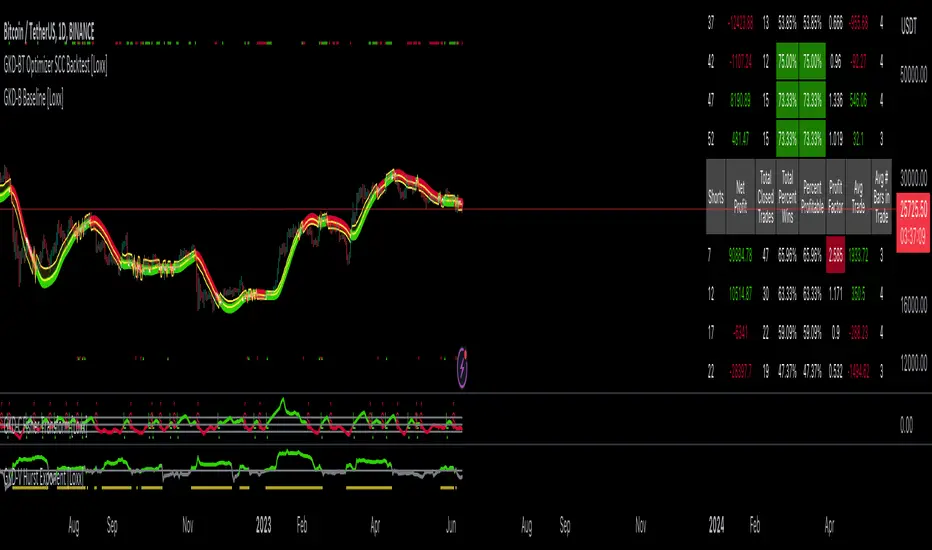
GKD-BT Optimizer SCS Backtest [Loxx]The Giga Kaleidoscope GKD-BT Optimizer SCS Backtest is a backtesting module included in Loxx's "Giga Kaleidoscope Modularized Trading System."
█ Giga Kaleidoscope GKD-BT Optimizer SCS Backtest
The Optimizer SCS Backtest is a Solo Confirmation Simple backtest that allows traders to test single GKD-C confirmation indicators across 10 varying inputs. The purpose of this backtest is to enable traders to optimize a GKD-C indicator given varying inputs.
The backtest module supports testing with 1 take profit and 1 stop loss. It also offers the option to limit testing to a specific date range, allowing simulated forward testing using historical data. This backtest module only includes standard long and short signals. Additionally, users can choose to display or hide a trading panel that provides relevant information about the backtest, statistics, and the current trade. Traders can also select a highlighting treshold for Total Percent Wins and Percent Profitable, and Profit Factor.
To use this indicator:
1. Import a GKD-C indicator "Input into NEW GKD-BT Optimizer Backtest Signals" into the GKD-C Indicator Signals dropdown
1. Import a GKD-C indicator "Input into NEW GKD-BT Optimizer Backtest Start" into the GKD-C Indicator Start dropdown
1. Import a GKD-C indicator "Input into NEW GKD-BT Optimizer Backtest Skip" into the GKD-C Indicator Skip dropdown
This backtest includes the following metrics:
1. Net profit: Overall profit or loss achieved.
2. Total Closed Trades: Total number of closed trades, both winning and losing.
3. Total Percent Wins: Total wins, whether long or short, for the selected time interval regardless of commissions and other profit-modifying addons.
4. Percent Profitable: Total wins, whether long or short, that are also profitable, taking commissions into account.
5. Profit Factor: The ratio of gross profits to gross losses, indicating how much money the strategy made for every unit of money it lost.
6. Average Profit per Trade: The average gain or loss per trade, calculated by dividing the net profit by the total number of closed trades.
7. Average Number of Bars in Trade: The average number of bars that elapsed during trades for all closed trades.
Summary of notable settings:
Input Tickers separated by commas: Allows the user to input tickers separated by commas, specifying the symbols or tickers of financial instruments used in the backtest. The tickers should follow the format "EXCHANGE:TICKER" (e.g., "NASDAQ:AAPL, NYSE:MSFT").
Import GKD-B Baseline: Imports the "GKD-B Multi-Ticker Baseline" indicator.
Import GKD-V Volatility/Volume: Imports the "GKD-V Volatility/Volume" indicator.
Import GKD-C Confirmation: Imports the "GKD-C Confirmation" indicator.
Import GKD-C Continuation: Imports the "GKD-C Continuation" indicator.
Initial Capital: Represents the starting account balance for the backtest, denominated in the base currency of the trading account.
Order Size: Determines the quantity of contracts traded in each trade.
Order Type: Specifies the type of order used in the backtest, either "Contracts" or "% Equity."
Commission: Represents the commission per order or transaction cost incurred in each trade.
**the backtest data rendered to the chart above uses $5 commission per trade and 10% equity per trade with $1 million initial capital. Each backtest result for each ticker assumes these same inputs. The results are NOT cumulative, they are separate and isolate per ticker and trading side, long or short**
█ Volatility Types included
The GKD system utilizes volatility-based take profits and stop losses. Each take profit and stop loss is calculated as a multiple of volatility. You can change the values of the multipliers in the settings as well.
This module includes 17 types of volatility:
Close-to-Close
Parkinson
Garman-Klass
Rogers-Satchell
Yang-Zhang
Garman-Klass-Yang-Zhang
Exponential Weighted Moving Average
Standard Deviation of Log Returns
Pseudo GARCH(2,2)
Average True Range
True Range Double
Standard Deviation
Adaptive Deviation
Median Absolute Deviation
Efficiency-Ratio Adaptive ATR
Mean Absolute Deviation
Static Percent
Various volatility estimators and indicators that investors and traders can use to measure the dispersion or volatility of a financial instrument's price. Each estimator has its strengths and weaknesses, and the choice of estimator should depend on the specific needs and circumstances of the user.
Close-to-Close
Close-to-Close volatility is a classic and widely used volatility measure, sometimes referred to as historical volatility.
Volatility is an indicator of the speed of a stock price change. A stock with high volatility is one where the price changes rapidly and with a larger amplitude. The more volatile a stock is, the riskier it is.
Close-to-close historical volatility is calculated using only a stock's closing prices. It is the simplest volatility estimator. However, in many cases, it is not precise enough. Stock prices could jump significantly during a trading session and return to the opening value at the end. That means that a considerable amount of price information is not taken into account by close-to-close volatility.
Despite its drawbacks, Close-to-Close volatility is still useful in cases where the instrument doesn't have intraday prices. For example, mutual funds calculate their net asset values daily or weekly, and thus their prices are not suitable for more sophisticated volatility estimators.
Parkinson
Parkinson volatility is a volatility measure that uses the stock’s high and low price of the day.
The main difference between regular volatility and Parkinson volatility is that the latter uses high and low prices for a day, rather than only the closing price. This is useful as close-to-close prices could show little difference while large price movements could have occurred during the day. Thus, Parkinson's volatility is considered more precise and requires less data for calculation than close-to-close volatility.
One drawback of this estimator is that it doesn't take into account price movements after the market closes. Hence, it systematically undervalues volatility. This drawback is addressed in the Garman-Klass volatility estimator.
Garman-Klass
Garman-Klass is a volatility estimator that incorporates open, low, high, and close prices of a security.
Garman-Klass volatility extends Parkinson's volatility by taking into account the opening and closing prices. As markets are most active during the opening and closing of a trading session, it makes volatility estimation more accurate.
Garman and Klass also assumed that the process of price change follows a continuous diffusion process (Geometric Brownian motion). However, this assumption has several drawbacks. The method is not robust for opening jumps in price and trend movements.
Despite its drawbacks, the Garman-Klass estimator is still more effective than the basic formula since it takes into account not only the price at the beginning and end of the time interval but also intraday price extremes.
Researchers Rogers and Satchell have proposed a more efficient method for assessing historical volatility that takes into account price trends. See Rogers-Satchell Volatility for more detail.
Rogers-Satchell
Rogers-Satchell is an estimator for measuring the volatility of securities with an average return not equal to zero.
Unlike Parkinson and Garman-Klass estimators, Rogers-Satchell incorporates a drift term (mean return not equal to zero). As a result, it provides better volatility estimation when the underlying is trending.
The main disadvantage of this method is that it does not take into account price movements between trading sessions. This leads to an underestimation of volatility since price jumps periodically occur in the market precisely at the moments between sessions.
A more comprehensive estimator that also considers the gaps between sessions was developed based on the Rogers-Satchel formula in the 2000s by Yang-Zhang. See Yang Zhang Volatility for more detail.
Yang-Zhang
Yang Zhang is a historical volatility estimator that handles both opening jumps and the drift and has a minimum estimation error.
Yang-Zhang volatility can be thought of as a combination of the overnight (close-to-open volatility) and a weighted average of the Rogers-Satchell volatility and the day’s open-to-close volatility. It is considered to be 14 times more efficient than the close-to-close estimator.
Garman-Klass-Yang-Zhang
Garman-Klass-Yang-Zhang (GKYZ) volatility estimator incorporates the returns of open, high, low, and closing prices in its calculation.
GKYZ volatility estimator takes into account overnight jumps but not the trend, i.e., it assumes that the underlying asset follows a Geometric Brownian Motion (GBM) process with zero drift. Therefore, the GKYZ volatility estimator tends to overestimate the volatility when the drift is different from zero. However, for a GBM process, this estimator is eight times more efficient than the close-to-close volatility estimator.
Exponential Weighted Moving Average
The Exponentially Weighted Moving Average (EWMA) is a quantitative or statistical measure used to model or describe a time series. The EWMA is widely used in finance, with the main applications being technical analysis and volatility modeling.
The moving average is designed such that older observations are given lower weights. The weights decrease exponentially as the data point gets older – hence the name exponentially weighted.
The only decision a user of the EWMA must make is the parameter lambda. The parameter decides how important the current observation is in the calculation of the EWMA. The higher the value of lambda, the more closely the EWMA tracks the original time series.
Standard Deviation of Log Returns
This is the simplest calculation of volatility. It's the standard deviation of ln(close/close(1)).
Pseudo GARCH(2,2)
This is calculated using a short- and long-run mean of variance multiplied by ?.
?avg(var;M) + (1 ? ?) avg(var;N) = 2?var/(M+1-(M-1)L) + 2(1-?)var/(M+1-(M-1)L)
Solving for ? can be done by minimizing the mean squared error of estimation; that is, regressing L^-1var - avg(var; N) against avg(var; M) - avg(var; N) and using the resulting beta estimate as ?.
Average True Range
The average true range (ATR) is a technical analysis indicator, introduced by market technician J. Welles Wilder Jr. in his book New Concepts in Technical Trading Systems, that measures market volatility by decomposing the entire range of an asset price for that period.
The true range indicator is taken as the greatest of the following: current high less the current low; the absolute value of the current high less the previous close; and the absolute value of the current low less the previous close. The ATR is then a moving average, generally using 14 days, of the true ranges.
True Range Double
A special case of ATR that attempts to correct for volatility skew.
Standard Deviation
Standard deviation is a statistic that measures the dispersion of a dataset relative to its mean and is calculated as the square root of the variance. The standard deviation is calculated as the square root of variance by determining each data point's deviation relative to the mean. If the data points are further from the mean, there is a higher deviation within the data set; thus, the more spread out the data, the higher the standard deviation.
Adaptive Deviation
By definition, the Standard Deviation (STD, also represented by the Greek letter sigma ? or the Latin letter s) is a measure that is used to quantify the amount of variation or dispersion of a set of data values. In technical analysis, we usually use it to measure the level of current volatility.
Standard Deviation is based on Simple Moving Average calculation for mean value. This version of standard deviation uses the properties of EMA to calculate what can be called a new type of deviation, and since it is based on EMA, we can call it EMA deviation. Additionally, Perry Kaufman's efficiency ratio is used to make it adaptive (since all EMA type calculations are nearly perfect for adapting).
The difference when compared to the standard is significant--not just because of EMA usage, but the efficiency ratio makes it a "bit more logical" in very volatile market conditions.
Median Absolute Deviation
The median absolute deviation is a measure of statistical dispersion. Moreover, the MAD is a robust statistic, being more resilient to outliers in a data set than the standard deviation. In the standard deviation, the distances from the mean are squared, so large deviations are weighted more heavily, and thus outliers can heavily influence it. In the MAD, the deviations of a small number of outliers are irrelevant.
Because the MAD is a more robust estimator of scale than the sample variance or standard deviation, it works better with distributions without a mean or variance, such as the Cauchy distribution.
For this indicator, a manual recreation of the quantile function in Pine Script is used. This is so users have a full inside view into how this is calculated.
Efficiency-Ratio Adaptive ATR
Average True Range (ATR) is a widely used indicator for many occasions in technical analysis. It is calculated as the RMA of the true range. This version adds a "twist": it uses Perry Kaufman's Efficiency Ratio to calculate adaptive true range.
Mean Absolute Deviation
The mean absolute deviation (MAD) is a measure of variability that indicates the average distance between observations and their mean. MAD uses the original units of the data, which simplifies interpretation. Larger values signify that the data points spread out further from the average. Conversely, lower values correspond to data points bunching closer to it. The mean absolute deviation is also known as the mean deviation and average absolute deviation.
This definition of the mean absolute deviation sounds similar to the standard deviation (SD). While both measure variability, they have different calculations. In recent years, some proponents of MAD have suggested that it replace the SD as the primary measure because it is a simpler concept that better fits real life.
█ Giga Kaleidoscope Modularized Trading System
Core components of an NNFX algorithmic trading strategy
The NNFX algorithm is built on the principles of trend, momentum, and volatility. There are six core components in the NNFX trading algorithm:
1. Volatility - price volatility; e.g., Average True Range, True Range Double, Close-to-Close, etc.
2. Baseline - a moving average to identify price trend
3. Confirmation 1 - a technical indicator used to identify trends
4. Confirmation 2 - a technical indicator used to identify trends
5. Continuation - a technical indicator used to identify trends
6. Volatility/Volume - a technical indicator used to identify volatility/volume breakouts/breakdown
7. Exit - a technical indicator used to determine when a trend is exhausted
8. Metamorphosis - a technical indicator that produces a compound signal from the combination of other GKD indicators*
*(not part of the NNFX algorithm)
What is Volatility in the NNFX trading system?
In the NNFX (No Nonsense Forex) trading system, ATR (Average True Range) is typically used to measure the volatility of an asset. It is used as a part of the system to help determine the appropriate stop loss and take profit levels for a trade. ATR is calculated by taking the average of the true range values over a specified period.
True range is calculated as the maximum of the following values:
-Current high minus the current low
-Absolute value of the current high minus the previous close
-Absolute value of the current low minus the previous close
ATR is a dynamic indicator that changes with changes in volatility. As volatility increases, the value of ATR increases, and as volatility decreases, the value of ATR decreases. By using ATR in NNFX system, traders can adjust their stop loss and take profit levels according to the volatility of the asset being traded. This helps to ensure that the trade is given enough room to move, while also minimizing potential losses.
Other types of volatility include True Range Double (TRD), Close-to-Close, and Garman-Klass
What is a Baseline indicator?
The baseline is essentially a moving average, and is used to determine the overall direction of the market.
The baseline in the NNFX system is used to filter out trades that are not in line with the long-term trend of the market. The baseline is plotted on the chart along with other indicators, such as the Moving Average (MA), the Relative Strength Index (RSI), and the Average True Range (ATR).
Trades are only taken when the price is in the same direction as the baseline. For example, if the baseline is sloping upwards, only long trades are taken, and if the baseline is sloping downwards, only short trades are taken. This approach helps to ensure that trades are in line with the overall trend of the market, and reduces the risk of entering trades that are likely to fail.
By using a baseline in the NNFX system, traders can have a clear reference point for determining the overall trend of the market, and can make more informed trading decisions. The baseline helps to filter out noise and false signals, and ensures that trades are taken in the direction of the long-term trend.
What is a Confirmation indicator?
Confirmation indicators are technical indicators that are used to confirm the signals generated by primary indicators. Primary indicators are the core indicators used in the NNFX system, such as the Average True Range (ATR), the Moving Average (MA), and the Relative Strength Index (RSI).
The purpose of the confirmation indicators is to reduce false signals and improve the accuracy of the trading system. They are designed to confirm the signals generated by the primary indicators by providing additional information about the strength and direction of the trend.
Some examples of confirmation indicators that may be used in the NNFX system include the Bollinger Bands, the MACD (Moving Average Convergence Divergence), and the MACD Oscillator. These indicators can provide information about the volatility, momentum, and trend strength of the market, and can be used to confirm the signals generated by the primary indicators.
In the NNFX system, confirmation indicators are used in combination with primary indicators and other filters to create a trading system that is robust and reliable. By using multiple indicators to confirm trading signals, the system aims to reduce the risk of false signals and improve the overall profitability of the trades.
What is a Continuation indicator?
In the NNFX (No Nonsense Forex) trading system, a continuation indicator is a technical indicator that is used to confirm a current trend and predict that the trend is likely to continue in the same direction. A continuation indicator is typically used in conjunction with other indicators in the system, such as a baseline indicator, to provide a comprehensive trading strategy.
What is a Volatility/Volume indicator?
Volume indicators, such as the On Balance Volume (OBV), the Chaikin Money Flow (CMF), or the Volume Price Trend (VPT), are used to measure the amount of buying and selling activity in a market. They are based on the trading volume of the market, and can provide information about the strength of the trend. In the NNFX system, volume indicators are used to confirm trading signals generated by the Moving Average and the Relative Strength Index. Volatility indicators include Average Direction Index, Waddah Attar, and Volatility Ratio. In the NNFX trading system, volatility is a proxy for volume and vice versa.
By using volume indicators as confirmation tools, the NNFX trading system aims to reduce the risk of false signals and improve the overall profitability of trades. These indicators can provide additional information about the market that is not captured by the primary indicators, and can help traders to make more informed trading decisions. In addition, volume indicators can be used to identify potential changes in market trends and to confirm the strength of price movements.
What is an Exit indicator?
The exit indicator is used in conjunction with other indicators in the system, such as the Moving Average (MA), the Relative Strength Index (RSI), and the Average True Range (ATR), to provide a comprehensive trading strategy.
The exit indicator in the NNFX system can be any technical indicator that is deemed effective at identifying optimal exit points. Examples of exit indicators that are commonly used include the Parabolic SAR, the Average Directional Index (ADX), and the Chandelier Exit.
The purpose of the exit indicator is to identify when a trend is likely to reverse or when the market conditions have changed, signaling the need to exit a trade. By using an exit indicator, traders can manage their risk and prevent significant losses.
In the NNFX system, the exit indicator is used in conjunction with a stop loss and a take profit order to maximize profits and minimize losses. The stop loss order is used to limit the amount of loss that can be incurred if the trade goes against the trader, while the take profit order is used to lock in profits when the trade is moving in the trader's favor.
Overall, the use of an exit indicator in the NNFX trading system is an important component of a comprehensive trading strategy. It allows traders to manage their risk effectively and improve the profitability of their trades by exiting at the right time.
What is an Metamorphosis indicator?
The concept of a metamorphosis indicator involves the integration of two or more GKD indicators to generate a compound signal. This is achieved by evaluating the accuracy of each indicator and selecting the signal from the indicator with the highest accuracy. As an illustration, let's consider a scenario where we calculate the accuracy of 10 indicators and choose the signal from the indicator that demonstrates the highest accuracy.
The resulting output from the metamorphosis indicator can then be utilized in a GKD-BT backtest by occupying a slot that aligns with the purpose of the metamorphosis indicator. The slot can be a GKD-B, GKD-C, or GKD-E slot, depending on the specific requirements and objectives of the indicator. This allows for seamless integration and utilization of the compound signal within the GKD-BT framework.
How does Loxx's GKD (Giga Kaleidoscope Modularized Trading System) implement the NNFX algorithm outlined above?
Loxx's GKD v2.0 system has five types of modules (indicators/strategies). These modules are:
1. GKD-BT - Backtesting module (Volatility, Number 1 in the NNFX algorithm)
2. GKD-B - Baseline module (Baseline and Volatility/Volume, Numbers 1 and 2 in the NNFX algorithm)
3. GKD-C - Confirmation 1/2 and Continuation module (Confirmation 1/2 and Continuation, Numbers 3, 4, and 5 in the NNFX algorithm)
4. GKD-V - Volatility/Volume module (Confirmation 1/2, Number 6 in the NNFX algorithm)
5. GKD-E - Exit module (Exit, Number 7 in the NNFX algorithm)
6. GKD-M - Metamorphosis module (Metamorphosis, Number 8 in the NNFX algorithm, but not part of the NNFX algorithm)
(additional module types will added in future releases)
Each module interacts with every module by passing data to A backtest module wherein the various components of the GKD system are combined to create a trading signal.
That is, the Baseline indicator passes its data to Volatility/Volume. The Volatility/Volume indicator passes its values to the Confirmation 1 indicator. The Confirmation 1 indicator passes its values to the Confirmation 2 indicator. The Confirmation 2 indicator passes its values to the Continuation indicator. The Continuation indicator passes its values to the Exit indicator, and finally, the Exit indicator passes its values to the Backtest strategy.
This chaining of indicators requires that each module conform to Loxx's GKD protocol, therefore allowing for the testing of every possible combination of technical indicators that make up the six components of the NNFX algorithm.
What does the application of the GKD trading system look like?
Example trading system:
Backtest: Optimizer Full GKD Backtest as shown on the chart above
Baseline: Hull Moving Average
Volatility/Volume: Hurst Exponent
Confirmation 1: Fisher Transofrm as shown on the chart above
Confirmation 2: uf2018
Continuation: Coppock Curve
Exit: Rex Oscillator
Metamorphosis: Baseline Optimizer
Each GKD indicator is denoted with a module identifier of either: GKD-BT, GKD-B, GKD-C, GKD-V, GKD-M, or GKD-E. This allows traders to understand to which module each indicator belongs and where each indicator fits into the GKD system.
█ Giga Kaleidoscope Modularized Trading System Signals
Standard Entry
1. GKD-C Confirmation gives signal
2. Baseline agrees
3. Price inside Goldie Locks Zone Minimum
4. Price inside Goldie Locks Zone Maximum
5. Confirmation 2 agrees
6. Volatility/Volume agrees
1-Candle Standard Entry
1a. GKD-C Confirmation gives signal
2a. Baseline agrees
3a. Price inside Goldie Locks Zone Minimum
4a. Price inside Goldie Locks Zone Maximum
Next Candle
1b. Price retraced
2b. Baseline agrees
3b. Confirmation 1 agrees
4b. Confirmation 2 agrees
5b. Volatility/Volume agrees
Baseline Entry
1. GKD-B Baseline gives signal
2. Confirmation 1 agrees
3. Price inside Goldie Locks Zone Minimum
4. Price inside Goldie Locks Zone Maximum
5. Confirmation 2 agrees
6. Volatility/Volume agrees
7. Confirmation 1 signal was less than 'Maximum Allowable PSBC Bars Back' prior
1-Candle Baseline Entry
1a. GKD-B Baseline gives signal
2a. Confirmation 1 agrees
3a. Price inside Goldie Locks Zone Minimum
4a. Price inside Goldie Locks Zone Maximum
5a. Confirmation 1 signal was less than 'Maximum Allowable PSBC Bars Back' prior
Next Candle
1b. Price retraced
2b. Baseline agrees
3b. Confirmation 1 agrees
4b. Confirmation 2 agrees
5b. Volatility/Volume agrees
Volatility/Volume Entry
1. GKD-V Volatility/Volume gives signal
2. Confirmation 1 agrees
3. Price inside Goldie Locks Zone Minimum
4. Price inside Goldie Locks Zone Maximum
5. Confirmation 2 agrees
6. Baseline agrees
7. Confirmation 1 signal was less than 7 candles prior
1-Candle Volatility/Volume Entry
1a. GKD-V Volatility/Volume gives signal
2a. Confirmation 1 agrees
3a. Price inside Goldie Locks Zone Minimum
4a. Price inside Goldie Locks Zone Maximum
5a. Confirmation 1 signal was less than 'Maximum Allowable PSVVC Bars Back' prior
Next Candle
1b. Price retraced
2b. Volatility/Volume agrees
3b. Confirmation 1 agrees
4b. Confirmation 2 agrees
5b. Baseline agrees
Confirmation 2 Entry
1. GKD-C Confirmation 2 gives signal
2. Confirmation 1 agrees
3. Price inside Goldie Locks Zone Minimum
4. Price inside Goldie Locks Zone Maximum
5. Volatility/Volume agrees
6. Baseline agrees
7. Confirmation 1 signal was less than 7 candles prior
1-Candle Confirmation 2 Entry
1a. GKD-C Confirmation 2 gives signal
2a. Confirmation 1 agrees
3a. Price inside Goldie Locks Zone Minimum
4a. Price inside Goldie Locks Zone Maximum
5a. Confirmation 1 signal was less than 'Maximum Allowable PSC2C Bars Back' prior
Next Candle
1b. Price retraced
2b. Confirmation 2 agrees
3b. Confirmation 1 agrees
4b. Volatility/Volume agrees
5b. Baseline agrees
PullBack Entry
1a. GKD-B Baseline gives signal
2a. Confirmation 1 agrees
3a. Price is beyond 1.0x Volatility of Baseline
Next Candle
1b. Price inside Goldie Locks Zone Minimum
2b. Price inside Goldie Locks Zone Maximum
3b. Confirmation 1 agrees
4b. Confirmation 2 agrees
5b. Volatility/Volume agrees
Continuation Entry
1. Standard Entry, 1-Candle Standard Entry, Baseline Entry, 1-Candle Baseline Entry, Volatility/Volume Entry, 1-Candle Volatility/Volume Entry, Confirmation 2 Entry, 1-Candle Confirmation 2 Entry, or Pullback entry triggered previously
2. Baseline hasn't crossed since entry signal trigger
4. Confirmation 1 agrees
5. Baseline agrees
6. Confirmation 2 agrees
█ Connecting to Backtests
All GKD indicators are chained indicators meaning you export the value of the indicators to specialized backtest to creat your GKD trading system. Each indicator contains a proprietary signal generation algo that will only work with GKD backtests. You can find these backtests using the links below.
GKD-BT Giga Confirmation Stack Backtest
GKD-BT Giga Stacks Backtest
GKD-BT Full Giga Kaleidoscope Backtest
GKD-BT Solo Confirmation Super Complex Backtest
GKD-BT Solo Confirmation Complex Backtest
GKD-BT Solo Confirmation Simple Backtest
GKD-M Baseline Optimizer
GKD-M Accuracy Alchemist
GKD-BT Optimizer SCC Backtest
GKD-BT Optimizer SCS Backtest
GKD-BT Optimizer SCS Backtest
GKD-C GKD-BT Optimizer Full GKD Backtest
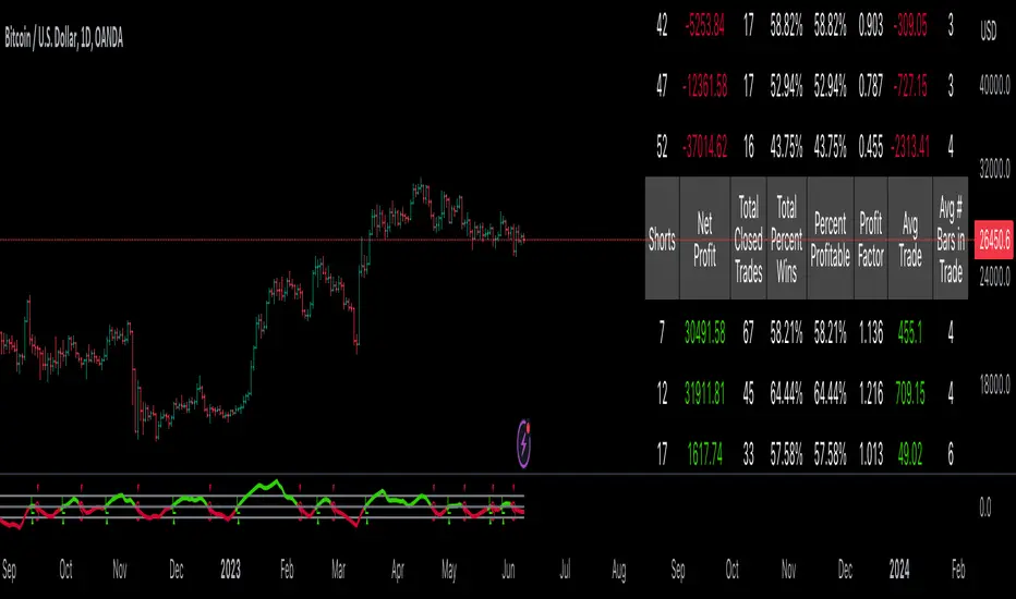
GKD-BT Multi-Ticker Full GKD Backtest [Loxx]The Giga Kaleidoscope GKD-BT Multi-Ticker Full GKD Backtest is a backtesting module included in Loxx's "Giga Kaleidoscope Modularized Trading System."
█ Giga Kaleidoscope GKD-BT Multi-Ticker Full GKD Backtest
The Multi-Ticker Full GKD Backtest is a Full GKD backtest that allows traders to test single GKD-C Confirmation indicator filtered by a GKD-B Multi-Ticker Baseline, GKD-V Volatility/Volume, and GKD-C Confirmation 2 indicator across 1-10 tickers. In addition. this module adds on various other long and short signls that fall outside the normal GKD standard long and short signals. These additional signals are formed using the GKD-B Multi-Ticker Baseline, GKD-V Volatility/Volume, GKD-C Confirmation 2, and GKD-C Continuation indicators. The purpose of this backtest is to enable traders to quickly evaluate a Baseline, Volatility/Volume, Confirmation 2, and Continuation indicators filtered GKD-C Confirmation 1 indicator across hundreds of tickers within 30-60 minutes.
The backtest module supports testing with 1 take profit and 1 stop loss. It also offers the option to limit testing to a specific date range, allowing simulated forward testing using historical data. This backtest module only includes standard long and short signals. Additionally, users can choose to display or hide a trading panel that provides relevant information about the backtest, statistics, and the current trade. Traders can also select a highlighting threshold for Total Percent Wins and Percent Profitable, and Profit Factor.
To use this indicator:
1. Import 1-10 tickers into the GKD-B Multi-Ticker Baseline indicator
2. Import the value "Input into NEW GKD-BT Multi-ticker Backtest" from the GKD-B Multi-Ticker Baseline indicator into the GKD-BT Multi-Ticker Full GKD Backtest.
3. Select the "Multi-ticker" option in the GKD-V Volatility/Volume indicator
4. Import 1-10 tickers into the GKD-V Volatility/Volume indicator
5. Import the value "Input into NEW GKD-BT Multi-ticker Backtest" from the GKD-V Volatility/Volume indicator into the GKD-BT Multi-Ticker Full GKD Backtest.
6. Select the "Multi-ticker" option in the GKD-C Confirmation 1 indicator.
7. Import 1-10 tickers into the GKD-C Confirmation 1 indicator.
8. Import the same 1-10 indicators into the GKD-BT Multi-Ticker Full GKD Backtest.
9. Import the value "Input into NEW GKD-BT Multi-ticker Backtest" from the GKD-C Confirmation 1 indicator into the GKD-BT Multi-Ticker Full GKD Backtest.
10. Import 1-10 tickers into the GKD-C Confirmation 2 indicator.
11. Import the same 1-10 indicators into the GKD-BT Multi-Ticker Full GKD Backtest.
12. Import the value "Input into NEW GKD-BT Multi-ticker Backtest" from the GKD-C Confirmation 2 indicator into the GKD-BT Multi-Ticker Full GKD Backtest.
13. Import 1-10 tickers into the GKD-C Continuation indicator.
14. Import the same 1-10 indicators into the GKD-BT Multi-Ticker Full GKD Backtest.
15. Import the value "Input into NEW GKD-BT Multi-ticker Backtest" from the GKD-C Continuation indicator into the GKD-BT Multi-Ticker Full GKD Backtest.
16. When importing tickers, ensure that you import the same type of tickers for all 1-10 tickers. For example, test only FX or Cryptocurrency or Stocks. Do not combine different tradable asset types.
17. Make sure that your chart is set to a ticker that corresponds to the tradable asset type. For cryptocurrency testing, set the chart to BTCUSDT. For Forex testing, set the chart to EURUSD.
This backtest includes the following metrics:
1. Net profit: Overall profit or loss achieved.
2. Total Closed Trades: Total number of closed trades, both winning and losing.
3. Total Percent Wins: Total wins, whether long or short, for the selected time interval regardless of commissions and other profit-modifying addons.
4. Percent Profitable: Total wins, whether long or short, that are also profitable, taking commissions into account.
5. Profit Factor: The ratio of gross profits to gross losses, indicating how much money the strategy made for every unit of money it lost.
6. Average Profit per Trade: The average gain or loss per trade, calculated by dividing the net profit by the total number of closed trades.
7. Average Number of Bars in Trade: The average number of bars that elapsed during trades for all closed trades.
Summary of notable settings:
Input Tickers separated by commas: Allows the user to input tickers separated by commas, specifying the symbols or tickers of financial instruments used in the backtest. The tickers should follow the format "EXCHANGE:TICKER" (e.g., "NASDAQ:AAPL, NYSE:MSFT").
Import GKD-B Baseline: Imports the "GKD-B Multi-Ticker Baseline" indicator.
Import GKD-V Volatility/Volume: Imports the "GKD-V Volatility/Volume" indicator.
Import GKD-C Confirmation: Imports the "GKD-C" indicator.
Activate Baseline: Activates the GKD-B Multi-Ticker Baseline.
Activate Goldie Locks Zone Minimum Threshold: Activates the inner Goldie Locks Zone from the GKD-B Multi-Ticker Baseline
Activate Goldie Locks Zone Maximum Threshold: Activates the outer Goldie Locks Zone from the GKD-B Multi-Ticker Baseline
Activate Volatility/Volume: Activates the GKD-V Volatility/Volume indicator.
Initial Capital: Represents the starting account balance for the backtest, denominated in the base currency of the trading account.
Order Size: Determines the quantity of contracts traded in each trade.
Order Type: Specifies the type of order used in the backtest, either "Contracts" or "% Equity."
Commission: Represents the commission per order or transaction cost incurred in each trade.
**the backtest data rendered to the chart above uses $5 commission per trade and 10% equity per trade with $1 million initial capital. Each backtest result for each ticker assumes these same inputs. The results are NOT cumulative, they are separate and isolate per ticker and trading side, long or short**
█ Volatility Types included
The GKD system utilizes volatility-based take profits and stop losses. Each take profit and stop loss is calculated as a multiple of volatility. You can change the values of the multipliers in the settings as well.
This module includes 17 types of volatility:
Close-to-Close
Parkinson
Garman-Klass
Rogers-Satchell
Yang-Zhang
Garman-Klass-Yang-Zhang
Exponential Weighted Moving Average
Standard Deviation of Log Returns
Pseudo GARCH(2,2)
Average True Range
True Range Double
Standard Deviation
Adaptive Deviation
Median Absolute Deviation
Efficiency-Ratio Adaptive ATR
Mean Absolute Deviation
Static Percent
Various volatility estimators and indicators that investors and traders can use to measure the dispersion or volatility of a financial instrument's price. Each estimator has its strengths and weaknesses, and the choice of estimator should depend on the specific needs and circumstances of the user.
Close-to-Close
Close-to-Close volatility is a classic and widely used volatility measure, sometimes referred to as historical volatility.
Volatility is an indicator of the speed of a stock price change. A stock with high volatility is one where the price changes rapidly and with a larger amplitude. The more volatile a stock is, the riskier it is.
Close-to-close historical volatility is calculated using only a stock's closing prices. It is the simplest volatility estimator. However, in many cases, it is not precise enough. Stock prices could jump significantly during a trading session and return to the opening value at the end. That means that a considerable amount of price information is not taken into account by close-to-close volatility.
Despite its drawbacks, Close-to-Close volatility is still useful in cases where the instrument doesn't have intraday prices. For example, mutual funds calculate their net asset values daily or weekly, and thus their prices are not suitable for more sophisticated volatility estimators.
Parkinson
Parkinson volatility is a volatility measure that uses the stock’s high and low price of the day.
The main difference between regular volatility and Parkinson volatility is that the latter uses high and low prices for a day, rather than only the closing price. This is useful as close-to-close prices could show little difference while large price movements could have occurred during the day. Thus, Parkinson's volatility is considered more precise and requires less data for calculation than close-to-close volatility.
One drawback of this estimator is that it doesn't take into account price movements after the market closes. Hence, it systematically undervalues volatility. This drawback is addressed in the Garman-Klass volatility estimator.
Garman-Klass
Garman-Klass is a volatility estimator that incorporates open, low, high, and close prices of a security.
Garman-Klass volatility extends Parkinson's volatility by taking into account the opening and closing prices. As markets are most active during the opening and closing of a trading session, it makes volatility estimation more accurate.
Garman and Klass also assumed that the process of price change follows a continuous diffusion process (Geometric Brownian motion). However, this assumption has several drawbacks. The method is not robust for opening jumps in price and trend movements.
Despite its drawbacks, the Garman-Klass estimator is still more effective than the basic formula since it takes into account not only the price at the beginning and end of the time interval but also intraday price extremes.
Researchers Rogers and Satchell have proposed a more efficient method for assessing historical volatility that takes into account price trends. See Rogers-Satchell Volatility for more detail.
Rogers-Satchell
Rogers-Satchell is an estimator for measuring the volatility of securities with an average return not equal to zero.
Unlike Parkinson and Garman-Klass estimators, Rogers-Satchell incorporates a drift term (mean return not equal to zero). As a result, it provides better volatility estimation when the underlying is trending.
The main disadvantage of this method is that it does not take into account price movements between trading sessions. This leads to an underestimation of volatility since price jumps periodically occur in the market precisely at the moments between sessions.
A more comprehensive estimator that also considers the gaps between sessions was developed based on the Rogers-Satchel formula in the 2000s by Yang-Zhang. See Yang Zhang Volatility for more detail.
Yang-Zhang
Yang Zhang is a historical volatility estimator that handles both opening jumps and the drift and has a minimum estimation error.
Yang-Zhang volatility can be thought of as a combination of the overnight (close-to-open volatility) and a weighted average of the Rogers-Satchell volatility and the day’s open-to-close volatility. It is considered to be 14 times more efficient than the close-to-close estimator.
Garman-Klass-Yang-Zhang
Garman-Klass-Yang-Zhang (GKYZ) volatility estimator incorporates the returns of open, high, low, and closing prices in its calculation.
GKYZ volatility estimator takes into account overnight jumps but not the trend, i.e., it assumes that the underlying asset follows a Geometric Brownian Motion (GBM) process with zero drift. Therefore, the GKYZ volatility estimator tends to overestimate the volatility when the drift is different from zero. However, for a GBM process, this estimator is eight times more efficient than the close-to-close volatility estimator.
Exponential Weighted Moving Average
The Exponentially Weighted Moving Average (EWMA) is a quantitative or statistical measure used to model or describe a time series. The EWMA is widely used in finance, with the main applications being technical analysis and volatility modeling.
The moving average is designed such that older observations are given lower weights. The weights decrease exponentially as the data point gets older – hence the name exponentially weighted.
The only decision a user of the EWMA must make is the parameter lambda. The parameter decides how important the current observation is in the calculation of the EWMA. The higher the value of lambda, the more closely the EWMA tracks the original time series.
Standard Deviation of Log Returns
This is the simplest calculation of volatility. It's the standard deviation of ln(close/close(1)).
Pseudo GARCH(2,2)
This is calculated using a short- and long-run mean of variance multiplied by ?.
?avg(var;M) + (1 ? ?) avg(var;N) = 2?var/(M+1-(M-1)L) + 2(1-?)var/(M+1-(M-1)L)
Solving for ? can be done by minimizing the mean squared error of estimation; that is, regressing L^-1var - avg(var; N) against avg(var; M) - avg(var; N) and using the resulting beta estimate as ?.
Average True Range
The average true range (ATR) is a technical analysis indicator, introduced by market technician J. Welles Wilder Jr. in his book New Concepts in Technical Trading Systems, that measures market volatility by decomposing the entire range of an asset price for that period.
The true range indicator is taken as the greatest of the following: current high less the current low; the absolute value of the current high less the previous close; and the absolute value of the current low less the previous close. The ATR is then a moving average, generally using 14 days, of the true ranges.
True Range Double
A special case of ATR that attempts to correct for volatility skew.
Standard Deviation
Standard deviation is a statistic that measures the dispersion of a dataset relative to its mean and is calculated as the square root of the variance. The standard deviation is calculated as the square root of variance by determining each data point's deviation relative to the mean. If the data points are further from the mean, there is a higher deviation within the data set; thus, the more spread out the data, the higher the standard deviation.
Adaptive Deviation
By definition, the Standard Deviation (STD, also represented by the Greek letter sigma ? or the Latin letter s) is a measure that is used to quantify the amount of variation or dispersion of a set of data values. In technical analysis, we usually use it to measure the level of current volatility.
Standard Deviation is based on Simple Moving Average calculation for mean value. This version of standard deviation uses the properties of EMA to calculate what can be called a new type of deviation, and since it is based on EMA, we can call it EMA deviation. Additionally, Perry Kaufman's efficiency ratio is used to make it adaptive (since all EMA type calculations are nearly perfect for adapting).
The difference when compared to the standard is significant--not just because of EMA usage, but the efficiency ratio makes it a "bit more logical" in very volatile market conditions.
Median Absolute Deviation
The median absolute deviation is a measure of statistical dispersion. Moreover, the MAD is a robust statistic, being more resilient to outliers in a data set than the standard deviation. In the standard deviation, the distances from the mean are squared, so large deviations are weighted more heavily, and thus outliers can heavily influence it. In the MAD, the deviations of a small number of outliers are irrelevant.
Because the MAD is a more robust estimator of scale than the sample variance or standard deviation, it works better with distributions without a mean or variance, such as the Cauchy distribution.
For this indicator, a manual recreation of the quantile function in Pine Script is used. This is so users have a full inside view into how this is calculated.
Efficiency-Ratio Adaptive ATR
Average True Range (ATR) is a widely used indicator for many occasions in technical analysis. It is calculated as the RMA of the true range. This version adds a "twist": it uses Perry Kaufman's Efficiency Ratio to calculate adaptive true range.
Mean Absolute Deviation
The mean absolute deviation (MAD) is a measure of variability that indicates the average distance between observations and their mean. MAD uses the original units of the data, which simplifies interpretation. Larger values signify that the data points spread out further from the average. Conversely, lower values correspond to data points bunching closer to it. The mean absolute deviation is also known as the mean deviation and average absolute deviation.
This definition of the mean absolute deviation sounds similar to the standard deviation (SD). While both measure variability, they have different calculations. In recent years, some proponents of MAD have suggested that it replace the SD as the primary measure because it is a simpler concept that better fits real life.
█ Giga Kaleidoscope Modularized Trading System
Core components of an NNFX algorithmic trading strategy
The NNFX algorithm is built on the principles of trend, momentum, and volatility. There are six core components in the NNFX trading algorithm:
1. Volatility - price volatility; e.g., Average True Range, True Range Double, Close-to-Close, etc.
2. Baseline - a moving average to identify price trend
3. Confirmation 1 - a technical indicator used to identify trends
4. Confirmation 2 - a technical indicator used to identify trends
5. Continuation - a technical indicator used to identify trends
6. Volatility/Volume - a technical indicator used to identify volatility/volume breakouts/breakdown
7. Exit - a technical indicator used to determine when a trend is exhausted
8. Metamorphosis - a technical indicator that produces a compound signal from the combination of other GKD indicators*
*(not part of the NNFX algorithm)
What is Volatility in the NNFX trading system?
In the NNFX (No Nonsense Forex) trading system, ATR (Average True Range) is typically used to measure the volatility of an asset. It is used as a part of the system to help determine the appropriate stop loss and take profit levels for a trade. ATR is calculated by taking the average of the true range values over a specified period.
True range is calculated as the maximum of the following values:
-Current high minus the current low
-Absolute value of the current high minus the previous close
-Absolute value of the current low minus the previous close
ATR is a dynamic indicator that changes with changes in volatility. As volatility increases, the value of ATR increases, and as volatility decreases, the value of ATR decreases. By using ATR in NNFX system, traders can adjust their stop loss and take profit levels according to the volatility of the asset being traded. This helps to ensure that the trade is given enough room to move, while also minimizing potential losses.
Other types of volatility include True Range Double (TRD), Close-to-Close, and Garman-Klass
What is a Baseline indicator?
The baseline is essentially a moving average, and is used to determine the overall direction of the market.
The baseline in the NNFX system is used to filter out trades that are not in line with the long-term trend of the market. The baseline is plotted on the chart along with other indicators, such as the Moving Average (MA), the Relative Strength Index (RSI), and the Average True Range (ATR).
Trades are only taken when the price is in the same direction as the baseline. For example, if the baseline is sloping upwards, only long trades are taken, and if the baseline is sloping downwards, only short trades are taken. This approach helps to ensure that trades are in line with the overall trend of the market, and reduces the risk of entering trades that are likely to fail.
By using a baseline in the NNFX system, traders can have a clear reference point for determining the overall trend of the market, and can make more informed trading decisions. The baseline helps to filter out noise and false signals, and ensures that trades are taken in the direction of the long-term trend.
What is a Confirmation indicator?
Confirmation indicators are technical indicators that are used to confirm the signals generated by primary indicators. Primary indicators are the core indicators used in the NNFX system, such as the Average True Range (ATR), the Moving Average (MA), and the Relative Strength Index (RSI).
The purpose of the confirmation indicators is to reduce false signals and improve the accuracy of the trading system. They are designed to confirm the signals generated by the primary indicators by providing additional information about the strength and direction of the trend.
Some examples of confirmation indicators that may be used in the NNFX system include the Bollinger Bands, the MACD (Moving Average Convergence Divergence), and the MACD Oscillator. These indicators can provide information about the volatility, momentum, and trend strength of the market, and can be used to confirm the signals generated by the primary indicators.
In the NNFX system, confirmation indicators are used in combination with primary indicators and other filters to create a trading system that is robust and reliable. By using multiple indicators to confirm trading signals, the system aims to reduce the risk of false signals and improve the overall profitability of the trades.
What is a Continuation indicator?
In the NNFX (No Nonsense Forex) trading system, a continuation indicator is a technical indicator that is used to confirm a current trend and predict that the trend is likely to continue in the same direction. A continuation indicator is typically used in conjunction with other indicators in the system, such as a baseline indicator, to provide a comprehensive trading strategy.
What is a Volatility/Volume indicator?
Volume indicators, such as the On Balance Volume (OBV), the Chaikin Money Flow (CMF), or the Volume Price Trend (VPT), are used to measure the amount of buying and selling activity in a market. They are based on the trading volume of the market, and can provide information about the strength of the trend. In the NNFX system, volume indicators are used to confirm trading signals generated by the Moving Average and the Relative Strength Index. Volatility indicators include Average Direction Index, Waddah Attar, and Volatility Ratio. In the NNFX trading system, volatility is a proxy for volume and vice versa.
By using volume indicators as confirmation tools, the NNFX trading system aims to reduce the risk of false signals and improve the overall profitability of trades. These indicators can provide additional information about the market that is not captured by the primary indicators, and can help traders to make more informed trading decisions. In addition, volume indicators can be used to identify potential changes in market trends and to confirm the strength of price movements.
What is an Exit indicator?
The exit indicator is used in conjunction with other indicators in the system, such as the Moving Average (MA), the Relative Strength Index (RSI), and the Average True Range (ATR), to provide a comprehensive trading strategy.
The exit indicator in the NNFX system can be any technical indicator that is deemed effective at identifying optimal exit points. Examples of exit indicators that are commonly used include the Parabolic SAR, the Average Directional Index (ADX), and the Chandelier Exit.
The purpose of the exit indicator is to identify when a trend is likely to reverse or when the market conditions have changed, signaling the need to exit a trade. By using an exit indicator, traders can manage their risk and prevent significant losses.
In the NNFX system, the exit indicator is used in conjunction with a stop loss and a take profit order to maximize profits and minimize losses. The stop loss order is used to limit the amount of loss that can be incurred if the trade goes against the trader, while the take profit order is used to lock in profits when the trade is moving in the trader's favor.
Overall, the use of an exit indicator in the NNFX trading system is an important component of a comprehensive trading strategy. It allows traders to manage their risk effectively and improve the profitability of their trades by exiting at the right time.
What is an Metamorphosis indicator?
The concept of a metamorphosis indicator involves the integration of two or more GKD indicators to generate a compound signal. This is achieved by evaluating the accuracy of each indicator and selecting the signal from the indicator with the highest accuracy. As an illustration, let's consider a scenario where we calculate the accuracy of 10 indicators and choose the signal from the indicator that demonstrates the highest accuracy.
The resulting output from the metamorphosis indicator can then be utilized in a GKD-BT backtest by occupying a slot that aligns with the purpose of the metamorphosis indicator. The slot can be a GKD-B, GKD-C, or GKD-E slot, depending on the specific requirements and objectives of the indicator. This allows for seamless integration and utilization of the compound signal within the GKD-BT framework.
How does Loxx's GKD (Giga Kaleidoscope Modularized Trading System) implement the NNFX algorithm outlined above?
Loxx's GKD v2.0 system has five types of modules (indicators/strategies). These modules are:
1. GKD-BT - Backtesting module (Volatility, Number 1 in the NNFX algorithm)
2. GKD-B - Baseline module (Baseline and Volatility/Volume, Numbers 1 and 2 in the NNFX algorithm)
3. GKD-C - Confirmation 1/2 and Continuation module (Confirmation 1/2 and Continuation, Numbers 3, 4, and 5 in the NNFX algorithm)
4. GKD-V - Volatility/Volume module (Confirmation 1/2, Number 6 in the NNFX algorithm)
5. GKD-E - Exit module (Exit, Number 7 in the NNFX algorithm)
6. GKD-M - Metamorphosis module (Metamorphosis, Number 8 in the NNFX algorithm, but not part of the NNFX algorithm)
(additional module types will added in future releases)
Each module interacts with every module by passing data to A backtest module wherein the various components of the GKD system are combined to create a trading signal.
That is, the Baseline indicator passes its data to Volatility/Volume. The Volatility/Volume indicator passes its values to the Confirmation 1 indicator. The Confirmation 1 indicator passes its values to the Confirmation 2 indicator. The Confirmation 2 indicator passes its values to the Continuation indicator. The Continuation indicator passes its values to the Exit indicator, and finally, the Exit indicator passes its values to the Backtest strategy.
This chaining of indicators requires that each module conform to Loxx's GKD protocol, therefore allowing for the testing of every possible combination of technical indicators that make up the six components of the NNFX algorithm.
What does the application of the GKD trading system look like?
Example trading system:
Backtest: Multi-Ticker Full GKD Backtest as shown on the chart above
Baseline: Hull Moving Average as shown on the chart above
Volatility/Volume: Hurst Exponent as shown on the chart above
Confirmation 1: Fisher Transform as shown on the chart above
Confirmation 2: uf2018 as shown on the chart above
Continuation: Coppock Curve as shown on the chart above
Exit: Rex Oscillator
Metamorphosis: Baseline Optimizer
Each GKD indicator is denoted with a module identifier of either: GKD-BT, GKD-B, GKD-C, GKD-V, GKD-M, or GKD-E. This allows traders to understand to which module each indicator belongs and where each indicator fits into the GKD system.
█ Giga Kaleidoscope Modularized Trading System Signals
Standard Entry
1. GKD-C Confirmation gives signal
2. Baseline agrees
3. Price inside Goldie Locks Zone Minimum
4. Price inside Goldie Locks Zone Maximum
5. Confirmation 2 agrees
6. Volatility/Volume agrees
1-Candle Standard Entry
1a. GKD-C Confirmation gives signal
2a. Baseline agrees
3a. Price inside Goldie Locks Zone Minimum
4a. Price inside Goldie Locks Zone Maximum
Next Candle
1b. Price retraced
2b. Baseline agrees
3b. Confirmation 1 agrees
4b. Confirmation 2 agrees
5b. Volatility/Volume agrees
Baseline Entry
1. GKD-B Basline gives signal
2. Confirmation 1 agrees
3. Price inside Goldie Locks Zone Minimum
4. Price inside Goldie Locks Zone Maximum
5. Confirmation 2 agrees
6. Volatility/Volume agrees
7. Confirmation 1 signal was less than 'Maximum Allowable PSBC Bars Back' prior
1-Candle Baseline Entry
1a. GKD-B Baseline gives signal
2a. Confirmation 1 agrees
3a. Price inside Goldie Locks Zone Minimum
4a. Price inside Goldie Locks Zone Maximum
5a. Confirmation 1 signal was less than 'Maximum Allowable PSBC Bars Back' prior
Next Candle
1b. Price retraced
2b. Baseline agrees
3b. Confirmation 1 agrees
4b. Confirmation 2 agrees
5b. Volatility/Volume agrees
Volatility/Volume Entry
1. GKD-V Volatility/Volume gives signal
2. Confirmation 1 agrees
3. Price inside Goldie Locks Zone Minimum
4. Price inside Goldie Locks Zone Maximum
5. Confirmation 2 agrees
6. Baseline agrees
7. Confirmation 1 signal was less than 7 candles prior
1-Candle Volatility/Volume Entry
1a. GKD-V Volatility/Volume gives signal
2a. Confirmation 1 agrees
3a. Price inside Goldie Locks Zone Minimum
4a. Price inside Goldie Locks Zone Maximum
5a. Confirmation 1 signal was less than 'Maximum Allowable PSVVC Bars Back' prior
Next Candle
1b. Price retraced
2b. Volatility/Volume agrees
3b. Confirmation 1 agrees
4b. Confirmation 2 agrees
5b. Baseline agrees
Confirmation 2 Entry
1. GKD-C Confirmation 2 gives signal
2. Confirmation 1 agrees
3. Price inside Goldie Locks Zone Minimum
4. Price inside Goldie Locks Zone Maximum
5. Volatility/Volume agrees
6. Baseline agrees
7. Confirmation 1 signal was less than 7 candles prior
1-Candle Confirmation 2 Entry
1a. GKD-C Confirmation 2 gives signal
2a. Confirmation 1 agrees
3a. Price inside Goldie Locks Zone Minimum
4a. Price inside Goldie Locks Zone Maximum
5a. Confirmation 1 signal was less than 'Maximum Allowable PSC2C Bars Back' prior
Next Candle
1b. Price retraced
2b. Confirmation 2 agrees
3b. Confirmation 1 agrees
4b. Volatility/Volume agrees
5b. Baseline agrees
PullBack Entry
1a. GKD-B Baseline gives signal
2a. Confirmation 1 agrees
3a. Price is beyond 1.0x Volatility of Baseline
Next Candle
1b. Price inside Goldie Locks Zone Minimum
2b. Price inside Goldie Locks Zone Maximum
3b. Confirmation 1 agrees
4b. Confirmation 2 agrees
5b. Volatility/Volume agrees
Continuation Entry
1. Standard Entry, 1-Candle Standard Entry, Baseline Entry, 1-Candle Baseline Entry, Volatility/Volume Entry, 1-Candle Volatility/Volume Entry, Confirmation 2 Entry, 1-Candle Confirmation 2 Entry, or Pullback entry triggered previously
2. Baseline hasn't crossed since entry signal trigger
4. Confirmation 1 agrees
5. Baseline agrees
6. Confirmation 2 agrees
█ Connecting to Backtests
All GKD indicators are chained indicators meaning you export the value of the indicators to specialized backtest to creat your GKD trading system. Each indicator contains a proprietary signal generation algo that will only work with GKD backtests. You can find these backtests using the links below.
GKD-BT Giga Confirmation Stack Backtest
GKD-BT Giga Stacks Backtest
GKD-BT Full Giga Kaleidoscope Backtest
GKD-BT Solo Confirmation Super Complex Backtest
GKD-BT Solo Confirmation Complex Backtest
GKD-BT Solo Confirmation Simple Backtest
GKD-M Baseline Optimizer
GKD-M Accuracy Alchemist
GKD-BT Multi-Ticker SCC Backtest
GKD-BT Multi-Ticker SCS Backtest
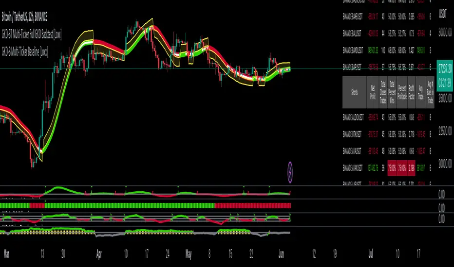
GKD-BT Multi-Ticker SCSC Backtest [Loxx]The Giga Kaleidoscope GKD-BT Multi-Ticker SCSC Backtest is a backtesting module included in Loxx's "Giga Kaleidoscope Modularized Trading System."
█ Giga Kaleidoscope GKD-BT Multi-Ticker SCSC Backtest
The Multi-Ticker SCSC Backtest is a Solo Confirmation Super Complex backtest that allows traders to test single GKD-C Confirmation indicator filtered by both a GKD-B Multi-Ticker Baseline and GKD-V Volatility/Volume indicator across 1-10 tickers. In addition. this module adds on various other long and short signls that fall outside the normal GKD standard long and short signals. These additional signals are formed using the GKD-B Multi-Ticker Baseline, GKD-V Volatility/Volume, and GKD-C Continuation indicators. The purpose of this backtest is to enable traders to quickly evaluate a Baseline, Volatility/Volume, and Continuation indicators filtered GKD-C Confirmation 1 indicator across hundreds of tickers within 30-60 minutes.
The backtest module supports testing with 1 take profit and 1 stop loss. It also offers the option to limit testing to a specific date range, allowing simulated forward testing using historical data. This backtest module only includes standard long and short signals. Additionally, users can choose to display or hide a trading panel that provides relevant information about the backtest, statistics, and the current trade. Traders can also select a highlighting threshold for Total Percent Wins and Percent Profitable, and Profit Factor.
To use this indicator:
1. Import 1-10 tickers into the GKD-B Multi-Ticker Baseline indicator
2. Import the value "Input into NEW GKD-BT Multi-ticker Backtest" from the GKD-B Multi-Ticker Baseline indicator into the GKD-BT Multi-Ticker SCSC Backtest.
3. Select the "Multi-ticker" option in the GKD-V Volatility/Volume indicator
4. Import 1-10 tickers into the GKD-V Volatility/Volume indicator
5. Import the value "Input into NEW GKD-BT Multi-ticker Backtest" from the GKD-V Volatility/Volume indicator into the GKD-BT Multi-Ticker SCSC Backtest.
6. Select the "Multi-ticker" option in the GKD-C Confirmation indicator.
7. Import 1-10 tickers into the GKD-C Confirmation indicator.
8. Import the same 1-10 indicators into the GKD-BT Multi-Ticker SCSC Backtest.
9. Import the value "Input into NEW GKD-BT Multi-ticker Backtest" from the GKD-C Confirmation indicator into the GKD-BT Multi-Ticker SCSC Backtest.
10. Import 1-10 tickers into the GKD-C Continuation indicator.
11. Import the same 1-10 indicators into the GKD-BT Multi-Ticker SCSC Backtest.
12. Import the value "Input into NEW GKD-BT Multi-ticker Backtest" from the GKD-C Continuation indicator into the GKD-BT Multi-Ticker SCSC Backtest.
13. When importing tickers, ensure that you import the same type of tickers for all 1-10 tickers. For example, test only FX or Cryptocurrency or Stocks. Do not combine different tradable asset types.
14. Make sure that your chart is set to a ticker that corresponds to the tradable asset type. For cryptocurrency testing, set the chart to BTCUSDT. For Forex testing, set the chart to EURUSD.
This backtest includes the following metrics:
1. Net profit: Overall profit or loss achieved.
2. Total Closed Trades: Total number of closed trades, both winning and losing.
3. Total Percent Wins: Total wins, whether long or short, for the selected time interval regardless of commissions and other profit-modifying addons.
4. Percent Profitable: Total wins, whether long or short, that are also profitable, taking commissions into account.
5. Profit Factor: The ratio of gross profits to gross losses, indicating how much money the strategy made for every unit of money it lost.
6. Average Profit per Trade: The average gain or loss per trade, calculated by dividing the net profit by the total number of closed trades.
7. Average Number of Bars in Trade: The average number of bars that elapsed during trades for all closed trades.
Summary of notable settings:
Input Tickers separated by commas: Allows the user to input tickers separated by commas, specifying the symbols or tickers of financial instruments used in the backtest. The tickers should follow the format "EXCHANGE:TICKER" (e.g., "NASDAQ:AAPL, NYSE:MSFT").
Import GKD-B Baseline: Imports the "GKD-B Multi-Ticker Baseline" indicator.
Import GKD-V Volatility/Volume: Imports the "GKD-V Volatility/Volume" indicator.
Import GKD-C Confirmation: Imports the "GKD-C Confirmation" indicator.
Import GKD-C Continuation: Imports the "GKD-C Continuation" indicator.
Initial Capital: Represents the starting account balance for the backtest, denominated in the base currency of the trading account.
Order Size: Determines the quantity of contracts traded in each trade.
Order Type: Specifies the type of order used in the backtest, either "Contracts" or "% Equity."
Commission: Represents the commission per order or transaction cost incurred in each trade.
**the backtest data rendered to the chart above uses $5 commission per trade and 10% equity per trade with $1 million initial capital. Each backtest result for each ticker assumes these same inputs. The results are NOT cumulative, they are separate and isolate per ticker and trading side, long or short**
█ Volatility Types included
The GKD system utilizes volatility-based take profits and stop losses. Each take profit and stop loss is calculated as a multiple of volatility. You can change the values of the multipliers in the settings as well.
This module includes 17 types of volatility:
Close-to-Close
Parkinson
Garman-Klass
Rogers-Satchell
Yang-Zhang
Garman-Klass-Yang-Zhang
Exponential Weighted Moving Average
Standard Deviation of Log Returns
Pseudo GARCH(2,2)
Average True Range
True Range Double
Standard Deviation
Adaptive Deviation
Median Absolute Deviation
Efficiency-Ratio Adaptive ATR
Mean Absolute Deviation
Static Percent
Various volatility estimators and indicators that investors and traders can use to measure the dispersion or volatility of a financial instrument's price. Each estimator has its strengths and weaknesses, and the choice of estimator should depend on the specific needs and circumstances of the user.
Close-to-Close
Close-to-Close volatility is a classic and widely used volatility measure, sometimes referred to as historical volatility.
Volatility is an indicator of the speed of a stock price change. A stock with high volatility is one where the price changes rapidly and with a larger amplitude. The more volatile a stock is, the riskier it is.
Close-to-close historical volatility is calculated using only a stock's closing prices. It is the simplest volatility estimator. However, in many cases, it is not precise enough. Stock prices could jump significantly during a trading session and return to the opening value at the end. That means that a considerable amount of price information is not taken into account by close-to-close volatility.
Despite its drawbacks, Close-to-Close volatility is still useful in cases where the instrument doesn't have intraday prices. For example, mutual funds calculate their net asset values daily or weekly, and thus their prices are not suitable for more sophisticated volatility estimators.
Parkinson
Parkinson volatility is a volatility measure that uses the stock’s high and low price of the day.
The main difference between regular volatility and Parkinson volatility is that the latter uses high and low prices for a day, rather than only the closing price. This is useful as close-to-close prices could show little difference while large price movements could have occurred during the day. Thus, Parkinson's volatility is considered more precise and requires less data for calculation than close-to-close volatility.
One drawback of this estimator is that it doesn't take into account price movements after the market closes. Hence, it systematically undervalues volatility. This drawback is addressed in the Garman-Klass volatility estimator.
Garman-Klass
Garman-Klass is a volatility estimator that incorporates open, low, high, and close prices of a security.
Garman-Klass volatility extends Parkinson's volatility by taking into account the opening and closing prices. As markets are most active during the opening and closing of a trading session, it makes volatility estimation more accurate.
Garman and Klass also assumed that the process of price change follows a continuous diffusion process (Geometric Brownian motion). However, this assumption has several drawbacks. The method is not robust for opening jumps in price and trend movements.
Despite its drawbacks, the Garman-Klass estimator is still more effective than the basic formula since it takes into account not only the price at the beginning and end of the time interval but also intraday price extremes.
Researchers Rogers and Satchell have proposed a more efficient method for assessing historical volatility that takes into account price trends. See Rogers-Satchell Volatility for more detail.
Rogers-Satchell
Rogers-Satchell is an estimator for measuring the volatility of securities with an average return not equal to zero.
Unlike Parkinson and Garman-Klass estimators, Rogers-Satchell incorporates a drift term (mean return not equal to zero). As a result, it provides better volatility estimation when the underlying is trending.
The main disadvantage of this method is that it does not take into account price movements between trading sessions. This leads to an underestimation of volatility since price jumps periodically occur in the market precisely at the moments between sessions.
A more comprehensive estimator that also considers the gaps between sessions was developed based on the Rogers-Satchel formula in the 2000s by Yang-Zhang. See Yang Zhang Volatility for more detail.
Yang-Zhang
Yang Zhang is a historical volatility estimator that handles both opening jumps and the drift and has a minimum estimation error.
Yang-Zhang volatility can be thought of as a combination of the overnight (close-to-open volatility) and a weighted average of the Rogers-Satchell volatility and the day’s open-to-close volatility. It is considered to be 14 times more efficient than the close-to-close estimator.
Garman-Klass-Yang-Zhang
Garman-Klass-Yang-Zhang (GKYZ) volatility estimator incorporates the returns of open, high, low, and closing prices in its calculation.
GKYZ volatility estimator takes into account overnight jumps but not the trend, i.e., it assumes that the underlying asset follows a Geometric Brownian Motion (GBM) process with zero drift. Therefore, the GKYZ volatility estimator tends to overestimate the volatility when the drift is different from zero. However, for a GBM process, this estimator is eight times more efficient than the close-to-close volatility estimator.
Exponential Weighted Moving Average
The Exponentially Weighted Moving Average (EWMA) is a quantitative or statistical measure used to model or describe a time series. The EWMA is widely used in finance, with the main applications being technical analysis and volatility modeling.
The moving average is designed such that older observations are given lower weights. The weights decrease exponentially as the data point gets older – hence the name exponentially weighted.
The only decision a user of the EWMA must make is the parameter lambda. The parameter decides how important the current observation is in the calculation of the EWMA. The higher the value of lambda, the more closely the EWMA tracks the original time series.
Standard Deviation of Log Returns
This is the simplest calculation of volatility. It's the standard deviation of ln(close/close(1)).
Pseudo GARCH(2,2)
This is calculated using a short- and long-run mean of variance multiplied by ?.
?avg(var;M) + (1 ? ?) avg(var;N) = 2?var/(M+1-(M-1)L) + 2(1-?)var/(M+1-(M-1)L)
Solving for ? can be done by minimizing the mean squared error of estimation; that is, regressing L^-1var - avg(var; N) against avg(var; M) - avg(var; N) and using the resulting beta estimate as ?.
Average True Range
The average true range (ATR) is a technical analysis indicator, introduced by market technician J. Welles Wilder Jr. in his book New Concepts in Technical Trading Systems, that measures market volatility by decomposing the entire range of an asset price for that period.
The true range indicator is taken as the greatest of the following: current high less the current low; the absolute value of the current high less the previous close; and the absolute value of the current low less the previous close. The ATR is then a moving average, generally using 14 days, of the true ranges.
True Range Double
A special case of ATR that attempts to correct for volatility skew.
Standard Deviation
Standard deviation is a statistic that measures the dispersion of a dataset relative to its mean and is calculated as the square root of the variance. The standard deviation is calculated as the square root of variance by determining each data point's deviation relative to the mean. If the data points are further from the mean, there is a higher deviation within the data set; thus, the more spread out the data, the higher the standard deviation.
Adaptive Deviation
By definition, the Standard Deviation (STD, also represented by the Greek letter sigma ? or the Latin letter s) is a measure that is used to quantify the amount of variation or dispersion of a set of data values. In technical analysis, we usually use it to measure the level of current volatility.
Standard Deviation is based on Simple Moving Average calculation for mean value. This version of standard deviation uses the properties of EMA to calculate what can be called a new type of deviation, and since it is based on EMA, we can call it EMA deviation. Additionally, Perry Kaufman's efficiency ratio is used to make it adaptive (since all EMA type calculations are nearly perfect for adapting).
The difference when compared to the standard is significant--not just because of EMA usage, but the efficiency ratio makes it a "bit more logical" in very volatile market conditions.
Median Absolute Deviation
The median absolute deviation is a measure of statistical dispersion. Moreover, the MAD is a robust statistic, being more resilient to outliers in a data set than the standard deviation. In the standard deviation, the distances from the mean are squared, so large deviations are weighted more heavily, and thus outliers can heavily influence it. In the MAD, the deviations of a small number of outliers are irrelevant.
Because the MAD is a more robust estimator of scale than the sample variance or standard deviation, it works better with distributions without a mean or variance, such as the Cauchy distribution.
For this indicator, a manual recreation of the quantile function in Pine Script is used. This is so users have a full inside view into how this is calculated.
Efficiency-Ratio Adaptive ATR
Average True Range (ATR) is a widely used indicator for many occasions in technical analysis. It is calculated as the RMA of the true range. This version adds a "twist": it uses Perry Kaufman's Efficiency Ratio to calculate adaptive true range.
Mean Absolute Deviation
The mean absolute deviation (MAD) is a measure of variability that indicates the average distance between observations and their mean. MAD uses the original units of the data, which simplifies interpretation. Larger values signify that the data points spread out further from the average. Conversely, lower values correspond to data points bunching closer to it. The mean absolute deviation is also known as the mean deviation and average absolute deviation.
This definition of the mean absolute deviation sounds similar to the standard deviation (SD). While both measure variability, they have different calculations. In recent years, some proponents of MAD have suggested that it replace the SD as the primary measure because it is a simpler concept that better fits real life.
█ Giga Kaleidoscope Modularized Trading System
Core components of an NNFX algorithmic trading strategy
The NNFX algorithm is built on the principles of trend, momentum, and volatility. There are six core components in the NNFX trading algorithm:
1. Volatility - price volatility; e.g., Average True Range, True Range Double, Close-to-Close, etc.
2. Baseline - a moving average to identify price trend
3. Confirmation 1 - a technical indicator used to identify trends
4. Confirmation 2 - a technical indicator used to identify trends
5. Continuation - a technical indicator used to identify trends
6. Volatility/Volume - a technical indicator used to identify volatility/volume breakouts/breakdown
7. Exit - a technical indicator used to determine when a trend is exhausted
8. Metamorphosis - a technical indicator that produces a compound signal from the combination of other GKD indicators*
*(not part of the NNFX algorithm)
What is Volatility in the NNFX trading system?
In the NNFX (No Nonsense Forex) trading system, ATR (Average True Range) is typically used to measure the volatility of an asset. It is used as a part of the system to help determine the appropriate stop loss and take profit levels for a trade. ATR is calculated by taking the average of the true range values over a specified period.
True range is calculated as the maximum of the following values:
-Current high minus the current low
-Absolute value of the current high minus the previous close
-Absolute value of the current low minus the previous close
ATR is a dynamic indicator that changes with changes in volatility. As volatility increases, the value of ATR increases, and as volatility decreases, the value of ATR decreases. By using ATR in NNFX system, traders can adjust their stop loss and take profit levels according to the volatility of the asset being traded. This helps to ensure that the trade is given enough room to move, while also minimizing potential losses.
Other types of volatility include True Range Double (TRD), Close-to-Close, and Garman-Klass
What is a Baseline indicator?
The baseline is essentially a moving average, and is used to determine the overall direction of the market.
The baseline in the NNFX system is used to filter out trades that are not in line with the long-term trend of the market. The baseline is plotted on the chart along with other indicators, such as the Moving Average (MA), the Relative Strength Index (RSI), and the Average True Range (ATR).
Trades are only taken when the price is in the same direction as the baseline. For example, if the baseline is sloping upwards, only long trades are taken, and if the baseline is sloping downwards, only short trades are taken. This approach helps to ensure that trades are in line with the overall trend of the market, and reduces the risk of entering trades that are likely to fail.
By using a baseline in the NNFX system, traders can have a clear reference point for determining the overall trend of the market, and can make more informed trading decisions. The baseline helps to filter out noise and false signals, and ensures that trades are taken in the direction of the long-term trend.
What is a Confirmation indicator?
Confirmation indicators are technical indicators that are used to confirm the signals generated by primary indicators. Primary indicators are the core indicators used in the NNFX system, such as the Average True Range (ATR), the Moving Average (MA), and the Relative Strength Index (RSI).
The purpose of the confirmation indicators is to reduce false signals and improve the accuracy of the trading system. They are designed to confirm the signals generated by the primary indicators by providing additional information about the strength and direction of the trend.
Some examples of confirmation indicators that may be used in the NNFX system include the Bollinger Bands, the MACD (Moving Average Convergence Divergence), and the MACD Oscillator. These indicators can provide information about the volatility, momentum, and trend strength of the market, and can be used to confirm the signals generated by the primary indicators.
In the NNFX system, confirmation indicators are used in combination with primary indicators and other filters to create a trading system that is robust and reliable. By using multiple indicators to confirm trading signals, the system aims to reduce the risk of false signals and improve the overall profitability of the trades.
What is a Continuation indicator?
In the NNFX (No Nonsense Forex) trading system, a continuation indicator is a technical indicator that is used to confirm a current trend and predict that the trend is likely to continue in the same direction. A continuation indicator is typically used in conjunction with other indicators in the system, such as a baseline indicator, to provide a comprehensive trading strategy.
What is a Volatility/Volume indicator?
Volume indicators, such as the On Balance Volume (OBV), the Chaikin Money Flow (CMF), or the Volume Price Trend (VPT), are used to measure the amount of buying and selling activity in a market. They are based on the trading volume of the market, and can provide information about the strength of the trend. In the NNFX system, volume indicators are used to confirm trading signals generated by the Moving Average and the Relative Strength Index. Volatility indicators include Average Direction Index, Waddah Attar, and Volatility Ratio. In the NNFX trading system, volatility is a proxy for volume and vice versa.
By using volume indicators as confirmation tools, the NNFX trading system aims to reduce the risk of false signals and improve the overall profitability of trades. These indicators can provide additional information about the market that is not captured by the primary indicators, and can help traders to make more informed trading decisions. In addition, volume indicators can be used to identify potential changes in market trends and to confirm the strength of price movements.
What is an Exit indicator?
The exit indicator is used in conjunction with other indicators in the system, such as the Moving Average (MA), the Relative Strength Index (RSI), and the Average True Range (ATR), to provide a comprehensive trading strategy.
The exit indicator in the NNFX system can be any technical indicator that is deemed effective at identifying optimal exit points. Examples of exit indicators that are commonly used include the Parabolic SAR, the Average Directional Index (ADX), and the Chandelier Exit.
The purpose of the exit indicator is to identify when a trend is likely to reverse or when the market conditions have changed, signaling the need to exit a trade. By using an exit indicator, traders can manage their risk and prevent significant losses.
In the NNFX system, the exit indicator is used in conjunction with a stop loss and a take profit order to maximize profits and minimize losses. The stop loss order is used to limit the amount of loss that can be incurred if the trade goes against the trader, while the take profit order is used to lock in profits when the trade is moving in the trader's favor.
Overall, the use of an exit indicator in the NNFX trading system is an important component of a comprehensive trading strategy. It allows traders to manage their risk effectively and improve the profitability of their trades by exiting at the right time.
What is an Metamorphosis indicator?
The concept of a metamorphosis indicator involves the integration of two or more GKD indicators to generate a compound signal. This is achieved by evaluating the accuracy of each indicator and selecting the signal from the indicator with the highest accuracy. As an illustration, let's consider a scenario where we calculate the accuracy of 10 indicators and choose the signal from the indicator that demonstrates the highest accuracy.
The resulting output from the metamorphosis indicator can then be utilized in a GKD-BT backtest by occupying a slot that aligns with the purpose of the metamorphosis indicator. The slot can be a GKD-B, GKD-C, or GKD-E slot, depending on the specific requirements and objectives of the indicator. This allows for seamless integration and utilization of the compound signal within the GKD-BT framework.
How does Loxx's GKD (Giga Kaleidoscope Modularized Trading System) implement the NNFX algorithm outlined above?
Loxx's GKD v2.0 system has five types of modules (indicators/strategies). These modules are:
1. GKD-BT - Backtesting module (Volatility, Number 1 in the NNFX algorithm)
2. GKD-B - Baseline module (Baseline and Volatility/Volume, Numbers 1 and 2 in the NNFX algorithm)
3. GKD-C - Confirmation 1/2 and Continuation module (Confirmation 1/2 and Continuation, Numbers 3, 4, and 5 in the NNFX algorithm)
4. GKD-V - Volatility/Volume module (Confirmation 1/2, Number 6 in the NNFX algorithm)
5. GKD-E - Exit module (Exit, Number 7 in the NNFX algorithm)
6. GKD-M - Metamorphosis module (Metamorphosis, Number 8 in the NNFX algorithm, but not part of the NNFX algorithm)
(additional module types will added in future releases)
Each module interacts with every module by passing data to A backtest module wherein the various components of the GKD system are combined to create a trading signal.
That is, the Baseline indicator passes its data to Volatility/Volume. The Volatility/Volume indicator passes its values to the Confirmation 1 indicator. The Confirmation 1 indicator passes its values to the Confirmation 2 indicator. The Confirmation 2 indicator passes its values to the Continuation indicator. The Continuation indicator passes its values to the Exit indicator, and finally, the Exit indicator passes its values to the Backtest strategy.
This chaining of indicators requires that each module conform to Loxx's GKD protocol, therefore allowing for the testing of every possible combination of technical indicators that make up the six components of the NNFX algorithm.
What does the application of the GKD trading system look like?
Example trading system:
Backtest: Multi-Ticker SCSC Backtest as shown on the chart above
Baseline: Hull Moving Average as shown on the chart above
Volatility/Volume: Hurst Exponent as shown on the chart above
Confirmation 1: Fisher Transform as shown on the chart above
Confirmation 2: uf2018
Continuation: Coppock Curve as shown on the chart above
Exit: Rex Oscillator
Metamorphosis: Baseline Optimizer
Each GKD indicator is denoted with a module identifier of either: GKD-BT, GKD-B, GKD-C, GKD-V, GKD-M, or GKD-E. This allows traders to understand to which module each indicator belongs and where each indicator fits into the GKD system.
█ Giga Kaleidoscope Modularized Trading System Signals
Standard Entry
1. GKD-C Confirmation gives signal
2. Baseline agrees
3. Price inside Goldie Locks Zone Minimum
4. Price inside Goldie Locks Zone Maximum
5. Confirmation 2 agrees
6. Volatility/Volume agrees
1-Candle Standard Entry
1a. GKD-C Confirmation gives signal
2a. Baseline agrees
3a. Price inside Goldie Locks Zone Minimum
4a. Price inside Goldie Locks Zone Maximum
Next Candle
1b. Price retraced
2b. Baseline agrees
3b. Confirmation 1 agrees
4b. Confirmation 2 agrees
5b. Volatility/Volume agrees
Baseline Entry
1. GKD-B Basline gives signal
2. Confirmation 1 agrees
3. Price inside Goldie Locks Zone Minimum
4. Price inside Goldie Locks Zone Maximum
5. Confirmation 2 agrees
6. Volatility/Volume agrees
7. Confirmation 1 signal was less than 'Maximum Allowable PSBC Bars Back' prior
1-Candle Baseline Entry
1a. GKD-B Baseline gives signal
2a. Confirmation 1 agrees
3a. Price inside Goldie Locks Zone Minimum
4a. Price inside Goldie Locks Zone Maximum
5a. Confirmation 1 signal was less than 'Maximum Allowable PSBC Bars Back' prior
Next Candle
1b. Price retraced
2b. Baseline agrees
3b. Confirmation 1 agrees
4b. Confirmation 2 agrees
5b. Volatility/Volume agrees
Volatility/Volume Entry
1. GKD-V Volatility/Volume gives signal
2. Confirmation 1 agrees
3. Price inside Goldie Locks Zone Minimum
4. Price inside Goldie Locks Zone Maximum
5. Confirmation 2 agrees
6. Baseline agrees
7. Confirmation 1 signal was less than 7 candles prior
1-Candle Volatility/Volume Entry
1a. GKD-V Volatility/Volume gives signal
2a. Confirmation 1 agrees
3a. Price inside Goldie Locks Zone Minimum
4a. Price inside Goldie Locks Zone Maximum
5a. Confirmation 1 signal was less than 'Maximum Allowable PSVVC Bars Back' prior
Next Candle
1b. Price retraced
2b. Volatility/Volume agrees
3b. Confirmation 1 agrees
4b. Confirmation 2 agrees
5b. Baseline agrees
Confirmation 2 Entry
1. GKD-C Confirmation 2 gives signal
2. Confirmation 1 agrees
3. Price inside Goldie Locks Zone Minimum
4. Price inside Goldie Locks Zone Maximum
5. Volatility/Volume agrees
6. Baseline agrees
7. Confirmation 1 signal was less than 7 candles prior
1-Candle Confirmation 2 Entry
1a. GKD-C Confirmation 2 gives signal
2a. Confirmation 1 agrees
3a. Price inside Goldie Locks Zone Minimum
4a. Price inside Goldie Locks Zone Maximum
5a. Confirmation 1 signal was less than 'Maximum Allowable PSC2C Bars Back' prior
Next Candle
1b. Price retraced
2b. Confirmation 2 agrees
3b. Confirmation 1 agrees
4b. Volatility/Volume agrees
5b. Baseline agrees
PullBack Entry
1a. GKD-B Baseline gives signal
2a. Confirmation 1 agrees
3a. Price is beyond 1.0x Volatility of Baseline
Next Candle
1b. Price inside Goldie Locks Zone Minimum
2b. Price inside Goldie Locks Zone Maximum
3b. Confirmation 1 agrees
4b. Confirmation 2 agrees
5b. Volatility/Volume agrees
Continuation Entry
1. Standard Entry, 1-Candle Standard Entry, Baseline Entry, 1-Candle Baseline Entry, Volatility/Volume Entry, 1-Candle Volatility/Volume Entry, Confirmation 2 Entry, 1-Candle Confirmation 2 Entry, or Pullback entry triggered previously
2. Baseline hasn't crossed since entry signal trigger
4. Confirmation 1 agrees
5. Baseline agrees
6. Confirmation 2 agrees
█ Connecting to Backtests
All GKD indicators are chained indicators meaning you export the value of the indicators to specialized backtest to creat your GKD trading system. Each indicator contains a proprietary signal generation algo that will only work with GKD backtests. You can find these backtests using the links below.
GKD-BT Giga Confirmation Stack Backtest
GKD-BT Giga Stacks Backtest
GKD-BT Full Giga Kaleidoscope Backtest
GKD-BT Solo Confirmation Super Complex Backtest
GKD-BT Solo Confirmation Complex Backtest
GKD-BT Solo Confirmation Simple Backtest
GKD-M Baseline Optimizer
GKD-M Accuracy Alchemist
GKD-BT Multi-Ticker SCC Backtest
GKD-BT Multi-Ticker SCS Backtest

GKD-BT Multi-Ticker SCC Backtest [Loxx]The Giga Kaleidoscope GKD-BT Multi-Ticker SCC Backtest is a backtesting module included in Loxx's "Giga Kaleidoscope Modularized Trading System."
The Multi-Ticker SCC Backtest is a Solo Confirmation Complex backtest that allows traders to test single GKD-C confirmation indicator filtered by both a GKD-B Multi-Ticker Baseline and GKD-V Volatility/Volume indicator across 1-10 tickers. The purpose of this backtest is to enable traders to quickly evaluate a Baseline and Volatility/Volume filtered GKD-C Confirmation indicator across hundreds of tickers within 30-60 minutes.
The backtest module supports testing with 1 take profit and 1 stop loss. It also offers the option to limit testing to a specific date range, allowing simulated forward testing using historical data. This backtest module only includes standard long and short signals. Additionally, users can choose to display or hide a trading panel that provides relevant information about the backtest, statistics, and the current trade. Traders can also select a highlighting threshold for Total Percent Wins and Percent Profitable, and Profit Factor.
To use this indicator:
1. Import 1-10 tickers into the GKD-B Multi-Ticker Baseline indicator
2. Import the value "Input into NEW GKD-BT Multi-ticker Backtest" from the GKD-B Multi-Ticker Baseline indicator into the GKD-BT Multi-Ticker SCC Backtest.
3. Select the "Multi-ticker" option in the GKD-V Volatility/Volume indicator
4. Import 1-10 tickers into the GKD-V Volatility/Volume indicator
5. Import the value "Input into NEW GKD-BT Multi-ticker Backtest" from the GKD-V Volatility/Volume indicator into the GKD-BT Multi-Ticker SCC Backtest.
6. Select the "Multi-ticker" option in the GKD-C Confirmation indicator.
7. Import 1-10 tickers into the GKD-C Confirmation indicator.
8. Import the same 1-10 indicators into the GKD-BT Multi-Ticker SCC Backtest.
9. Import the value "Input into NEW GKD-BT Multi-ticker Backtest" from the GKD-C Confirmation indicator into the GKD-BT Multi-Ticker SCC Backtest.
10. When importing tickers, ensure that you import the same type of tickers for all 1-10 tickers. For example, test only FX or Cryptocurrency or Stocks. Do not combine different tradable asset types.
11. Make sure that your chart is set to a ticker that corresponds to the tradable asset type. For cryptocurrency testing, set the chart to BTCUSDT. For Forex testing, set the chart to EURUSD.
This backtest includes the following metrics:
1. Net profit: Overall profit or loss achieved.
2. Total Closed Trades: Total number of closed trades, both winning and losing.
3. Total Percent Wins: Total wins, whether long or short, for the selected time interval regardless of commissions and other profit-modifying addons.
4. Percent Profitable: Total wins, whether long or short, that are also profitable, taking commissions into account.
5. Profit Factor: The ratio of gross profits to gross losses, indicating how much money the strategy made for every unit of money it lost.
6. Average Profit per Trade: The average gain or loss per trade, calculated by dividing the net profit by the total number of closed trades.
7. Average Number of Bars in Trade: The average number of bars that elapsed during trades for all closed trades.
Summary of notable settings:
Input Tickers separated by commas: Allows the user to input tickers separated by commas, specifying the symbols or tickers of financial instruments used in the backtest. The tickers should follow the format "EXCHANGE:TICKER" (e.g., "NASDAQ:AAPL, NYSE:MSFT").
Import GKD-B Baseline: Imports the "GKD-B Multi-Ticker Baseline" indicator.
Import GKD-V Volatility/Volume: Imports the "GKD-V Volatility/Volume" indicator.
Import GKD-C Confirmation: Imports the "GKD-C" indicator.
Activate Baseline: Activates the GKD-B Multi-Ticker Baseline.
Activate Goldie Locks Zone Minimum Threshold: Activates the inner Goldie Locks Zone from the GKD-B Multi-Ticker Baseline
Activate Goldie Locks Zone Maximum Threshold: Activates the outer Goldie Locks Zone from the GKD-B Multi-Ticker Baseline
Activate Volatility/Volume: Activates the GKD-V Volatility/Volume indicator.
Initial Capital: Represents the starting account balance for the backtest, denominated in the base currency of the trading account.
Order Size: Determines the quantity of contracts traded in each trade.
Order Type: Specifies the type of order used in the backtest, either "Contracts" or "% Equity."
Commission: Represents the commission per order or transaction cost incurred in each trade.
**the backtest data rendered to the chart above uses $5 commission per trade and 10% equity per trade with $1 million initial capital. Each backtest result for each ticker assumes these same inputs. The results are NOT cumulative, they are separate and isolate per ticker and trading side, long or short**
Volatility Types included
The GKD system utilizes volatility-based take profits and stop losses. Each take profit and stop loss is calculated as a multiple of volatility. You can change the values of the multipliers in the settings as well.
This module includes 17 types of volatility:
Close-to-Close
Parkinson
Garman-Klass
Rogers-Satchell
Yang-Zhang
Garman-Klass-Yang-Zhang
Exponential Weighted Moving Average
Standard Deviation of Log Returns
Pseudo GARCH(2,2)
Average True Range
True Range Double
Standard Deviation
Adaptive Deviation
Median Absolute Deviation
Efficiency-Ratio Adaptive ATR
Mean Absolute Deviation
Static Percent
Various volatility estimators and indicators that investors and traders can use to measure the dispersion or volatility of a financial instrument's price. Each estimator has its strengths and weaknesses, and the choice of estimator should depend on the specific needs and circumstances of the user.
Close-to-Close
Close-to-Close volatility is a classic and widely used volatility measure, sometimes referred to as historical volatility.
Volatility is an indicator of the speed of a stock price change. A stock with high volatility is one where the price changes rapidly and with a larger amplitude. The more volatile a stock is, the riskier it is.
Close-to-close historical volatility is calculated using only a stock's closing prices. It is the simplest volatility estimator. However, in many cases, it is not precise enough. Stock prices could jump significantly during a trading session and return to the opening value at the end. That means that a considerable amount of price information is not taken into account by close-to-close volatility.
Despite its drawbacks, Close-to-Close volatility is still useful in cases where the instrument doesn't have intraday prices. For example, mutual funds calculate their net asset values daily or weekly, and thus their prices are not suitable for more sophisticated volatility estimators.
Parkinson
Parkinson volatility is a volatility measure that uses the stock’s high and low price of the day.
The main difference between regular volatility and Parkinson volatility is that the latter uses high and low prices for a day, rather than only the closing price. This is useful as close-to-close prices could show little difference while large price movements could have occurred during the day. Thus, Parkinson's volatility is considered more precise and requires less data for calculation than close-to-close volatility.
One drawback of this estimator is that it doesn't take into account price movements after the market closes. Hence, it systematically undervalues volatility. This drawback is addressed in the Garman-Klass volatility estimator.
Garman-Klass
Garman-Klass is a volatility estimator that incorporates open, low, high, and close prices of a security.
Garman-Klass volatility extends Parkinson's volatility by taking into account the opening and closing prices. As markets are most active during the opening and closing of a trading session, it makes volatility estimation more accurate.
Garman and Klass also assumed that the process of price change follows a continuous diffusion process (Geometric Brownian motion). However, this assumption has several drawbacks. The method is not robust for opening jumps in price and trend movements.
Despite its drawbacks, the Garman-Klass estimator is still more effective than the basic formula since it takes into account not only the price at the beginning and end of the time interval but also intraday price extremes.
Researchers Rogers and Satchell have proposed a more efficient method for assessing historical volatility that takes into account price trends. See Rogers-Satchell Volatility for more detail.
Rogers-Satchell
Rogers-Satchell is an estimator for measuring the volatility of securities with an average return not equal to zero.
Unlike Parkinson and Garman-Klass estimators, Rogers-Satchell incorporates a drift term (mean return not equal to zero). As a result, it provides better volatility estimation when the underlying is trending.
The main disadvantage of this method is that it does not take into account price movements between trading sessions. This leads to an underestimation of volatility since price jumps periodically occur in the market precisely at the moments between sessions.
A more comprehensive estimator that also considers the gaps between sessions was developed based on the Rogers-Satchel formula in the 2000s by Yang-Zhang. See Yang Zhang Volatility for more detail.
Yang-Zhang
Yang Zhang is a historical volatility estimator that handles both opening jumps and the drift and has a minimum estimation error.
Yang-Zhang volatility can be thought of as a combination of the overnight (close-to-open volatility) and a weighted average of the Rogers-Satchell volatility and the day’s open-to-close volatility. It is considered to be 14 times more efficient than the close-to-close estimator.
Garman-Klass-Yang-Zhang
Garman-Klass-Yang-Zhang (GKYZ) volatility estimator incorporates the returns of open, high, low, and closing prices in its calculation.
GKYZ volatility estimator takes into account overnight jumps but not the trend, i.e., it assumes that the underlying asset follows a Geometric Brownian Motion (GBM) process with zero drift. Therefore, the GKYZ volatility estimator tends to overestimate the volatility when the drift is different from zero. However, for a GBM process, this estimator is eight times more efficient than the close-to-close volatility estimator.
Exponential Weighted Moving Average
The Exponentially Weighted Moving Average (EWMA) is a quantitative or statistical measure used to model or describe a time series. The EWMA is widely used in finance, with the main applications being technical analysis and volatility modeling.
The moving average is designed such that older observations are given lower weights. The weights decrease exponentially as the data point gets older – hence the name exponentially weighted.
The only decision a user of the EWMA must make is the parameter lambda. The parameter decides how important the current observation is in the calculation of the EWMA. The higher the value of lambda, the more closely the EWMA tracks the original time series.
Standard Deviation of Log Returns
This is the simplest calculation of volatility. It's the standard deviation of ln(close/close(1)).
Pseudo GARCH(2,2)
This is calculated using a short- and long-run mean of variance multiplied by ?.
?avg(var;M) + (1 ? ?) avg(var;N) = 2?var/(M+1-(M-1)L) + 2(1-?)var/(M+1-(M-1)L)
Solving for ? can be done by minimizing the mean squared error of estimation; that is, regressing L^-1var - avg(var; N) against avg(var; M) - avg(var; N) and using the resulting beta estimate as ?.
Average True Range
The average true range (ATR) is a technical analysis indicator, introduced by market technician J. Welles Wilder Jr. in his book New Concepts in Technical Trading Systems, that measures market volatility by decomposing the entire range of an asset price for that period.
The true range indicator is taken as the greatest of the following: current high less the current low; the absolute value of the current high less the previous close; and the absolute value of the current low less the previous close. The ATR is then a moving average, generally using 14 days, of the true ranges.
True Range Double
A special case of ATR that attempts to correct for volatility skew.
Standard Deviation
Standard deviation is a statistic that measures the dispersion of a dataset relative to its mean and is calculated as the square root of the variance. The standard deviation is calculated as the square root of variance by determining each data point's deviation relative to the mean. If the data points are further from the mean, there is a higher deviation within the data set; thus, the more spread out the data, the higher the standard deviation.
Adaptive Deviation
By definition, the Standard Deviation (STD, also represented by the Greek letter sigma ? or the Latin letter s) is a measure that is used to quantify the amount of variation or dispersion of a set of data values. In technical analysis, we usually use it to measure the level of current volatility.
Standard Deviation is based on Simple Moving Average calculation for mean value. This version of standard deviation uses the properties of EMA to calculate what can be called a new type of deviation, and since it is based on EMA, we can call it EMA deviation. Additionally, Perry Kaufman's efficiency ratio is used to make it adaptive (since all EMA type calculations are nearly perfect for adapting).
The difference when compared to the standard is significant--not just because of EMA usage, but the efficiency ratio makes it a "bit more logical" in very volatile market conditions.
Median Absolute Deviation
The median absolute deviation is a measure of statistical dispersion. Moreover, the MAD is a robust statistic, being more resilient to outliers in a data set than the standard deviation. In the standard deviation, the distances from the mean are squared, so large deviations are weighted more heavily, and thus outliers can heavily influence it. In the MAD, the deviations of a small number of outliers are irrelevant.
Because the MAD is a more robust estimator of scale than the sample variance or standard deviation, it works better with distributions without a mean or variance, such as the Cauchy distribution.
For this indicator, a manual recreation of the quantile function in Pine Script is used. This is so users have a full inside view into how this is calculated.
Efficiency-Ratio Adaptive ATR
Average True Range (ATR) is a widely used indicator for many occasions in technical analysis. It is calculated as the RMA of the true range. This version adds a "twist": it uses Perry Kaufman's Efficiency Ratio to calculate adaptive true range.
Mean Absolute Deviation
The mean absolute deviation (MAD) is a measure of variability that indicates the average distance between observations and their mean. MAD uses the original units of the data, which simplifies interpretation. Larger values signify that the data points spread out further from the average. Conversely, lower values correspond to data points bunching closer to it. The mean absolute deviation is also known as the mean deviation and average absolute deviation.
This definition of the mean absolute deviation sounds similar to the standard deviation (SD). While both measure variability, they have different calculations. In recent years, some proponents of MAD have suggested that it replace the SD as the primary measure because it is a simpler concept that better fits real life.
█ Giga Kaleidoscope Modularized Trading System
Core components of an NNFX algorithmic trading strategy
The NNFX algorithm is built on the principles of trend, momentum, and volatility. There are six core components in the NNFX trading algorithm:
1. Volatility - price volatility; e.g., Average True Range, True Range Double, Close-to-Close, etc.
2. Baseline - a moving average to identify price trend
3. Confirmation 1 - a technical indicator used to identify trends
4. Confirmation 2 - a technical indicator used to identify trends
5. Continuation - a technical indicator used to identify trends
6. Volatility/Volume - a technical indicator used to identify volatility/volume breakouts/breakdown
7. Exit - a technical indicator used to determine when a trend is exhausted
8. Metamorphosis - a technical indicator that produces a compound signal from the combination of other GKD indicators*
*(not part of the NNFX algorithm)
What is Volatility in the NNFX trading system?
In the NNFX (No Nonsense Forex) trading system, ATR (Average True Range) is typically used to measure the volatility of an asset. It is used as a part of the system to help determine the appropriate stop loss and take profit levels for a trade. ATR is calculated by taking the average of the true range values over a specified period.
True range is calculated as the maximum of the following values:
-Current high minus the current low
-Absolute value of the current high minus the previous close
-Absolute value of the current low minus the previous close
ATR is a dynamic indicator that changes with changes in volatility. As volatility increases, the value of ATR increases, and as volatility decreases, the value of ATR decreases. By using ATR in NNFX system, traders can adjust their stop loss and take profit levels according to the volatility of the asset being traded. This helps to ensure that the trade is given enough room to move, while also minimizing potential losses.
Other types of volatility include True Range Double (TRD), Close-to-Close, and Garman-Klass
What is a Baseline indicator?
The baseline is essentially a moving average, and is used to determine the overall direction of the market.
The baseline in the NNFX system is used to filter out trades that are not in line with the long-term trend of the market. The baseline is plotted on the chart along with other indicators, such as the Moving Average (MA), the Relative Strength Index (RSI), and the Average True Range (ATR).
Trades are only taken when the price is in the same direction as the baseline. For example, if the baseline is sloping upwards, only long trades are taken, and if the baseline is sloping downwards, only short trades are taken. This approach helps to ensure that trades are in line with the overall trend of the market, and reduces the risk of entering trades that are likely to fail.
By using a baseline in the NNFX system, traders can have a clear reference point for determining the overall trend of the market, and can make more informed trading decisions. The baseline helps to filter out noise and false signals, and ensures that trades are taken in the direction of the long-term trend.
What is a Confirmation indicator?
Confirmation indicators are technical indicators that are used to confirm the signals generated by primary indicators. Primary indicators are the core indicators used in the NNFX system, such as the Average True Range (ATR), the Moving Average (MA), and the Relative Strength Index (RSI).
The purpose of the confirmation indicators is to reduce false signals and improve the accuracy of the trading system. They are designed to confirm the signals generated by the primary indicators by providing additional information about the strength and direction of the trend.
Some examples of confirmation indicators that may be used in the NNFX system include the Bollinger Bands, the MACD (Moving Average Convergence Divergence), and the MACD Oscillator. These indicators can provide information about the volatility, momentum, and trend strength of the market, and can be used to confirm the signals generated by the primary indicators.
In the NNFX system, confirmation indicators are used in combination with primary indicators and other filters to create a trading system that is robust and reliable. By using multiple indicators to confirm trading signals, the system aims to reduce the risk of false signals and improve the overall profitability of the trades.
What is a Continuation indicator?
In the NNFX (No Nonsense Forex) trading system, a continuation indicator is a technical indicator that is used to confirm a current trend and predict that the trend is likely to continue in the same direction. A continuation indicator is typically used in conjunction with other indicators in the system, such as a baseline indicator, to provide a comprehensive trading strategy.
What is a Volatility/Volume indicator?
Volume indicators, such as the On Balance Volume (OBV), the Chaikin Money Flow (CMF), or the Volume Price Trend (VPT), are used to measure the amount of buying and selling activity in a market. They are based on the trading volume of the market, and can provide information about the strength of the trend. In the NNFX system, volume indicators are used to confirm trading signals generated by the Moving Average and the Relative Strength Index. Volatility indicators include Average Direction Index, Waddah Attar, and Volatility Ratio. In the NNFX trading system, volatility is a proxy for volume and vice versa.
By using volume indicators as confirmation tools, the NNFX trading system aims to reduce the risk of false signals and improve the overall profitability of trades. These indicators can provide additional information about the market that is not captured by the primary indicators, and can help traders to make more informed trading decisions. In addition, volume indicators can be used to identify potential changes in market trends and to confirm the strength of price movements.
What is an Exit indicator?
The exit indicator is used in conjunction with other indicators in the system, such as the Moving Average (MA), the Relative Strength Index (RSI), and the Average True Range (ATR), to provide a comprehensive trading strategy.
The exit indicator in the NNFX system can be any technical indicator that is deemed effective at identifying optimal exit points. Examples of exit indicators that are commonly used include the Parabolic SAR, the Average Directional Index (ADX), and the Chandelier Exit.
The purpose of the exit indicator is to identify when a trend is likely to reverse or when the market conditions have changed, signaling the need to exit a trade. By using an exit indicator, traders can manage their risk and prevent significant losses.
In the NNFX system, the exit indicator is used in conjunction with a stop loss and a take profit order to maximize profits and minimize losses. The stop loss order is used to limit the amount of loss that can be incurred if the trade goes against the trader, while the take profit order is used to lock in profits when the trade is moving in the trader's favor.
Overall, the use of an exit indicator in the NNFX trading system is an important component of a comprehensive trading strategy. It allows traders to manage their risk effectively and improve the profitability of their trades by exiting at the right time.
What is an Metamorphosis indicator?
The concept of a metamorphosis indicator involves the integration of two or more GKD indicators to generate a compound signal. This is achieved by evaluating the accuracy of each indicator and selecting the signal from the indicator with the highest accuracy. As an illustration, let's consider a scenario where we calculate the accuracy of 10 indicators and choose the signal from the indicator that demonstrates the highest accuracy.
The resulting output from the metamorphosis indicator can then be utilized in a GKD-BT backtest by occupying a slot that aligns with the purpose of the metamorphosis indicator. The slot can be a GKD-B, GKD-C, or GKD-E slot, depending on the specific requirements and objectives of the indicator. This allows for seamless integration and utilization of the compound signal within the GKD-BT framework.
How does Loxx's GKD (Giga Kaleidoscope Modularized Trading System) implement the NNFX algorithm outlined above?
Loxx's GKD v2.0 system has five types of modules (indicators/strategies). These modules are:
1. GKD-BT - Backtesting module (Volatility, Number 1 in the NNFX algorithm)
2. GKD-B - Baseline module (Baseline and Volatility/Volume, Numbers 1 and 2 in the NNFX algorithm)
3. GKD-C - Confirmation 1/2 and Continuation module (Confirmation 1/2 and Continuation, Numbers 3, 4, and 5 in the NNFX algorithm)
4. GKD-V - Volatility/Volume module (Confirmation 1/2, Number 6 in the NNFX algorithm)
5. GKD-E - Exit module (Exit, Number 7 in the NNFX algorithm)
6. GKD-M - Metamorphosis module (Metamorphosis, Number 8 in the NNFX algorithm, but not part of the NNFX algorithm)
(additional module types will added in future releases)
Each module interacts with every module by passing data to A backtest module wherein the various components of the GKD system are combined to create a trading signal.
That is, the Baseline indicator passes its data to Volatility/Volume. The Volatility/Volume indicator passes its values to the Confirmation 1 indicator. The Confirmation 1 indicator passes its values to the Confirmation 2 indicator. The Confirmation 2 indicator passes its values to the Continuation indicator. The Continuation indicator passes its values to the Exit indicator, and finally, the Exit indicator passes its values to the Backtest strategy.
This chaining of indicators requires that each module conform to Loxx's GKD protocol, therefore allowing for the testing of every possible combination of technical indicators that make up the six components of the NNFX algorithm.
What does the application of the GKD trading system look like?
Example trading system:
Backtest: Multi-Ticker SCC Backtest as shown on the chart above
Baseline: Hull Moving Average as shown on the chart above
Volatility/Volume: Hurst Exponent as shown on the chart above
Confirmation 1: Fisher Trasnform as shown on the chart above
Confirmation 2: uf2018
Continuation: Vortex
Exit: Rex Oscillator
Metamorphosis: Baseline Optimizer
Each GKD indicator is denoted with a module identifier of either: GKD-BT, GKD-B, GKD-C, GKD-V, GKD-M, or GKD-E. This allows traders to understand to which module each indicator belongs and where each indicator fits into the GKD system.
█ Giga Kaleidoscope Modularized Trading System Signals
Standard Entry
1. GKD-C Confirmation gives signal
2. Baseline agrees
3. Price inside Goldie Locks Zone Minimum
4. Price inside Goldie Locks Zone Maximum
5. Confirmation 2 agrees
6. Volatility/Volume agrees
1-Candle Standard Entry
1a. GKD-C Confirmation gives signal
2a. Baseline agrees
3a. Price inside Goldie Locks Zone Minimum
4a. Price inside Goldie Locks Zone Maximum
Next Candle
1b. Price retraced
2b. Baseline agrees
3b. Confirmation 1 agrees
4b. Confirmation 2 agrees
5b. Volatility/Volume agrees
Baseline Entry
1. GKD-B Basline gives signal
2. Confirmation 1 agrees
3. Price inside Goldie Locks Zone Minimum
4. Price inside Goldie Locks Zone Maximum
5. Confirmation 2 agrees
6. Volatility/Volume agrees
7. Confirmation 1 signal was less than 'Maximum Allowable PSBC Bars Back' prior
1-Candle Baseline Entry
1a. GKD-B Baseline gives signal
2a. Confirmation 1 agrees
3a. Price inside Goldie Locks Zone Minimum
4a. Price inside Goldie Locks Zone Maximum
5a. Confirmation 1 signal was less than 'Maximum Allowable PSBC Bars Back' prior
Next Candle
1b. Price retraced
2b. Baseline agrees
3b. Confirmation 1 agrees
4b. Confirmation 2 agrees
5b. Volatility/Volume agrees
Volatility/Volume Entry
1. GKD-V Volatility/Volume gives signal
2. Confirmation 1 agrees
3. Price inside Goldie Locks Zone Minimum
4. Price inside Goldie Locks Zone Maximum
5. Confirmation 2 agrees
6. Baseline agrees
7. Confirmation 1 signal was less than 7 candles prior
1-Candle Volatility/Volume Entry
1a. GKD-V Volatility/Volume gives signal
2a. Confirmation 1 agrees
3a. Price inside Goldie Locks Zone Minimum
4a. Price inside Goldie Locks Zone Maximum
5a. Confirmation 1 signal was less than 'Maximum Allowable PSVVC Bars Back' prior
Next Candle
1b. Price retraced
2b. Volatility/Volume agrees
3b. Confirmation 1 agrees
4b. Confirmation 2 agrees
5b. Baseline agrees
Confirmation 2 Entry
1. GKD-C Confirmation 2 gives signal
2. Confirmation 1 agrees
3. Price inside Goldie Locks Zone Minimum
4. Price inside Goldie Locks Zone Maximum
5. Volatility/Volume agrees
6. Baseline agrees
7. Confirmation 1 signal was less than 7 candles prior
1-Candle Confirmation 2 Entry
1a. GKD-C Confirmation 2 gives signal
2a. Confirmation 1 agrees
3a. Price inside Goldie Locks Zone Minimum
4a. Price inside Goldie Locks Zone Maximum
5a. Confirmation 1 signal was less than 'Maximum Allowable PSC2C Bars Back' prior
Next Candle
1b. Price retraced
2b. Confirmation 2 agrees
3b. Confirmation 1 agrees
4b. Volatility/Volume agrees
5b. Baseline agrees
PullBack Entry
1a. GKD-B Baseline gives signal
2a. Confirmation 1 agrees
3a. Price is beyond 1.0x Volatility of Baseline
Next Candle
1b. Price inside Goldie Locks Zone Minimum
2b. Price inside Goldie Locks Zone Maximum
3b. Confirmation 1 agrees
4b. Confirmation 2 agrees
5b. Volatility/Volume agrees
Continuation Entry
1. Standard Entry, 1-Candle Standard Entry, Baseline Entry, 1-Candle Baseline Entry, Volatility/Volume Entry, 1-Candle Volatility/Volume Entry, Confirmation 2 Entry, 1-Candle Confirmation 2 Entry, or Pullback entry triggered previously
2. Baseline hasn't crossed since entry signal trigger
4. Confirmation 1 agrees
5. Baseline agrees
6. Confirmation 2 agrees
█ Connecting to Backtests
All GKD indicators are chained indicators meaning you export the value of the indicators to specialized backtest to creat your GKD trading system. Each indicator contains a proprietary signal generation algo that will only work with GKD backtests. You can find these backtests using the links below.
GKD-BT Giga Confirmation Stack Backtest
GKD-BT Giga Stacks Backtest
GKD-BT Full Giga Kaleidoscope Backtest
GKD-BT Solo Confirmation Super Complex Backtest
GKD-BT Solo Confirmation Complex Backtest
GKD-BT Solo Confirmation Simple Backtest
GKD-M Baseline Optimizer
GKD-M Accuracy Alchemist
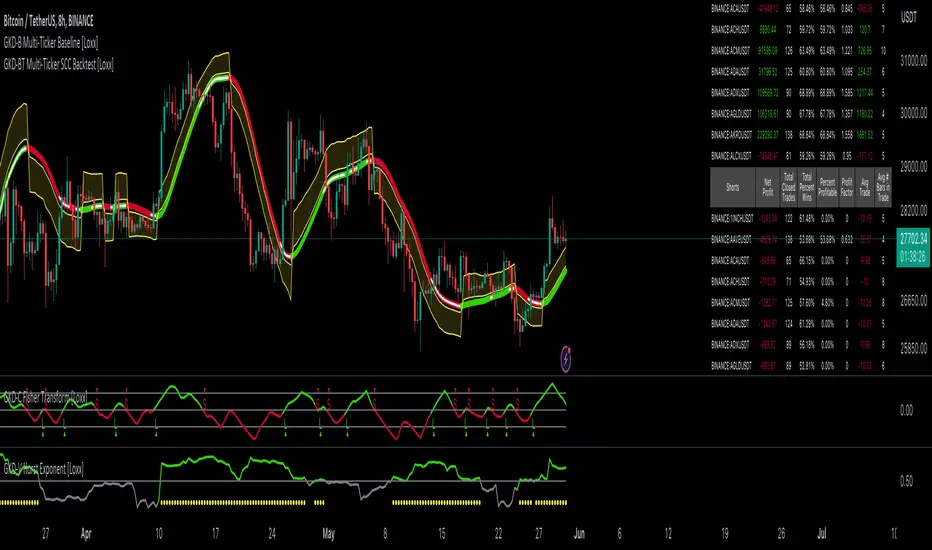
GKD-BT Multi-Ticker SCS Backtest [Loxx]The Giga Kaleidoscope GKD-BT Multi-Ticker SCS Backtest is a backtesting module included in Loxx's "Giga Kaleidoscope Modularized Trading System."
The Multi-Ticker SCS Backtest is a Solo Confirmation Simple backtest that allows traders to test single GKD-C confirmation indicators across 1-10 tickers. The purpose of this backtest is to enable traders to quickly evaluate GKD-C across hundreds of tickers within 30-60 minutes.
The backtest module supports testing with 1 take profit and 1 stop loss. It also offers the option to limit testing to a specific date range, allowing simulated forward testing using historical data. This backtest module only includes standard long and short signals. Additionally, users can choose to display or hide a trading panel that provides relevant information about the backtest, statistics, and the current trade. Traders can also select a highlighting treshold for Total Percent Wins and Percent Profitable, and Profit Factor.
To use this indicator:
1. Select the "Multi-ticker" option in the GKD-C Confirmation indicator.
2. Import 1-10 tickers into the GKD-C Confirmation indicator.
3. Import the same 1-10 indicators into the GKD-BT Multi-Ticker SCS Backtest.
4. Import the value "Input into NEW GKD-BT Multi-ticker Backtest" from the GKD-C Confirmation indicator into the GKD-BT Multi-Ticker SCS Backtest.
5. When importing tickers, ensure that you import the same type of tickers for all 1-10 tickers. For example, test only FX or Cryptocurrency or Stocks. Do not combine different tradable asset types.
6. Make sure that your chart is set to a ticker that corresponds to the tradable asset type. For cryptocurrency testing, set the chart to BTCUSDT. For Forex testing, set the chart to EURUSD.
This backtest includes the following metrics:
1. Net profit: Overall profit or loss achieved.
2. Total Closed Trades: Total number of closed trades, both winning and losing.
3. Total Percent Wins: Total wins, whether long or short, for the selected time interval regardless of commissions and other profit-modifying addons.
4. Percent Profitable: Total wins, whether long or short, that are also profitable, taking commissions into account.
5. Profit Factor: The ratio of gross profits to gross losses, indicating how much money the strategy made for every unit of money it lost.
6. Average Profit per Trade: The average gain or loss per trade, calculated by dividing the net profit by the total number of closed trades.
7. Average Number of Bars in Trade: The average number of bars that elapsed during trades for all closed trades.
Summary of notable settings:
Input Tickers separated by commas: Allows the user to input tickers separated by commas, specifying the symbols or tickers of financial instruments used in the backtest. The tickers should follow the format "EXCHANGE:TICKER" (e.g., "NASDAQ:AAPL, NYSE:MSFT").
Import GKD-C: Imports the "GKD-C" source, which provides signals or data for the backtest.
Initial Capital: Represents the starting account balance for the backtest, denominated in the base currency of the trading account.
Order Size: Determines the quantity of contracts traded in each trade.
Order Type: Specifies the type of order used in the backtest, either "Contracts" or "% Equity."
Commission: Represents the commission per order or transaction cost incurred in each trade.
**the backtest data rendered to the chart above uses $5 commission per trade and 10% equity per trade with $1 million initial capital. Each backtest result for each ticker assumes these same inputs. The results are NOT cumulative, they are separate and isolate per ticker and trading side, long or short**
Volatility Types included
The GKD system utilizes volatility-based take profits and stop losses. Each take profit and stop loss is calculated as a multiple of volatility. You can change the values of the multipliers in the settings as well.
This module includes 17 types of volatility:
Close-to-Close
Parkinson
Garman-Klass
Rogers-Satchell
Yang-Zhang
Garman-Klass-Yang-Zhang
Exponential Weighted Moving Average
Standard Deviation of Log Returns
Pseudo GARCH(2,2)
Average True Range
True Range Double
Standard Deviation
Adaptive Deviation
Median Absolute Deviation
Efficiency-Ratio Adaptive ATR
Mean Absolute Deviation
Static Percent
Various volatility estimators and indicators that investors and traders can use to measure the dispersion or volatility of a financial instrument's price. Each estimator has its strengths and weaknesses, and the choice of estimator should depend on the specific needs and circumstances of the user.
Close-to-Close
Close-to-Close volatility is a classic and widely used volatility measure, sometimes referred to as historical volatility.
Volatility is an indicator of the speed of a stock price change. A stock with high volatility is one where the price changes rapidly and with a larger amplitude. The more volatile a stock is, the riskier it is.
Close-to-close historical volatility is calculated using only a stock's closing prices. It is the simplest volatility estimator. However, in many cases, it is not precise enough. Stock prices could jump significantly during a trading session and return to the opening value at the end. That means that a considerable amount of price information is not taken into account by close-to-close volatility.
Despite its drawbacks, Close-to-Close volatility is still useful in cases where the instrument doesn't have intraday prices. For example, mutual funds calculate their net asset values daily or weekly, and thus their prices are not suitable for more sophisticated volatility estimators.
Parkinson
Parkinson volatility is a volatility measure that uses the stock’s high and low price of the day.
The main difference between regular volatility and Parkinson volatility is that the latter uses high and low prices for a day, rather than only the closing price. This is useful as close-to-close prices could show little difference while large price movements could have occurred during the day. Thus, Parkinson's volatility is considered more precise and requires less data for calculation than close-to-close volatility.
One drawback of this estimator is that it doesn't take into account price movements after the market closes. Hence, it systematically undervalues volatility. This drawback is addressed in the Garman-Klass volatility estimator.
Garman-Klass
Garman-Klass is a volatility estimator that incorporates open, low, high, and close prices of a security.
Garman-Klass volatility extends Parkinson's volatility by taking into account the opening and closing prices. As markets are most active during the opening and closing of a trading session, it makes volatility estimation more accurate.
Garman and Klass also assumed that the process of price change follows a continuous diffusion process (Geometric Brownian motion). However, this assumption has several drawbacks. The method is not robust for opening jumps in price and trend movements.
Despite its drawbacks, the Garman-Klass estimator is still more effective than the basic formula since it takes into account not only the price at the beginning and end of the time interval but also intraday price extremes.
Researchers Rogers and Satchell have proposed a more efficient method for assessing historical volatility that takes into account price trends. See Rogers-Satchell Volatility for more detail.
Rogers-Satchell
Rogers-Satchell is an estimator for measuring the volatility of securities with an average return not equal to zero.
Unlike Parkinson and Garman-Klass estimators, Rogers-Satchell incorporates a drift term (mean return not equal to zero). As a result, it provides better volatility estimation when the underlying is trending.
The main disadvantage of this method is that it does not take into account price movements between trading sessions. This leads to an underestimation of volatility since price jumps periodically occur in the market precisely at the moments between sessions.
A more comprehensive estimator that also considers the gaps between sessions was developed based on the Rogers-Satchel formula in the 2000s by Yang-Zhang. See Yang Zhang Volatility for more detail.
Yang-Zhang
Yang Zhang is a historical volatility estimator that handles both opening jumps and the drift and has a minimum estimation error.
Yang-Zhang volatility can be thought of as a combination of the overnight (close-to-open volatility) and a weighted average of the Rogers-Satchell volatility and the day’s open-to-close volatility. It is considered to be 14 times more efficient than the close-to-close estimator.
Garman-Klass-Yang-Zhang
Garman-Klass-Yang-Zhang (GKYZ) volatility estimator incorporates the returns of open, high, low, and closing prices in its calculation.
GKYZ volatility estimator takes into account overnight jumps but not the trend, i.e., it assumes that the underlying asset follows a Geometric Brownian Motion (GBM) process with zero drift. Therefore, the GKYZ volatility estimator tends to overestimate the volatility when the drift is different from zero. However, for a GBM process, this estimator is eight times more efficient than the close-to-close volatility estimator.
Exponential Weighted Moving Average
The Exponentially Weighted Moving Average (EWMA) is a quantitative or statistical measure used to model or describe a time series. The EWMA is widely used in finance, with the main applications being technical analysis and volatility modeling.
The moving average is designed such that older observations are given lower weights. The weights decrease exponentially as the data point gets older – hence the name exponentially weighted.
The only decision a user of the EWMA must make is the parameter lambda. The parameter decides how important the current observation is in the calculation of the EWMA. The higher the value of lambda, the more closely the EWMA tracks the original time series.
Standard Deviation of Log Returns
This is the simplest calculation of volatility. It's the standard deviation of ln(close/close(1)).
Pseudo GARCH(2,2)
This is calculated using a short- and long-run mean of variance multiplied by ?.
?avg(var;M) + (1 ? ?) avg(var;N) = 2?var/(M+1-(M-1)L) + 2(1-?)var/(M+1-(M-1)L)
Solving for ? can be done by minimizing the mean squared error of estimation; that is, regressing L^-1var - avg(var; N) against avg(var; M) - avg(var; N) and using the resulting beta estimate as ?.
Average True Range
The average true range (ATR) is a technical analysis indicator, introduced by market technician J. Welles Wilder Jr. in his book New Concepts in Technical Trading Systems, that measures market volatility by decomposing the entire range of an asset price for that period.
The true range indicator is taken as the greatest of the following: current high less the current low; the absolute value of the current high less the previous close; and the absolute value of the current low less the previous close. The ATR is then a moving average, generally using 14 days, of the true ranges.
True Range Double
A special case of ATR that attempts to correct for volatility skew.
Standard Deviation
Standard deviation is a statistic that measures the dispersion of a dataset relative to its mean and is calculated as the square root of the variance. The standard deviation is calculated as the square root of variance by determining each data point's deviation relative to the mean. If the data points are further from the mean, there is a higher deviation within the data set; thus, the more spread out the data, the higher the standard deviation.
Adaptive Deviation
By definition, the Standard Deviation (STD, also represented by the Greek letter sigma ? or the Latin letter s) is a measure that is used to quantify the amount of variation or dispersion of a set of data values. In technical analysis, we usually use it to measure the level of current volatility.
Standard Deviation is based on Simple Moving Average calculation for mean value. This version of standard deviation uses the properties of EMA to calculate what can be called a new type of deviation, and since it is based on EMA, we can call it EMA deviation. Additionally, Perry Kaufman's efficiency ratio is used to make it adaptive (since all EMA type calculations are nearly perfect for adapting).
The difference when compared to the standard is significant--not just because of EMA usage, but the efficiency ratio makes it a "bit more logical" in very volatile market conditions.
Median Absolute Deviation
The median absolute deviation is a measure of statistical dispersion. Moreover, the MAD is a robust statistic, being more resilient to outliers in a data set than the standard deviation. In the standard deviation, the distances from the mean are squared, so large deviations are weighted more heavily, and thus outliers can heavily influence it. In the MAD, the deviations of a small number of outliers are irrelevant.
Because the MAD is a more robust estimator of scale than the sample variance or standard deviation, it works better with distributions without a mean or variance, such as the Cauchy distribution.
For this indicator, a manual recreation of the quantile function in Pine Script is used. This is so users have a full inside view into how this is calculated.
Efficiency-Ratio Adaptive ATR
Average True Range (ATR) is a widely used indicator for many occasions in technical analysis. It is calculated as the RMA of the true range. This version adds a "twist": it uses Perry Kaufman's Efficiency Ratio to calculate adaptive true range.
Mean Absolute Deviation
The mean absolute deviation (MAD) is a measure of variability that indicates the average distance between observations and their mean. MAD uses the original units of the data, which simplifies interpretation. Larger values signify that the data points spread out further from the average. Conversely, lower values correspond to data points bunching closer to it. The mean absolute deviation is also known as the mean deviation and average absolute deviation.
This definition of the mean absolute deviation sounds similar to the standard deviation (SD). While both measure variability, they have different calculations. In recent years, some proponents of MAD have suggested that it replace the SD as the primary measure because it is a simpler concept that better fits real life.
█ Giga Kaleidoscope Modularized Trading System
Core components of an NNFX algorithmic trading strategy
The NNFX algorithm is built on the principles of trend, momentum, and volatility. There are six core components in the NNFX trading algorithm:
1. Volatility - price volatility; e.g., Average True Range, True Range Double, Close-to-Close, etc.
2. Baseline - a moving average to identify price trend
3. Confirmation 1 - a technical indicator used to identify trends
4. Confirmation 2 - a technical indicator used to identify trends
5. Continuation - a technical indicator used to identify trends
6. Volatility/Volume - a technical indicator used to identify volatility/volume breakouts/breakdown
7. Exit - a technical indicator used to determine when a trend is exhausted
8. Metamorphosis - a technical indicator that produces a compound signal from the combination of other GKD indicators*
*(not part of the NNFX algorithm)
What is Volatility in the NNFX trading system?
In the NNFX (No Nonsense Forex) trading system, ATR (Average True Range) is typically used to measure the volatility of an asset. It is used as a part of the system to help determine the appropriate stop loss and take profit levels for a trade. ATR is calculated by taking the average of the true range values over a specified period.
True range is calculated as the maximum of the following values:
-Current high minus the current low
-Absolute value of the current high minus the previous close
-Absolute value of the current low minus the previous close
ATR is a dynamic indicator that changes with changes in volatility. As volatility increases, the value of ATR increases, and as volatility decreases, the value of ATR decreases. By using ATR in NNFX system, traders can adjust their stop loss and take profit levels according to the volatility of the asset being traded. This helps to ensure that the trade is given enough room to move, while also minimizing potential losses.
Other types of volatility include True Range Double (TRD), Close-to-Close, and Garman-Klass
What is a Baseline indicator?
The baseline is essentially a moving average, and is used to determine the overall direction of the market.
The baseline in the NNFX system is used to filter out trades that are not in line with the long-term trend of the market. The baseline is plotted on the chart along with other indicators, such as the Moving Average (MA), the Relative Strength Index (RSI), and the Average True Range (ATR).
Trades are only taken when the price is in the same direction as the baseline. For example, if the baseline is sloping upwards, only long trades are taken, and if the baseline is sloping downwards, only short trades are taken. This approach helps to ensure that trades are in line with the overall trend of the market, and reduces the risk of entering trades that are likely to fail.
By using a baseline in the NNFX system, traders can have a clear reference point for determining the overall trend of the market, and can make more informed trading decisions. The baseline helps to filter out noise and false signals, and ensures that trades are taken in the direction of the long-term trend.
What is a Confirmation indicator?
Confirmation indicators are technical indicators that are used to confirm the signals generated by primary indicators. Primary indicators are the core indicators used in the NNFX system, such as the Average True Range (ATR), the Moving Average (MA), and the Relative Strength Index (RSI).
The purpose of the confirmation indicators is to reduce false signals and improve the accuracy of the trading system. They are designed to confirm the signals generated by the primary indicators by providing additional information about the strength and direction of the trend.
Some examples of confirmation indicators that may be used in the NNFX system include the Bollinger Bands, the MACD (Moving Average Convergence Divergence), and the MACD Oscillator. These indicators can provide information about the volatility, momentum, and trend strength of the market, and can be used to confirm the signals generated by the primary indicators.
In the NNFX system, confirmation indicators are used in combination with primary indicators and other filters to create a trading system that is robust and reliable. By using multiple indicators to confirm trading signals, the system aims to reduce the risk of false signals and improve the overall profitability of the trades.
What is a Continuation indicator?
In the NNFX (No Nonsense Forex) trading system, a continuation indicator is a technical indicator that is used to confirm a current trend and predict that the trend is likely to continue in the same direction. A continuation indicator is typically used in conjunction with other indicators in the system, such as a baseline indicator, to provide a comprehensive trading strategy.
What is a Volatility/Volume indicator?
Volume indicators, such as the On Balance Volume (OBV), the Chaikin Money Flow (CMF), or the Volume Price Trend (VPT), are used to measure the amount of buying and selling activity in a market. They are based on the trading volume of the market, and can provide information about the strength of the trend. In the NNFX system, volume indicators are used to confirm trading signals generated by the Moving Average and the Relative Strength Index. Volatility indicators include Average Direction Index, Waddah Attar, and Volatility Ratio. In the NNFX trading system, volatility is a proxy for volume and vice versa.
By using volume indicators as confirmation tools, the NNFX trading system aims to reduce the risk of false signals and improve the overall profitability of trades. These indicators can provide additional information about the market that is not captured by the primary indicators, and can help traders to make more informed trading decisions. In addition, volume indicators can be used to identify potential changes in market trends and to confirm the strength of price movements.
What is an Exit indicator?
The exit indicator is used in conjunction with other indicators in the system, such as the Moving Average (MA), the Relative Strength Index (RSI), and the Average True Range (ATR), to provide a comprehensive trading strategy.
The exit indicator in the NNFX system can be any technical indicator that is deemed effective at identifying optimal exit points. Examples of exit indicators that are commonly used include the Parabolic SAR, the Average Directional Index (ADX), and the Chandelier Exit.
The purpose of the exit indicator is to identify when a trend is likely to reverse or when the market conditions have changed, signaling the need to exit a trade. By using an exit indicator, traders can manage their risk and prevent significant losses.
In the NNFX system, the exit indicator is used in conjunction with a stop loss and a take profit order to maximize profits and minimize losses. The stop loss order is used to limit the amount of loss that can be incurred if the trade goes against the trader, while the take profit order is used to lock in profits when the trade is moving in the trader's favor.
Overall, the use of an exit indicator in the NNFX trading system is an important component of a comprehensive trading strategy. It allows traders to manage their risk effectively and improve the profitability of their trades by exiting at the right time.
What is an Metamorphosis indicator?
The concept of a metamorphosis indicator involves the integration of two or more GKD indicators to generate a compound signal. This is achieved by evaluating the accuracy of each indicator and selecting the signal from the indicator with the highest accuracy. As an illustration, let's consider a scenario where we calculate the accuracy of 10 indicators and choose the signal from the indicator that demonstrates the highest accuracy.
The resulting output from the metamorphosis indicator can then be utilized in a GKD-BT backtest by occupying a slot that aligns with the purpose of the metamorphosis indicator. The slot can be a GKD-B, GKD-C, or GKD-E slot, depending on the specific requirements and objectives of the indicator. This allows for seamless integration and utilization of the compound signal within the GKD-BT framework.
How does Loxx's GKD (Giga Kaleidoscope Modularized Trading System) implement the NNFX algorithm outlined above?
Loxx's GKD v2.0 system has five types of modules (indicators/strategies). These modules are:
1. GKD-BT - Backtesting module (Volatility, Number 1 in the NNFX algorithm)
2. GKD-B - Baseline module (Baseline and Volatility/Volume, Numbers 1 and 2 in the NNFX algorithm)
3. GKD-C - Confirmation 1/2 and Continuation module (Confirmation 1/2 and Continuation, Numbers 3, 4, and 5 in the NNFX algorithm)
4. GKD-V - Volatility/Volume module (Confirmation 1/2, Number 6 in the NNFX algorithm)
5. GKD-E - Exit module (Exit, Number 7 in the NNFX algorithm)
6. GKD-M - Metamorphosis module (Metamorphosis, Number 8 in the NNFX algorithm, but not part of the NNFX algorithm)
(additional module types will added in future releases)
Each module interacts with every module by passing data to A backtest module wherein the various components of the GKD system are combined to create a trading signal.
That is, the Baseline indicator passes its data to Volatility/Volume. The Volatility/Volume indicator passes its values to the Confirmation 1 indicator. The Confirmation 1 indicator passes its values to the Confirmation 2 indicator. The Confirmation 2 indicator passes its values to the Continuation indicator. The Continuation indicator passes its values to the Exit indicator, and finally, the Exit indicator passes its values to the Backtest strategy.
This chaining of indicators requires that each module conform to Loxx's GKD protocol, therefore allowing for the testing of every possible combination of technical indicators that make up the six components of the NNFX algorithm.
What does the application of the GKD trading system look like?
Example trading system:
Backtest: Multi-Ticker SCS Backtest
Baseline: Hull Moving Average
Volatility/Volume: Hurst Exponent
Confirmation 1: Kase Peak Oscillator
Confirmation 2: uf2018
Continuation: Vortex
Exit: Rex Oscillator
Metamorphosis: Baseline Optimizer
Each GKD indicator is denoted with a module identifier of either: GKD-BT, GKD-B, GKD-C, GKD-V, GKD-M, or GKD-E. This allows traders to understand to which module each indicator belongs and where each indicator fits into the GKD system.
█ Giga Kaleidoscope Modularized Trading System Signals
Standard Entry
1. GKD-C Confirmation gives signal
2. Baseline agrees
3. Price inside Goldie Locks Zone Minimum
4. Price inside Goldie Locks Zone Maximum
5. Confirmation 2 agrees
6. Volatility/Volume agrees
1-Candle Standard Entry
1a. GKD-C Confirmation gives signal
2a. Baseline agrees
3a. Price inside Goldie Locks Zone Minimum
4a. Price inside Goldie Locks Zone Maximum
Next Candle
1b. Price retraced
2b. Baseline agrees
3b. Confirmation 1 agrees
4b. Confirmation 2 agrees
5b. Volatility/Volume agrees
Baseline Entry
1. GKD-B Basline gives signal
2. Confirmation 1 agrees
3. Price inside Goldie Locks Zone Minimum
4. Price inside Goldie Locks Zone Maximum
5. Confirmation 2 agrees
6. Volatility/Volume agrees
7. Confirmation 1 signal was less than 'Maximum Allowable PSBC Bars Back' prior
1-Candle Baseline Entry
1a. GKD-B Baseline gives signal
2a. Confirmation 1 agrees
3a. Price inside Goldie Locks Zone Minimum
4a. Price inside Goldie Locks Zone Maximum
5a. Confirmation 1 signal was less than 'Maximum Allowable PSBC Bars Back' prior
Next Candle
1b. Price retraced
2b. Baseline agrees
3b. Confirmation 1 agrees
4b. Confirmation 2 agrees
5b. Volatility/Volume agrees
Volatility/Volume Entry
1. GKD-V Volatility/Volume gives signal
2. Confirmation 1 agrees
3. Price inside Goldie Locks Zone Minimum
4. Price inside Goldie Locks Zone Maximum
5. Confirmation 2 agrees
6. Baseline agrees
7. Confirmation 1 signal was less than 7 candles prior
1-Candle Volatility/Volume Entry
1a. GKD-V Volatility/Volume gives signal
2a. Confirmation 1 agrees
3a. Price inside Goldie Locks Zone Minimum
4a. Price inside Goldie Locks Zone Maximum
5a. Confirmation 1 signal was less than 'Maximum Allowable PSVVC Bars Back' prior
Next Candle
1b. Price retraced
2b. Volatility/Volume agrees
3b. Confirmation 1 agrees
4b. Confirmation 2 agrees
5b. Baseline agrees
Confirmation 2 Entry
1. GKD-C Confirmation 2 gives signal
2. Confirmation 1 agrees
3. Price inside Goldie Locks Zone Minimum
4. Price inside Goldie Locks Zone Maximum
5. Volatility/Volume agrees
6. Baseline agrees
7. Confirmation 1 signal was less than 7 candles prior
1-Candle Confirmation 2 Entry
1a. GKD-C Confirmation 2 gives signal
2a. Confirmation 1 agrees
3a. Price inside Goldie Locks Zone Minimum
4a. Price inside Goldie Locks Zone Maximum
5a. Confirmation 1 signal was less than 'Maximum Allowable PSC2C Bars Back' prior
Next Candle
1b. Price retraced
2b. Confirmation 2 agrees
3b. Confirmation 1 agrees
4b. Volatility/Volume agrees
5b. Baseline agrees
PullBack Entry
1a. GKD-B Baseline gives signal
2a. Confirmation 1 agrees
3a. Price is beyond 1.0x Volatility of Baseline
Next Candle
1b. Price inside Goldie Locks Zone Minimum
2b. Price inside Goldie Locks Zone Maximum
3b. Confirmation 1 agrees
4b. Confirmation 2 agrees
5b. Volatility/Volume agrees
Continuation Entry
1. Standard Entry, 1-Candle Standard Entry, Baseline Entry, 1-Candle Baseline Entry, Volatility/Volume Entry, 1-Candle Volatility/Volume Entry, Confirmation 2 Entry, 1-Candle Confirmation 2 Entry, or Pullback entry triggered previously
2. Baseline hasn't crossed since entry signal trigger
4. Confirmation 1 agrees
5. Baseline agrees
6. Confirmation 2 agrees
█ Connecting to Backtests
All GKD indicators are chained indicators meaning you export the value of the indicators to specialized backtest to creat your GKD trading system. Each indicator contains a proprietary signal generation algo that will only work with GKD backtests. You can find these backtests using the links below.
GKD-BT Giga Confirmation Stack Backtest
GKD-BT Giga Stacks Backtest
GKD-BT Full Giga Kaleidoscope Backtest
GKD-BT Solo Confirmation Super Complex Backtest
GKD-BT Solo Confirmation Complex Backtest
GKD-BT Solo Confirmation Simple Backtest
GKD-M Baseline Optimizer
GKD-M Accuracy Alchemist
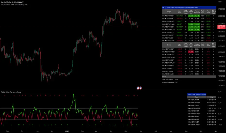
GKD-C Adaptive-Lookback Variety RSI [Loxx]Giga Kaleidoscope GKD-C Adaptive-Lookback Variety RSI is a Confirmation module included in Loxx's "Giga Kaleidoscope Modularized Trading System".
█ GKD-C Adaptive-Lookback Variety RSI
What is the Adaptive Lookback Period?
The adaptive lookback period is a technique used in technical analysis to adjust the period of an indicator based on changes in market conditions. This technique is particularly useful in volatile or rapidly changing markets where a fixed period may not be optimal for detecting trends or signals.
The concept of the adaptive lookback period is relatively simple. By adjusting the lookback period based on changes in market conditions, traders can more accurately identify trends and signals. This can help traders to enter and exit trades at the right time and improve the profitability of their trading strategies.
The adaptive lookback period works by identifying potential swing points in the market. Once these points are identified, the lookback period is calculated based on the number of swings and a speed parameter. The swing count parameter determines the number of swings that must occur before the lookback period is adjusted. The speed parameter controls the rate at which the lookback period is adjusted, with higher values indicating a more rapid adjustment.
The adaptive lookback period can be applied to a wide range of technical indicators, including moving averages, oscillators, and trendlines. By adjusting the period of these indicators based on changes in market conditions, traders can reduce the impact of noise and false signals, leading to more profitable trades.
In summary, the adaptive lookback period is a powerful technique for traders and analysts looking to optimize their technical indicators. By adjusting the period based on changes in market conditions, traders can more accurately identify trends and signals, leading to more profitable trades. While there are various ways to implement the adaptive lookback period, the basic concept remains the same, and traders can adapt and customize the technique to suit their individual needs and trading styles.
This indicator includes 10 types of RSI
1. Regular RSI
2. Slow RSI
3. Ehlers Smoothed RSI
4. Cutler's RSI
5. Rapid RSI
6. Harris' RSI
7. RSI DEMA
8. RSI TEMA
9. RSI T3
10. Jurik RSX
Regular RSI
The Relative Strength Index (RSI) is a widely used technical indicator in the field of financial market analysis. Developed by J. Welles Wilder Jr. in 1978, the RSI is a momentum oscillator that measures the speed and change of price movements. It helps traders identify potential trend reversals, overbought, and oversold conditions in a market.
The RSI is calculated based on the average gains and losses of an asset over a specified period, typically 14 days. The formula for calculating the RSI is as follows:
RSI = 100 - (100 / (1 + RS))
Where:
RS (Relative Strength) = Average gain over the specified period / Average loss over the specified period
The RSI ranges from 0 to 100, with values above 70 generally considered overbought (potentially indicating that the asset is overvalued and may experience a price decline) and values below 30 considered oversold (potentially indicating that the asset is undervalued and may experience a price increase).
Slow RSI
Slow RSI is a modified version of the Relative Strength Index (RSI) indicator that aims to provide a smoother, more consistent signal than the traditional RSI. The Slow RSI is designed to be less sensitive to sudden price movements, which can cause false signals.
To calculate Slow RSI, we first calculate the up and down values, just like in traditional RSI and Ehlers RSI. The up and down values are calculated by comparing the current price to the previous price, and then adding up the positive and negative differences.
Next, we calculate the Slow RSI value using the formula:
SlowRSI = 100 * up / (up + dn)
where "up" and "dn" are the total positive and negative differences, respectively.
This formula is similar to the one used in traditional RSI, but the dynamic lookback period based on the average of the up and down values is used to smooth out the signal.
Finally, we apply smoothing to the Slow RSI value by taking an exponential moving average (EMA) of the Slow RSI values over a specified period. This EMA helps to reduce the impact of sudden price movements and provide a smoother, more consistent signal over time.
Ehler's Smoothed RSI
Ehlers RSI is a modified version of the Relative Strength Index (RSI) indicator created by John Ehlers, a well-known technical analyst and author. The purpose of Ehlers RSI is to reduce lag and improve the responsiveness of the traditional RSI indicator.
To calculate Ehlers RSI, we first smooth the prices by taking a weighted average of the current price and the two previous prices. This smoothing helps to reduce noise in the data and produce a more accurate signal.
Next, we calculate the up and down values differently than in traditional RSI. In traditional RSI, the up and down values are based on the difference between the current price and the previous price. In Ehlers RSI, the up and down values are based on the difference between the current price and the price two bars ago. This approach helps to reduce lag and produce a more responsive indicator.
Finally, we calculate Ehlers RSI using the formula:
EhlersRSI = 50 * (up - down) / (up + down) + 50
The result is a more timely signal that can help traders identify potential trends and reversals in the market. However, as with any technical indicator, Ehlers RSI should be used in conjunction with other analysis tools and should not be relied on as the sole basis for trading decisions.
Cutler's RSI
Cutler's RSI (Relative Strength Index) is a variation of the traditional RSI, a popular technical analysis indicator used to measure the speed and change of price movements. The main difference between Cutler's RSI and the traditional RSI is the calculation method used to smooth the data. While the traditional RSI uses an exponential moving average (EMA) to smooth the data, Cutler's RSI uses a simple moving average (SMA).
Here's the formula for Cutler's RSI:
1. Calculate the price change: Price Change = Current Price - Previous Price
2. Calculate the average gain and average loss over a specified period (usually 14 days):
If Price Change > 0, add it to the total gains.
If Price Change < 0, add the absolute value to the total losses.
3. Calculate the average gain and average loss by dividing the totals by the specified period: Average Gain = Total Gains / Period, Average Loss = Total Losses / Period
4. Calculate the Relative Strength (RS): RS = Average Gain / Average Loss
5. Calculate Cutler's RSI: Cutler's RSI = 100 - (100 / (1 + RS))
Cutler's RSI is not necessarily better than the regular RSI; it's just a different variation of the traditional RSI that uses a simple moving average (SMA) instead of an exponential moving average (EMA) quantifiedstrategies.com. The main advantage of Cutler's RSI is that it is not data length dependent, meaning it returns consistent results regardless of the length of the period, or the starting point within a data file quantifiedstrategies.com.
However, it's worth noting that Cutler's RSI does not necessarily outperform the traditional RSI. In fact, backtests reveal that Cutler's RSI is no improvement compared to Wilder's RSI quantifiedstrategies.com. Additionally, using an SMA instead of an EMA in Cutler's RSI may result in the loss of the "believed" advantage of weighting the most recent price action aaii.com.
Both Cutler's RSI and the traditional RSI can be used to identify overbought/oversold levels, support and resistance, spot divergences for possible reversals, and confirm the signals from other indicators investopedia.com. Ultimately, the choice between Cutler's RSI and the traditional RSI depends on personal preference and the specific trading strategy being employed.
Rapid RSI
Rapid RSI is a technical analysis indicator that is a modified version of the Relative Strength Index (RSI). It was developed by Andrew Cardwell and was first introduced in the October 2006 issue of Technical Analysis of Stocks & Commodities magazine.
The Rapid RSI improves upon the regular RSI by modifying the way the average gains and losses are calculated. Here's a general breakdown of the Rapid RSI calculation:
1. Calculate the upward change (when the price has increased) and the downward change (when the price has decreased) for each period.
2. Calculate the simple moving average (SMA) of the upward changes and the SMA of the downward changes over the specified period.
3. Divide the SMA of the upward changes by the SMA of the downward changes to get the relative strength (RS).
4. Calculate the Rapid RSI by transforming the relative strength (RS) into a value ranging from 0 to 100.
By using the simple moving average (SMA) instead of the slow exponential moving average (RMA) as in the regular RSI, the Rapid RSI tends to be more responsive to recent price changes. This can help traders identify overbought and oversold conditions more quickly, potentially leading to earlier entry and exit points. However, it is important to note that a faster indicator may also produce more false signals.
Harris' RSI
Harris RSI (Relative Strength Index) is a technical indicator used in financial analysis to measure the strength or weakness of a security over time. It was developed by Larry Harris in 1986 as an alternative to the traditional RSI, which measures the price change of a security over a given period.
The Harris RSI uses a slightly different formula from the traditional RSI, but it is based on the same principles. It calculates the ratio of the average gain to the average loss over a specified period, typically 14 days. The result is then plotted on a scale of 0 to 100, with high values indicating overbought conditions and low values indicating oversold conditions.
The Harris RSI is believed to be more responsive to short-term price movements than the traditional RSI, making it useful for traders who are looking for quick trading opportunities. However, like any technical indicator, it should be used in conjunction with other forms of analysis to make informed trading decisions.
The calculation of the Harris RSI involves several steps:
1. Calculate the price change over the specified period (usually 14 days) using the following formula:
Price Change = Close Price - Prior Close Price
2. Calculate the average gain and average loss over the same period, using separate formulas for each:
Average Gain = (Sum of Gains over the Period) / Period
Average Loss = (Sum of Losses over the Period) / Period
Gains are calculated as the sum of all positive price changes over the period, while losses are calculated as the sum of all negative price changes over the period.
3. Calculate the Relative Strength (RS) as the ratio of the Average Gain to the Average Loss:
RS = Average Gain / Average Loss
4. Calculate the Harris RSI using the following formula:
Harris RSI = 100 - (100 / (1 + RS))
The resulting Harris RSI value is a number between 0 and 100, which is plotted on a chart to identify overbought or oversold conditions in the security. A value above 70 is generally considered overbought, while a value below 30 is generally considered oversold.
DEMA RSI
DEMA RSI is a variation of the Relative Strength Index (RSI) technical indicator that incorporates the Double Exponential Moving Average (DEMA) for smoothing. Like the regular RSI, the DEMA RSI is a momentum oscillator used to measure the speed and change of price movements, and it ranges from 0 to 100. Readings below 30 typically indicate oversold conditions, while readings above 70 indicate overbought conditions.
The DEMA RSI aims to improve upon the regular RSI by addressing its limitations, such as lag and false signals. By using the DEMA, a more responsive and faster RSI can be achieved. Here's a general breakdown of the DEMA RSI calculation:
1. Calculate the price change for each period, as well as the absolute value of the change.
2. Apply the DEMA smoothing technique to both the price change and its absolute value, separately. This involves calculating two sets of exponential moving averages and combining them to create a double-weighted moving average with reduced lag.
3. Divide the smoothed price change by the smoothed absolute value of the price change.
4. Transform the result into a value ranging from 0 to 100 to obtain the DEMA RSI.
The DEMA RSI is considered an improvement over the regular RSI because it provides faster and more responsive signals. This can help traders identify overbought and oversold conditions more accurately and potentially avoid false signals.
In summary, the main advantages of these RSI variations over the regular RSI are their ability to reduce noise, provide smoother lines, and be more responsive to price changes. This can lead to more accurate signals and fewer false positives in different market conditions.
TEMA RSI
TEMA RSI is a variation of the Relative Strength Index (RSI) technical indicator that incorporates the Triple Exponential Moving Average (TEMA) for smoothing. Like the regular RSI, the TEMA RSI is a momentum oscillator used to measure the speed and change of price movements, and it ranges from 0 to 100. Readings below 30 typically indicate oversold conditions, while readings above 70 indicate overbought conditions.
The TEMA RSI aims to improve upon the regular RSI by addressing its limitations, such as lag and false signals. By using the TEMA, a more responsive and faster RSI can be achieved. Here's a general breakdown of the TEMA RSI calculation:
1. Calculate the price change for each period, as well as the absolute value of the change.
2. Apply the TEMA smoothing technique to both the price change and its absolute value, separately. This involves calculating two sets of exponential moving averages and combining them to create a double-weighted moving average with reduced lag.
3. Divide the smoothed price change by the smoothed absolute value of the price change.
4. Transform the result into a value ranging from 0 to 100 to obtain the TEMA RSI.
The TEMA RSI is considered an improvement over the regular RSI because it provides faster and more responsive signals. This can help traders identify overbought and oversold conditions more accurately and potentially avoid false signals.
T3 RSI
T3 RSI is a variation of the Relative Strength Index (RSI) technical indicator that incorporates the Tilson T3 for smoothing. Like the regular RSI, the T3 RSI is a momentum oscillator used to measure the speed and change of price movements, and it ranges from 0 to 100. Readings below 30 typically indicate oversold conditions, while readings above 70 indicate overbought conditions.
The T3 RSI aims to improve upon the regular RSI by addressing its limitations, such as lag and false signals. By using the T3, a more responsive and faster RSI can be achieved. Here's a general breakdown of the T3 RSI calculation:
1. Calculate the price change for each period, as well as the absolute value of the change.
2. Apply the T3 smoothing technique to both the price change and its absolute value, separately. This involves calculating two sets of exponential moving averages and combining them to create a double-weighted moving average with reduced lag.
3. Divide the smoothed price change by the smoothed absolute value of the price change.
4. Transform the result into a value ranging from 0 to 100 to obtain the T3 RSI.
The T3 RSI is considered an improvement over the regular RSI because it provides faster and more responsive signals. This can help traders identify overbought and oversold conditions more accurately and potentially avoid false signals.
Jurik RSX
The Jurik RSX is a technical indicator developed by Mark Jurik to measure the momentum and strength of price movements in financial markets, such as stocks, commodities, and currencies. It is an advanced version of the traditional Relative Strength Index (RSI), designed to offer smoother and less lagging signals compared to the standard RSI.
The main advantage of the Jurik RSX is that it provides more accurate and timely signals for traders and analysts, thanks to its improved calculation methods that reduce noise and lag in the indicator's output. This enables better decision-making when analyzing market trends and potential trading opportunities.
What is Adaptive-Lookback Variety RSI
This indicator allows the user to select from 9 different RSI types and 33 source types. The various RSI types is enhanced by injecting an adaptive lookback period into the caculation making the RSI able to adaptive to differing market conditions.
Additional Features
This indicator allows you to select from 33 source types. They are as follows:
Close
Open
High
Low
Median
Typical
Weighted
Average
Average Median Body
Trend Biased
Trend Biased (Extreme)
HA Close
HA Open
HA High
HA Low
HA Median
HA Typical
HA Weighted
HA Average
HA Average Median Body
HA Trend Biased
HA Trend Biased (Extreme)
HAB Close
HAB Open
HAB High
HAB Low
HAB Median
HAB Typical
HAB Weighted
HAB Average
HAB Average Median Body
HAB Trend Biased
HAB Trend Biased (Extreme)
What are Heiken Ashi "better" candles?
Heiken Ashi "better" candles are a modified version of the standard Heiken Ashi candles, which are a popular charting technique used in technical analysis. Heiken Ashi candles help traders identify trends and potential reversal points by smoothing out price data and reducing market noise. The "better formula" was proposed by Sebastian Schmidt in an article published by BNP Paribas in Warrants & Zertifikate, a German magazine, in August 2004. The aim of this formula is to further improve the smoothing of the Heiken Ashi chart and enhance its effectiveness in identifying trends and reversals.
Standard Heiken Ashi candles are calculated using the following formulas:
Heiken Ashi Close = (Open + High + Low + Close) / 4
Heiken Ashi Open = (Previous Heiken Ashi Open + Previous Heiken Ashi Close) / 2
Heiken Ashi High = Max (High, Heiken Ashi Open, Heiken Ashi Close)
Heiken Ashi Low = Min (Low, Heiken Ashi Open, Heiken Ashi Close)
The "better formula" modifies the standard Heiken Ashi calculation by incorporating additional smoothing, which can help reduce noise and make it easier to identify trends and reversals. The modified formulas for Heiken Ashi "better" candles are as follows:
Better Heiken Ashi Close = (Open + High + Low + Close) / 4
Better Heiken Ashi Open = (Previous Better Heiken Ashi Open + Previous Better Heiken Ashi Close) / 2
Better Heiken Ashi High = Max (High, Better Heiken Ashi Open, Better Heiken Ashi Close)
Better Heiken Ashi Low = Min (Low, Better Heiken Ashi Open, Better Heiken Ashi Close)
Smoothing Factor = 2 / (N + 1), where N is the chosen period for smoothing
Smoothed Better Heiken Ashi Open = (Better Heiken Ashi Open * Smoothing Factor) + (Previous Smoothed Better Heiken Ashi Open * (1 - Smoothing Factor))
Smoothed Better Heiken Ashi Close = (Better Heiken Ashi Close * Smoothing Factor) + (Previous Smoothed Better Heiken Ashi Close * (1 - Smoothing Factor))
The smoothed Better Heiken Ashi Open and Close values are then used to calculate the smoothed Better Heiken Ashi High and Low values, resulting in "better" candles that provide a clearer representation of the market trend and potential reversal points.
It's important to note that, like any other technical analysis tool, Heiken Ashi "better" candles are not foolproof and should be used in conjunction with other indicators and analysis techniques to make well-informed trading decisions.
Heiken Ashi "better" candles, as mentioned previously, provide a clearer representation of market trends and potential reversal points by reducing noise and smoothing out price data. When using these candles in conjunction with other technical analysis tools and indicators, traders can gain valuable insights into market behavior and make more informed decisions.
To effectively use Heiken Ashi "better" candles in your trading strategy, consider the following tips:
Trend Identification: Heiken Ashi "better" candles can help you identify the prevailing trend in the market. When the majority of the candles are green (or another color, depending on your chart settings) and there are no or few lower wicks, it may indicate a strong uptrend. Conversely, when the majority of the candles are red (or another color) and there are no or few upper wicks, it may signal a strong downtrend.
Trend Reversals: Look for potential trend reversals when a change in the color of the candles occurs, especially when accompanied by longer wicks. For example, if a green candle with a long lower wick is followed by a red candle, it could indicate a bearish reversal. Similarly, a red candle with a long upper wick followed by a green candle may suggest a bullish reversal.
Support and Resistance: You can use Heiken Ashi "better" candles to identify potential support and resistance levels. When the candles are consistently moving in one direction and then suddenly change color with longer wicks, it could indicate the presence of a support or resistance level.
Stop-Loss and Take-Profit: Using Heiken Ashi "better" candles can help you manage risk by determining optimal stop-loss and take-profit levels. For instance, you can place your stop-loss below the low of the most recent green candle in an uptrend or above the high of the most recent red candle in a downtrend.
Confirming Signals: Heiken Ashi "better" candles should be used in conjunction with other technical indicators, such as moving averages, oscillators, or chart patterns, to confirm signals and improve the accuracy of your analysis.
In this implementation, you have the choice of AMA, KAMA, or T3 smoothing. These are as follows:
Kaufman Adaptive Moving Average (KAMA)
The Kaufman Adaptive Moving Average (KAMA) is a type of adaptive moving average used in technical analysis to smooth out price fluctuations and identify trends. The KAMA adjusts its smoothing factor based on the market's volatility, making it more responsive in volatile markets and smoother in calm markets. The KAMA is calculated using three different efficiency ratios that determine the appropriate smoothing factor for the current market conditions. These ratios are based on the noise level of the market, the speed at which the market is moving, and the length of the moving average. The KAMA is a popular choice among traders who prefer to use adaptive indicators to identify trends and potential reversals.
Adaptive Moving Average
The Adaptive Moving Average (AMA) is a type of moving average that adjusts its sensitivity to price movements based on market conditions. It uses a ratio between the current price and the highest and lowest prices over a certain lookback period to determine its level of smoothing. The AMA can help reduce lag and increase responsiveness to changes in trend direction, making it useful for traders who want to follow trends while avoiding false signals. The AMA is calculated by multiplying a smoothing constant with the difference between the current price and the previous AMA value, then adding the result to the previous AMA value.
T3
The T3 moving average is a type of technical indicator used in financial analysis to identify trends in price movements. It is similar to the Exponential Moving Average (EMA) and the Double Exponential Moving Average (DEMA), but uses a different smoothing algorithm.
The T3 moving average is calculated using a series of exponential moving averages that are designed to filter out noise and smooth the data. The resulting smoothed data is then weighted with a non-linear function to produce a final output that is more responsive to changes in trend direction.
The T3 moving average can be customized by adjusting the length of the moving average, as well as the weighting function used to smooth the data. It is commonly used in conjunction with other technical indicators as part of a larger trading strategy.
█ Giga Kaleidoscope Modularized Trading System
Core components of an NNFX algorithmic trading strategy
The NNFX algorithm is built on the principles of trend, momentum, and volatility. There are six core components in the NNFX trading algorithm:
1. Volatility - price volatility; e.g., Average True Range, True Range Double, Close-to-Close, etc.
2. Baseline - a moving average to identify price trend
3. Confirmation 1 - a technical indicator used to identify trends
4. Confirmation 2 - a technical indicator used to identify trends
5. Continuation - a technical indicator used to identify trends
6. Volatility/Volume - a technical indicator used to identify volatility/volume breakouts/breakdown
7. Exit - a technical indicator used to determine when a trend is exhausted
What is Volatility in the NNFX trading system?
In the NNFX (No Nonsense Forex) trading system, ATR (Average True Range) is typically used to measure the volatility of an asset. It is used as a part of the system to help determine the appropriate stop loss and take profit levels for a trade. ATR is calculated by taking the average of the true range values over a specified period.
True range is calculated as the maximum of the following values:
-Current high minus the current low
-Absolute value of the current high minus the previous close
-Absolute value of the current low minus the previous close
ATR is a dynamic indicator that changes with changes in volatility. As volatility increases, the value of ATR increases, and as volatility decreases, the value of ATR decreases. By using ATR in NNFX system, traders can adjust their stop loss and take profit levels according to the volatility of the asset being traded. This helps to ensure that the trade is given enough room to move, while also minimizing potential losses.
Other types of volatility include True Range Double (TRD), Close-to-Close, and Garman-Klass
What is a Baseline indicator?
The baseline is essentially a moving average, and is used to determine the overall direction of the market.
The baseline in the NNFX system is used to filter out trades that are not in line with the long-term trend of the market. The baseline is plotted on the chart along with other indicators, such as the Moving Average (MA), the Relative Strength Index (RSI), and the Average True Range (ATR).
Trades are only taken when the price is in the same direction as the baseline. For example, if the baseline is sloping upwards, only long trades are taken, and if the baseline is sloping downwards, only short trades are taken. This approach helps to ensure that trades are in line with the overall trend of the market, and reduces the risk of entering trades that are likely to fail.
By using a baseline in the NNFX system, traders can have a clear reference point for determining the overall trend of the market, and can make more informed trading decisions. The baseline helps to filter out noise and false signals, and ensures that trades are taken in the direction of the long-term trend.
What is a Confirmation indicator?
Confirmation indicators are technical indicators that are used to confirm the signals generated by primary indicators. Primary indicators are the core indicators used in the NNFX system, such as the Average True Range (ATR), the Moving Average (MA), and the Relative Strength Index (RSI).
The purpose of the confirmation indicators is to reduce false signals and improve the accuracy of the trading system. They are designed to confirm the signals generated by the primary indicators by providing additional information about the strength and direction of the trend.
Some examples of confirmation indicators that may be used in the NNFX system include the Bollinger Bands, the MACD (Moving Average Convergence Divergence), and the MACD Oscillator. These indicators can provide information about the volatility, momentum, and trend strength of the market, and can be used to confirm the signals generated by the primary indicators.
In the NNFX system, confirmation indicators are used in combination with primary indicators and other filters to create a trading system that is robust and reliable. By using multiple indicators to confirm trading signals, the system aims to reduce the risk of false signals and improve the overall profitability of the trades.
What is a Continuation indicator?
In the NNFX (No Nonsense Forex) trading system, a continuation indicator is a technical indicator that is used to confirm a current trend and predict that the trend is likely to continue in the same direction. A continuation indicator is typically used in conjunction with other indicators in the system, such as a baseline indicator, to provide a comprehensive trading strategy.
What is a Volatility/Volume indicator?
Volume indicators, such as the On Balance Volume (OBV), the Chaikin Money Flow (CMF), or the Volume Price Trend (VPT), are used to measure the amount of buying and selling activity in a market. They are based on the trading volume of the market, and can provide information about the strength of the trend. In the NNFX system, volume indicators are used to confirm trading signals generated by the Moving Average and the Relative Strength Index. Volatility indicators include Average Direction Index, Waddah Attar, and Volatility Ratio. In the NNFX trading system, volatility is a proxy for volume and vice versa.
By using volume indicators as confirmation tools, the NNFX trading system aims to reduce the risk of false signals and improve the overall profitability of trades. These indicators can provide additional information about the market that is not captured by the primary indicators, and can help traders to make more informed trading decisions. In addition, volume indicators can be used to identify potential changes in market trends and to confirm the strength of price movements.
What is an Exit indicator?
The exit indicator is used in conjunction with other indicators in the system, such as the Moving Average (MA), the Relative Strength Index (RSI), and the Average True Range (ATR), to provide a comprehensive trading strategy.
The exit indicator in the NNFX system can be any technical indicator that is deemed effective at identifying optimal exit points. Examples of exit indicators that are commonly used include the Parabolic SAR, the Average Directional Index (ADX), and the Chandelier Exit.
The purpose of the exit indicator is to identify when a trend is likely to reverse or when the market conditions have changed, signaling the need to exit a trade. By using an exit indicator, traders can manage their risk and prevent significant losses.
In the NNFX system, the exit indicator is used in conjunction with a stop loss and a take profit order to maximize profits and minimize losses. The stop loss order is used to limit the amount of loss that can be incurred if the trade goes against the trader, while the take profit order is used to lock in profits when the trade is moving in the trader's favor.
Overall, the use of an exit indicator in the NNFX trading system is an important component of a comprehensive trading strategy. It allows traders to manage their risk effectively and improve the profitability of their trades by exiting at the right time.
How does Loxx's GKD (Giga Kaleidoscope Modularized Trading System) implement the NNFX algorithm outlined above?
Loxx's GKD v1.0 system has five types of modules (indicators/strategies). These modules are:
1. GKD-BT - Backtesting module (Volatility, Number 1 in the NNFX algorithm)
2. GKD-B - Baseline module (Baseline and Volatility/Volume, Numbers 1 and 2 in the NNFX algorithm)
3. GKD-C - Confirmation 1/2 and Continuation module (Confirmation 1/2 and Continuation, Numbers 3, 4, and 5 in the NNFX algorithm)
4. GKD-V - Volatility/Volume module (Confirmation 1/2, Number 6 in the NNFX algorithm)
5. GKD-E - Exit module (Exit, Number 7 in the NNFX algorithm)
(additional module types will added in future releases)
Each module interacts with every module by passing data between modules. Data is passed between each module as described below:
GKD-B => GKD-V => GKD-C(1) => GKD-C(2) => GKD-C(Continuation) => GKD-E => GKD-BT
That is, the Baseline indicator passes its data to Volatility/Volume. The Volatility/Volume indicator passes its values to the Confirmation 1 indicator. The Confirmation 1 indicator passes its values to the Confirmation 2 indicator. The Confirmation 2 indicator passes its values to the Continuation indicator. The Continuation indicator passes its values to the Exit indicator, and finally, the Exit indicator passes its values to the Backtest strategy.
This chaining of indicators requires that each module conform to Loxx's GKD protocol, therefore allowing for the testing of every possible combination of technical indicators that make up the six components of the NNFX algorithm.
What does the application of the GKD trading system look like?
Example trading system:
Backtest: Strategy with 1-3 take profits, trailing stop loss, multiple types of PnL volatility, and 2 backtesting styles
Baseline: Hull Moving Average
Volatility/Volume: Hurst Exponent
Confirmation 1: Adaptive-Lookback Variety RSI as shown on the chart above
Confirmation 2: Williams Percent Range
Continuation: Adaptive-Lookback Variety RSI
Exit: Rex Oscillator
Each GKD indicator is denoted with a module identifier of either: GKD-BT, GKD-B, GKD-C, GKD-V, or GKD-E. This allows traders to understand to which module each indicator belongs and where each indicator fits into the GKD protocol chain.
Giga Kaleidoscope Modularized Trading System Signals (based on the NNFX algorithm)
Standard Entry
1. GKD-C Confirmation 1 Signal
2. GKD-B Baseline agrees
3. Price is within a range of 0.2x Volatility and 1.0x Volatility of the Goldie Locks Mean
4. GKD-C Confirmation 2 agrees
5. GKD-V Volatility/Volume agrees
Baseline Entry
1. GKD-B Baseline signal
2. GKD-C Confirmation 1 agrees
3. Price is within a range of 0.2x Volatility and 1.0x Volatility of the Goldie Locks Mean
4. GKD-C Confirmation 2 agrees
5. GKD-V Volatility/Volume agrees
6. GKD-C Confirmation 1 signal was less than 7 candles prior
Volatility/Volume Entry
1. GKD-V Volatility/Volume signal
2. GKD-C Confirmation 1 agrees
3. Price is within a range of 0.2x Volatility and 1.0x Volatility of the Goldie Locks Mean
4. GKD-C Confirmation 2 agrees
5. GKD-B Baseline agrees
6. GKD-C Confirmation 1 signal was less than 7 candles prior
Continuation Entry
1. Standard Entry, Baseline Entry, or Pullback; entry triggered previously
2. GKD-B Baseline hasn't crossed since entry signal trigger
3. GKD-C Confirmation Continuation Indicator signals
4. GKD-C Confirmation 1 agrees
5. GKD-B Baseline agrees
6. GKD-C Confirmation 2 agrees
1-Candle Rule Standard Entry
1. GKD-C Confirmation 1 signal
2. GKD-B Baseline agrees
3. Price is within a range of 0.2x Volatility and 1.0x Volatility of the Goldie Locks Mean
Next Candle:
1. Price retraced (Long: close < close or Short: close > close )
2. GKD-B Baseline agrees
3. GKD-C Confirmation 1 agrees
4. GKD-C Confirmation 2 agrees
5. GKD-V Volatility/Volume agrees
1-Candle Rule Baseline Entry
1. GKD-B Baseline signal
2. GKD-C Confirmation 1 agrees
3. Price is within a range of 0.2x Volatility and 1.0x Volatility of the Goldie Locks Mean
4. GKD-C Confirmation 1 signal was less than 7 candles prior
Next Candle:
1. Price retraced (Long: close < close or Short: close > close )
2. GKD-B Baseline agrees
3. GKD-C Confirmation 1 agrees
4. GKD-C Confirmation 2 agrees
5. GKD-V Volatility/Volume Agrees
1-Candle Rule Volatility/Volume Entry
1. GKD-V Volatility/Volume signal
2. GKD-C Confirmation 1 agrees
3. Price is within a range of 0.2x Volatility and 1.0x Volatility of the Goldie Locks Mean
4. GKD-C Confirmation 1 signal was less than 7 candles prior
Next Candle:
1. Price retraced (Long: close < close or Short: close > close)
2. GKD-B Volatility/Volume agrees
3. GKD-C Confirmation 1 agrees
4. GKD-C Confirmation 2 agrees
5. GKD-B Baseline agrees
PullBack Entry
1. GKD-B Baseline signal
2. GKD-C Confirmation 1 agrees
3. Price is beyond 1.0x Volatility of Baseline
Next Candle:
1. Price is within a range of 0.2x Volatility and 1.0x Volatility of the Goldie Locks Mean
2. GKD-C Confirmation 1 agrees
3. GKD-C Confirmation 2 agrees
4. GKD-V Volatility/Volume Agrees
]█ Setting up the GKD
The GKD system involves chaining indicators together. These are the steps to set this up.
Use a GKD-C indicator alone on a chart
1. Inside the GKD-C indicator, change the "Confirmation Type" setting to "Solo Confirmation Simple"
Use a GKD-V indicator alone on a chart
**nothing, it's already useable on the chart without any settings changes
Use a GKD-B indicator alone on a chart
**nothing, it's already useable on the chart without any settings changes
Baseline (Baseline, Backtest)
1. Import the GKD-B Baseline into the GKD-BT Backtest: "Input into Volatility/Volume or Backtest (Baseline testing)"
2. Inside the GKD-BT Backtest, change the setting "Backtest Special" to "Baseline"
Volatility/Volume (Volatility/Volume, Backte st)
1. Inside the GKD-V indicator, change the "Testing Type" setting to "Solo"
2. Inside the GKD-V indicator, change the "Signal Type" setting to "Crossing" (neither traditional nor both can be backtested)
3. Import the GKD-V indicator into the GKD-BT Backtest: "Input into C1 or Backtest"
4. Inside the GKD-BT Backtest, change the setting "Backtest Special" to "Volatility/Volume"
5. Inside the GKD-BT Backtest, a) change the setting "Backtest Type" to "Trading" if using a directional GKD-V indicator; or, b) change the setting "Backtest Type" to "Full" if using a directional or non-directional GKD-V indicator (non-directional GKD-V can only test Longs and Shorts separately)
6. If "Backtest Type" is set to "Full": Inside the GKD-BT Backtest, change the setting "Backtest Side" to "Long" or "Short
7. If "Backtest Type" is set to "Full": To allow the system to open multiple orders at one time so you test all Longs or Shorts, open the GKD-BT Backtest, click the tab "Properties" and then insert a value of something like 10 orders into the "Pyramiding" settings. This will allow 10 orders to be opened at one time which should be enough to catch all possible Longs or Shorts.
Solo Confirmation Simple (Confirmation, Backtest)
1. Inside the GKD-C indicator, change the "Confirmation Type" setting to "Solo Confirmation Simple"
1. Import the GKD-C indicator into the GKD-BT Backtest: "Input into Backtest"
2. Inside the GKD-BT Backtest, change the setting "Backtest Special" to "Solo Confirmation Simple"
Solo Confirmation Complex without Exits (Baseline, Volatility/Volume, Confirmation, Backtest)
1. Inside the GKD-V indicator, change the "Testing Type" setting to "Chained"
2. Import the GKD-B Baseline into the GKD-V indicator: "Input into Volatility/Volume or Backtest (Baseline testing)"
3. Inside the GKD-C indicator, change the "Confirmation Type" setting to "Solo Confirmation Complex"
4. Import the GKD-V indicator into the GKD-C indicator: "Input into C1 or Backtest"
5. Inside the GKD-BT Backtest, change the setting "Backtest Special" to "GKD Full wo/ Exits"
6. Import the GKD-C into the GKD-BT Backtest: "Input into Exit or Backtest"
Solo Confirmation Complex with Exits (Baseline, Volatility/Volume, Confirmation, Exit, Backtest)
1. Inside the GKD-V indicator, change the "Testing Type" setting to "Chained"
2. Import the GKD-B Baseline into the GKD-V indicator: "Input into Volatility/Volume or Backtest (Baseline testing)"
3. Inside the GKD-C indicator, change the "Confirmation Type" setting to "Solo Confirmation Complex"
4. Import the GKD-V indicator into the GKD-C indicator: "Input into C1 or Backtest"
5. Import the GKD-C indicator into the GKD-E indicator: "Input into Exit"
6. Inside the GKD-BT Backtest, change the setting "Backtest Special" to "GKD Full w/ Exits"
7. Import the GKD-E into the GKD-BT Backtest: "Input into Backtest"
Full GKD without Exits (Baseline, Volatility/Volume, Confirmation 1, Confirmation 2, Continuation, Backtest)
1. Inside the GKD-V indicator, change the "Testing Type" setting to "Chained"
2. Import the GKD-B Baseline into the GKD-V indicator: "Input into Volatility/Volume or Backtest (Baseline testing)"
3. Inside the GKD-C 1 indicator, change the "Confirmation Type" setting to "Confirmation 1"
4. Import the GKD-V indicator into the GKD-C 1 indicator: "Input into C1 or Backtest"
5. Inside the GKD-C 2 indicator, change the "Confirmation Type" setting to "Confirmation 2"
6. Import the GKD-C 1 indicator into the GKD-C 2 indicator: "Input into C2"
7. Inside the GKD-C Continuation indicator, change the "Confirmation Type" setting to "Continuation"
8. Inside the GKD-BT Backtest, change the setting "Backtest Special" to "GKD Full wo/ Exits"
9. Import the GKD-E into the GKD-BT Backtest: "Input into Exit or Backtest"
Full GKD with Exits (Baseline, Volatility/Volume, Confirmation 1, Confirmation 2, Continuation, Exit, Backtest)
1. Inside the GKD-V indicator, change the "Testing Type" setting to "Chained"
2. Import the GKD-B Baseline into the GKD-V indicator: "Input into Volatility/Volume or Backtest (Baseline testing)"
3. Inside the GKD-C 1 indicator, change the "Confirmation Type" setting to "Confirmation 1"
4. Import the GKD-V indicator into the GKD-C 1 indicator: "Input into C1 or Backtest"
5. Inside the GKD-C 2 indicator, change the "Confirmation Type" setting to "Confirmation 2"
6. Import the GKD-C 1 indicator into the GKD-C 2 indicator: "Input into C2"
7. Inside the GKD-C Continuation indicator, change the "Confirmation Type" setting to "Continuation"
8. Import the GKD-C Continuation indicator into the GKD-E indicator: "Input into Exit"
9. Inside the GKD-BT Backtest, change the setting "Backtest Special" to "GKD Full w/ Exits"
10. Import the GKD-E into the GKD-BT Backtest: "Input into Backtest"
Baseline + Volatility/Volume (Baseline, Volatility/Volume, Backtest)
1. Inside the GKD-V indicator, change the "Testing Type" setting to "Baseline + Volatility/Volume"
2. Inside the GKD-V indicator, make sure the "Signal Type" setting is set to "Traditional"
3. Import the GKD-B Baseline into the GKD-V indicator: "Input into Volatility/Volume or Backtest (Baseline testing)"
4. Inside the GKD-BT Backtest, change the setting "Backtest Special" to "Baseline + Volatility/Volume"
5. Import the GKD-V into the GKD-BT Backtest: "Input into C1 or Backtest"
6. Inside the GKD-BT Backtest, change the setting "Backtest Type" to "Full". For this backtest, you must test Longs and Shorts separately
7. To allow the system to open multiple orders at one time so you can test all Longs or Shorts, open the GKD-BT Backtest, click the tab "Properties" and then insert a value of something like 10 orders into the "Pyramiding" settings. This will allow 10 orders to be opened at one time which should be enough to catch all possible Longs or Shorts.
Requirements
Inputs
Confirmation 1: GKD-V Volatility / Volume indicator
Confirmation 2: GKD-C Confirmation indicator
Continuation: GKD-C Confirmation indicator
Solo Confirmation Simple: GKD-B Baseline
Solo Confirmation Complex: GKD-V Volatility / Volume indicator
Solo Confirmation Super Complex: GKD-V Volatility / Volume indicator
Stacked 1: None
Stacked 2+: GKD-C, GKD-V, or GKD-B Stacked 1
Outputs
Confirmation 1: GKD-C Confirmation 2 indicator
Confirmation 2: GKD-C Continuation indicator
Continuation: GKD-E Exit indicator
Solo Confirmation Simple: GKD-BT Backtest
Solo Confirmation Complex: GKD-BT Backtest or GKD-E Exit indicator
Solo Confirmation Super Complex: GKD-C Continuation indicator
Stacked 1: GKD-C, GKD-V, or GKD-B Stacked 2+
Stacked 2+: GKD-C, GKD-V, or GKD-B Stacked 2+ or GKD-BT Backtest
Additional features will be added in future releases.
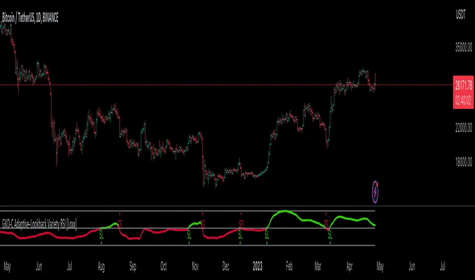
GKD-C Adaptive-Lookback Phase Change Index [Loxx]Giga Kaleidoscope GKD-C Adaptive-Lookback Phase Change Index is a Confirmation module included in Loxx's "Giga Kaleidoscope Modularized Trading System".
█ GKD-C Adaptive-Lookback Phase Change Index
What is the Phase Change Index?
The Phase Change Index (PCI) is a technical indicator that has gained popularity among traders in recent years. It is used to identify market phases and make profitable trades based on momentum and price data. The PCI was developed by M.H. Pee and first introduced in the Stocks & Commodities magazine in 2004.
The PCI is calculated using the 35-day momentum and the 35-day price channel index (PCI). The momentum is the difference between the current day's close and the close 35 days ago, while the PCI measures the distance between the highest high and lowest low over a period of 35 days. By combining these two indicators, traders can identify six possible market phases, each with its own trading strategy.
The formula for calculating the Phase Change Index (PCI) is as follows:
PCI = 100 * (C - L) / (H - L)
Where:
- C is the closing price of the current day
- L is the lowest low over a period of 35 days
- H is the highest high over a period of 35 days
The formula for calculating momentum is as follows:
Momentum = C - Cn
Where:
- C is the closing price of the current day
- Cn is the closing price n days ago, where n = 35 in this case.
The first two phases are characterized by negative momentum, with phase one having a low PCI value (less than 20) and phase two having a high PCI value (greater than 80). In these phases, traders should enter short positions. The next two phases have positive momentum, with phase three having a low PCI value and phase four having a high PCI value. In these phases, traders should enter long positions.
The final two phases are characterized by neutral momentum, with phase five having a low PCI value and phase six having a high PCI value. In these phases, traders should maintain their previous positions until there is a clear signal to enter or exit.
Traders can also use other technical indicators in conjunction with the PCI to confirm signals or filter out false signals. For example, some traders use moving averages or trendlines to confirm trend direction before entering a trade based on the PCI.
In conclusion, the Phase Change Index is a powerful technical indicator that can help traders identify market phases and make profitable trades. By combining momentum and price data, traders can enter long or short positions based on the six possible market phases. Backtesting results have shown that the PCI is robust across parameters, markets, and years. However, it is important to use proper risk management and not rely solely on past profitability when making trading decisions.
What is the Jurik Filter?
The Jurik Filter is a technical analysis tool that is used to filter out market noise and identify trends in financial markets. It was developed by Mark Jurik in the 1990s and is based on a non-linear smoothing algorithm that provides a more accurate representation of price movements.
Traditional moving averages, such as the Simple Moving Average ( SMA ) or Exponential Moving Average ( EMA ), are linear filters that produce a lag between price and the moving average line. This can cause false signals during periods of market volatility , which can result in losses for traders and investors.
The Jurik Filter is designed to address this issue by incorporating a damping factor into the smoothing algorithm. This damping factor adjusts the filter's responsiveness to the changes in price, allowing it to filter out market noise without overshooting price peaks and valleys.
The Jurik Filter is calculated using a mathematical formula that takes into account the current and past prices of an asset, as well as the volatility of the market. This formula incorporates the damping factor and produces a smoother price curve than traditional moving average filters.
One of the advantages of the Jurik Filter is its ability to adjust to changing market conditions. The damping factor can be adjusted to suit different securities and time frames, making it a versatile tool for traders and investors.
Traders and investors often use the Jurik Filter in conjunction with other technical analysis tools, such as the MACD or RSI , to confirm or complement their trading strategies. By filtering out market noise and identifying trends in the financial markets, the Jurik Filter can help improve the accuracy of trading signals and reduce the risks of false signals during periods of market volatility .
Overall, the Jurik Filter is a powerful technical analysis tool that can help traders and investors make more informed decisions about buying and selling securities. By providing a smoother price curve and reducing false signals, it can help improve trading performance and reduce risk in volatile markets.
What is the Adaptive Lookback Period?
The adaptive lookback period is a technique used in technical analysis to adjust the period of an indicator based on changes in market conditions. This technique is particularly useful in volatile or rapidly changing markets where a fixed period may not be optimal for detecting trends or signals.
The concept of the adaptive lookback period is relatively simple. By adjusting the lookback period based on changes in market conditions, traders can more accurately identify trends and signals. This can help traders to enter and exit trades at the right time and improve the profitability of their trading strategies.
The adaptive lookback period works by identifying potential swing points in the market. Once these points are identified, the lookback period is calculated based on the number of swings and a speed parameter. The swing count parameter determines the number of swings that must occur before the lookback period is adjusted. The speed parameter controls the rate at which the lookback period is adjusted, with higher values indicating a more rapid adjustment.
The adaptive lookback period can be applied to a wide range of technical indicators, including moving averages, oscillators, and trendlines. By adjusting the period of these indicators based on changes in market conditions, traders can reduce the impact of noise and false signals, leading to more profitable trades.
In summary, the adaptive lookback period is a powerful technique for traders and analysts looking to optimize their technical indicators. By adjusting the period based on changes in market conditions, traders can more accurately identify trends and signals, leading to more profitable trades. While there are various ways to implement the adaptive lookback period, the basic concept remains the same, and traders can adapt and customize the technique to suit their individual needs and trading styles.
What is the Adaptive-Lookback Phase Change Index?
The combination of adaptive lookback and Jurik filtering is an effective technique used in technical analysis to filter out market noise and improve the accuracy of trading signals. When applied to the Phase Change Index (PCI) indicator, the adaptive lookback period can be used to adjust the period of the indicator based on changes in market conditions. Jurik filtering can then be used to filter out market noise and improve the accuracy of the signals produced by the PCI indicator.
The adaptive lookback period is particularly useful in volatile or rapidly changing markets where a fixed period may not be optimal for detecting trends or signals. By adjusting the lookback period based on changes in market conditions, traders can more accurately identify trends and signals, leading to more profitable trades.
Jurik filtering is a more advanced filtering technique that uses a combination of smoothing and phase shift to produce a more accurate signal. This technique is particularly useful in filtering out market noise and improving the accuracy of trading signals. Jurik filtering can be applied to various indicators, including moving averages, oscillators, and trendlines.
Overall, the combination of adaptive lookback and Jurik filtering is a powerful technique used in technical analysis to filter out market noise and improve the accuracy of trading signals. When applied to the Phase Change Index (PCI) indicator, this technique is particularly effective in identifying trend changes and producing more accurate signals for entry and exit points in trading strategies.
Keep in mind, this is an inverse indicator meaning that above the middle-line/signal is short, below is long.
Additional Features
This indicator allows you to select from 33 source types. They are as follows:
Close
Open
High
Low
Median
Typical
Weighted
Average
Average Median Body
Trend Biased
Trend Biased (Extreme)
HA Close
HA Open
HA High
HA Low
HA Median
HA Typical
HA Weighted
HA Average
HA Average Median Body
HA Trend Biased
HA Trend Biased (Extreme)
HAB Close
HAB Open
HAB High
HAB Low
HAB Median
HAB Typical
HAB Weighted
HAB Average
HAB Average Median Body
HAB Trend Biased
HAB Trend Biased (Extreme)
What are Heiken Ashi "better" candles?
Heiken Ashi "better" candles are a modified version of the standard Heiken Ashi candles, which are a popular charting technique used in technical analysis. Heiken Ashi candles help traders identify trends and potential reversal points by smoothing out price data and reducing market noise. The "better formula" was proposed by Sebastian Schmidt in an article published by BNP Paribas in Warrants & Zertifikate, a German magazine, in August 2004. The aim of this formula is to further improve the smoothing of the Heiken Ashi chart and enhance its effectiveness in identifying trends and reversals.
Standard Heiken Ashi candles are calculated using the following formulas:
Heiken Ashi Close = (Open + High + Low + Close) / 4
Heiken Ashi Open = (Previous Heiken Ashi Open + Previous Heiken Ashi Close) / 2
Heiken Ashi High = Max (High, Heiken Ashi Open, Heiken Ashi Close)
Heiken Ashi Low = Min (Low, Heiken Ashi Open, Heiken Ashi Close)
The "better formula" modifies the standard Heiken Ashi calculation by incorporating additional smoothing, which can help reduce noise and make it easier to identify trends and reversals. The modified formulas for Heiken Ashi "better" candles are as follows:
Better Heiken Ashi Close = (Open + High + Low + Close) / 4
Better Heiken Ashi Open = (Previous Better Heiken Ashi Open + Previous Better Heiken Ashi Close) / 2
Better Heiken Ashi High = Max (High, Better Heiken Ashi Open, Better Heiken Ashi Close)
Better Heiken Ashi Low = Min (Low, Better Heiken Ashi Open, Better Heiken Ashi Close)
Smoothing Factor = 2 / (N + 1), where N is the chosen period for smoothing
Smoothed Better Heiken Ashi Open = (Better Heiken Ashi Open * Smoothing Factor) + (Previous Smoothed Better Heiken Ashi Open * (1 - Smoothing Factor))
Smoothed Better Heiken Ashi Close = (Better Heiken Ashi Close * Smoothing Factor) + (Previous Smoothed Better Heiken Ashi Close * (1 - Smoothing Factor))
The smoothed Better Heiken Ashi Open and Close values are then used to calculate the smoothed Better Heiken Ashi High and Low values, resulting in "better" candles that provide a clearer representation of the market trend and potential reversal points.
It's important to note that, like any other technical analysis tool, Heiken Ashi "better" candles are not foolproof and should be used in conjunction with other indicators and analysis techniques to make well-informed trading decisions.
Heiken Ashi "better" candles, as mentioned previously, provide a clearer representation of market trends and potential reversal points by reducing noise and smoothing out price data. When using these candles in conjunction with other technical analysis tools and indicators, traders can gain valuable insights into market behavior and make more informed decisions.
To effectively use Heiken Ashi "better" candles in your trading strategy, consider the following tips:
Trend Identification: Heiken Ashi "better" candles can help you identify the prevailing trend in the market. When the majority of the candles are green (or another color, depending on your chart settings) and there are no or few lower wicks, it may indicate a strong uptrend. Conversely, when the majority of the candles are red (or another color) and there are no or few upper wicks, it may signal a strong downtrend.
Trend Reversals: Look for potential trend reversals when a change in the color of the candles occurs, especially when accompanied by longer wicks. For example, if a green candle with a long lower wick is followed by a red candle, it could indicate a bearish reversal. Similarly, a red candle with a long upper wick followed by a green candle may suggest a bullish reversal.
Support and Resistance: You can use Heiken Ashi "better" candles to identify potential support and resistance levels. When the candles are consistently moving in one direction and then suddenly change color with longer wicks, it could indicate the presence of a support or resistance level.
Stop-Loss and Take-Profit: Using Heiken Ashi "better" candles can help you manage risk by determining optimal stop-loss and take-profit levels. For instance, you can place your stop-loss below the low of the most recent green candle in an uptrend or above the high of the most recent red candle in a downtrend.
Confirming Signals: Heiken Ashi "better" candles should be used in conjunction with other technical indicators, such as moving averages, oscillators, or chart patterns, to confirm signals and improve the accuracy of your analysis.
In this implementation, you have the choice of AMA, KAMA, or T3 smoothing. These are as follows:
Kaufman Adaptive Moving Average (KAMA)
The Kaufman Adaptive Moving Average (KAMA) is a type of adaptive moving average used in technical analysis to smooth out price fluctuations and identify trends. The KAMA adjusts its smoothing factor based on the market's volatility, making it more responsive in volatile markets and smoother in calm markets. The KAMA is calculated using three different efficiency ratios that determine the appropriate smoothing factor for the current market conditions. These ratios are based on the noise level of the market, the speed at which the market is moving, and the length of the moving average. The KAMA is a popular choice among traders who prefer to use adaptive indicators to identify trends and potential reversals.
Adaptive Moving Average
The Adaptive Moving Average (AMA) is a type of moving average that adjusts its sensitivity to price movements based on market conditions. It uses a ratio between the current price and the highest and lowest prices over a certain lookback period to determine its level of smoothing. The AMA can help reduce lag and increase responsiveness to changes in trend direction, making it useful for traders who want to follow trends while avoiding false signals. The AMA is calculated by multiplying a smoothing constant with the difference between the current price and the previous AMA value, then adding the result to the previous AMA value.
T3
The T3 moving average is a type of technical indicator used in financial analysis to identify trends in price movements. It is similar to the Exponential Moving Average (EMA) and the Double Exponential Moving Average (DEMA), but uses a different smoothing algorithm.
The T3 moving average is calculated using a series of exponential moving averages that are designed to filter out noise and smooth the data. The resulting smoothed data is then weighted with a non-linear function to produce a final output that is more responsive to changes in trend direction.
The T3 moving average can be customized by adjusting the length of the moving average, as well as the weighting function used to smooth the data. It is commonly used in conjunction with other technical indicators as part of a larger trading strategy.
█ Giga Kaleidoscope Modularized Trading System
Core components of an NNFX algorithmic trading strategy
The NNFX algorithm is built on the principles of trend, momentum, and volatility. There are six core components in the NNFX trading algorithm:
1. Volatility - price volatility; e.g., Average True Range, True Range Double, Close-to-Close, etc.
2. Baseline - a moving average to identify price trend
3. Confirmation 1 - a technical indicator used to identify trends
4. Confirmation 2 - a technical indicator used to identify trends
5. Continuation - a technical indicator used to identify trends
6. Volatility/Volume - a technical indicator used to identify volatility/volume breakouts/breakdown
7. Exit - a technical indicator used to determine when a trend is exhausted
What is Volatility in the NNFX trading system?
In the NNFX (No Nonsense Forex) trading system, ATR (Average True Range) is typically used to measure the volatility of an asset. It is used as a part of the system to help determine the appropriate stop loss and take profit levels for a trade. ATR is calculated by taking the average of the true range values over a specified period.
True range is calculated as the maximum of the following values:
-Current high minus the current low
-Absolute value of the current high minus the previous close
-Absolute value of the current low minus the previous close
ATR is a dynamic indicator that changes with changes in volatility. As volatility increases, the value of ATR increases, and as volatility decreases, the value of ATR decreases. By using ATR in NNFX system, traders can adjust their stop loss and take profit levels according to the volatility of the asset being traded. This helps to ensure that the trade is given enough room to move, while also minimizing potential losses.
Other types of volatility include True Range Double (TRD), Close-to-Close, and Garman-Klass
What is a Baseline indicator?
The baseline is essentially a moving average, and is used to determine the overall direction of the market.
The baseline in the NNFX system is used to filter out trades that are not in line with the long-term trend of the market. The baseline is plotted on the chart along with other indicators, such as the Moving Average (MA), the Relative Strength Index (RSI), and the Average True Range (ATR).
Trades are only taken when the price is in the same direction as the baseline. For example, if the baseline is sloping upwards, only long trades are taken, and if the baseline is sloping downwards, only short trades are taken. This approach helps to ensure that trades are in line with the overall trend of the market, and reduces the risk of entering trades that are likely to fail.
By using a baseline in the NNFX system, traders can have a clear reference point for determining the overall trend of the market, and can make more informed trading decisions. The baseline helps to filter out noise and false signals, and ensures that trades are taken in the direction of the long-term trend.
What is a Confirmation indicator?
Confirmation indicators are technical indicators that are used to confirm the signals generated by primary indicators. Primary indicators are the core indicators used in the NNFX system, such as the Average True Range (ATR), the Moving Average (MA), and the Relative Strength Index (RSI).
The purpose of the confirmation indicators is to reduce false signals and improve the accuracy of the trading system. They are designed to confirm the signals generated by the primary indicators by providing additional information about the strength and direction of the trend.
Some examples of confirmation indicators that may be used in the NNFX system include the Bollinger Bands, the MACD (Moving Average Convergence Divergence), and the MACD Oscillator. These indicators can provide information about the volatility, momentum, and trend strength of the market, and can be used to confirm the signals generated by the primary indicators.
In the NNFX system, confirmation indicators are used in combination with primary indicators and other filters to create a trading system that is robust and reliable. By using multiple indicators to confirm trading signals, the system aims to reduce the risk of false signals and improve the overall profitability of the trades.
What is a Continuation indicator?
In the NNFX (No Nonsense Forex) trading system, a continuation indicator is a technical indicator that is used to confirm a current trend and predict that the trend is likely to continue in the same direction. A continuation indicator is typically used in conjunction with other indicators in the system, such as a baseline indicator, to provide a comprehensive trading strategy.
What is a Volatility/Volume indicator?
Volume indicators, such as the On Balance Volume (OBV), the Chaikin Money Flow (CMF), or the Volume Price Trend (VPT), are used to measure the amount of buying and selling activity in a market. They are based on the trading volume of the market, and can provide information about the strength of the trend. In the NNFX system, volume indicators are used to confirm trading signals generated by the Moving Average and the Relative Strength Index. Volatility indicators include Average Direction Index, Waddah Attar, and Volatility Ratio. In the NNFX trading system, volatility is a proxy for volume and vice versa.
By using volume indicators as confirmation tools, the NNFX trading system aims to reduce the risk of false signals and improve the overall profitability of trades. These indicators can provide additional information about the market that is not captured by the primary indicators, and can help traders to make more informed trading decisions. In addition, volume indicators can be used to identify potential changes in market trends and to confirm the strength of price movements.
What is an Exit indicator?
The exit indicator is used in conjunction with other indicators in the system, such as the Moving Average (MA), the Relative Strength Index (RSI), and the Average True Range (ATR), to provide a comprehensive trading strategy.
The exit indicator in the NNFX system can be any technical indicator that is deemed effective at identifying optimal exit points. Examples of exit indicators that are commonly used include the Parabolic SAR, the Average Directional Index (ADX), and the Chandelier Exit.
The purpose of the exit indicator is to identify when a trend is likely to reverse or when the market conditions have changed, signaling the need to exit a trade. By using an exit indicator, traders can manage their risk and prevent significant losses.
In the NNFX system, the exit indicator is used in conjunction with a stop loss and a take profit order to maximize profits and minimize losses. The stop loss order is used to limit the amount of loss that can be incurred if the trade goes against the trader, while the take profit order is used to lock in profits when the trade is moving in the trader's favor.
Overall, the use of an exit indicator in the NNFX trading system is an important component of a comprehensive trading strategy. It allows traders to manage their risk effectively and improve the profitability of their trades by exiting at the right time.
How does Loxx's GKD (Giga Kaleidoscope Modularized Trading System) implement the NNFX algorithm outlined above?
Loxx's GKD v1.0 system has five types of modules (indicators/strategies). These modules are:
1. GKD-BT - Backtesting module (Volatility, Number 1 in the NNFX algorithm)
2. GKD-B - Baseline module (Baseline and Volatility/Volume, Numbers 1 and 2 in the NNFX algorithm)
3. GKD-C - Confirmation 1/2 and Continuation module (Confirmation 1/2 and Continuation, Numbers 3, 4, and 5 in the NNFX algorithm)
4. GKD-V - Volatility/Volume module (Confirmation 1/2, Number 6 in the NNFX algorithm)
5. GKD-E - Exit module (Exit, Number 7 in the NNFX algorithm)
(additional module types will added in future releases)
Each module interacts with every module by passing data between modules. Data is passed between each module as described below:
GKD-B => GKD-V => GKD-C(1) => GKD-C(2) => GKD-C(Continuation) => GKD-E => GKD-BT
That is, the Baseline indicator passes its data to Volatility/Volume. The Volatility/Volume indicator passes its values to the Confirmation 1 indicator. The Confirmation 1 indicator passes its values to the Confirmation 2 indicator. The Confirmation 2 indicator passes its values to the Continuation indicator. The Continuation indicator passes its values to the Exit indicator, and finally, the Exit indicator passes its values to the Backtest strategy.
This chaining of indicators requires that each module conform to Loxx's GKD protocol, therefore allowing for the testing of every possible combination of technical indicators that make up the six components of the NNFX algorithm.
What does the application of the GKD trading system look like?
Example trading system:
Backtest: Strategy with 1-3 take profits, trailing stop loss, multiple types of PnL volatility, and 2 backtesting styles
Baseline: Hull Moving Average
Volatility/Volume: Hurst Exponent
Confirmation 1: Adaptive-Lookback Phase Change Index as shown on the chart above
Confirmation 2: Williams Percent Range
Continuation: Fisher Transform
Exit: Rex Oscillator
Each GKD indicator is denoted with a module identifier of either: GKD-BT, GKD-B, GKD-C, GKD-V, or GKD-E. This allows traders to understand to which module each indicator belongs and where each indicator fits into the GKD protocol chain.
Giga Kaleidoscope Modularized Trading System Signals (based on the NNFX algorithm)
Standard Entry
1. GKD-C Confirmation 1 Signal
2. GKD-B Baseline agrees
3. Price is within a range of 0.2x Volatility and 1.0x Volatility of the Goldie Locks Mean
4. GKD-C Confirmation 2 agrees
5. GKD-V Volatility/Volume agrees
Baseline Entry
1. GKD-B Baseline signal
2. GKD-C Confirmation 1 agrees
3. Price is within a range of 0.2x Volatility and 1.0x Volatility of the Goldie Locks Mean
4. GKD-C Confirmation 2 agrees
5. GKD-V Volatility/Volume agrees
6. GKD-C Confirmation 1 signal was less than 7 candles prior
Volatility/Volume Entry
1. GKD-V Volatility/Volume signal
2. GKD-C Confirmation 1 agrees
3. Price is within a range of 0.2x Volatility and 1.0x Volatility of the Goldie Locks Mean
4. GKD-C Confirmation 2 agrees
5. GKD-B Baseline agrees
6. GKD-C Confirmation 1 signal was less than 7 candles prior
Continuation Entry
1. Standard Entry, Baseline Entry, or Pullback; entry triggered previously
2. GKD-B Baseline hasn't crossed since entry signal trigger
3. GKD-C Confirmation Continuation Indicator signals
4. GKD-C Confirmation 1 agrees
5. GKD-B Baseline agrees
6. GKD-C Confirmation 2 agrees
1-Candle Rule Standard Entry
1. GKD-C Confirmation 1 signal
2. GKD-B Baseline agrees
3. Price is within a range of 0.2x Volatility and 1.0x Volatility of the Goldie Locks Mean
Next Candle:
1. Price retraced (Long: close < close or Short: close > close )
2. GKD-B Baseline agrees
3. GKD-C Confirmation 1 agrees
4. GKD-C Confirmation 2 agrees
5. GKD-V Volatility/Volume agrees
1-Candle Rule Baseline Entry
1. GKD-B Baseline signal
2. GKD-C Confirmation 1 agrees
3. Price is within a range of 0.2x Volatility and 1.0x Volatility of the Goldie Locks Mean
4. GKD-C Confirmation 1 signal was less than 7 candles prior
Next Candle:
1. Price retraced (Long: close < close or Short: close > close )
2. GKD-B Baseline agrees
3. GKD-C Confirmation 1 agrees
4. GKD-C Confirmation 2 agrees
5. GKD-V Volatility/Volume Agrees
1-Candle Rule Volatility/Volume Entry
1. GKD-V Volatility/Volume signal
2. GKD-C Confirmation 1 agrees
3. Price is within a range of 0.2x Volatility and 1.0x Volatility of the Goldie Locks Mean
4. GKD-C Confirmation 1 signal was less than 7 candles prior
Next Candle:
1. Price retraced (Long: close < close or Short: close > close)
2. GKD-B Volatility/Volume agrees
3. GKD-C Confirmation 1 agrees
4. GKD-C Confirmation 2 agrees
5. GKD-B Baseline agrees
PullBack Entry
1. GKD-B Baseline signal
2. GKD-C Confirmation 1 agrees
3. Price is beyond 1.0x Volatility of Baseline
Next Candle:
1. Price is within a range of 0.2x Volatility and 1.0x Volatility of the Goldie Locks Mean
2. GKD-C Confirmation 1 agrees
3. GKD-C Confirmation 2 agrees
4. GKD-V Volatility/Volume Agrees
]█ Setting up the GKD
The GKD system involves chaining indicators together. These are the steps to set this up.
Use a GKD-C indicator alone on a chart
1. Inside the GKD-C indicator, change the "Confirmation Type" setting to "Solo Confirmation Simple"
Use a GKD-V indicator alone on a chart
**nothing, it's already useable on the chart without any settings changes
Use a GKD-B indicator alone on a chart
**nothing, it's already useable on the chart without any settings changes
Baseline (Baseline, Backtest)
1. Import the GKD-B Baseline into the GKD-BT Backtest: "Input into Volatility/Volume or Backtest (Baseline testing)"
2. Inside the GKD-BT Backtest, change the setting "Backtest Special" to "Baseline"
Volatility/Volume (Volatility/Volume, Backte st)
1. Inside the GKD-V indicator, change the "Testing Type" setting to "Solo"
2. Inside the GKD-V indicator, change the "Signal Type" setting to "Crossing" (neither traditional nor both can be backtested)
3. Import the GKD-V indicator into the GKD-BT Backtest: "Input into C1 or Backtest"
4. Inside the GKD-BT Backtest, change the setting "Backtest Special" to "Volatility/Volume"
5. Inside the GKD-BT Backtest, a) change the setting "Backtest Type" to "Trading" if using a directional GKD-V indicator; or, b) change the setting "Backtest Type" to "Full" if using a directional or non-directional GKD-V indicator (non-directional GKD-V can only test Longs and Shorts separately)
6. If "Backtest Type" is set to "Full": Inside the GKD-BT Backtest, change the setting "Backtest Side" to "Long" or "Short
7. If "Backtest Type" is set to "Full": To allow the system to open multiple orders at one time so you test all Longs or Shorts, open the GKD-BT Backtest, click the tab "Properties" and then insert a value of something like 10 orders into the "Pyramiding" settings. This will allow 10 orders to be opened at one time which should be enough to catch all possible Longs or Shorts.
Solo Confirmation Simple (Confirmation, Backtest)
1. Inside the GKD-C indicator, change the "Confirmation Type" setting to "Solo Confirmation Simple"
1. Import the GKD-C indicator into the GKD-BT Backtest: "Input into Backtest"
2. Inside the GKD-BT Backtest, change the setting "Backtest Special" to "Solo Confirmation Simple"
Solo Confirmation Complex without Exits (Baseline, Volatility/Volume, Confirmation, Backtest)
1. Inside the GKD-V indicator, change the "Testing Type" setting to "Chained"
2. Import the GKD-B Baseline into the GKD-V indicator: "Input into Volatility/Volume or Backtest (Baseline testing)"
3. Inside the GKD-C indicator, change the "Confirmation Type" setting to "Solo Confirmation Complex"
4. Import the GKD-V indicator into the GKD-C indicator: "Input into C1 or Backtest"
5. Inside the GKD-BT Backtest, change the setting "Backtest Special" to "GKD Full wo/ Exits"
6. Import the GKD-C into the GKD-BT Backtest: "Input into Exit or Backtest"
Solo Confirmation Complex with Exits (Baseline, Volatility/Volume, Confirmation, Exit, Backtest)
1. Inside the GKD-V indicator, change the "Testing Type" setting to "Chained"
2. Import the GKD-B Baseline into the GKD-V indicator: "Input into Volatility/Volume or Backtest (Baseline testing)"
3. Inside the GKD-C indicator, change the "Confirmation Type" setting to "Solo Confirmation Complex"
4. Import the GKD-V indicator into the GKD-C indicator: "Input into C1 or Backtest"
5. Import the GKD-C indicator into the GKD-E indicator: "Input into Exit"
6. Inside the GKD-BT Backtest, change the setting "Backtest Special" to "GKD Full w/ Exits"
7. Import the GKD-E into the GKD-BT Backtest: "Input into Backtest"
Full GKD without Exits (Baseline, Volatility/Volume, Confirmation 1, Confirmation 2, Continuation, Backtest)
1. Inside the GKD-V indicator, change the "Testing Type" setting to "Chained"
2. Import the GKD-B Baseline into the GKD-V indicator: "Input into Volatility/Volume or Backtest (Baseline testing)"
3. Inside the GKD-C 1 indicator, change the "Confirmation Type" setting to "Confirmation 1"
4. Import the GKD-V indicator into the GKD-C 1 indicator: "Input into C1 or Backtest"
5. Inside the GKD-C 2 indicator, change the "Confirmation Type" setting to "Confirmation 2"
6. Import the GKD-C 1 indicator into the GKD-C 2 indicator: "Input into C2"
7. Inside the GKD-C Continuation indicator, change the "Confirmation Type" setting to "Continuation"
8. Inside the GKD-BT Backtest, change the setting "Backtest Special" to "GKD Full wo/ Exits"
9. Import the GKD-E into the GKD-BT Backtest: "Input into Exit or Backtest"
Full GKD with Exits (Baseline, Volatility/Volume, Confirmation 1, Confirmation 2, Continuation, Exit, Backtest)
1. Inside the GKD-V indicator, change the "Testing Type" setting to "Chained"
2. Import the GKD-B Baseline into the GKD-V indicator: "Input into Volatility/Volume or Backtest (Baseline testing)"
3. Inside the GKD-C 1 indicator, change the "Confirmation Type" setting to "Confirmation 1"
4. Import the GKD-V indicator into the GKD-C 1 indicator: "Input into C1 or Backtest"
5. Inside the GKD-C 2 indicator, change the "Confirmation Type" setting to "Confirmation 2"
6. Import the GKD-C 1 indicator into the GKD-C 2 indicator: "Input into C2"
7. Inside the GKD-C Continuation indicator, change the "Confirmation Type" setting to "Continuation"
8. Import the GKD-C Continuation indicator into the GKD-E indicator: "Input into Exit"
9. Inside the GKD-BT Backtest, change the setting "Backtest Special" to "GKD Full w/ Exits"
10. Import the GKD-E into the GKD-BT Backtest: "Input into Backtest"
Baseline + Volatility/Volume (Baseline, Volatility/Volume, Backtest)
1. Inside the GKD-V indicator, change the "Testing Type" setting to "Baseline + Volatility/Volume"
2. Inside the GKD-V indicator, make sure the "Signal Type" setting is set to "Traditional"
3. Import the GKD-B Baseline into the GKD-V indicator: "Input into Volatility/Volume or Backtest (Baseline testing)"
4. Inside the GKD-BT Backtest, change the setting "Backtest Special" to "Baseline + Volatility/Volume"
5. Import the GKD-V into the GKD-BT Backtest: "Input into C1 or Backtest"
6. Inside the GKD-BT Backtest, change the setting "Backtest Type" to "Full". For this backtest, you must test Longs and Shorts separately
7. To allow the system to open multiple orders at one time so you can test all Longs or Shorts, open the GKD-BT Backtest, click the tab "Properties" and then insert a value of something like 10 orders into the "Pyramiding" settings. This will allow 10 orders to be opened at one time which should be enough to catch all possible Longs or Shorts.
Requirements
Inputs
Confirmation 1: GKD-V Volatility / Volume indicator
Confirmation 2: GKD-C Confirmation indicator
Continuation: GKD-C Confirmation indicator
Solo Confirmation Simple: GKD-B Baseline
Solo Confirmation Complex: GKD-V Volatility / Volume indicator
Solo Confirmation Super Complex: GKD-V Volatility / Volume indicator
Stacked 1: None
Stacked 2+: GKD-C, GKD-V, or GKD-B Stacked 1
Outputs
Confirmation 1: GKD-C Confirmation 2 indicator
Confirmation 2: GKD-C Continuation indicator
Continuation: GKD-E Exit indicator
Solo Confirmation Simple: GKD-BT Backtest
Solo Confirmation Complex: GKD-BT Backtest or GKD-E Exit indicator
Solo Confirmation Super Complex: GKD-C Continuation indicator
Stacked 1: GKD-C, GKD-V, or GKD-B Stacked 2+
Stacked 2+: GKD-C, GKD-V, or GKD-B Stacked 2+ or GKD-BT Backtest
Additional features will be added in future releases.
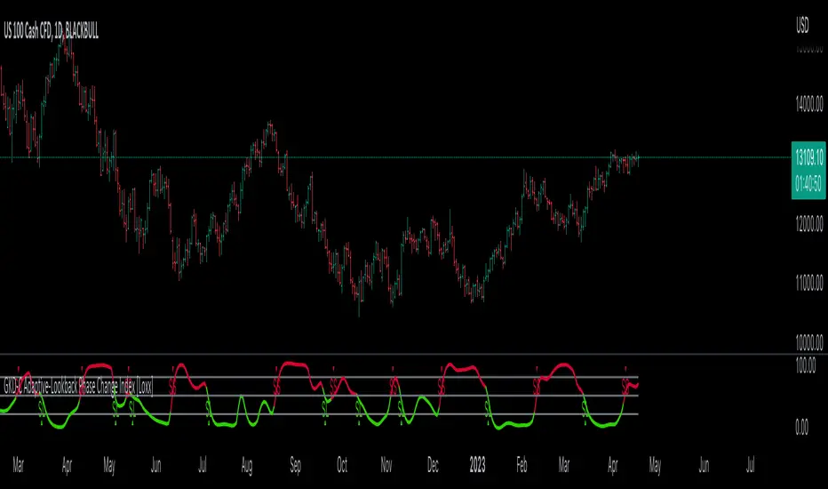
GKD-C Adaptive Digital Kahler Variety RSI w/ DZ [Loxx]Giga Kaleidoscope GKD-C Adaptive Digital Kahler Variety RSI w/ DZ is a Confirmation module included in Loxx's "Giga Kaleidoscope Modularized Trading System".
█ Giga Kaleidoscope Modularized Trading System
What is Loxx's "Giga Kaleidoscope Modularized Trading System"?
The Giga Kaleidoscope Modularized Trading System is a trading system built on the philosophy of the NNFX (No Nonsense Forex) algorithmic trading.
What is the NNFX algorithmic trading strategy?
The NNFX (No-Nonsense Forex) trading system is a comprehensive approach to Forex trading that is designed to simplify the process and remove the confusion and complexity that often surrounds trading. The system was developed by a Forex trader who goes by the pseudonym "VP" and has gained a significant following in the Forex community.
The NNFX trading system is based on a set of rules and guidelines that help traders make objective and informed decisions. These rules cover all aspects of trading, including market analysis, trade entry, stop loss placement, and trade management.
Here are the main components of the NNFX trading system:
1. Trading Philosophy: The NNFX trading system is based on the idea that successful trading requires a comprehensive understanding of the market, objective analysis, and strict risk management. The system aims to remove subjective elements from trading and focuses on objective rules and guidelines.
2. Technical Analysis: The NNFX trading system relies heavily on technical analysis and uses a range of indicators to identify high-probability trading opportunities. The system uses a combination of trend-following and mean-reverting strategies to identify trades.
3. Market Structure: The NNFX trading system emphasizes the importance of understanding the market structure, including price action, support and resistance levels, and market cycles. The system uses a range of tools to identify the market structure, including trend lines, channels, and moving averages.
4. Trade Entry: The NNFX trading system has strict rules for trade entry. The system uses a combination of technical indicators to identify high-probability trades, and traders must meet specific criteria to enter a trade.
5. Stop Loss Placement: The NNFX trading system places a significant emphasis on risk management and requires traders to place a stop loss order on every trade. The system uses a combination of technical analysis and market structure to determine the appropriate stop loss level.
6. Trade Management: The NNFX trading system has specific rules for managing open trades. The system aims to minimize risk and maximize profit by using a combination of trailing stops, take profit levels, and position sizing.
Overall, the NNFX trading system is designed to be a straightforward and easy-to-follow approach to Forex trading that can be applied by traders of all skill levels.
Core components of an NNFX algorithmic trading strategy
The NNFX algorithm is built on the principles of trend, momentum, and volatility. There are six core components in the NNFX trading algorithm:
1. Volatility - price volatility; e.g., Average True Range, True Range Double, Close-to-Close, etc.
2. Baseline - a moving average to identify price trend
3. Confirmation 1 - a technical indicator used to identify trends
4. Confirmation 2 - a technical indicator used to identify trends
5. Continuation - a technical indicator used to identify trends
6. Volatility/Volume - a technical indicator used to identify volatility/volume breakouts/breakdown
7. Exit - a technical indicator used to determine when a trend is exhausted
What is Volatility in the NNFX trading system?
In the NNFX (No Nonsense Forex) trading system, ATR (Average True Range) is typically used to measure the volatility of an asset. It is used as a part of the system to help determine the appropriate stop loss and take profit levels for a trade. ATR is calculated by taking the average of the true range values over a specified period.
True range is calculated as the maximum of the following values:
-Current high minus the current low
-Absolute value of the current high minus the previous close
-Absolute value of the current low minus the previous close
ATR is a dynamic indicator that changes with changes in volatility. As volatility increases, the value of ATR increases, and as volatility decreases, the value of ATR decreases. By using ATR in NNFX system, traders can adjust their stop loss and take profit levels according to the volatility of the asset being traded. This helps to ensure that the trade is given enough room to move, while also minimizing potential losses.
Other types of volatility include True Range Double (TRD), Close-to-Close, and Garman-Klass
What is a Baseline indicator?
The baseline is essentially a moving average, and is used to determine the overall direction of the market.
The baseline in the NNFX system is used to filter out trades that are not in line with the long-term trend of the market. The baseline is plotted on the chart along with other indicators, such as the Moving Average (MA), the Relative Strength Index (RSI), and the Average True Range (ATR).
Trades are only taken when the price is in the same direction as the baseline. For example, if the baseline is sloping upwards, only long trades are taken, and if the baseline is sloping downwards, only short trades are taken. This approach helps to ensure that trades are in line with the overall trend of the market, and reduces the risk of entering trades that are likely to fail.
By using a baseline in the NNFX system, traders can have a clear reference point for determining the overall trend of the market, and can make more informed trading decisions. The baseline helps to filter out noise and false signals, and ensures that trades are taken in the direction of the long-term trend.
What is a Confirmation indicator?
Confirmation indicators are technical indicators that are used to confirm the signals generated by primary indicators. Primary indicators are the core indicators used in the NNFX system, such as the Average True Range (ATR), the Moving Average (MA), and the Relative Strength Index (RSI).
The purpose of the confirmation indicators is to reduce false signals and improve the accuracy of the trading system. They are designed to confirm the signals generated by the primary indicators by providing additional information about the strength and direction of the trend.
Some examples of confirmation indicators that may be used in the NNFX system include the Bollinger Bands, the MACD (Moving Average Convergence Divergence), and the MACD Oscillator. These indicators can provide information about the volatility, momentum, and trend strength of the market, and can be used to confirm the signals generated by the primary indicators.
In the NNFX system, confirmation indicators are used in combination with primary indicators and other filters to create a trading system that is robust and reliable. By using multiple indicators to confirm trading signals, the system aims to reduce the risk of false signals and improve the overall profitability of the trades.
What is a Continuation indicator?
In the NNFX (No Nonsense Forex) trading system, a continuation indicator is a technical indicator that is used to confirm a current trend and predict that the trend is likely to continue in the same direction. A continuation indicator is typically used in conjunction with other indicators in the system, such as a baseline indicator, to provide a comprehensive trading strategy.
What is a Volatility/Volume indicator?
Volume indicators, such as the On Balance Volume (OBV), the Chaikin Money Flow (CMF), or the Volume Price Trend (VPT), are used to measure the amount of buying and selling activity in a market. They are based on the trading volume of the market, and can provide information about the strength of the trend. In the NNFX system, volume indicators are used to confirm trading signals generated by the Moving Average and the Relative Strength Index. Volatility indicators include Average Direction Index, Waddah Attar, and Volatility Ratio. In the NNFX trading system, volatility is a proxy for volume and vice versa.
By using volume indicators as confirmation tools, the NNFX trading system aims to reduce the risk of false signals and improve the overall profitability of trades. These indicators can provide additional information about the market that is not captured by the primary indicators, and can help traders to make more informed trading decisions. In addition, volume indicators can be used to identify potential changes in market trends and to confirm the strength of price movements.
What is an Exit indicator?
The exit indicator is used in conjunction with other indicators in the system, such as the Moving Average (MA), the Relative Strength Index (RSI), and the Average True Range (ATR), to provide a comprehensive trading strategy.
The exit indicator in the NNFX system can be any technical indicator that is deemed effective at identifying optimal exit points. Examples of exit indicators that are commonly used include the Parabolic SAR, the Average Directional Index (ADX), and the Chandelier Exit.
The purpose of the exit indicator is to identify when a trend is likely to reverse or when the market conditions have changed, signaling the need to exit a trade. By using an exit indicator, traders can manage their risk and prevent significant losses.
In the NNFX system, the exit indicator is used in conjunction with a stop loss and a take profit order to maximize profits and minimize losses. The stop loss order is used to limit the amount of loss that can be incurred if the trade goes against the trader, while the take profit order is used to lock in profits when the trade is moving in the trader's favor.
Overall, the use of an exit indicator in the NNFX trading system is an important component of a comprehensive trading strategy. It allows traders to manage their risk effectively and improve the profitability of their trades by exiting at the right time.
How does Loxx's GKD (Giga Kaleidoscope Modularized Trading System) implement the NNFX algorithm outlined above?
Loxx's GKD v1.0 system has five types of modules (indicators/strategies). These modules are:
1. GKD-BT - Backtesting module (Volatility, Number 1 in the NNFX algorithm)
2. GKD-B - Baseline module (Baseline and Volatility/Volume, Numbers 1 and 2 in the NNFX algorithm)
3. GKD-C - Confirmation 1/2 and Continuation module (Confirmation 1/2 and Continuation, Numbers 3, 4, and 5 in the NNFX algorithm)
4. GKD-V - Volatility/Volume module (Confirmation 1/2, Number 6 in the NNFX algorithm)
5. GKD-E - Exit module (Exit, Number 7 in the NNFX algorithm)
(additional module types will added in future releases)
Each module interacts with every module by passing data between modules. Data is passed between each module as described below:
GKD-B => GKD-V => GKD-C(1) => GKD-C(2) => GKD-C(Continuation) => GKD-E => GKD-BT
That is, the Baseline indicator passes its data to Volatility/Volume. The Volatility/Volume indicator passes its values to the Confirmation 1 indicator. The Confirmation 1 indicator passes its values to the Confirmation 2 indicator. The Confirmation 2 indicator passes its values to the Continuation indicator. The Continuation indicator passes its values to the Exit indicator, and finally, the Exit indicator passes its values to the Backtest strategy.
This chaining of indicators requires that each module conform to Loxx's GKD protocol, therefore allowing for the testing of every possible combination of technical indicators that make up the six components of the NNFX algorithm.
What does the application of the GKD trading system look like?
Example trading system:
Backtest: Strategy with 1-3 take profits, trailing stop loss, multiple types of PnL volatility, and 2 backtesting styles
Baseline: Hull Moving Average
Volatility/Volume: Hurst Exponent
Confirmation 1: Adaptive Digital Kahler Variety RSI w/ DZ as shown on the chart above
Confirmation 2: Williams Percent Range
Continuation: Fisher Transform
Exit: Rex Oscillator
Each GKD indicator is denoted with a module identifier of either: GKD-BT, GKD-B, GKD-C, GKD-V, or GKD-E. This allows traders to understand to which module each indicator belongs and where each indicator fits into the GKD protocol chain.
Giga Kaleidoscope Modularized Trading System Signals (based on the NNFX algorithm)
Standard Entry
1. GKD-C Confirmation 1 Signal
2. GKD-B Baseline agrees
3. Price is within a range of 0.2x Volatility and 1.0x Volatility of the Goldie Locks Mean
4. GKD-C Confirmation 2 agrees
5. GKD-V Volatility/Volume agrees
Baseline Entry
1. GKD-B Baseline signal
2. GKD-C Confirmation 1 agrees
3. Price is within a range of 0.2x Volatility and 1.0x Volatility of the Goldie Locks Mean
4. GKD-C Confirmation 2 agrees
5. GKD-V Volatility/Volume agrees
6. GKD-C Confirmation 1 signal was less than 7 candles prior
Continuation Entry
1. Standard Entry, Baseline Entry, or Pullback; entry triggered previously
2. GKD-B Baseline hasn't crossed since entry signal trigger
3. GKD-C Confirmation Continuation Indicator signals
4. GKD-C Confirmation 1 agrees
5. GKD-B Baseline agrees
6. GKD-C Confirmation 2 agrees
1-Candle Rule Standard Entry
1. GKD-C Confirmation 1 signal
2. GKD-B Baseline agrees
3. Price is within a range of 0.2x Volatility and 1.0x Volatility of the Goldie Locks Mean
Next Candle:
1. Price retraced (Long: close < close or Short: close > close )
2. GKD-B Baseline agrees
3. GKD-C Confirmation 1 agrees
4. GKD-C Confirmation 2 agrees
5. GKD-V Volatility/Volume agrees
1-Candle Rule Baseline Entry
1. GKD-B Baseline signal
2. GKD-C Confirmation 1 agrees
3. Price is within a range of 0.2x Volatility and 1.0x Volatility of the Goldie Locks Mean
4. GKD-C Confirmation 1 signal was less than 7 candles prior
Next Candle:
1. Price retraced (Long: close < close or Short: close > close )
2. GKD-B Baseline agrees
3. GKD-C Confirmation 1 agrees
4. GKD-C Confirmation 2 agrees
5. GKD-V Volatility/Volume Agrees
PullBack Entry
1. GKD-B Baseline signal
2. GKD-C Confirmation 1 agrees
3. Price is beyond 1.0x Volatility of Baseline
Next Candle:
1. Price is within a range of 0.2x Volatility and 1.0x Volatility of the Goldie Locks Mean
3. GKD-C Confirmation 1 agrees
4. GKD-C Confirmation 2 agrees
5. GKD-V Volatility/Volume Agrees
█ GKD-C Adaptive Digital Kahler Variety RSI w/ DZ
What is Digital Kahler?
From Philipp Kahler's article for www.traders-mag.com, August 2008. "A Classic Indicator in a New Suit: Digital Stochastic"
Digital Indicators
Whenever you study the development of trading systems in particular, you will be struck in an extremely unpleasant way by the seemingly unmotivated indentations and changes in direction of each indicator. An experienced trader can recognise many false signals of the indicator on the basis of his solid background; a stupid trading system usually falls into any trap offered by the unclear indicator course. This is what motivated me to improve even further this and other indicators with the help of a relatively simple procedure. The goal of this development is to be able to use this indicator in a trading system with as few additional conditions as possible. Discretionary traders will likewise be happy about this clear course, which is not nerve-racking and makes concentrating on the essential elements of trading possible.
How Is It Done?
The digital stochastic is a child of the original indicator. We owe a debt of gratitude to George Lane for his idea to design an indicator which describes the position of the current price within the high-low range of the historical price movement. My contribution to this indicator is the changed pattern which improves the quality of the signal without generating too long delays in giving signals. The trick used to generate this “digital” behavior of the indicator. It can be used with most oscillators like RSI or CCI.
First of all, the original is looked at. The indicator always moves between 0 and 100. The precise position of the indicator or its course relative to the trigger line are of no interest to me, I would just like to know whether the indicator is quoted below or above the value 50. This is tantamount to the question of whether the market is just trading above or below the middle of the high-low range of the past few days. If the market trades in the upper half of its high-low range, then the digital stochastic is given the value 1; if the original stochastic is below 50, then the value –1 is given. This leads to a sequence of 1/-1 values – the digital core of the new indicator. These values are subsequently smoothed by means of a short exponential moving average . This way minor false signals are eliminated and the indicator is given its typical form.
This indicator contains 7 different types of RSI:
RSX
Regular
Slow
Rapid
Harris
Cuttler
Ehlers Smoothed
What is RSI?
RSI stands for Relative Strength Index . It is a technical indicator used to measure the strength or weakness of a financial instrument's price action.
The RSI is calculated based on the price movement of an asset over a specified period of time, typically 14 days, and is expressed on a scale of 0 to 100. The RSI is considered overbought when it is above 70 and oversold when it is below 30.
Traders and investors use the RSI to identify potential buy and sell signals. When the RSI indicates that an asset is oversold, it may be considered a buying opportunity, while an overbought RSI may signal that it is time to sell or take profits.
It's important to note that the RSI should not be used in isolation and should be used in conjunction with other technical and fundamental analysis tools to make informed trading decisions.
What is RSX?
Jurik RSX is a technical analysis indicator that is a variation of the Relative Strength Index Smoothed ( RSX ) indicator. It was developed by Mark Jurik and is designed to help traders identify trends and momentum in the market.
The Jurik RSX uses a combination of the RSX indicator and an adaptive moving average (AMA) to smooth out the price data and reduce the number of false signals. The adaptive moving average is designed to adjust the smoothing period based on the current market conditions, which makes the indicator more responsive to changes in price.
The Jurik RSX can be used to identify potential trend reversals and momentum shifts in the market. It oscillates between 0 and 100, with values above 50 indicating a bullish trend and values below 50 indicating a bearish trend . Traders can use these levels to make trading decisions, such as buying when the indicator crosses above 50 and selling when it crosses below 50.
The Jurik RSX is a more advanced version of the RSX indicator, and while it can be useful in identifying potential trade opportunities, it should not be used in isolation. It is best used in conjunction with other technical and fundamental analysis tools to make informed trading decisions.
What is Slow RSI?
Slow RSI is a variation of the traditional Relative Strength Index ( RSI ) indicator. It is a more smoothed version of the RSI and is designed to filter out some of the noise and short-term price fluctuations that can occur with the standard RSI .
The Slow RSI uses a longer period of time than the traditional RSI , typically 21 periods instead of 14. This longer period helps to smooth out the price data and makes the indicator less reactive to short-term price fluctuations.
Like the traditional RSI , the Slow RSI is used to identify potential overbought and oversold conditions in the market. It oscillates between 0 and 100, with values above 70 indicating overbought conditions and values below 30 indicating oversold conditions. Traders often use these levels as potential buy and sell signals.
The Slow RSI is a more conservative version of the RSI and can be useful in identifying longer-term trends in the market. However, it can also be slower to respond to changes in price, which may result in missed trading opportunities. Traders may choose to use a combination of both the Slow RSI and the traditional RSI to make informed trading decisions.
What is Rapid RSI?
Same as regular RSI but with a faster calculation method
What is Harris RSI?
Harris RSI is a technical analysis indicator that is a variation of the Relative Strength Index ( RSI ). It was developed by Larry Harris and is designed to help traders identify potential trend changes and momentum shifts in the market.
The Harris RSI uses a different calculation formula compared to the traditional RSI . It takes into account both the opening and closing prices of a financial instrument, as well as the high and low prices. The Harris RSI is also normalized to a range of 0 to 100, with values above 50 indicating a bullish trend and values below 50 indicating a bearish trend .
Like the traditional RSI , the Harris RSI is used to identify potential overbought and oversold conditions in the market. It oscillates between 0 and 100, with values above 70 indicating overbought conditions and values below 30 indicating oversold conditions. Traders often use these levels as potential buy and sell signals.
The Harris RSI is a more advanced version of the RSI and can be useful in identifying longer-term trends in the market. However, it can also generate more false signals than the standard RSI . Traders may choose to use a combination of both the Harris RSI and the traditional RSI to make informed trading decisions.
What is Cuttler RSI?
Cuttler RSI is a technical analysis indicator that is a variation of the Relative Strength Index ( RSI ). It was developed by Curt Cuttler and is designed to help traders identify potential trend changes and momentum shifts in the market.
The Cuttler RSI uses a different calculation formula compared to the traditional RSI . It takes into account the difference between the closing price of a financial instrument and the average of the high and low prices over a specified period of time. This difference is then normalized to a range of 0 to 100, with values above 50 indicating a bullish trend and values below 50 indicating a bearish trend .
Like the traditional RSI , the Cuttler RSI is used to identify potential overbought and oversold conditions in the market. It oscillates between 0 and 100, with values above 70 indicating overbought conditions and values below 30 indicating oversold conditions. Traders often use these levels as potential buy and sell signals.
The Cuttler RSI is a more advanced version of the RSI and can be useful in identifying longer-term trends in the market. However, it can also generate more false signals than the standard RSI . Traders may choose to use a combination of both the Cuttler RSI and the traditional RSI to make informed trading decisions.
What is Ehlers Smoothed RSI?
Ehlers smoothed RSI is a technical analysis indicator that is a variation of the Relative Strength Index ( RSI ). It was developed by John Ehlers and is designed to help traders identify potential trend changes and momentum shifts in the market.
The Ehlers smoothed RSI uses a different calculation formula compared to the traditional RSI . It uses a smoothing algorithm that is designed to reduce the noise and random fluctuations that can occur with the standard RSI . The smoothing algorithm is based on a concept called "digital signal processing" and is intended to improve the accuracy of the indicator.
Like the traditional RSI , the Ehlers smoothed RSI is used to identify potential overbought and oversold conditions in the market. It oscillates between 0 and 100, with values above 70 indicating overbought conditions and values below 30 indicating oversold conditions. Traders often use these levels as potential buy and sell signals.
The Ehlers smoothed RSI can be useful in identifying longer-term trends and momentum shifts in the market. However, it can also generate more false signals than the standard RSI . Traders may choose to use a combination of both the Ehlers smoothed RSI and the traditional RSI to make informed trading decisions.
What is a Vertical Horizontal Filter?
The Vertical Horizontal Filter (VHF) is a technical indicator used in trading to identify whether a market is trending or in a sideways trading range. It was developed by Adam White, and is based on the concept that markets tend to exhibit more volatility when they are trending, and less volatility when they are in a sideways range.
The VHF is calculated by taking the ratio of the range of the high and low prices over a specified period to the total range of prices over the same period. The resulting ratio is then multiplied by 100 to create a percentage value.
If the VHF is above a certain threshold, typically 60, it is considered to be indicating a trending market. If it is below the threshold, it is indicating a sideways trading range.
Traders use the VHF to help identify market conditions and to adjust their trading strategies accordingly. In a trending market, traders may look for opportunities to enter or exit positions based on the direction of the trend, while in a sideways trading range, traders may look for opportunities to buy at the bottom of the range and sell at the top.
The VHF can also be used in conjunction with other technical indicators, such as moving averages or momentum indicators, to help confirm trading signals. For example, if the VHF is indicating a trending market and the moving average is also indicating a trend, this may provide a stronger signal to enter or exit a trade.
One potential limitation of the VHF is that it can be less effective in markets that are transitioning between trending and sideways trading ranges. During these periods, the VHF may not accurately reflect the current market conditions, and traders may need to use other indicators or methods to help identify the current trend.
In summary, the Vertical Horizontal Filter (VHF) is a technical indicator used in trading to identify whether a market is trending or in a sideways trading range. It is based on the concept that markets exhibit more volatility when they are trending, and less volatility when they are in a sideways range. Traders use the VHF to help identify market conditions and adjust their trading strategies accordingly.
What are Dynamic Zones?
As explained in "Stocks & Commodities V15:7 (306-310): Dynamic Zones by Leo Zamansky, Ph .D., and David Stendahl"
Most indicators use a fixed zone for buy and sell signals. Here’ s a concept based on zones that are responsive to past levels of the indicator.
One approach to active investing employs the use of oscillators to exploit tradable market trends. This investing style follows a very simple form of logic: Enter the market only when an oscillator has moved far above or below traditional trading lev- els. However, these oscillator- driven systems lack the ability to evolve with the market because they use fixed buy and sell zones. Traders typically use one set of buy and sell zones for a bull market and substantially different zones for a bear market. And therein lies the problem.
Once traders begin introducing their market opinions into trading equations, by changing the zones, they negate the system’s mechanical nature. The objective is to have a system automatically define its own buy and sell zones and thereby profitably trade in any market — bull or bear. Dynamic zones offer a solution to the problem of fixed buy and sell zones for any oscillator-driven system.
An indicator’s extreme levels can be quantified using statistical methods. These extreme levels are calculated for a certain period and serve as the buy and sell zones for a trading system. The repetition of this statistical process for every value of the indicator creates values that become the dynamic zones. The zones are calculated in such a way that the probability of the indicator value rising above, or falling below, the dynamic zones is equal to a given probability input set by the trader.
To better understand dynamic zones, let's first describe them mathematically and then explain their use. The dynamic zones definition:
Find V such that:
For dynamic zone buy: P{X <= V}=P1
For dynamic zone sell: P{X >= V}=P2
where P1 and P2 are the probabilities set by the trader, X is the value of the indicator for the selected period and V represents the value of the dynamic zone.
The probability input P1 and P2 can be adjusted by the trader to encompass as much or as little data as the trader would like. The smaller the probability, the fewer data values above and below the dynamic zones. This translates into a wider range between the buy and sell zones. If a 10% probability is used for P1 and P2, only those data values that make up the top 10% and bottom 10% for an indicator are used in the construction of the zones. Of the values, 80% will fall between the two extreme levels. Because dynamic zone levels are penetrated so infrequently, when this happens, traders know that the market has truly moved into overbought or oversold territory.
Calculating the Dynamic Zones
The algorithm for the dynamic zones is a series of steps. First, decide the value of the lookback period t. Next, decide the value of the probability Pbuy for buy zone and value of the probability Psell for the sell zone.
For i=1, to the last lookback period, build the distribution f(x) of the price during the lookback period i. Then find the value Vi1 such that the probability of the price less than or equal to Vi1 during the lookback period i is equal to Pbuy. Find the value Vi2 such that the probability of the price greater or equal to Vi2 during the lookback period i is equal to Psell. The sequence of Vi1 for all periods gives the buy zone. The sequence of Vi2 for all periods gives the sell zone.
In the algorithm description, we have: Build the distribution f(x) of the price during the lookback period i. The distribution here is empirical namely, how many times a given value of x appeared during the lookback period. The problem is to find such x that the probability of a price being greater or equal to x will be equal to a probability selected by the user. Probability is the area under the distribution curve. The task is to find such value of x that the area under the distribution curve to the right of x will be equal to the probability selected by the user. That x is the dynamic zone.
What is Adaptive Digital Kahler Variety RSI w/ DZ?
We first calculate the VHF filter, we then inject that period output into an RSI calculation, we apply a Digital Kahler filter to this output, and finally, we create Dynamic Zones to determine oscillator extremes. There are four types of signals: Slope, Static Zero-line, Dynamic Levels, and Dynamic Middle
Requirements
Inputs
Confirmation 1 and Solo Confirmation: GKD-V Volatility / Volume indicator
Confirmation 2: GKD-C Confirmation indicator
Outputs
Confirmation 2 and Solo Confirmation Complex: GKD-E Exit indicator
Confirmation 1: GKD-C Confirmation indicator
Continuation: GKD-E Exit indicator
Solo Confirmation Simple: GKD-BT Backtest strategy
Additional features will be added in future releases.

Market Regime# MARKET REGIME IDENTIFICATION & TRADING SYSTEM
## Complete User Guide
---
## 📋 TABLE OF CONTENTS
1. (#overview)
2. (#regimes)
3. (#indicator-usage)
4. (#entry-signals)
5. (#exit-signals)
6. (#regime-strategies)
7. (#confluence)
8. (#backtesting)
9. (#optimization)
10. (#examples)
---
## OVERVIEW
### What This System Does
This is a **complete market regime identification and trading system** that:
1. **Identifies 6 distinct market regimes** automatically
2. **Adapts trading tactics** to each regime
3. **Provides high-probability entry signals** with confluence scoring
4. **Shows optimal exit points** for each trade
5. **Can be backtested** to validate performance
### Two Components Provided
1. **Indicator** (`market_regime_indicator.pine`)
- Visual regime identification
- Entry/exit signals on chart
- Dynamic support/resistance
- Info tables with live data
- Use for manual trading
2. **Strategy** (`market_regime_strategy.pine`)
- Fully automated backtestable version
- Same logic as indicator
- Position sizing and risk management
- Performance metrics
- Use for backtesting and automation
---
## THE 6 MARKET REGIMES
### 1. 🟢 BULL TRENDING
**Characteristics:**
- Strong uptrend
- Price above SMA50 and SMA200
- ADX > 25 (strong trend)
- Higher highs and higher lows
- DI+ > DI- (bullish momentum)
**What It Means:**
- Market has clear upward direction
- Buyers in control
- Pullbacks are buying opportunities
- Strongest regime for long positions
**How to Trade:**
- ✅ **BUY dips to EMA20 or SMA20**
- ✅ Enter when RSI < 60 on pullback
- ✅ Hold through minor corrections
- ❌ Don't short against the trend
- ❌ Don't sell too early
**Expected Behavior:**
- Pullbacks are shallow (5-10%)
- Bounces are strong
- Support at moving averages holds
- Volume increases on rallies
---
### 2. 🔴 BEAR TRENDING
**Characteristics:**
- Strong downtrend
- Price below SMA50 and SMA200
- ADX > 25 (strong trend)
- Lower highs and lower lows
- DI- > DI+ (bearish momentum)
**What It Means:**
- Market has clear downward direction
- Sellers in control
- Rallies are selling opportunities
- Strongest regime for short positions
**How to Trade:**
- ✅ **SELL rallies to EMA20 or SMA20**
- ✅ Enter when RSI > 40 on bounce
- ✅ Hold through minor bounces
- ❌ Don't buy against the trend
- ❌ Don't cover shorts too early
**Expected Behavior:**
- Rallies are weak (5-10%)
- Selloffs are strong
- Resistance at moving averages holds
- Volume increases on declines
---
### 3. 🔵 BULL RANGING
**Characteristics:**
- Bullish bias but consolidating
- Price near or above SMA50
- ADX < 20 (weak trend)
- Trading in range
- Choppy price action
**What It Means:**
- Uptrend is pausing
- Accumulation phase
- Support and resistance zones clear
- Lower volatility
**How to Trade:**
- ✅ **BUY at support zone**
- ✅ Enter when RSI < 40
- ✅ Take profits at resistance
- ⚠️ Smaller position sizes
- ⚠️ Tighter stops
**Expected Behavior:**
- Range-bound oscillations
- Support bounces repeatedly
- Resistance rejections common
- Eventually breaks higher (usually)
---
### 4. 🟠 BEAR RANGING
**Characteristics:**
- Bearish bias but consolidating
- Price near or below SMA50
- ADX < 20 (weak trend)
- Trading in range
- Choppy price action
**What It Means:**
- Downtrend is pausing
- Distribution phase
- Support and resistance zones clear
- Lower volatility
**How to Trade:**
- ✅ **SELL at resistance zone**
- ✅ Enter when RSI > 60
- ✅ Take profits at support
- ⚠️ Smaller position sizes
- ⚠️ Tighter stops
**Expected Behavior:**
- Range-bound oscillations
- Resistance holds repeatedly
- Support bounces are weak
- Eventually breaks lower (usually)
---
### 5. ⚪ CONSOLIDATION
**Characteristics:**
- No clear direction
- Range compression
- Very low ADX (< 15 often)
- Price inside tight range
- Neutral sentiment
**What It Means:**
- Market is coiling
- Building energy for next move
- Indecision between buyers/sellers
- Calm before the storm
**How to Trade:**
- ✅ **WAIT for breakout direction**
- ✅ Enter on high-volume breakout
- ✅ Direction becomes clear
- ❌ Don't trade inside the range
- ❌ Avoid choppy scalping
**Expected Behavior:**
- Narrow range
- Low volume
- False breakouts possible
- Explosive move when it breaks
---
### 6. 🟣 CHAOS (High Volatility)
**Characteristics:**
- Extreme volatility
- No clear direction
- Erratic price swings
- ATR > 2x average
- Unpredictable
**What It Means:**
- Market panic or euphoria
- News-driven moves
- Emotion dominates logic
- Highest risk environment
**How to Trade:**
- ❌ **STAY OUT!**
- ❌ No positions
- ❌ Wait for stability
- ✅ Protect existing positions
- ✅ Reduce risk
**Expected Behavior:**
- Large intraday swings
- Gaps up/down
- Stop hunts
- Whipsaws
- Eventually calms down
---
## INDICATOR USAGE
### Visual Elements
#### 1. Background Colors
- **Light Green** = Bull Trending (go long)
- **Light Red** = Bear Trending (go short)
- **Light Teal** = Bull Ranging (buy dips)
- **Light Orange** = Bear Ranging (sell rallies)
- **Light Gray** = Consolidation (wait)
- **Purple** = Chaos (stay out!)
#### 2. Regime Labels
- Appear when regime changes
- Show new regime name
- Positioned at highs (bullish) or lows (bearish)
#### 3. Entry Signals
- **Green "LONG"** labels = Buy here
- **Red "SHORT"** labels = Sell here
- Number shows confluence score (X/5 signals)
- Hover for details (stop, target, RSI, etc.)
#### 4. Exit Signals
- **Orange "EXIT LONG"** = Close long position
- **Orange "EXIT SHORT"** = Close short position
- Shows exit reason in tooltip
#### 5. Support/Resistance Lines
- **Green line** = Dynamic support (buy zone)
- **Red line** = Dynamic resistance (sell zone)
- Adapts to regime automatically
#### 6. Moving Averages
- **Blue** = SMA 20 (short-term trend)
- **Orange** = SMA 50 (medium-term trend)
- **Purple** = SMA 200 (long-term trend)
### Information Tables
#### Top Right Table (Main Info)
Shows real-time market conditions:
- **Current Regime** - What regime we're in
- **Bias** - Long, Short, Breakout, or Stay Out
- **ADX** - Trend strength (>25 = strong)
- **Trend** - Strong, Moderate, or Weak
- **Volatility** - High or Normal
- **Vol Ratio** - Current vs average volatility
- **RSI** - Momentum (>70 overbought, <30 oversold)
- **vs SMA50/200** - Price position relative to MAs
- **Support/Resistance** - Exact price levels
- **Long/Short Signals** - Confluence scores (X/5)
#### Bottom Right Table (Regime Guide)
Quick reference for each regime:
- What action to take
- What strategy to use
- Color-coded for quick identification
---
## ENTRY SIGNALS EXPLAINED
### Confluence Scoring System (5 Factors)
Each entry signal is scored 0-5 based on how many factors align:
#### For LONG Entries:
1. ✅ **Regime Alignment** - In Bull Trending or Bull Ranging
2. ✅ **RSI Pullback** - RSI between 35-50 (not overbought)
3. ✅ **Near Support** - Price within 2% of dynamic support
4. ✅ **MACD Turning Up** - Momentum shifting bullish
5. ✅ **Volume Confirmation** - Above average volume
#### For SHORT Entries:
1. ✅ **Regime Alignment** - In Bear Trending or Bear Ranging
2. ✅ **RSI Rejection** - RSI between 50-65 (not oversold)
3. ✅ **Near Resistance** - Price within 2% of dynamic resistance
4. ✅ **MACD Turning Down** - Momentum shifting bearish
5. ✅ **Volume Confirmation** - Above average volume
### Confluence Requirements
**Minimum Confluence** (default = 2):
- 2/5 = Entry signal triggered
- 3/5 = Good signal
- 4/5 = Strong signal
- 5/5 = Excellent signal (rare)
**Higher confluence = Higher probability = Better trades**
### Specific Entry Patterns
#### 1. Bull Trending Entry
```
Requirements:
- Regime = Bull Trending
- Price pulls back to EMA20
- Close above EMA20 (bounce)
- Up candle (close > open)
- RSI < 60
- Confluence ≥ 2
```
#### 2. Bear Trending Entry
```
Requirements:
- Regime = Bear Trending
- Price rallies to EMA20
- Close below EMA20 (rejection)
- Down candle (close < open)
- RSI > 40
- Confluence ≥ 2
```
#### 3. Bull Ranging Entry
```
Requirements:
- Regime = Bull Ranging
- RSI < 40 (oversold)
- Price at or below support
- Up candle (reversal)
- Confluence ≥ 1 (more lenient)
```
#### 4. Bear Ranging Entry
```
Requirements:
- Regime = Bear Ranging
- RSI > 60 (overbought)
- Price at or above resistance
- Down candle (rejection)
- Confluence ≥ 1 (more lenient)
```
#### 5. Consolidation Breakout
```
Requirements:
- Regime = Consolidation
- Price breaks above/below range
- Volume > 1.5x average (explosive)
- Strong directional candle
```
---
## EXIT SIGNALS EXPLAINED
### Three Types of Exits
#### 1. Regime Change Exits (Automatic)
- **Long Exit**: Regime changes to Bear Trending or Chaos
- **Short Exit**: Regime changes to Bull Trending or Chaos
- **Reason**: Market character changed, strategy no longer valid
#### 2. Support/Resistance Break Exits
- **Long Exit**: Price breaks below support by 2%
- **Short Exit**: Price breaks above resistance by 2%
- **Reason**: Key level violated, trend may be reversing
#### 3. Momentum Exits
- **Long Exit**: RSI > 70 (overbought) AND down candle
- **Short Exit**: RSI < 30 (oversold) AND up candle
- **Reason**: Overextension, take profits
### Stop Loss & Take Profit
**Stop Loss** (Automatic in strategy):
- Placed at Entry - (ATR × 2)
- Adapts to volatility
- Protected from whipsaws
- Typically 2-4% for stocks, 5-10% for crypto
**Take Profit** (Automatic in strategy):
- Placed at Entry + (Stop Distance × R:R Ratio)
- Default 2.5:1 reward:risk
- Example: $2 risk = $5 reward target
- Allows winners to run
---
## TRADING EACH REGIME
### BULL TRENDING - Most Profitable Long Environment
**Strategy: Buy Every Dip**
**Entry Rules:**
1. Wait for pullback to EMA20 or SMA20
2. Look for RSI < 60
3. Enter when candle closes above MA
4. Confluence should be 2+
**Stop Loss:**
- Below the recent swing low
- Or 2 × ATR below entry
**Take Profit:**
- At previous high
- Or 2.5:1 R:R minimum
**Position Size:**
- Can use full size (2% risk)
- High win rate regime
**Example Trade:**
```
Price: $100, pulls back to $98 (EMA20)
Entry: $98.50 (close above EMA)
Stop: $96.50 (2 ATR)
Target: $103.50 (2.5:1)
Risk: $2, Reward: $5
```
---
### BEAR TRENDING - Most Profitable Short Environment
**Strategy: Sell Every Rally**
**Entry Rules:**
1. Wait for bounce to EMA20 or SMA20
2. Look for RSI > 40
3. Enter when candle closes below MA
4. Confluence should be 2+
**Stop Loss:**
- Above the recent swing high
- Or 2 × ATR above entry
**Take Profit:**
- At previous low
- Or 2.5:1 R:R minimum
**Position Size:**
- Can use full size (2% risk)
- High win rate regime
**Example Trade:**
```
Price: $100, rallies to $102 (EMA20)
Entry: $101.50 (close below EMA)
Stop: $103.50 (2 ATR)
Target: $96.50 (2.5:1)
Risk: $2, Reward: $5
```
---
### BULL RANGING - Buy Low, Sell High
**Strategy: Range Trading (Long Bias)**
**Entry Rules:**
1. Wait for price at support zone
2. Look for RSI < 40
3. Enter on reversal candle
4. Confluence should be 1-2+
**Stop Loss:**
- Below support zone
- Tighter than trending (1.5 ATR)
**Take Profit:**
- At resistance zone
- Don't hold through resistance
**Position Size:**
- Reduce to 1-1.5% risk
- Lower win rate than trending
**Example Trade:**
```
Range: $95-$105
Entry: $96 (at support, RSI 35)
Stop: $94 (below support)
Target: $104 (at resistance)
Risk: $2, Reward: $8 (4:1)
```
---
### BEAR RANGING - Sell High, Buy Low
**Strategy: Range Trading (Short Bias)**
**Entry Rules:**
1. Wait for price at resistance zone
2. Look for RSI > 60
3. Enter on rejection candle
4. Confluence should be 1-2+
**Stop Loss:**
- Above resistance zone
- Tighter than trending (1.5 ATR)
**Take Profit:**
- At support zone
- Don't hold through support
**Position Size:**
- Reduce to 1-1.5% risk
- Lower win rate than trending
**Example Trade:**
```
Range: $95-$105
Entry: $104 (at resistance, RSI 65)
Stop: $106 (above resistance)
Target: $96 (at support)
Risk: $2, Reward: $8 (4:1)
```
---
### CONSOLIDATION - Wait for Breakout
**Strategy: Breakout Trading**
**Entry Rules:**
1. Identify consolidation range
2. Wait for VOLUME SURGE (1.5x+ avg)
3. Enter on close outside range
4. Direction must be clear
**Stop Loss:**
- Opposite side of range
- Or 2 ATR
**Take Profit:**
- Measure range height, project it
- Example: $10 range = $10 move expected
**Position Size:**
- Reduce to 1% risk
- 50% false breakout rate
**Example Trade:**
```
Consolidation: $98-$102 (4-point range)
Breakout: $102.50 (high volume)
Entry: $103
Stop: $100 (back in range)
Target: $107 (4-point range projected)
Risk: $3, Reward: $4
```
---
### CHAOS - STAY OUT!
**Strategy: Preservation**
**What to Do:**
- ❌ NO new positions
- ✅ Close existing positions if near entry
- ✅ Tighten stops on profitable trades
- ✅ Reduce position sizes dramatically
- ✅ Wait for regime to stabilize
**Why It's Dangerous:**
- Stop hunts are common
- Whipsaws everywhere
- News-driven volatility
- No technical reliability
- Even "perfect" setups fail
**When Does It End:**
- Volatility ratio drops < 1.5
- ADX starts rising (direction appears)
- Price respects support/resistance again
- Usually 1-5 days
---
## CONFLUENCE SYSTEM
### How It Works
The system scores each potential entry on 5 factors. More factors aligning = higher probability.
### Confluence Requirements by Regime
**Trending Regimes** (strictest):
- Minimum 2/5 required
- 3/5 = Good
- 4-5/5 = Excellent
**Ranging Regimes** (moderate):
- Minimum 1-2/5 required
- 2/5 = Good
- 3+/5 = Excellent
**Consolidation** (breakout only):
- Volume is most critical
- Direction confirmation
- Less confluence needed
### Adjusting Minimum Confluence
**If too few signals:**
- Lower from 2 to 1
- More trades, lower quality
**If too many false signals:**
- Raise from 2 to 3
- Fewer trades, higher quality
**Recommendation:**
- Start at 2
- Adjust based on win rate
- Aim for 55-65% win rate
---
## STRATEGY BACKTESTING
### Loading the Strategy
1. Copy `market_regime_strategy.pine`
2. Open Pine Editor in TradingView
3. Paste and "Add to Chart"
4. Strategy Tester tab opens at bottom
### Initial Settings
```
Risk Per Trade: 2%
ATR Stop Multiplier: 2.0
Reward:Risk Ratio: 2.5
Trade Longs: ✓
Trade Shorts: ✓
Trade Trending Only: ✗ (test both)
Avoid Chaos: ✓
Minimum Confluence: 2
```
### What to Look For
**Good Results:**
- Win Rate: 50-60%
- Profit Factor: 1.8-2.5
- Net Profit: Positive
- Max Drawdown: <20%
- Consistent equity curve
**Warning Signs:**
- Win Rate: <45% (too many losses)
- Profit Factor: <1.5 (barely profitable)
- Max Drawdown: >30% (too risky)
- Erratic equity curve (unstable)
### Testing Different Regimes
**Test 1: Trending Only**
```
Trade Trending Only: ✓
Result: Higher win rate, fewer trades
```
**Test 2: All Regimes**
```
Trade Trending Only: ✗
Result: More trades, potentially lower win rate
```
**Test 3: Long Only**
```
Trade Longs: ✓
Trade Shorts: ✗
Result: Works in bull markets
```
**Test 4: Short Only**
```
Trade Longs: ✗
Trade Shorts: ✓
Result: Works in bear markets
```
---
## SETTINGS OPTIMIZATION
### Key Parameters to Adjust
#### 1. Risk Per Trade (Most Important)
- **0.5%** = Very conservative
- **1.0%** = Conservative (recommended for beginners)
- **2.0%** = Moderate (recommended)
- **3.0%** = Aggressive
- **5.0%** = Very aggressive (not recommended)
**Impact:** Higher risk = higher returns BUT bigger drawdowns
#### 2. Reward:Risk Ratio
- **2:1** = More wins needed, hit target faster
- **2.5:1** = Balanced (recommended)
- **3:1** = Fewer wins needed, hold longer
- **4:1** = Very patient, best in trending
**Impact:** Higher R:R = can have lower win rate
#### 3. Minimum Confluence
- **1** = More signals, lower quality
- **2** = Balanced (recommended)
- **3** = Fewer signals, higher quality
- **4** = Very selective
- **5** = Almost never triggers
**Impact:** Higher = fewer but better trades
#### 4. ADX Thresholds
- **Trending: 20-30** (default 25)
- Lower = detect trends earlier
- Higher = only strong trends
- **Ranging: 15-25** (default 20)
- Lower = identify ranging earlier
- Higher = only weak trends
#### 5. Trend Period (SMA)
- **20-50** = Short-term trends
- **50** = Medium-term (default, recommended)
- **100-200** = Long-term trends
**Impact:** Longer period = slower regime changes, more stable
### Optimization Workflow
**Step 1: Baseline**
- Use all default settings
- Test on 3+ years
- Record: Win Rate, PF, Drawdown
**Step 2: Risk Optimization**
- Test 1%, 1.5%, 2%, 2.5%
- Find best risk-adjusted return
- Balance profit vs drawdown
**Step 3: R:R Optimization**
- Test 2:1, 2.5:1, 3:1
- Check which maximizes profit factor
- Consider holding time
**Step 4: Confluence Optimization**
- Test 1, 2, 3
- Find sweet spot for win rate
- Aim for 55-65% win rate
**Step 5: Regime Filter**
- Test with/without trend filter
- Test with/without chaos filter
- Find what works for your asset
---
## REAL TRADING EXAMPLES
### Example 1: Bull Trending - SPY
**Setup:**
- Regime: BULL TRENDING
- Price pulls back from $450 to $445
- EMA20 at $444
- RSI drops to 45
- Confluence: 4/5
**Entry:**
- Price closes at $445.50 (above EMA20)
- LONG signal appears
- Enter at $445.50
**Risk Management:**
- Stop: $443 (2 ATR = $2.50)
- Target: $451.75 (2.5:1 = $6.25)
- Risk: $2.50 per share
- Position: 80 shares (2% of $10k = $200 risk)
**Outcome:**
- Price rallies to $452 in 3 days
- Target hit
- Profit: $6.50 × 80 = $520
- Return: 2.6 × risk (excellent)
---
### Example 2: Bear Ranging - AAPL
**Setup:**
- Regime: BEAR RANGING
- Range: $165-$175
- Price rallies to $174
- Resistance at $175
- RSI at 68
- Confluence: 3/5
**Entry:**
- Rejection candle at $174
- SHORT signal appears
- Enter at $173.50
**Risk Management:**
- Stop: $176 (above resistance)
- Target: $166 (support)
- Risk: $2.50
- Position: 80 shares
**Outcome:**
- Price drops to $167 in 2 days
- Target hit
- Profit: $6.50 × 80 = $520
- Return: 2.6 × risk
---
### Example 3: Consolidation Breakout - BTC
**Setup:**
- Regime: CONSOLIDATION
- Range: $28,000 - $30,000
- Compressed for 2 weeks
- Volume declining
**Breakout:**
- Price breaks $30,000
- Volume surges 200%
- Close at $30,500
- LONG signal
**Entry:**
- Enter at $30,500
**Risk Management:**
- Stop: $29,500 (back in range)
- Target: $32,000 (range height = $2k)
- Risk: $1,000
- Position: 0.2 BTC ($200 risk on $10k)
**Outcome:**
- Price runs to $33,000
- Target exceeded
- Profit: $2,500 × 0.2 = $500
- Return: 2.5 × risk
---
### Example 4: Avoiding Chaos - Tesla
**Setup:**
- Regime: BULL TRENDING
- LONG position from $240
- Elon tweets something crazy
- Regime changes to CHAOS
**Action:**
- EXIT signal appears
- Close position immediately
- Current price: $242 (small profit)
**Outcome:**
- Next 3 days: wild swings
- High $255, Low $230
- By staying out, avoided:
- Potential stop out
- Whipsaw losses
- Stress
**Result:**
- Small profit preserved
- Capital protected
- Re-enter when regime stabilizes
---
## ALERTS SETUP
### Available Alerts
1. **Bull Trending Regime** - Market goes bullish
2. **Bear Trending Regime** - Market goes bearish
3. **Chaos Regime** - High volatility, stay out
4. **Long Entry Signal** - Buy opportunity
5. **Short Entry Signal** - Sell opportunity
6. **Long Exit Signal** - Close long
7. **Short Exit Signal** - Close short
### How to Set Up
1. Click **⏰ (Alert)** icon in TradingView
2. Select **Condition**: Choose indicator + alert type
3. **Options**: Popup, Email, Webhook, etc.
4. **Message**: Customize notification
5. Click **Create**
### Recommended Alert Strategy
**For Active Traders:**
- Long Entry Signal
- Short Entry Signal
- Long Exit Signal
- Short Exit Signal
**For Position Traders:**
- Bull Trending Regime (enter longs)
- Bear Trending Regime (enter shorts)
- Chaos Regime (exit all)
**For Conservative:**
- Only regime change alerts
- Manually review entries
- More selective
---
## TIPS FOR SUCCESS
### 1. Start Small
- Paper trade first
- Then 0.5% risk
- Build to 1-2% over time
### 2. Follow the Regime
- Don't fight it
- Adapt your style
- Different tactics for each
### 3. Trust the Confluence
- 4-5/5 = Best trades
- 2-3/5 = Good trades
- 1/5 = Skip unless desperate
### 4. Respect Exits
- Don't hope and hold
- Cut losses quickly
- Take profits at targets
### 5. Avoid Chaos
- Seriously, just stay out
- Protect your capital
- Wait for clarity
### 6. Keep a Journal
- Record every trade
- Note regime and confluence
- Review weekly
- Learn patterns
### 7. Backtest Thoroughly
- 3+ years minimum
- Multiple market conditions
- Different assets
- Walk-forward test
### 8. Be Patient
- Best setups are rare
- 1-3 trades per week is normal
- Quality over quantity
- Compound over time
---
## COMMON QUESTIONS
**Q: How many trades per month should I expect?**
A: Depends on timeframe and settings. Daily chart: 5-15 trades/month. 4H chart: 15-30 trades/month.
**Q: What's a good win rate?**
A: 55-65% is excellent. 50-55% is good. Below 50% needs adjustment.
**Q: Should I trade all regimes?**
A: Beginners: Only trending. Intermediate: Trending + ranging. Advanced: All except chaos.
**Q: Can I use this on any timeframe?**
A: Best on Daily and 4H. Works on 1H with more noise. Not recommended <1H.
**Q: What if I'm in a trade and regime changes?**
A: Exit immediately (if using indicator) or let strategy handle it automatically.
**Q: How do I know if I'm over-optimizing?**
A: If results are perfect on one period but fail on another. Use walk-forward testing.
**Q: Should I always take 5/5 confluence trades?**
A: Yes, but they're rare (1-2/month). Don't wait only for these.
**Q: Can I combine this with other indicators?**
A: Yes, but keep it simple. RSI, MACD already included. Maybe add volume profile.
**Q: What assets work best?**
A: Liquid stocks, major crypto, futures. Avoid forex spot (use futures), penny stocks.
**Q: How long to hold positions?**
A: Trending: Days to weeks. Ranging: Hours to days. Breakout: Days. Let the regime guide you.
---
## FINAL THOUGHTS
This system gives you:
- ✅ Clear market context (regime)
- ✅ High-probability entries (confluence)
- ✅ Defined exits (automatic signals)
- ✅ Adaptable tactics (regime-specific)
- ✅ Backtestable results (strategy version)
**Success requires:**
- 📚 Understanding each regime
- 🎯 Following the signals
- 💪 Discipline to wait
- 🧠 Emotional control
- 📊 Proper risk management
**Start your journey:**
1. Load the indicator
2. Watch for 1 week (no trading)
3. Identify regime patterns
4. Paper trade for 1 month
5. Go live with small size
6. Scale up as you gain confidence
**Remember:** The market will always be here. There's no rush. Master one regime at a time, and you'll be profitable in all conditions!
Good luck! 🚀
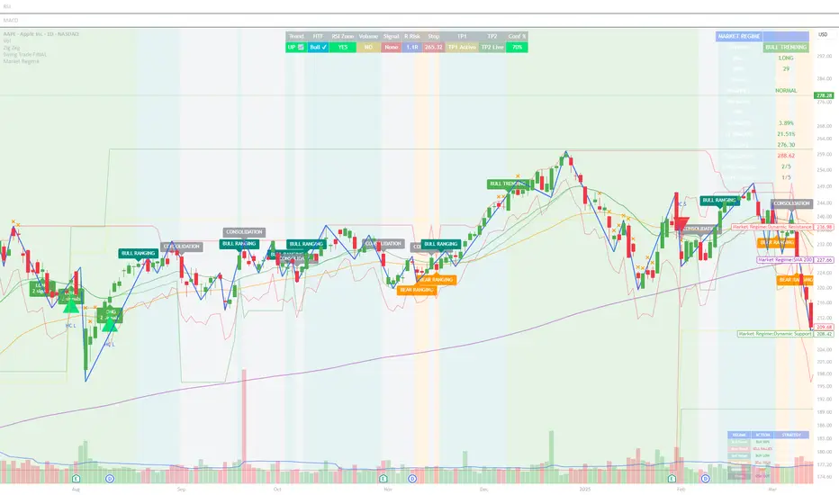
COT IndexTHE HIDDEN INTELLIGENCE IN FUTURES MARKETS
What if you could see what the smartest players in the futures markets are doing before the crowd catches on? While retail traders chase momentum indicators and moving averages, obsess over Japanese candlestick patterns, and debate whether the RSI should be set to fourteen or twenty-one periods, institutional players leave footprints in the sand through their mandatory reporting to the Commodity Futures Trading Commission. These footprints, published weekly in the Commitment of Traders reports, have been hiding in plain sight for decades, available to anyone with an internet connection, yet remarkably few traders understand how to interpret them correctly. The COT Index indicator transforms this raw institutional positioning data into actionable trading signals, bringing Wall Street intelligence to your trading screen without requiring expensive Bloomberg terminals or insider connections.
The uncomfortable truth is this: Most retail traders operate in a binary world. Long or short. Buy or sell. They apply technical analysis to individual positions, constrained by limited capital that forces them to concentrate risk in single directional bets. Meanwhile, institutional traders operate in an entirely different dimension. They manage portfolios dynamically weighted across multiple markets, adjusting exposure based on evolving market conditions, correlation shifts, and risk assessments that retail traders never see. A hedge fund might be simultaneously long gold, short oil, neutral on copper, and overweight agricultural commodities, with position sizes calibrated to volatility and portfolio Greeks. When they increase gold exposure from five percent to eight percent of portfolio allocation, this rebalancing decision reflects sophisticated analysis of opportunity cost, risk parity, and cross-market dynamics that no individual chart pattern can capture.
This portfolio reweighting activity, multiplied across hundreds of institutional participants, manifests in the aggregate positioning data published weekly by the CFTC. The Commitment of Traders report does not show individual trades or strategies. It shows the collective footprint of how actual commercial hedgers and large speculators have allocated their capital across different markets. When mining companies collectively increase forward gold sales to hedge thirty percent more production than last quarter, they are not reacting to a moving average crossover. They are making strategic allocation decisions based on production forecasts, cost structures, and price expectations derived from operational realities invisible to outside observers. This is portfolio management in action, revealed through positioning data rather than price charts.
If you want to understand how institutional capital actually flows, how sophisticated traders genuinely position themselves across market cycles, the COT report provides a rare window into that hidden world. But understand what you are getting into. This is not a tool for scalpers seeking confirmation of the next five-minute move. This is not an oscillator that flashes oversold at market bottoms with convenient precision. COT analysis operates on a timescale measured in weeks and months, revealing positioning shifts that precede major market turns but offer no precision timing. The data arrives three days stale, published only once per week, capturing strategic positioning rather than tactical entries.
If you need instant gratification, if you trade intraday moves, if you demand mechanical signals with ninety percent accuracy, close this document now. COT analysis rewards patience, position sizing discipline, and tolerance for being early. It punishes impatience, overleveraging, and the expectation that any single indicator can substitute for market understanding.
The premise is deceptively simple. Every Tuesday, large traders in futures markets must report their positions to the CFTC. By Friday afternoon, this data becomes public. Academic research spanning three decades has consistently shown that not all market participants are created equal. Some traders consistently profit while others consistently lose. Some anticipate major turning points while others chase trends into exhaustion. Bessembinder and Chan (1992) demonstrated in their seminal study that commercial hedgers, those with actual exposure to the underlying commodity or financial instrument, possess superior forecasting ability compared to speculators. Their research, published in the Journal of Finance, found statistically significant predictive power in commercial positioning, particularly at extreme levels. This finding challenged the efficient market hypothesis and opened the door to a new approach to market analysis based on positioning rather than price alone.
Think about what this means. Every week, the government publishes a report showing you exactly how the most informed market participants are positioned. Not their opinions. Not their predictions. Their actual money at risk. When agricultural producers collectively hold their largest short hedge in five years, they are not making idle speculation. They are locking in prices for crops they will harvest, informed by private knowledge of weather conditions, soil quality, inventory levels, and demand expectations invisible to outside observers. When energy companies aggressively hedge forward production at current prices, they reveal information about expected supply that no analyst report can capture. This is not technical analysis based on past prices. This is not fundamental analysis based on publicly available data. This is behavioral analysis based on how the smartest money is actually positioned, how institutions allocate capital across portfolios, and how those allocation decisions shift as market conditions evolve.
WHY SOME TRADERS KNOW MORE THAN OTHERS
Building on this foundation, Sanders, Boris and Manfredo (2004) conducted extensive research examining the behaviour patterns of different trader categories. Their work, which analyzed over a decade of COT data across multiple commodity markets, revealed a fascinating dynamic that challenges much of what retail traders are taught. Commercial hedgers consistently positioned themselves against market extremes, buying when speculators were most bearish and selling when speculators reached peak bullishness. The contrarian positioning of commercials was not random noise but rather reflected their superior information about supply and demand fundamentals. Meanwhile, large speculators, primarily hedge funds and commodity trading advisors, exhibited strong trend-following behaviour that often amplified market moves beyond fundamental values. Small traders, the retail participants, consistently entered positions late in trends, frequently near turning points, making them reliable contrary indicators.
Wang (2003) extended this research by demonstrating that the predictive power of commercial positioning varies significantly across different commodity sectors. His analysis of agricultural commodities showed particularly strong forecasting ability, with commercial net positions explaining up to fifteen percent of return variance in subsequent weeks. This finding suggests that the informational advantages of hedgers are most pronounced in markets where physical supply and demand fundamentals dominate, as opposed to purely financial markets where information asymmetries are smaller. When a corn farmer hedges six months of expected harvest, that decision incorporates private observations about rainfall patterns, crop health, pest pressure, and local storage capacity that no distant analyst can match. When an oil refinery hedges crude oil purchases and gasoline sales simultaneously, the spread relationships reveal expectations about refining margins that reflect operational realities invisible in public data.
The theoretical mechanism underlying these empirical patterns relates to information asymmetry and different participant motivations. Commercial hedgers engage in futures markets not for speculative profit but to manage business risks. An agricultural producer selling forward six months of expected harvest is not making a bet on price direction but rather locking in revenue to facilitate financial planning and ensure business viability. However, this hedging activity necessarily incorporates private information about expected supply, inventory levels, weather conditions, and demand trends that the hedger observes through their commercial operations (Irwin and Sanders, 2012). When aggregated across many participants, this private information manifests in collective positioning.
Consider a gold mining company deciding how much forward production to hedge. Management must estimate ore grades, recovery rates, production costs, equipment reliability, labor availability, and dozens of other operational variables that determine whether locking in prices at current levels makes business sense. If the industry collectively hedges more aggressively than usual, it suggests either exceptional production expectations or concern about sustaining current price levels or combination of both. Either way, this positioning reveals information unavailable to speculators analyzing price charts and economic data. The hedger sees the physical reality behind the financial abstraction.
Large speculators operate under entirely different incentives and constraints. Commodity Trading Advisors managing billions in assets typically employ systematic, trend-following strategies that respond to price momentum rather than fundamental supply and demand. When crude oil rallies from sixty dollars to seventy dollars per barrel, these systems generate buy signals. As the rally continues to eighty dollars, position sizes increase. The strategy works brilliantly during sustained trends but becomes a liability at reversals. By the time oil reaches ninety dollars, trend-following funds are maximally long, having accumulated positions progressively throughout the rally. At this point, they represent not smart money anticipating further gains but rather crowded money vulnerable to reversal. Sanders, Boris and Manfredo (2004) documented this pattern across multiple energy markets, showing that extreme speculator positioning typically marked late-stage trend exhaustion rather than early-stage trend development.
Small traders, the retail participants who fall below reporting thresholds, display the weakest forecasting ability. Wang (2003) found that small trader positioning exhibited negative correlation with subsequent returns, meaning their aggregate positioning served as a reliable contrary indicator. The explanation combines several factors. Retail traders often lack the capital reserves to weather normal market volatility, leading to premature exits from positions that would eventually prove profitable. They tend to receive information through slower channels, entering trends after mainstream media coverage when institutional participants are preparing to exit. Perhaps most importantly, they trade with emotion, buying into euphoria and selling into panic at precisely the wrong times.
At major turning points, the three groups often position opposite each other with commercials extremely bearish, large speculators extremely bullish, and small traders piling into longs at the last moment. These high-divergence environments frequently precede increased volatility and trend reversals. The insiders with business exposure quietly exit as the momentum traders hit maximum capacity and retail enthusiasm peaks. Within weeks, the reversal begins, and positions unwind in the opposite sequence.
FROM RAW DATA TO ACTIONABLE SIGNALS
The COT Index indicator operationalizes these academic findings into a practical trading tool accessible through TradingView. At its core, the indicator normalizes net positioning data onto a zero to one hundred scale, creating what we call the COT Index. This normalization is critical because absolute position sizes vary dramatically across different futures contracts and over time. A commercial trader holding fifty thousand contracts net long in crude oil might be extremely bullish by historical standards, or it might be quite neutral depending on the context of total market size and historical ranges. Raw position numbers mean nothing without context. The COT Index solves this problem by calculating where current positioning stands relative to its range over a specified lookback period, typically two hundred fifty-two weeks or approximately five years of weekly data.
The mathematical transformation follows the methodology originally popularized by legendary trader Larry Williams, though the underlying concept appears in statistical normalization techniques across many fields. For any given trader category, we calculate the highest and lowest net position values over the lookback period, establishing the historical range for that specific market and trader group. Current positioning is then expressed as a percentage of this range, where zero represents the most bearish positioning ever seen in the lookback window and one hundred represents the most bullish extreme. A reading of fifty indicates positioning exactly in the middle of the historical range, suggesting neither extreme optimism nor pessimism relative to recent history (Williams and Noseworthy, 2009).
This index-based approach allows for meaningful comparison across different markets and time periods, overcoming the scaling problems inherent in analyzing raw position data. A commercial index reading of eighty-five in gold carries the same interpretive meaning as an eighty-five reading in wheat or crude oil, even though the absolute position sizes differ by orders of magnitude. This standardization enables systematic analysis across entire futures portfolios rather than requiring market-specific expertise for each contract.
The lookback period selection involves a fundamental tradeoff between responsiveness and stability. Shorter lookback periods, perhaps one hundred twenty-six weeks or approximately two and a half years, make the index more sensitive to recent positioning changes. However, it also increases noise and produces more false signals. Longer lookback periods, perhaps five hundred weeks or approximately ten years, create smoother readings that filter short-term noise but become slower to recognize regime changes. The indicator settings allow users to adjust this parameter based on their trading timeframe, risk tolerance, and market characteristics.
UNDERSTANDING CFTC DATA STRUCTURES
The indicator supports both Legacy and Disaggregated COT report formats, reflecting the evolution of CFTC reporting standards over decades of market development. Legacy reports categorize market participants into three broad groups: commercial traders (hedgers with underlying business exposure), non-commercial traders (large speculators seeking profit without commercial interest), and non-reportable traders (small speculators below reporting thresholds). Each category brings distinct motivations and information advantages to the market (CFTC, 2020).
The Disaggregated reports, introduced in September 2009 for physical commodity markets, provide finer granularity by splitting participants into five categories (CFTC, 2009). Producer and merchant positions capture those actually producing, processing, or merchandising the physical commodity. Swap dealers represent financial intermediaries facilitating derivative transactions for clients. Managed money includes commodity trading advisors and hedge funds executing systematic or discretionary strategies. Other reportables encompasses diverse participants not fitting the main categories. Small traders remain as the fifth group, representing retail participation.
This enhanced categorization reveals nuances invisible in Legacy reports, particularly distinguishing between different types of institutional capital and their distinct behavioural patterns. The indicator automatically detects which report type is appropriate for each futures contract and adjusts the display accordingly.
Importantly, Disaggregated reports exist only for physical commodity futures. Agricultural commodities like corn, wheat, and soybeans have Disaggregated reports because clear producer, merchant, and swap dealer categories exist. Energy commodities like crude oil and natural gas similarly have well-defined commercial hedger categories. Metals including gold, silver, and copper also receive Disaggregated treatment (CFTC, 2009). However, financial futures such as equity index futures, Treasury bond futures, and currency futures remain available only in Legacy format. The CFTC has indicated no plans to extend Disaggregated reporting to financial futures due to different market structures and participant categories in these instruments (CFTC, 2020).
THE BEHAVIORAL FOUNDATION
Understanding which trader perspective to follow requires appreciation of their distinct trading styles, success rates, and psychological profiles. Commercial hedgers exhibit anticyclical behaviour rooted in their fundamental knowledge and business imperatives. When agricultural producers hedge forward sales during harvest season, they are not speculating on price direction but rather locking in revenue for crops they will harvest. Their business requires converting volatile commodity exposure into predictable cash flows to facilitate planning and ensure survival through difficult periods. Yet their aggregate positioning reveals valuable information because these hedging decisions incorporate private information about supply conditions, inventory levels, weather observations, and demand expectations that hedgers observe through their commercial operations (Bessembinder and Chan, 1992).
Consider a practical example from energy markets. Major oil companies continuously hedge portions of forward production based on price levels, operational costs, and financial planning needs. When crude oil trades at ninety dollars per barrel, they might aggressively hedge the next twelve months of production, locking in prices that provide comfortable profit margins above their extraction costs. This hedging appears as short positioning in COT reports. If oil rallies further to one hundred dollars, they hedge even more aggressively, viewing these prices as exceptional opportunities to secure revenue. Their short positioning grows increasingly extreme. To an outside observer watching only price charts, the rally suggests bullishness. But the commercial positioning reveals that the actual producers of oil find these prices attractive enough to lock in years of sales, suggesting skepticism about sustaining even higher levels. When the eventual reversal occurs and oil declines back to eighty dollars, the commercials who hedged at ninety and one hundred dollars profit while speculators who chased the rally suffer losses.
Large speculators or managed money traders operate under entirely different incentives and constraints. Their systematic, momentum-driven strategies mean they amplify existing trends rather than anticipate reversals. Trend-following systems, the most common approach among large speculators, by definition require confirmation of trend through price momentum before entering positions (Sanders, Boris and Manfredo, 2004). When crude oil rallies from sixty dollars to eighty dollars per barrel over several months, trend-following algorithms generate buy signals based on moving average crossovers, breakouts, and other momentum indicators. As the rally continues, position sizes increase according to the systematic rules.
However, this approach becomes a liability at turning points. By the time oil reaches ninety dollars after a sustained rally, trend-following funds are maximally long, having accumulated positions progressively throughout the move. At this point, their positioning does not predict continued strength. Rather, it often marks late-stage trend exhaustion. The psychological and mechanical explanation is straightforward. Trend followers by definition chase price momentum, entering positions after trends establish rather than anticipating them. Eventually, they become fully invested just as the trend nears completion, leaving no incremental buying power to sustain the rally. When the first signs of reversal appear, systematic stops trigger, creating a cascade of selling that accelerates the downturn.
Small traders consistently display the weakest track record across academic studies. Wang (2003) found that small trader positioning exhibited negative correlation with subsequent returns in his analysis across multiple commodity markets. This result means that whatever small traders collectively do, the opposite typically proves profitable. The explanation for small trader underperformance combines several factors documented in behavioral finance literature. Retail traders often lack the capital reserves to weather normal market volatility, leading to premature exits from positions that would eventually prove profitable. They tend to receive information through slower channels, learning about commodity trends through mainstream media coverage that arrives after institutional participants have already positioned. Perhaps most importantly, retail traders are more susceptible to emotional decision-making, buying into euphoria and selling into panic at precisely the wrong times (Tharp, 2008).
SETTINGS, THRESHOLDS, AND SIGNAL GENERATION
The practical implementation of the COT Index requires understanding several key features and settings that users can adjust to match their trading style, timeframe, and risk tolerance. The lookback period determines the time window for calculating historical ranges. The default setting of two hundred fifty-two bars represents approximately one year on daily charts or five years on weekly charts, balancing responsiveness with stability. Conservative traders seeking only the most extreme, highest-probability signals might extend the lookback to five hundred bars or more. Aggressive traders seeking earlier entry and willing to accept more false positives might reduce it to one hundred twenty-six bars or even less for shorter-term applications.
The bullish and bearish thresholds define signal generation levels. Default settings of eighty and twenty respectively reflect academic research suggesting meaningful information content at these extremes. Readings above eighty indicate positioning in the top quintile of the historical range, representing genuine extremes rather than temporary fluctuations. Conversely, readings below twenty occupy the bottom quintile, indicating unusually bearish positioning (Briese, 2008).
However, traders must recognize that appropriate thresholds vary by market, trader category, and personal risk tolerance. Some futures markets exhibit wider positioning swings than others due to seasonal patterns, volatility characteristics, or participant behavior. Conservative traders seeking high-probability setups with fewer signals might raise thresholds to eighty-five and fifteen. Aggressive traders willing to accept more false positives for earlier entry could lower them to seventy-five and twenty-five.
The key is maintaining meaningful differentiation between bullish, neutral, and bearish zones. The default settings of eighty and twenty create a clear three-zone structure. Readings from zero to twenty represent bearish territory where the selected trader group holds unusually bearish positions. Readings from twenty to eighty represent neutral territory where positioning falls within normal historical ranges. Readings from eighty to one hundred represent bullish territory where the selected trader group holds unusually bullish positions.
The trading perspective selection determines which participant group the indicator follows, fundamentally shaping interpretation and signal meaning. For counter-trend traders seeking reversal opportunities, monitoring commercial positioning makes intuitive sense based on the academic research discussed earlier. When commercials reach extreme bearish readings below twenty, indicating unprecedented short positioning relative to recent history, they are effectively betting against the crowd. Given their informational advantages demonstrated by Bessembinder and Chan (1992), this contrarian stance often precedes major bottoms.
Trend followers might instead monitor large speculator positioning, but with inverted logic compared to commercials. When managed money reaches extreme bullish readings above eighty, the trend may be exhausting rather than accelerating. This seeming paradox reflects their late-cycle participation documented by Sanders, Boris and Manfredo (2004). Sophisticated traders thus use speculator extremes as fade signals, entering positions opposite to speculator consensus.
Small trader monitoring serves primarily as a contrary indicator for all trading styles. Extreme small trader bullishness above seventy-five or eighty typically warns of retail FOMO at market tops. Extreme small trader bearishness below twenty or twenty-five often marks capitulation bottoms where the last weak hands have sold.
VISUALIZATION AND USER INTERFACE
The visual design incorporates multiple elements working together to facilitate decision-making and maintain situational awareness during active trading. The primary COT Index line plots in bold with adjustable line width, defaulting to two pixels for clear visibility against busy price charts. An optional glow effect, controlled by a simple toggle, adds additional visual prominence through multiple plot layers with progressively increasing transparency and width.
A twenty-one period exponential moving average overlays the index line, providing trend context for positioning changes. When the index crosses above its moving average, it signals accelerating bullish sentiment among the selected trader group regardless of whether absolute positioning is extreme. Conversely, when the index crosses below its moving average, it signals deteriorating sentiment and potentially the beginning of a reversal in positioning trends.
The EMA provides a dynamic reference line for assessing positioning momentum. When the index trades far above its EMA, positioning is not only extreme in absolute terms but also building with momentum. When the index trades far below its EMA, positioning is contracting or reversing, which may indicate weakening conviction even if absolute levels remain elevated.
The data table positioned at the top right of the chart displays eleven metrics for each trader category, transforming the indicator from a simple index calculation into an analytical dashboard providing multidimensional market intelligence. Beyond the COT Index itself, users can monitor positioning extremity, which measures how unusual current levels are compared to historical norms using statistical techniques. The extremity metric clarifies whether a reading represents the ninety-fifth or ninety-ninth percentile, with values above two standard deviations indicating genuinely exceptional positioning.
Market power quantifies each group's influence on total open interest. This metric expresses each trader category's net position as a percentage of total market open interest. A commercial entity holding forty percent of total open interest commands significantly more influence than one holding five percent, making their positioning signals more meaningful.
Momentum and rate of change metrics reveal whether positions are building or contracting, providing early warning of potential regime shifts. Position velocity measures the rate of change in positioning changes, effectively a second derivative providing even earlier insight into inflection points.
Sentiment divergence highlights disagreements between commercial and speculative positioning. This metric calculates the absolute difference between normalized commercial and large speculator index values. Wang (2003) found that these high-divergence environments frequently preceded increased volatility and reversals.
The table also displays concentration metrics when available, showing how positioning is distributed among the largest handful of traders in each category. High concentration indicates a few dominant players controlling most of the positioning, while low concentration suggests broad-based participation across many traders.
THE ALERT SYSTEM AND MONITORING
The alert system, comprising five distinct alert conditions, enables systematic monitoring of dozens of futures markets without constant screen watching. The bullish and bearish COT signal alerts trigger when the index crosses user-defined thresholds, indicating the selected trader group has reached extreme positioning worthy of attention. These alerts fire in real-time as new weekly COT data publishes, typically Friday afternoon following the Tuesday measurement date.
Extreme positioning alerts fire at ninety and ten index levels, representing the top and bottom ten percent of the historical range, warning of particularly stretched readings that historically precede reversals with high probability. When commercials reach a COT Index reading below ten, they are expressing their most bearish stance in the entire lookback period.
The data staleness alert notifies users when COT reports have not updated for more than ten days, preventing reliance on outdated information for trading decisions. Government shutdowns or federal holidays can interrupt the normal Friday publication schedule. Using stale signals while believing them current creates dangerous false confidence.
The indicator's watermark information display positioned in the bottom right corner provides essential context at a glance. This persistent display shows the symbol and timeframe, the COT report date timestamp, days since last update, and the current signal state. A trader analyzing a potential short entry in crude oil can glance at the watermark to instantly confirm positioning context without interrupting analysis flow.
LIMITATIONS AND REALISTIC EXPECTATIONS
Practical application requires understanding both the indicator's considerable strengths and inherent limitations. COT data inherently lags price action by three days, as Tuesday positions are not published until Friday afternoon. This delay means the indicator cannot catch rapid intraday reversals or respond to surprise news events. Traders using the COT Index for timing entries must accept this latency and focus on swing trading and position trading timeframes where three-day lags matter less than in day trading or scalping.
The weekly publication schedule similarly makes the indicator unsuitable for short-term trading strategies requiring immediate feedback. The COT Index works best for traders operating on weekly or longer timeframes, where positioning shifts measured in weeks and months align with trading horizon.
Extreme COT readings can persist far longer than typical technical indicators suggest, testing the patience and capital reserves of traders attempting to fade them. When crude oil enters a sustained bull market driven by genuine supply disruptions, commercial hedgers may maintain bearish positioning for many months as prices grind higher. A commercial COT Index reading of fifteen indicating extreme bearishness might persist for three months while prices continue rallying before finally reversing. Traders without sufficient capital and risk tolerance to weather such drawdowns will exit prematurely, precisely when the signal is about to work (Irwin and Sanders, 2012).
Position sizing discipline becomes paramount when implementing COT-based strategies. Rather than risking large percentages of capital on individual signals, successful COT traders typically allocate modest position sizes across multiple signals, allowing some to take time to mature while others work more quickly.
The indicator also cannot overcome fundamental regime changes that alter the structural drivers of markets. If gold enters a true secular bull market driven by monetary debasement, commercial hedgers may remain persistently bearish as mining companies sell forward years of production at what they perceive as favorable prices. Their positioning indicates valuation concerns from a production cost perspective, but cannot stop prices from rising if investment demand overwhelms physical supply-demand balance.
Similarly, structural changes in market participation can alter the meaning of positioning extremes. The growth of commodity index investing in the two thousands brought massive passive long-only capital into futures markets, fundamentally changing typical positioning ranges. Traders relying on COT signals without recognizing this regime change would have generated numerous false bearish signals during the commodity supercycle from 2003 to 2008.
The research foundation supporting COT analysis derives primarily from commodity markets where the commercial hedger information advantage is most pronounced. Studies specifically examining financial futures like equity indices and bonds show weaker but still present effects. Traders should calibrate expectations accordingly, recognizing that COT analysis likely works better for crude oil, natural gas, corn, and wheat than for the S&P 500, Treasury bonds, or currency futures.
Another important limitation involves the reporting threshold structure. Not all market participants appear in COT data, only those holding positions above specified minimums. In markets dominated by a few large players, concentration metrics become critical for proper interpretation. A single large trader accounting for thirty percent of commercial positioning might skew the entire category if their individual circumstances are idiosyncratic rather than representative.
GOLD FUTURES DURING A HYPOTHETICAL MARKET CYCLE
Consider a practical example using gold futures during a hypothetical but realistic market scenario that illustrates how the COT Index indicator guides trading decisions through a complete market cycle. Suppose gold has rallied from fifteen hundred to nineteen hundred dollars per ounce over six months, driven by inflation concerns following aggressive monetary expansion, geopolitical uncertainty, and sustained buying by Asian central banks for reserve diversification.
Large speculators, operating primarily trend-following strategies, have accumulated increasingly bullish positions throughout this rally. Their COT Index has climbed progressively from forty-five to eighty-five. The table display shows that large speculators now hold net long positions representing thirty-two percent of total open interest, their highest in four years. Momentum indicators show positive readings, indicating positions are still building though at a decelerating rate. Position velocity has turned negative, suggesting the pace of position building is slowing.
Meanwhile, commercial hedgers have responded to the rally by aggressively selling forward production and inventory. Their COT Index has moved inversely to price, declining from fifty-five to twenty. This bearish commercial positioning represents mining companies locking in forward sales at prices they view as attractive relative to production costs. The table shows commercials now hold net short positions representing twenty-nine percent of total open interest, their most bearish stance in five years. Concentration metrics indicate this positioning is broadly distributed across many commercial entities, suggesting the bearish stance reflects collective industry view rather than idiosyncratic positioning by a single firm.
Small traders, attracted by mainstream financial media coverage of gold's impressive rally, have recently piled into long positions. Their COT Index has jumped from forty-five to seventy-eight as retail investors chase the trend. Television financial networks feature frequent segments on gold with bullish guests. Internet forums and social media show surging retail interest. This retail enthusiasm historically marks late-stage trend development rather than early opportunity.
The COT Index indicator, configured to monitor commercial positioning from a contrarian perspective, displays a clear bearish signal given the extreme commercial short positioning. The table displays multiple confirming metrics: positioning extremity shows commercials at the ninety-sixth percentile of bearishness, market power indicates they control twenty-nine percent of open interest, and sentiment divergence registers sixty-five, indicating massive disagreement between commercial hedgers and large speculators. This divergence, the highest in three years, places the market in the historically high-risk category for reversals.
The interpretation requires nuance and consideration of context beyond just COT data. Commercials are not necessarily predicting an imminent crash. Rather, they are hedging business operations at what they collectively view as favorable price levels. However, the data reveals they have sold unusually large quantities of forward production, suggesting either exceptional production expectations for the year ahead or concern about sustaining current price levels or combination of both. Combined with extreme speculator positioning indicating a crowded long trade, and small trader enthusiasm confirming retail FOMO, the confluence suggests elevated reversal risk even if the precise timing remains uncertain.
A prudent trader analyzing this situation might take several actions based on COT Index signals. Existing long positions could be tightened with closer stop losses. Profit-taking on a portion of long exposure could lock in gains while maintaining some participation. Some traders might initiate modest short positions as portfolio hedges, sizing them appropriately for the inherent uncertainty in timing reversals. Others might simply move to the sidelines, avoiding new long entries until positioning normalizes.
The key lesson from case study analysis is that COT signals provide probabilistic edges rather than deterministic predictions. They work over many observations by identifying higher-probability configurations, not by generating perfect calls on individual trades. A fifty-five percent win rate with proper risk management produces substantial profits over time, yet still means forty-five percent of signals will be premature or wrong. Traders must embrace this probabilistic reality rather than seeking the impossible goal of perfect accuracy.
INTEGRATION WITH TRADING SYSTEMS
Integration with existing trading systems represents a natural and powerful use case for COT analysis, adding a positioning dimension to price-based technical approaches or fundamental analytical frameworks. Few traders rely exclusively on a single indicator or methodology. Rather, they build systems that synthesize multiple information sources, with each component addressing different aspects of market behavior.
Trend followers might use COT extremes as regime filters, modifying position sizing or avoiding new trend entries when positioning reaches levels historically associated with reversals. Consider a classic trend-following system based on moving average crossovers and momentum breakouts. Integration of COT analysis adds nuance. When large speculator positioning exceeds ninety or commercial positioning falls below ten, the regime filter recognizes elevated reversal risk. The system might reduce position sizing by fifty percent for new signals during these high-risk periods (Kaufman, 2013).
Mean reversion traders might require COT signal confluence before fading extended moves. When crude oil becomes technically overbought and large speculators show extreme long positioning above eighty-five, both signals confirm. If only technical indicators show extremes while positioning remains neutral, the potential short signal is rejected, avoiding fades of trends with underlying institutional support (Kaufman, 2013).
Discretionary traders can monitor the indicator as a continuous awareness tool, informing bias and position sizing without dictating mechanical entries and exits. A discretionary trader might notice commercial positioning shifting from neutral to progressively more bullish over several months. This trend informs growing positive bias even without triggering mechanical signals.
Multi-timeframe analysis represents another powerful integration approach. A trader might use daily charts for trade execution and timing while monitoring weekly COT positioning for strategic context. When both timeframes align, highest-probability opportunities emerge.
Portfolio construction for futures traders can incorporate COT signals as an additional selection criterion. Markets showing strong technical setups AND favorable COT positioning receive highest allocations. Markets with strong technicals but neutral or unfavorable positioning receive reduced allocations.
ADVANCED METRICS AND INTERPRETATION
The metrics table transforms simple positioning data into multidimensional market intelligence. Position extremity, calculated as the absolute deviation from the historical mean normalized by standard deviation, helps identify truly unusual readings versus routine fluctuations. A reading above two standard deviations indicates ninety-fifth percentile or higher extremity. Above three standard deviations indicates ninety-ninth percentile or higher, genuinely rare positioning that historically precedes major events with high probability.
Market power, expressed as a percentage of total open interest, reveals whose positioning matters most from a mechanical market impact perspective. Consider two scenarios in gold futures. In scenario one, commercials show a COT Index reading of fifteen while their market power metric shows they hold net shorts representing thirty-five percent of open interest. This is a high-confidence bearish signal. In scenario two, commercials also show a reading of fifteen, but market power shows only eight percent. While positioning is extreme relative to this category's normal range, their limited market share means less mechanical influence on price.
The rate of change and momentum metrics highlight whether positions are accelerating or decelerating, often providing earlier warnings than absolute levels alone. A COT Index reading of seventy-five with rapidly building momentum suggests continued movement toward extremes. Conversely, a reading of eighty-five with decelerating or negative momentum indicates the positioning trend is exhausting.
Position velocity measures the rate of change in positioning changes, effectively a second derivative. When velocity shifts from positive to negative, it indicates that while positioning may still be growing, the pace of growth is slowing. This deceleration often precedes actual reversal in positioning direction by several weeks.
Sentiment divergence calculates the absolute difference between normalized commercial and large speculator index values. When commercials show extreme bearish positioning at twenty while large speculators show extreme bullish positioning at eighty, the divergence reaches sixty, representing near-maximum disagreement. Wang (2003) found that these high-divergence environments frequently preceded increased volatility and reversals. The mechanism is intuitive. Extreme divergence indicates the informed hedgers and momentum-following speculators have positioned opposite each other with conviction. One group will prove correct and profit while the other proves incorrect and suffers losses. The resolution of this disagreement through price movement often involves volatility.
The table also displays concentration metrics when available. High concentration indicates a few dominant players controlling most of the positioning within a category, while low concentration suggests broad-based participation. Broad-based positioning more reliably reflects collective market intelligence and industry consensus. If mining companies globally all independently decide to hedge aggressively at similar price levels, it suggests genuine industry-wide view about price valuations rather than circumstances specific to one firm.
DATA QUALITY AND RELIABILITY
The CFTC has maintained COT reporting in various forms since the nineteen twenties, providing nearly a century of positioning data across multiple market cycles. However, data quality and reporting standards have evolved substantially over this long period. Modern electronic reporting implemented in the late nineteen nineties and early two thousands significantly improved accuracy and timeliness compared to earlier paper-based systems.
Traders should understand that COT reports capture positions as of Tuesday's close each week. Markets remain open three additional days before publication on Friday afternoon, meaning the reported data is three days stale when received. During periods of rapid market movement or major news events, this lag can be significant. The indicator addresses this limitation by including timestamp information and staleness warnings.
The three-day lag creates particular challenges during extreme volatility episodes. Flash crashes, surprise central bank interventions, geopolitical shocks, and other high-impact events can completely transform market positioning within hours. Traders must exercise judgment about whether reported positioning remains relevant given intervening events.
Reporting thresholds also mean that not all market participants appear in disaggregated COT data. Traders holding positions below specified minimums aggregate into the non-reportable or small trader category. This aggregation affects different markets differently. In highly liquid contracts like crude oil with thousands of participants, reportable traders might represent seventy to eighty percent of open interest. In thinly traded contracts with only dozens of active participants, a few large reportable positions might represent ninety-five percent of open interest.
Another data quality consideration involves trader classification into categories. The CFTC assigns traders to commercial or non-commercial categories based on reported business purpose and activities. However, this process is not perfect. Some entities engage in both commercial and speculative activities, creating ambiguity about proper classification. The transition to Disaggregated reports attempted to address some of these ambiguities by creating more granular categories.
COMPARISON WITH ALTERNATIVE APPROACHES
Several alternative approaches to COT analysis exist in the trading community beyond the normalization methodology employed by this indicator. Some analysts focus on absolute position changes week-over-week rather than index-based normalization. This approach calculates the change in net positioning from one week to the next. The emphasis falls on momentum in positioning changes rather than absolute levels relative to history. This method potentially identifies regime shifts earlier but sacrifices cross-market comparability (Briese, 2008).
Other practitioners employ more complex statistical transformations including percentile rankings, z-score standardization, and machine learning classification algorithms. Ruan and Zhang (2018) demonstrated that machine learning models applied to COT data could achieve modest improvements in forecasting accuracy compared to simple threshold-based approaches. However, these gains came at the cost of interpretability and implementation complexity.
The COT Index indicator intentionally employs a relatively straightforward normalization methodology for several important reasons. First, transparency enhances user understanding and trust. Traders can verify calculations manually and develop intuitive feel for what different readings mean. Second, academic research suggests that most of the predictive power in COT data comes from extreme positioning levels rather than subtle patterns requiring complex statistical methods to detect. Third, robust methods that work consistently across many markets and time periods tend to be simpler rather than more complex, reducing the risk of overfitting to historical data. Fourth, the complexity costs of implementation matter for retail traders without programming teams or computational infrastructure.
PSYCHOLOGICAL ASPECTS OF COT TRADING
Trading based on COT data requires psychological fortitude that differs from momentum-based approaches. Contrarian positioning signals inherently mean betting against prevailing market sentiment and recent price action. When commercials reach extreme bearish positioning, prices have typically been rising, sometimes for extended periods. The price chart looks bullish, momentum indicators confirm strength, moving averages align positively. The COT signal says bet against all of this. This psychological difficulty explains why COT analysis remains underutilized relative to trend-following methods.
Human psychology strongly predisposes us toward extrapolation and recency bias. When prices rally for months, our pattern-matching brains naturally expect continued rally. The recent price action dominates our perception, overwhelming rational analysis about positioning extremes and historical probabilities. The COT signal asking us to sell requires overriding these powerful psychological impulses.
The indicator design attempts to support the required psychological discipline through several features. Clear threshold markers and signal states reduce ambiguity about when signals trigger. When the commercial index crosses below twenty, the signal is explicit and unambiguous. The background shifts to red, the signal label displays bearish, and alerts fire. This explicitness helps traders act on signals rather than waiting for additional confirmation that may never arrive.
The metrics table provides analytical justification for contrarian positions, helping traders maintain conviction during inevitable periods of adverse price movement. When a trader enters short positions based on extreme commercial bearish positioning but prices continue rallying for several weeks, doubt naturally emerges. The table display provides reassurance. Commercial positioning remains extremely bearish. Divergence remains high. The positioning thesis remains intact even though price action has not yet confirmed.
Alert functionality ensures traders do not miss signals due to inattention while also not requiring constant monitoring that can lead to emotional decision-making. Setting alerts for COT extremes enables a healthier relationship with markets. When meaningful signals occur, alerts notify them. They can then calmly assess the situation and execute planned responses.
However, no indicator design can completely overcome the psychological difficulty of contrarian trading. Some traders simply cannot maintain short positions while prices rally. For these traders, COT analysis might be better employed as an exit signal for long positions rather than an entry signal for shorts.
Ultimately, successful COT trading requires developing comfort with probabilistic thinking rather than certainty-seeking. The signals work over many observations by identifying higher-probability configurations, not by generating perfect calls on individual trades. A fifty-five or sixty percent win rate with proper risk management produces substantial profits over years, yet still means forty to forty-five percent of signals will be premature or wrong. COT analysis provides genuine edge, but edge means probability advantage, not elimination of losing trades.
EDUCATIONAL RESOURCES AND CONTINUOUS LEARNING
The indicator provides extensive built-in educational resources through its documentation, detailed tooltips, and transparent calculations. However, mastering COT analysis requires study beyond any single tool or resource. Several excellent resources provide valuable extensions of the concepts covered in this guide.
Books and practitioner-focused monographs offer accessible entry points. Stephen Briese published The Commitments of Traders Bible in two thousand eight, offering detailed breakdowns of how different markets and trader categories behave (Briese, 2008). Briese's work stands out for its empirical focus and market-specific insights. Jack Schwager includes discussion of COT analysis within the broader context of market behavior in his book Market Sense and Nonsense (Schwager, 2012). Perry Kaufman's Trading Systems and Methods represents perhaps the most rigorous practitioner-focused text on systematic trading approaches including COT analysis (Kaufman, 2013).
Academic journal articles provide the rigorous statistical foundation underlying COT analysis. The Journal of Futures Markets regularly publishes research on positioning data and its predictive properties. Bessembinder and Chan's earlier work on systematic risk, hedging pressure, and risk premiums in futures markets provides theoretical foundation (Bessembinder, 1992). Chang's examination of speculator returns provides historical context (Chang, 1985). Irwin and Sanders provide essential skeptical perspective in their two thousand twelve article (Irwin and Sanders, 2012). Wang's two thousand three article provides one of the most empirical analyses of COT data across multiple commodity markets (Wang, 2003).
Online resources extend beyond academic and book-length treatments. The CFTC website provides free access to current and historical COT reports in multiple formats. The explanatory materials section offers detailed documentation of report construction, category definitions, and historical methodology changes. Traders serious about COT analysis should read these official CFTC documents to understand exactly what they are analyzing.
Commercial COT data services such as Barchart provide enhanced visualization and analysis tools beyond raw CFTC data. TradingView's educational materials, published scripts library, and user community provide additional resources for exploring different approaches to COT analysis.
The key to mastering COT analysis lies not in finding a single definitive source but rather in building understanding through multiple perspectives and information sources. Academic research provides rigorous empirical foundation. Practitioner-focused books offer practical implementation insights. Direct engagement with data through systematic backtesting develops intuition about how positioning dynamics manifest across different market conditions.
SYNTHESIZING KNOWLEDGE INTO PRACTICE
The COT Index indicator represents the synthesis of academic research, trading experience, and software engineering into a practical tool accessible to retail traders equipped with nothing more than a TradingView account and willingness to learn. What once required expensive data subscriptions, custom programming capabilities, statistical software, and institutional resources now appears as a straightforward indicator requiring only basic parameter selection and modest study to understand. This democratization of institutional-grade analysis tools represents a broader trend in financial markets over recent decades.
Yet technology and data access alone provide no edge without understanding and discipline. Markets remain relentlessly efficient at eliminating edges that become too widely known and mechanically exploited. The COT Index indicator succeeds only when users invest time learning the underlying concepts, understand the limitations and probability distributions involved, and integrate signals thoughtfully into trading plans rather than applying them mechanically.
The academic research demonstrates conclusively that institutional positioning contains genuine information about future price movements, particularly at extremes where commercial hedgers are maximally bearish or bullish relative to historical norms. This informational content is neither perfect nor deterministic but rather probabilistic, providing edge over many observations through identification of higher-probability configurations. Bessembinder and Chan's finding that commercial positioning explained modest but significant variance in future returns illustrates this probabilistic nature perfectly (Bessembinder and Chan, 1992). The effect is real and statistically significant, yet it explains perhaps ten to fifteen percent of return variance rather than most variance. Much of price movement remains unpredictable even with positioning intelligence.
The practical implication is that COT analysis works best as one component of a trading system rather than a standalone oracle. It provides the positioning dimension, revealing where the smart money has positioned and where the crowd has followed, but price action analysis provides the timing dimension. Fundamental analysis provides the catalyst dimension. Risk management provides the survival dimension. These components work together synergistically.
The indicator's design philosophy prioritizes transparency and education over black-box complexity, empowering traders to understand exactly what they are analyzing and why. Every calculation is documented and user-adjustable. The threshold markers, background coloring, tables, and clear signal states provide multiple reinforcing channels for conveying the same information.
This educational approach reflects a conviction that sustainable trading success comes from genuine understanding rather than mechanical system-following. Traders who understand why commercial positioning matters, how different trader categories behave, what positioning extremes signify, and where signals fit within probability distributions can adapt when market conditions change. Traders mechanically following black-box signals without comprehension abandon systems after normal losing streaks.
The research foundation supporting COT analysis comes primarily from commodity markets where commercial hedger informational advantages are most pronounced. Agricultural producers hedging crops know more about supply conditions than distant speculators. Energy companies hedging production know more about operating costs than financial traders. Metals miners hedging output know more about ore grades than index funds. Financial futures markets show weaker but still present effects.
The journey from reading this documentation to profitable trading based on COT analysis involves several stages that cannot be rushed. Initial reading and basic understanding represents the first stage. Historical study represents the second stage, reviewing past market cycles to observe how positioning extremes preceded major turning points. Paper trading or small-size real trading represents the third stage to experience the psychological challenges. Refinement based on results and personal psychology represents the fourth stage.
Markets will continue evolving. New participant categories will emerge. Regulatory structures will change. Technology will advance. Yet the fundamental dynamics driving COT analysis, that different market participants have different information, different motivations, and different forecasting abilities that manifest in their positioning, will persist as long as futures markets exist. While specific thresholds or optimal parameters may shift over time, the core logic remains sound and adaptable.
The trader equipped with this indicator, understanding of the theory and evidence behind COT analysis, realistic expectations about probability rather than certainty, discipline to maintain positions through adverse volatility, and patience to allow signals time to develop possesses genuine edge in markets. The edge is not enormous, markets cannot allow large persistent inefficiencies without arbitraging them away, but it is real, measurable, and exploitable by those willing to invest in learning and disciplined application.
REFERENCES
Bessembinder, H. (1992) Systematic risk, hedging pressure, and risk premiums in futures markets, Review of Financial Studies, 5(4), pp. 637-667.
Bessembinder, H. and Chan, K. (1992) The profitability of technical trading rules in the Asian stock markets, Pacific-Basin Finance Journal, 3(2-3), pp. 257-284.
Briese, S. (2008) The Commitments of Traders Bible: How to Profit from Insider Market Intelligence. Hoboken: John Wiley & Sons.
Chang, E.C. (1985) Returns to speculators and the theory of normal backwardation, Journal of Finance, 40(1), pp. 193-208.
Commodity Futures Trading Commission (CFTC) (2009) Explanatory Notes: Disaggregated Commitments of Traders Report. Available at: www.cftc.gov (Accessed: 15 January 2025).
Commodity Futures Trading Commission (CFTC) (2020) Commitments of Traders: About the Report. Available at: www.cftc.gov (Accessed: 15 January 2025).
Irwin, S.H. and Sanders, D.R. (2012) Testing the Masters Hypothesis in commodity futures markets, Energy Economics, 34(1), pp. 256-269.
Kaufman, P.J. (2013) Trading Systems and Methods. 5th edn. Hoboken: John Wiley & Sons.
Ruan, Y. and Zhang, Y. (2018) Forecasting commodity futures prices using machine learning: Evidence from the Chinese commodity futures market, Applied Economics Letters, 25(12), pp. 845-849.
Sanders, D.R., Boris, K. and Manfredo, M. (2004) Hedgers, funds, and small speculators in the energy futures markets: an analysis of the CFTC's Commitments of Traders reports, Energy Economics, 26(3), pp. 425-445.
Schwager, J.D. (2012) Market Sense and Nonsense: How the Markets Really Work and How They Don't. Hoboken: John Wiley & Sons.
Tharp, V.K. (2008) Super Trader: Make Consistent Profits in Good and Bad Markets. New York: McGraw-Hill.
Wang, C. (2003) The behavior and performance of major types of futures traders, Journal of Futures Markets, 23(1), pp. 1-31.
Williams, L.R. and Noseworthy, M. (2009) The Right Stock at the Right Time: Prospering in the Coming Good Years. Hoboken: John Wiley & Sons.
FURTHER READING
For traders seeking to deepen their understanding of COT analysis and futures market positioning beyond this documentation, the following resources provide valuable extensions:
Academic Journal Articles:
Fishe, R.P.H. and Smith, A. (2012) Do speculators drive commodity prices away from supply and demand fundamentals?, Journal of Commodity Markets, 1(1), pp. 1-16.
Haigh, M.S., Hranaiova, J. and Overdahl, J.A. (2007) Hedge funds, volatility, and liquidity provision in energy futures markets, Journal of Alternative Investments, 9(4), pp. 10-38.
Kocagil, A.E. (1997) Does futures speculation stabilize spot prices? Evidence from metals markets, Applied Financial Economics, 7(1), pp. 115-125.
Sanders, D.R. and Irwin, S.H. (2011) The impact of index funds in commodity futures markets: A systems approach, Journal of Alternative Investments, 14(1), pp. 40-49.
Books and Practitioner Resources:
Murphy, J.J. (1999) Technical Analysis of the Financial Markets: A Guide to Trading Methods and Applications. New York: New York Institute of Finance.
Pring, M.J. (2002) Technical Analysis Explained: The Investor's Guide to Spotting Investment Trends and Turning Points. 4th edn. New York: McGraw-Hill.
Federal Reserve and Research Institution Publications:
Federal Reserve Banks regularly publish working papers examining commodity markets, futures positioning, and price discovery mechanisms. The Federal Reserve Bank of San Francisco and Federal Reserve Bank of Kansas City maintain active research programs in this area.
Online Resources:
The CFTC website provides free access to current and historical COT reports, explanatory materials, and regulatory documentation.
Barchart offers enhanced COT data visualization and screening tools.
TradingView's community library contains numerous published scripts and educational materials exploring different approaches to positioning analysis.

AI x Meme Impulse Tracker [QuantraSystems]AI x Meme Impulse Tracker
Quantra Systems guarantees that the information created and published within this document and on the Tradingview platform is fully compliant with applicable regulations, does not constitute investment advice, and is not exclusively intended for qualified investors.
Important Note!
The system equity curve presented here has been generated as part of the process of testing and verifying the methodology behind this script.
Crucially, it was developed after the system was conceptualized, designed, and created, which helps to mitigate the risk of overfitting to historical data. In other words, the system was built for robustness, not for simply optimizing past performance.
This ensures that the system is less likely to degrade in performance over time, compared to hyper-optimized systems that are tailored to past data. No tweaks or optimizations were made to this system post-backtest.
Even More Important Note!!
The nature of markets is that they change quickly and unpredictably. Past performance does not guarantee future results - this is a fundamental rule in trading and investing.
While this system is designed with broad, flexible conditions to adapt quickly to a range of market environments, it is essential to understand that no assumptions should be made about future returns based on historical data. Markets are inherently uncertain, and this system - like all trading systems - cannot predict future outcomes.
Introduction
The AI x Meme Impulse Tracker is a cutting-edge, fast-acting rotational algorithm designed to capitalize on the strength of assets within pre-selected categories. Using a custom function built on top of the RSI Pulsar, the system measures momentum through impulses rather than traditional trend following methods. This allows for swifter reallocations based on short bursts of strength.
This system focuses on precision and agility - making it highly adaptable in volatile markets. The strategy is built around three independent asset categories - with allocations only made to the strongest asset in each - ensuring that capital movement (in particular between blockchains) is kept to a minimum for efficiency purposes while maintaining exposure to the highest performing tokens.
Legend
Token Inputs:
The Impulse Tracker is designed with dynamic asset selection - allowing traders to customize the inputs for each category. This feature enables flexible system management, as the number of active tokens within each category can be adjusted at any time. Whether the user chooses the default of 13 tokens per category, or fewer, the system will automatically recalibrate. This ensures that all calculations, from relative strength to individual performance assessments, adjust as required. Disabled tokens are treated by the system as if they don’t exist - seamlessly updating performance metrics and the Impulse Tracker’s allocation behavior to maintain the highest level of efficiency and accuracy.
System Equity Curve:
The Impulse Tracker plots both the rotational system’s equity and the Buy-and-Hold (or ‘HODL’) benchmark of Bitcoin for comparison. While the HODL approach allocates the entire portfolio to Bitcoin and functions as an index to compare to, the Impulse Tracker dynamically allocates based on strength impulses within the chosen tokens and categories. The system equity curve is representative of adding an equal capital split between the strongest assets of each category. The relative strength system does handle ‘ties’ of strength - in this situation multiple tokens from a single category can be included in the final equity curve, with the allocated weight to that category split between the tied assets.
TABLES:
Equity Stats:
This table is held in Quantra System's typical UI design language. It offers a comprehensive snapshot of the system’s performance, with key metrics organized to help traders quickly assess both short-term and cumulative results. The left side provides details on individual asset performance, while the right side presents a comparison of the system’s risk-adjusted metrics against a simple BTC Hodl strategy.
The leftmost column of the Equity Stats table showcases performance indicators for the system’s current allocations. This provides quick identification of the current strongest tokens, based on confirmed and non-repainting data as soon as the current opens and the last bar closes.
The right-hand side compares the performance differences between the system and Hodl profits, both on a cumulative basis and analyzing only the previous bar. The total number of position changes is also tracked in this table - an important metric when calculating total slippage and should be used to determine how ‘hands-on’ the strategy will be on the current timeframe.
The lower part of the table highlights a direct comparison of the AI x Memes Impulse strategy with buy-and-hold Bitcoin. The risk adjusted performance ratios, Sharpe, Sortino and Omega, are shown side by side, as well as the maximum drawdown experienced by both strategies within the set testing window.
Screener Table:
This table provides a detailed breakdown of the performance for each asset that has been the strongest in its category at some point and thus received an allocation. The table tracks several key metrics for each asset - including returns, volatility, Sharpe ratio, Sortino ratio, Omega ratio, and maximum drawdown. It also displays the signals for both current and previous periods, as well as the assets weight in the theoretical portfolio. Assets that have never received a signal are also included, giving traders an overview of which assets have contributed to the portfolio's performance and which have not played a role so far.
The position changes cell also offers important insights, as it shows the frequency of not just total position changes, but also rebalancing events.
Detailed Slippage Table:
The Detailed Slippage Table provides a comprehensive breakdown of the calculated slippage and fees incurred throughout the strategy’s operations. It contains several key metrics that give traders a granular view of the costs associated with executing the system:
Selected Slippage - Displays the current slippage rate, as defined in the input menu.
Removal Slippage - This accounts for any slippage or fees incurred when removing an allocation from a token.
Reallocation Slippage - Tracks the slippage or fees when reallocating capital to existing positions.
Addition Slippage - Measures the slippage or fees incurred when allocating capital to new tokens.
Final Slippage - Is the sum of all the individual slippage points and provides a quick view of the total slippage accounted for by the system.
The table is also divided into two columns:
Last Transaction Slippage + Fees - Displays any slippage or fees incurred based on position changes within the current bar.
Total Slippage + Fees - Shows the cumulative slippage and fees incurred since the portfolio’s selected start date.
Visual Customization:
Several customizable features are included within the input menu to enhance user experience. These include custom color palettes, both preloaded and user-selectable. This allows traders to personalize the visual appearance of the tables, ensuring clarity and consistency with their preferred interface themes and background coloring.
Additionally, users can adjust both the position and sizes of all the tables - enabling complete tailoring to the trader’s layout and specific viewing preferences and screen configurations. This level of customization ensures a more intuitive and flexible interaction with the system’s data.
Core Features and Methodologies
Advanced Risk Management - A Unique Filtering Approach:
The Equity Curve Activation Filter introduces an innovative way to dynamically manage capital allocation, aligning with periods of market trend strength. This filter is rooted in the understanding that markets move cyclically - altering between periods trending and mean-reverting periods. This cycle is especially pronounced in the crypto markets, where strong uptrends are often followed by prolonged periods of sideways movements or corrections as participants take profits and momentum fades.
The Cyclical Nature of Markets and Trend Following:
Financial markets do not trend indefinitely. Each uptrend or downtrend, whether over high and low timeframes, tends to culminate in a phase where momentum exhausts - leading to the sideways or corrective phases. This cycle results from the natural dynamics of market participants: during extended trends, more participants jump in, riding the momentum until profit taking causes the trend to slow down or reverse. This cyclical behavior occurs across all timeframes and in all markets - making it essential to adapt trading strategies in attempt to minimize losses during less favorable conditions.
In a trend following system, profitability often mirrors this cyclical pattern. Trend following strategies thrive when markets are moving directionally, capturing gains as price moves with strength in a single direction. However in phases where the market chops sideways, trend following strategies will usually experience drawdowns and reduced returns due to the impersistent nature of any trends. This fluctuation in trend following profitability can actually serve as one of the best coincident indicators of broader market regime change - when profitability begins to fade, it often signals a transition to drawn out unfavorable trend trading conditions.
The Equity Curve as a Market Signal
Within the Impulse Tracker, a continuous equity curve is calculated based upon the system's allocation to the strongest tokens. This equity curve effectively tracks the system’s performance under all market conditions. However, instead of solely relying on the direct performance of the selected tokens, the system applies additional filters to analyze the trend strength of this equity curve itself.
In the same way you only want to purchase an asset that is moving up in price, you only want to allocate capital to a strategy whose equity curve is trending upwards!
The Equity Curve Activation Filter consistently monitors the trend of this equity curve through various filter indicators, such as the “Wave Pendulum Trend”, the “Quasar QSM” and the “MAQSM” (an aggregate of multiple types of averages). These filters help determine whether the equity curve is trending upwards, signaling a favorable period for trend following. When the equity curve is in a positive trend, capital is allocated to the system as normal - allowing it to capture gains during favorable market conditions, Conversely, when the trend weakens and the equity curves begins to stagnate or decline, the activation filter shifts the system into a “cash” positions - temporarily halting allocations in order to prevent market exposure during choppy or mean reverting phases.
Timing Allocation With Market Conditions
This unique filtering approach ensures that the system is primarily active during periods when market trends are most supportive. By aligning capital allocations with the uptrend in trend following profitability, the system is designed to enter during periods of strong momentum and move to cash when momentum with the equity curve wanes. This approach reduces the risk of overtrading in less favorable conditions and preserves capital for the next favorable trend.
In essence the Equity Curve Allocation Filter serves as a dynamic risk management layer that leverages the cyclicality of trend following profitability in order to navigate shifting market phases.
Sensitivity and Signal Responsiveness:
The Quasar Sensitivity Setting allows users to fine-tune the system’s responsiveness to asset signals. High sensitivity settings lead to quicker position changes, making the system highly reactive to short term strength impulses. This is especially useful in fast moving markets where token strength can shift rapidly. The Sensitive setting might be more applicable to higher volatility or lower market cap assets - as the increased volatility increases the necessity of faster position cutting in order to front run the crowd. Of course - a balanced approach is ideal, as if the signals are too fast there will be too many whips and false signals. (And extra fees + slippage!)
The benefit of this script is because of the advanced slippage calculations, false signals are sufficiently punished (unlike systems without fees or slippage) - so it will become immediately apparent if the false signals have a significantly detrimental impact on the system’s equity curve.
Asset specific signals within each category are re-evaluated after the close of each bar to ensure that capital is always allocated to the highest performing asset. If a token’s momentum begins to fade the system swiftly reallocates to the next strongest asset within that category.
Category Filter - Allocates only to the Strongest Asset per group
One of the core innovations of the AI x Meme Impulse Tracker is the customizable Category Filter, which ensures that only the strongest-performing asset within each predefined group receives capital allocation. This approach not only increases the precision of asset selection but also allows traders to tailor the system to specific token narratives or categories. Sectors can include trending themes such as high-attention meme tokens, AI-driven tokens, or even categorize assets by blockchain ecosystems like Ethereum, Solana, or Base chain. This flexibility enables users to align their strategies with the latest market narratives or to optimize for specific groups, focusing on high-beta tokens within well defined sectors for a more targeted exposure. By keeping the focus on category leaders, the system avoids diluting its impact across underperforming assets, thereby maximizing capital efficiency and reducing unnecessary trading costs.
Dynamic Asset Reallocation:
Dynamic reallocation ensures that the system remains nimble and adapts to changing market conditions. Unlike slower systems, the Quasar method continually monitors for changes in asset strength and reallocates capital accordingly - ensuring that the system is always positioned in the highest performing assets within each category.
Position Changes and Slippage:
The Impulse Tracker places a strong emphasis on realistic simulation, prioritizing accuracy over inflated backtest results. This approach ensures that slippage is accounted for in a more aggressive manner than what may be experienced in real-world execution.
Each position change within the system - whether it’s buying, selling, reallocating, or rebalancing between assets - incurs slippage. Slippage is applied to both ends of every transaction: when a position is entered and exited, and when reallocating capital from one token to another. This dynamic behavior is further enhanced by a customizable slippage/fees input, allowing users to simulate realistic transaction costs based on their own market conditions and execution behaviors.
The slippage model works by applying a weighted slippage to the equity curve, taking into account the actual amount of capital being moved. Slippage is not applied in a blanket manner but rather in proportion to the allocation changes. For example, if the system reallocates from a single 100% position to two 50% allocations, slippage will be applied to the 50% removed from the first asset and the 50% added to the new asset, resulting in a 1x slippage multiplier.
This process becomes more granular when multiple assets are involved. For instance, if reallocating from two 50% positions to three 33% positions, slippage will be incurred on each of the changes, but at a reduced rate (⅔ x slippage), reflecting the smaller percentage of portfolio equity being moved. The slippage model accounts for all types of allocation shifts, whether increasing or decreasing the number of tokens held, providing a realistic assessment of system costs.
Here are some detailed examples to illustrate how slippage is calculated based on different scenarios:
100% → 50% / 50%: 1x slippage applied to both position changes (2 allocation changes).
50% / 50% → 33% / 33% / 33%: ⅔ x slippage multiplier applied across 3 allocation changes.
33% / 33% / 33% → 100%: 4/3 x slippage multiplier applied across 3 allocation changes.
In practice, not every position change will be rebalanced perfectly, leading to a lower number of transactions and lower costs in practice. Additionally, with the use of limit orders, a trader can easily reduce the costs of entering a position, as well as ensuring a competitive entry price.
By simulating slippage in this granular manner, the system captures the absolute maximum level of fees and slippage, in order to ensure that backtest results lean towards an underrepresentation - opposed to inflated results compared with practical execution.
A Special Note on Slippage
In the image above, the system has been applied to four different timeframes - 20h, 15h, 10h, and 5h - using identical settings and a selected slippage amount of 2%. By isolating a recent trend leg, we can illustrate an important concept: while the 15h timeframe is more profitable than the 20h timeframe, this difference stems from a core trading principle. Lower timeframes typically provide more data points and allow for quicker entries and exits in a robust system. This often results in reduced downside and compounding of gains.
However, slippage, fees, and execution constraints are limiting factors, especially in volatile, low-cap cryptocurrencies. Although lower timeframes can improve performance by increasing trade frequency, each trade incurs heavy slippage costs that accumulate - impacting the portfolio’s capital at a compounding rate. In this example, the chosen slippage rate of 2% per trade is designed to reflect the realistic trading costs, emphasizing how lower timeframe trading comes at the cost of increased slippage and fees
Finding the optimal balance between timeframe and slippage impact requires careful consideration of factors such as portfolio size, liquidity of selected tokens, execution speed, and the fee rate of the exchange you execute trades on.
Equity Curve and Performance Calculations
To provide a benchmark, the script also generates a Buy-and-Hold (or "HODL") equity curve that represents a complete allocation to Bitcoin. This allows users to easily compare the performance of the dynamic rotation system with that more traditional benchmark strategy.
The script tracks key performance metrics for both the dynamic portfolio and the HODL strategy, including:
Sharpe Ratio
The Sharpe Ratio is a key metric that evaluates a portfolio’s risk-adjusted return by comparing its ‘excess’ return to its volatility. Traditionally, the Sharpe Ratio measures returns relative to a risk-free rate. However, in our system’s calculation, we omit the risk-free rate and instead measure returns above a benchmark of 0%. This adjustment provides a more universal comparison, especially in the context of highly volatile assets like cryptocurrencies, where a traditional risk-free benchmark, such as the usual 3-month T-bills, is often irrelevant or too distant from the realities of the crypto market.
By using 0% as the baseline, we focus purely on the strategy's ability to generate raw returns in the face of market risk, which makes it easier to compare performance across different strategies or asset classes. In an environment like cryptocurrency, where volatility can be extreme, the importance of relative return against a highly volatile backdrop outweighs comparisons to a risk-free rate that bears little resemblance to the risk profile of digital assets.
Sortino Ratio
The Sortino Ratio improves upon the Sharpe Ratio by specifically targeting downside risk and leaves the upside potential untouched. In contrast to the Sharpe Ratio (which penalizes both upside and downside volatility), the Sortino Ratio focuses only on negative return deviations. This makes it a more suitable metric for evaluating strategies like the AI x Meme Impulse Tracker - that aim to minimize drawdowns without restricting upside capture. By measuring returns relative to a 0% baseline, the Sortino ratio provides a clearer assessment of how well the system generates gains while avoiding substantial losses in highly volatile markets like crypto.
Omega Ratio
The Omega Ratio is calculated as the ratio of gains to losses across all return thresholds, providing a more complete view of how the system balances upside and downside risk even compared to the Sortino Ratio. While it achieves a similar outcome to the Sortino Ratio by emphasizing the system's ability to capture gains while limiting losses, it is technically a mathematically superior method. However, we include both the Omega and Sortino ratios in our metric table, as the Sortino Ratio remains more widely recognized and commonly understood by traders and investors of all levels.
Usage Summary:
While the backtests in this description are generated as if a trader held a portfolio of just the strongest tokens, this was mainly designed as a method of logical verification and not a recommended investment strategy. In practice, this system can be used in multiple ways.
It can be used as above, or as a factor in forming part of a broader asset selection system, or even a method of filtering tokens by strength in order to inform a day trader which tokens might be optimal to look for long-only trading setups on an intrabar timeframe.
Final Summary:
The AI x Meme Impulse Tracker is a powerful algorithm that leverages a unique strength and impulse based approach to asset allocation within high beta token categories. Built with a robust risk management framework, the system’s Equity Curve Activation Filter dynamically manages capital exposure based on the cyclical nature of market trends, minimizing exposure during weaker phases.
With highly customizable settings, the Impulse Tracker enables precise capital allocation to only the strongest assets, informed by real-time metrics and rigorous slippage modeling in order to provide the best view of historical profitability. This adaptable design, coupled with advanced performance analytics, makes it a versatile tool for traders seeking an edge in fast moving and volatile crypto markets.
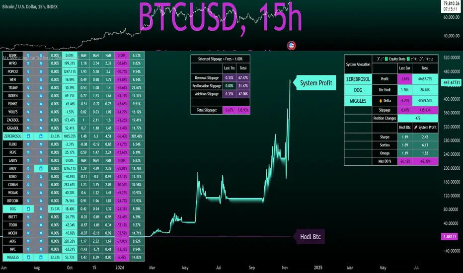
GKD-BT Optimizer SCSC Backtest [Loxx]The Giga Kaleidoscope GKD-BT Optimizer SCSC Backtest (Solo Confirmation Super Complex) is a Backtest module included in AlgxTrading's "Giga Kaleidoscope Modularized Trading System." (see the section Giga Kaleidoscope (GKD) Modularized Trading System below for an explanation of the GKD trading system)
**the backtest data rendered to the chart above and all screenshots below use $5 commission per trade and 10% equity per trade with $1 million initial capital**
█ GKD-BT Optimizer SCSC Backtest
The GKD-BT Optimizer SCSC Backtest is a comprehensive backtesting module designed to optimize the combination of key GKD indicators within AlgxTrading's "Giga Kaleidoscope Modularized Trading System." This module facilitates precise strategy refinement by allowing traders to configure and optimize the following critical GKD indicators:
GKD-B Baseline
GKD-V Volatility/Volume
GKD-C Confirmation 1
GKD-C Continuation
Each indicator is equipped with an "Optimizer" mode, enabling dynamic feedback and iterative improvements directly into the backtesting environment. This integrated approach ensures that each component contributes effectively to the overall strategy, providing a robust framework for achieving optimized trading outcomes.
The GKD-BT Optimizer supports granular test configurations including a single take profit and stop loss setting, and allows for targeted testing within specified date ranges to simulate forward testing with historical data. This feature is essential for evaluating the resilience and effectiveness of trading strategies under various market conditions.
Furthermore, the module is designed with user-centric features such as:
Customizable Trading Panel: Displays critical backtest results and trade statistics, which can be shown or hidden as per user preference.
Highlighting Thresholds: Users can set thresholds for Total Percent Wins, Percent Profitable, and Profit Factor, which helps in quickly identifying the most relevant metrics for analysis.
The detailed setup ensures that traders can not only adjust their strategies based on historical performance but also fine-tune their approach to meet specific trading objectives.
🔶 To configure this indicator: ***all GKD indicators listed below are all included in the AlgxTrading trading system package***
1. Add GKD-C Confirmation, GKD-B Baseline, GKD-V Volatility/Volume, and GKD-C Continuation to your chart
2. In the GKD-B Baseline indicator, change "Baseline Type" to "Optimizer"
3. In the GKD-V Volatility/Volume indicator, change "Volatility/Volume Type" to "Optimizer"
4. In the GKD-C Confirmation 1 indicator, change "Confirmation Type" to "Optimizer"
5. In the GKD-C Continuation indicator, change "Confirmation Type" to "Optimizer"
An example of steps 2-5. In the screenshot example below, we change the value "Confirmation Type" in the GKD-C Fisher Transform indicator to "Optimizer"
6. In the GKD-BT Optimizer SCSC Backtest, import the value "Input into NEW GKD-BT Backtest" from the GKD-B Baseline indicator into the field "Import GKD-B Baseline indicator"
7. In the GKD-BT Optimizer SCSC Backtest, import the value "Input into NEW GKD-BT Backtest" from the GKD-V Volatility/Volume indicator into the field "Import GKD-V Volatility/Volume indicator"
8. In the GKD-BT Optimizer SCSC Backtest, import the value "Input into NEW GKD-BT Backtest" from the GKD-C Confirmation 1 indicator into the field "Import GKD-C Confirmation 1 indicator"
9. In the GKD-BT Optimizer SCSC Backtest, import the value "Input into NEW GKD-BT Backtest" from the GKD-C Continuation indicator into the field "Import GKD-C Continuation indicator"
An example of steps 6-9. In the screenshot example below, we import the value "Input into NEW GKD-BT Backtest" from the GKD-C Fisher Transform indicator into the GKD-BT Optimizer SCSC Backtest
10. Decide which of the 5 indicators you wish to optimize in first in the GKD-BT Optimizer SCSC Backtest. Change the value of the import from "Input into NEW GKD-BT Backtest" to "Input into NEW GKD-BT Optimizer Signals"
An example of step 10. In the screenshot example below, we chose to optimize the Confirmation 1 indicator, the GKD-C Fisher Transform. We change the value of the field "Import GKD-C Confirmation 1 indicator" from "Input into NEW GKD-BT Backtest" to "Input into NEW GKD-BT Optimizer Signals"
11. In the GKD-BT Optimizer SCSC Backtest and under the "Optimization Settings", use the dropdown menu "Optimization Indicator" to select the type of indicator you selected from step 12 above: "Baseline", "Volatility/Volume", "Confirmation 1", or "Continuation"
12. In the GKD-BT Optimizer SCSC Backtest and under the "Optimization Settings", import the value "Input into NEW GKD-BT Optimizer Start" from the indicator you selected to optimize in step 12 above into the field "Import Optimization Indicator Start"
13. In the GKD-BT Optimizer SCSC Backtest and under the "Optimization Settings", import the value "Input into NEW GKD-BT Optimizer Skip" from the indicator you selected to optimize in step 12 above into the field "Import Optimization Indicator Skip"
An example of step 11. In the screenshot example below, we select "Confirmation 1" from the "Optimization Indicator" dropdown menu
An example of steps 12 and 13. In the screenshot example below, we import "Import Optimization Indicator Start" and "Import Optimization Indicator Skip" from the GKD-C Fisher Transform indicator into their respective fields
🔶 This backtest includes the following metrics
Net profit: Overall profit or loss achieved.
Total Closed Trades: Total number of closed trades, both winning and losing.
Total Percent Wins: Total wins, whether long or short, for the selected time interval regardless of commissions and other profit-modifying addons.
Percent Profitable: Total wins, whether long or short, that are also profitable, taking commissions into account.
Profit Factor: The ratio of gross profits to gross losses, indicating how much money the strategy made for every unit of money it lost.
Average Profit per Trade: The average gain or loss per trade, calculated by dividing the net profit by the total number of closed trades.
Average Number of Bars in Trade: The average number of bars that elapsed during trades for all closed trades.
🔶 Summary of notable settings not already explained above
🔹 Backtest Properties
These settings define the financial and logistical parameters of the trading simulation, including:
Initial Capital: Specifies the starting balance for the backtest, setting the baseline for measuring profitability and loss.
Order Size: Determines the size of trades, which can be fixed or a percentage of the equity, affecting risk and return.
Order Type: Chooses between fixed contract sizes or a percentage-based order size, allowing for static or dynamic trading volumes.
Commission per Order: Accounts for trading costs, subtracting these from profits to provide a more accurate net performance result.
🔹 Signal Qualifiers
This group of settings establishes criteria related to the strategy's Baseline, and Volatility/Volume indicators in relation to the GKD-C Confirmation 1 indicator, which is crucial for validating trade signals. These include:
Maximum Allowable Post Signal Baseline Cross Bars Back: Sets the maximum number of bars that can elapse after a signal generated by a GKD-C Confirmation 1 indicator triggers. If the GKD-C Confirmation 1 indicator generates a long/short signal that doesn't yet agree with the trend position of the Baseline, then should the Baseline "catch-up" to the long/short trend of the GKD-C Confirmation 1 indicator within the number of bars specified by this setting, then a signal is generated.
Maximum Allowable Post Signal Volatility/Volume Cross Bars Back: Sets the maximum number of bars that can elapse after a signal generated by a GKD-C Confirmation 1 indicator triggers. If the GKD-C Confirmation 1 indicator generates a long/short signal that doesn't yet agree with the position of the Volatility/Volume, then should the Volatility/Volume "catch-up" with the long/short of the GKD-C Confirmation 1 indicator within the number of bars specified by this setting, then a signal is generated.
🔹 Signal Settings
Signal Options: These settings allow users to toggle the visibility of different types of entries based on the strategy criteria, such as standard entries, baseline entries, and continuation entries.
Standard Entry Rules Settings: Detailed criteria for standard entries can be customized here, including conditions on baseline agreement, price within specific zones, and agreement with other confirmation indicators.
1-Candle Rule Standard Entry Rules Settings: Similar to standard entries, but with a focus on conditions that must be met within a one-candle timeframe.
Baseline Entry Rules Settings: Specifies rules for entries based on the baseline, including conditions on confirmation agreement and price zones.
Volatility/Volume Entry Rules Settings: This includes settings for entries based on volatility or volume conditions, with specific rules on confirmation agreement and baseline agreement.
Continuation Entry Rules Settings: This group outlines the conditions for continuation entries, focusing on agreement with baseline and confirmation indicators since the entry signal trigger.
🔹 Volatility Settings
Volatility PnL Settings: Parameters for defining the type of volatility measure to use, its period, and multipliers for profit and stop levels.
Volatility Types Included
Standard Deviation of Logarithmic Returns: Quantifies asset volatility using the standard deviation applied to logarithmic returns, capturing symmetric price movements and financial returns' compound nature.
Exponential Weighted Moving Average (EWMA) for Volatility: Focuses on recent market information by applying exponentially decreasing weights to squared logarithmic returns, offering a dynamic view of market volatility.
Roger-Satchell Volatility Measure: Estimates asset volatility by analyzing the high, low, open, and close prices, providing a nuanced view of intraday volatility and market dynamics.
Close-to-Close Volatility Measure: Calculates volatility based on the closing prices of stocks, offering a streamlined but limited perspective on market behavior.
Parkinson Volatility Measure: Enhances volatility estimation by including high and low prices of the trading day, capturing a more accurate reflection of intraday market movements.
Garman-Klass Volatility Measure: Incorporates open, high, low, and close prices for a comprehensive daily volatility measure, capturing significant price movements and market activity.
Yang-Zhang Volatility Measure: Offers an efficient estimation of stock market volatility by combining overnight and intraday price movements, capturing opening jumps and overall market dynamics.
Garman-Klass-Yang-Zhang Volatility Measure: Merges the benefits of Garman-Klass and Yang-Zhang measures, providing a fuller picture of market volatility including opening market reactions.
Pseudo GARCH(2,2) Volatility Model: Mimics a GARCH(2,2) process using exponential moving averages of squared returns, highlighting volatility shocks and their future impact.
ER-Adaptive Average True Range (ATR): Adjusts the ATR period length based on market efficiency, offering a volatility measure that adapts to changing market conditions.
Adaptive Deviation: Dynamically adjusts its calculation period to offer a nuanced measure of volatility that responds to the market's intrinsic rhythms.
Median Absolute Deviation (MAD): Provides a robust measure of statistical variability, focusing on deviations from the median price, offering resilience against outliers.
Mean Absolute Deviation (MAD): Measures the average magnitude of deviations from the mean price, facilitating a straightforward understanding of volatility.
ATR (Average True Range): Finds the average of true ranges over a specified period, indicating the expected price movement and market volatility.
True Range Double (TRD): Offers a nuanced view of volatility by considering a broader range of price movements, identifying significant market sentiment shifts.
🔹 Other Settings
Backtest Dates: Users can specify the timeframe for the backtest, including start and end dates, as well as the acceptable entry time window.
Volatility Inputs: Additional settings related to volatility calculations, such as static percent, internal filter period for median absolute deviation, and parameters for specific volatility models.
UI Options: Settings to customize the user interface, including table activation, date panel visibility, and aesthetics like color and text size.
Export Options: Allows users to select the type of data to export from the backtest, focusing on metrics like net profit, total closed trades, and average profit per trade.
█ Giga Kaleidoscope (GKD) Modularized Trading System
The GKD Trading System is a comprehensive, algorithmic trading framework from AlgxTrading, designed to optimize trading strategies across various market conditions. It employs a modular approach, incorporating elements such as volatility assessment, trend identification through a baseline, multiple confirmation strategies for signal accuracy, and volume analysis. Key components also include specialized strategies for entry and exit, enabling precise trade execution. The system allows for extensive backtesting, providing traders with the ability to evaluate the effectiveness of their strategies using historical data. Aimed at reducing setup time, the GKD system empowers traders to focus more on strategy refinement and execution, leveraging a wide array of technical indicators for informed decision-making.
🔶 Core components of a GKD Algorithmic Trading System
Each GKD indicator is denoted with a module identifier of either: GKD-BT, GKD-B, GKD-C, GKD-V, GKD-M, or GKD-E. This allows traders to understand to which module each indicator belongs and where each indicator fits into the GKD system. The GKD algorithm is built on the principles of trend, momentum, and volatility. There are eight core components in the GKD trading algorithm:
🔹 Volatility - In the GKD trading system, volatility is used as a part of the system to help determine the appropriate stop loss and take profit levels for a trade. There are 17+ different types of volatility available in the GKD system including Average True Range (ATR), True Range Double (TRD), Close-to-Close, Garman-Klass, and more.
🔹 Baseline (GKD-B) - The baseline is essentially a moving average and is used to determine the overall direction of the market. The baseline in the GKD trading system is used to filter out trades that are not in line with the long-term trend of the market. The baseline is plotted on the chart along with other GKD indicators.
Trades are only taken when the price is in the same direction as the baseline. For example, if the baseline is sloping upwards or price is above the baseline, then only long trades are taken, and if the baseline is sloping downwards or price is below the baseline, then only short trades are taken. This approach helps to ensure that trades are in line with the overall trend of the market, and reduces the risk of entering trades that are likely to fail.
🔹 Confirmation 1, Confirmation 2, Continuation (GKD-C) - The GKD trading system incorporates technical confirmation indicators for the generation of its primary long and short signals, essential for its operation.
The GKD trading system distinguishes three specific categories. The first category, Confirmation 1 , encompasses technical indicators designed to identify trends and generate explicit trading signals. The second category, Confirmation 2 , a technical indicator used to identify trends; this type of indicator is primarily used to filter the Confirmation 1 indicator signals; however, this type of confirmation indicator also generates signals*. Lastly, the Continuation category includes technical indicators used in conjunction with Confirmation 1 and Confirmation 2 to generate a special type of trading signal called a "Continuation"
In a full GKD trading system all three categories generate signals. (see the section “GKD Trading System Signals” below)
🔹 Volatility/Volume (GKD-V) - Volatility/Volume indicators are used to measure the amount of buying and selling activity in a market. They are based on the trading Volatility/Volume of the market, and can provide information about the strength of the trend. In the GKD trading system, Volatility/Volume indicators are used to confirm trading signals generated by the various other GKD indicators. In the GKD trading system, Volatility is a proxy for Volume and vice versa.
Volatility/Volume indicators reduce the risk of false signals and improve the overall profitability of trades. These indicators can provide additional information about the market that is not captured by GKD-C confirmation and GKD-B baseline indicators.
🔹 Exit (GKD-E) - The exit indicator in the GKD system is an indicator that is deemed effective at identifying optimal exit points. The purpose of the exit indicator is to identify when a trend is likely to reverse or when the market conditions have changed, signaling the need to exit a trade. By using an exit indicator, traders can manage their risk and prevent significant losses.
🔹 Backtest (GKD-BT) - The GKD-BT backtest indicators link all other GKD-C, GKD-B, GKD-E, GKD-V, and GKD-M components together to create a GKD trading system. GKD-BT backtests generate signals (see the section “GKD Trading System Signals” below) from the confluence of various GKD indicators that are imported into the GKD-BT backtest. Backtest types include: GKD-BT solo and full GKD backtest strategies used for a single ticker; GKD-BT optimizers used to optimize a single indicator or the full GKD trading system; GKD-BT Multi-ticker used to backtest a single indicator or the full GKD trading system across up to ten tickers; GKD-BT exotic backtests like CC, Baseline, and Giga Stacks used to test confluence between GKD components to then be injected into a core GKD-BT Multi-ticker backtest or single ticker strategy.
🔹 Metamorphosis (GKD-M) ** - The concept of a metamorphosis indicator involves the integration of two or more GKD indicators to generate a compound signal. This is achieved by evaluating the accuracy of each indicator and selecting the signal from the indicator with the highest accuracy. As an illustration, let's consider a scenario where we calculate the accuracy of 10 indicators and choose the signal from the indicator that demonstrates the highest accuracy.
The resulting output from the metamorphosis indicator can then be utilized in a GKD-BT backtest by occupying a slot that aligns with the purpose of the metamorphosis indicator. The slot can be a GKD-B, GKD-C, GKD-E, or GKD-V slot, depending on the specific requirements and objectives of the indicator. This allows for seamless integration and utilization of the compound signal within the GKD-BT framework.
*see the section “GKD Trading System Signals” below
**not a required component of the GKD algorithm
🔶 What does the application of the GKD trading system look like?
Example trading system:
Volatility: Average True Range (ATR) (selectable in all backtests and other related GKD indicators)
GKD-B Baseline: GKD-B Multi-Ticker Baseline using Hull Moving Average
GKD-C Confirmation 1 : GKD-C Advance Trend Pressure
GKD-C Confirmation 2: GKD-C Dorsey Inertia
GKD-C Continuation: GKD-C Stochastic of RSX
GKD-V Volatility/Volume: GKD-V Damiani Volatmeter
GKD-E Exit: GKD-E MFI
GKD-BT Backtest: GKD-BT Multi-Ticker Full GKD Backtest
GKD-M Metamorphosis: GKD-M Baseline Optimizer
**all indicators mentioned above are included in the same AlgxTrading package**
Each module is passed to a GKD-BT backtest module. In the backtest module, all components are combined to formulate trading signals and statistical output. This chaining of indicators requires that each module conform to AlgxTrading's GKD protocol, therefore allowing for the testing of every possible combination of technical indicators that make up the various indictor types in the GKD algorithm.
🔶 GKD Trading System Signals
Standard Entry requires a sequence of conditions including a confirmation signal from GKD-C, baseline agreement, price criteria related to the Goldie Locks Zone, and concurrence from a second confirmation and volatility/volume indicators.
1-Candle Standard Entry introduces a two-phase process where initial conditions must be met, followed by a retraction in price and additional confirmations in the subsequent candle, including baseline, confirmations 1 and 2, and volatility/volume criteria.
Baseline Entry focuses on signals generated by the GKD-B Baseline, requiring agreement from confirmation signals, specific price conditions within the Goldie Locks Zone, and a timing condition related to the confirmation 1 signal.
1-Candle Baseline Entry mirrors the baseline entry but adds a requirement for a price retraction and subsequent confirmations in the following candle, maintaining the focus on the baseline's guidance.
Volatility/Volume Entry is predicated on signals from volatility/volume indicators, requiring support from confirmations, price criteria within the Goldie Locks Zone, baseline agreement, and a timing condition for the confirmation 1 signal.
1-Candle Volatility/Volume Entry adapts the volatility/volume entry to include a phase of initial signal and agreement, followed by a retracement phase that seeks further agreement from the system's components in the subsequent candle.
Confirmation 2 Entry is based on the second confirmation signal, requiring the first confirmation's agreement, specific price criteria, agreement from volatility/volume indicators, and baseline, with a timing condition for the confirmation 1 signal.
1-Candle Confirmation 2 Entry adds a retracement requirement to the confirmation 2 entry, necessitating additional agreements from the system's components in the candle following the signal.
PullBack Entry initiates with a baseline signal and agreement from the first confirmation, with a price condition related to volatility. It then looks for price to return within the Goldie Locks Zone and seeks further agreement from the system's components in the subsequent candle.
Continuation Entry allows for the continuation of an active position, based on a previously triggered entry strategy. It requires that the baseline hasn't crossed since the initial trigger, alongside ongoing agreements from confirmations and the baseline.
█ Conclusion
The GKD-BT Optimizer SCSC Backtest is a critical tool within the Giga Kaleidoscope Modularized Trading System, designed for precise strategy refinement and evaluation within the GKD framework. It enables the optimization and testing of various trading indicators and strategies under different market conditions. The module's design facilitates detailed analysis of individual trading components' performance, allowing for the optimization of indicators like Baseline, Volatility/Volume, Confirmation, and Continuation. This optimization process aids traders in identifying the most effective configurations, thereby enhancing trading outcomes and strategy efficiency within the GKD ecosystem.
█ How to Access
You can see the Author's Instructions below to learn how to get access.

GKD-BT Optimizer Full GKD Backtest [Loxx]The Giga Kaleidoscope GKD-BT Optimizer Full GKD Backtest is a Backtest module included in AlgxTrading's "Giga Kaleidoscope Modularized Trading System." (see the section Giga Kaleidoscope (GKD) Modularized Trading System below for an explanation of the GKD trading system)
**the backtest data rendered to the chart above and all screenshots below use $5 commission per trade and 10% equity per trade with $1 million initial capital**
█ GKD-BT Optimizer Full GKD Backtest
The GKD-BT Optimizer Full GKD Backtest is a comprehensive backtesting module designed to optimize the combination of key GKD indicators within AlgxTrading's "Giga Kaleidoscope Modularized Trading System." This module facilitates precise strategy refinement by allowing traders to configure and optimize the following critical GKD indicators:
GKD-B Baseline
GKD-V Volatility/Volume
GKD-C Confirmation 1
GKD-C Confirmation 2
GKD-C Continuation
Each indicator is equipped with an "Optimizer" mode, enabling dynamic feedback and iterative improvements directly into the backtesting environment. This integrated approach ensures that each component contributes effectively to the overall strategy, providing a robust framework for achieving optimized trading outcomes.
The GKD-BT Optimizer supports granular test configurations including a single take profit and stop loss setting, and allows for targeted testing within specified date ranges to simulate forward testing with historical data. This feature is essential for evaluating the resilience and effectiveness of trading strategies under various market conditions.
Furthermore, the module is designed with user-centric features such as:
Customizable Trading Panel: Displays critical backtest results and trade statistics, which can be shown or hidden as per user preference.
Highlighting Thresholds: Users can set thresholds for Total Percent Wins, Percent Profitable, and Profit Factor, which helps in quickly identifying the most relevant metrics for analysis.
The detailed setup ensures that traders can not only adjust their strategies based on historical performance but also fine-tune their approach to meet specific trading objectives.
🔶 To configure this indicator: ***all GKD indicators listed below are all included in the AlgxTrading trading system package***
1. Add GKD-C Confirmation, GKD-B Baseline, GKD-V Volatility/Volume, GKD-C Confirmation 2, and GKD-C Continuation to your chart
2. In the GKD-B Baseline indicator, change "Baseline Type" to "Optimizer"
3. In the GKD-V Volatility/Volume indicator, change "Volatility/Volume Type" to "Optimizer"
4. In the GKD-C Confirmation 1 indicator, change "Confirmation Type" to "Optimizer"
5. In the GKD-C Confirmation 2 indicator, change "Confirmation Type" to "Optimizer"
6. In the GKD-C Continuation indicator, change "Confirmation Type" to "Optimizer"
An example of steps 2-6. In the screenshot example below, we change the value "Confirmation Type" in the GKD-C Fisher Transform indicator to "Optimizer"
7. In the GKD-BT Optimizer Full GKD Backtest, import the value "Input into NEW GKD-BT Backtest" from the GKD-B Baseline indicator into the field "Import GKD-B Baseline indicator"
8. In the GKD-BT Optimizer Full GKD Backtest, import the value "Input into NEW GKD-BT Backtest" from the GKD-V Volatility/Volume indicator into the field "Import GKD-V Volatility/Volume indicator"
9. In the GKD-BT Optimizer Full GKD Backtest, import the value "Input into NEW GKD-BT Backtest" from the GKD-C Confirmation 1 indicator into the field "Import GKD-C Confirmation 1 indicator"
10. In the GKD-BT Optimizer Full GKD Backtest, import the value "Input into NEW GKD-BT Backtest" from the GKD-C Confirmation 2 indicator into the field "Import GKD-C Confirmation 2 indicator"
11. In the GKD-BT Optimizer Full GKD Backtest, import the value "Input into NEW GKD-BT Backtest" from the GKD-C Continuation indicator into the field "Import GKD-C Continuation indicator"
An example of steps 7-11. In the screenshot example below, we import the value "Input into NEW GKD-BT Backtest" from the GKD-C Coppock Curve indicator into the GKD-BT Optimizer Full GKD Backtest
12. Decide which of the 5 indicators you wish to optimize in first in the GKD-BT Optimizer Full GKD Backtest. Change the value of the import from "Input into NEW GKD-BT Backtest" to "Input into NEW GKD-BT Optimizer Signals"
An example of step 12. In the screenshot example below, we chose to optimize the Confirmation 1 indicator, the GKD-C Fisher Transform. We change the value of the field "Import GKD-C Confirmation 1 indicator" from "Input into NEW GKD-BT Backtest" to "Input into NEW GKD-BT Optimizer Signals"
13. In the GKD-BT Optimizer Full GKD Backtest and under the "Optimization Settings", use the dropdown menu "Optimization Indicator" to select the type of indicator you selected from step 12 above: "Baseline", "Volatility/Volume", "Confirmation 1", "Confirmation 2", or "Continuation"
14. In the GKD-BT Optimizer Full GKD Backtest and under the "Optimization Settings", import the value "Input into NEW GKD-BT Optimizer Start" from the indicator you selected to optimize in step 12 above into the field "Import Optimization Indicator Start"
15. In the GKD-BT Optimizer Full GKD Backtest and under the "Optimization Settings", import the value "Input into NEW GKD-BT Optimizer Skip" from the indicator you selected to optimize in step 12 above into the field "Import Optimization Indicator Skip"
An example of step 13. In the screenshot example below, we select "Confirmation 1" from the "Optimization Indicator" dropdown menu
An example of steps 14 and 15. In the screenshot example below, we import "Import Optimization Indicator Start" and "Import Optimization Indicator Skip" from the GKD-C Fisher Transform indicator into their respective fields
🔶 This backtest includes the following metrics
Net profit: Overall profit or loss achieved.
Total Closed Trades: Total number of closed trades, both winning and losing.
Total Percent Wins: Total wins, whether long or short, for the selected time interval regardless of commissions and other profit-modifying addons.
Percent Profitable: Total wins, whether long or short, that are also profitable, taking commissions into account.
Profit Factor: The ratio of gross profits to gross losses, indicating how much money the strategy made for every unit of money it lost.
Average Profit per Trade: The average gain or loss per trade, calculated by dividing the net profit by the total number of closed trades.
Average Number of Bars in Trade: The average number of bars that elapsed during trades for all closed trades.
🔶 Summary of notable settings not already explained above
🔹 Backtest Properties
These settings define the financial and logistical parameters of the trading simulation, including:
Initial Capital: Specifies the starting balance for the backtest, setting the baseline for measuring profitability and loss.
Order Size: Determines the size of trades, which can be fixed or a percentage of the equity, affecting risk and return.
Order Type: Chooses between fixed contract sizes or a percentage-based order size, allowing for static or dynamic trading volumes.
Commission per Order: Accounts for trading costs, subtracting these from profits to provide a more accurate net performance result.
🔹 Signal Qualifiers
This group of settings establishes criteria related to the strategy's Baseline, Volatility/Volume, and Confirmation 2 indicators in relation to the GKD-C Confirmation 1 indicator, which is crucial for validating trade signals. These include:
Maximum Allowable Post Signal Baseline Cross Bars Back: Sets the maximum number of bars that can elapse after a signal generated by a GKD-C Confirmation 1 indicator triggers. If the GKD-C Confirmation 1 indicator generates a long/short signal that doesn't yet agree with the trend position of the Baseline, then should the Baseline "catch-up" to the long/short trend of the GKD-C Confirmation 1 indicator within the number of bars specified by this setting, then a signal is generated.
Maximum Allowable Post Signal Volatility/Volume Cross Bars Back: Sets the maximum number of bars that can elapse after a signal generated by a GKD-C Confirmation 1 indicator triggers. If the GKD-C Confirmation 1 indicator generates a long/short signal that doesn't yet agree with the position of the Volatility/Volume, then should the Volatility/Volume "catch-up" with the long/short of the GKD-C Confirmation 1 indicator within the number of bars specified by this setting, then a signal is generated.
Maximum Allowable Post Signal Confirmation 2 Cross Bars Back: Sets the maximum number of bars that can elapse after a signal generated by a GKD-C Confirmation 1 indicator triggers. If the GKD-C Confirmation 1 indicator generates a long/short signal that doesn't yet agree with the trend position of the Confirmation 2, then should the Confirmation 2 "catch-up" to the long/short trend of the GKD-C Confirmation 1 indicator within the number of bars specified by this setting, then a signal is generated.
🔹 Signal Settings
Signal Options: These settings allow users to toggle the visibility of different types of entries based on the strategy criteria, such as standard entries, baseline entries, and continuation entries.
Standard Entry Rules Settings: Detailed criteria for standard entries can be customized here, including conditions on baseline agreement, price within specific zones, and agreement with other confirmation indicators.
1-Candle Rule Standard Entry Rules Settings: Similar to standard entries, but with a focus on conditions that must be met within a one-candle timeframe.
Baseline Entry Rules Settings: Specifies rules for entries based on the baseline, including conditions on confirmation agreement and price zones.
Volatility/Volume Entry Rules Settings: This includes settings for entries based on volatility or volume conditions, with specific rules on confirmation agreement and baseline agreement.
Confirmation 2 Entry Rules Settings: Settings here define the rules for entries based on a second confirmation indicator, detailing the required agreements and conditions.
Continuation Entry Rules Settings: This group outlines the conditions for continuation entries, focusing on agreement with baseline and confirmation indicators since the entry signal trigger.
🔹 Volatility Settings
Volatility PnL Settings: Parameters for defining the type of volatility measure to use, its period, and multipliers for profit and stop levels.
Volatility Types Included
Standard Deviation of Logarithmic Returns: Quantifies asset volatility using the standard deviation applied to logarithmic returns, capturing symmetric price movements and financial returns' compound nature.
Exponential Weighted Moving Average (EWMA) for Volatility: Focuses on recent market information by applying exponentially decreasing weights to squared logarithmic returns, offering a dynamic view of market volatility.
Roger-Satchell Volatility Measure: Estimates asset volatility by analyzing the high, low, open, and close prices, providing a nuanced view of intraday volatility and market dynamics.
Close-to-Close Volatility Measure: Calculates volatility based on the closing prices of stocks, offering a streamlined but limited perspective on market behavior.
Parkinson Volatility Measure: Enhances volatility estimation by including high and low prices of the trading day, capturing a more accurate reflection of intraday market movements.
Garman-Klass Volatility Measure: Incorporates open, high, low, and close prices for a comprehensive daily volatility measure, capturing significant price movements and market activity.
Yang-Zhang Volatility Measure: Offers an efficient estimation of stock market volatility by combining overnight and intraday price movements, capturing opening jumps and overall market dynamics.
Garman-Klass-Yang-Zhang Volatility Measure: Merges the benefits of Garman-Klass and Yang-Zhang measures, providing a fuller picture of market volatility including opening market reactions.
Pseudo GARCH(2,2) Volatility Model: Mimics a GARCH(2,2) process using exponential moving averages of squared returns, highlighting volatility shocks and their future impact.
ER-Adaptive Average True Range (ATR): Adjusts the ATR period length based on market efficiency, offering a volatility measure that adapts to changing market conditions.
Adaptive Deviation: Dynamically adjusts its calculation period to offer a nuanced measure of volatility that responds to the market's intrinsic rhythms.
Median Absolute Deviation (MAD): Provides a robust measure of statistical variability, focusing on deviations from the median price, offering resilience against outliers.
Mean Absolute Deviation (MAD): Measures the average magnitude of deviations from the mean price, facilitating a straightforward understanding of volatility.
ATR (Average True Range): Finds the average of true ranges over a specified period, indicating the expected price movement and market volatility.
True Range Double (TRD): Offers a nuanced view of volatility by considering a broader range of price movements, identifying significant market sentiment shifts.
🔹 Other Settings
Backtest Dates: Users can specify the timeframe for the backtest, including start and end dates, as well as the acceptable entry time window.
Volatility Inputs: Additional settings related to volatility calculations, such as static percent, internal filter period for median absolute deviation, and parameters for specific volatility models.
UI Options: Settings to customize the user interface, including table activation, date panel visibility, and aesthetics like color and text size.
Export Options: Allows users to select the type of data to export from the backtest, focusing on metrics like net profit, total closed trades, and average profit per trade.
█ Giga Kaleidoscope (GKD) Modularized Trading System
The GKD Trading System is a comprehensive, algorithmic trading framework from AlgxTrading, designed to optimize trading strategies across various market conditions. It employs a modular approach, incorporating elements such as volatility assessment, trend identification through a baseline, multiple confirmation strategies for signal accuracy, and volume analysis. Key components also include specialized strategies for entry and exit, enabling precise trade execution. The system allows for extensive backtesting, providing traders with the ability to evaluate the effectiveness of their strategies using historical data. Aimed at reducing setup time, the GKD system empowers traders to focus more on strategy refinement and execution, leveraging a wide array of technical indicators for informed decision-making.
🔶 Core components of a GKD Algorithmic Trading System
Each GKD indicator is denoted with a module identifier of either: GKD-BT, GKD-B, GKD-C, GKD-V, GKD-M, or GKD-E. This allows traders to understand to which module each indicator belongs and where each indicator fits into the GKD system. The GKD algorithm is built on the principles of trend, momentum, and volatility. There are eight core components in the GKD trading algorithm:
🔹 Volatility - In the GKD trading system, volatility is used as a part of the system to help determine the appropriate stop loss and take profit levels for a trade. There are 17+ different types of volatility available in the GKD system including Average True Range (ATR), True Range Double (TRD), Close-to-Close, Garman-Klass, and more.
🔹 Baseline (GKD-B) - The baseline is essentially a moving average and is used to determine the overall direction of the market. The baseline in the GKD trading system is used to filter out trades that are not in line with the long-term trend of the market. The baseline is plotted on the chart along with other GKD indicators.
Trades are only taken when the price is in the same direction as the baseline. For example, if the baseline is sloping upwards or price is above the baseline, then only long trades are taken, and if the baseline is sloping downwards or price is below the baseline, then only short trades are taken. This approach helps to ensure that trades are in line with the overall trend of the market, and reduces the risk of entering trades that are likely to fail.
🔹 Confirmation 1, Confirmation 2, Continuation (GKD-C) - The GKD trading system incorporates technical confirmation indicators for the generation of its primary long and short signals, essential for its operation.
The GKD trading system distinguishes three specific categories. The first category, Confirmation 1 , encompasses technical indicators designed to identify trends and generate explicit trading signals. The second category, Confirmation 2 , a technical indicator used to identify trends; this type of indicator is primarily used to filter the Confirmation 1 indicator signals; however, this type of confirmation indicator also generates signals*. Lastly, the Continuation category includes technical indicators used in conjunction with Confirmation 1 and Confirmation 2 to generate a special type of trading signal called a "Continuation"
In a full GKD trading system all three categories generate signals. (see the section “GKD Trading System Signals” below)
🔹 Volatility/Volume (GKD-V) - Volatility/Volume indicators are used to measure the amount of buying and selling activity in a market. They are based on the trading Volatility/Volume of the market, and can provide information about the strength of the trend. In the GKD trading system, Volatility/Volume indicators are used to confirm trading signals generated by the various other GKD indicators. In the GKD trading system, Volatility is a proxy for Volume and vice versa.
Volatility/Volume indicators reduce the risk of false signals and improve the overall profitability of trades. These indicators can provide additional information about the market that is not captured by GKD-C confirmation and GKD-B baseline indicators.
🔹 Exit (GKD-E) - The exit indicator in the GKD system is an indicator that is deemed effective at identifying optimal exit points. The purpose of the exit indicator is to identify when a trend is likely to reverse or when the market conditions have changed, signaling the need to exit a trade. By using an exit indicator, traders can manage their risk and prevent significant losses.
🔹 Backtest (GKD-BT) - The GKD-BT backtest indicators link all other GKD-C, GKD-B, GKD-E, GKD-V, and GKD-M components together to create a GKD trading system. GKD-BT backtests generate signals (see the section “GKD Trading System Signals” below) from the confluence of various GKD indicators that are imported into the GKD-BT backtest. Backtest types include: GKD-BT solo and full GKD backtest strategies used for a single ticker; GKD-BT optimizers used to optimize a single indicator or the full GKD trading system; GKD-BT Multi-ticker used to backtest a single indicator or the full GKD trading system across up to ten tickers; GKD-BT exotic backtests like CC, Baseline, and Giga Stacks used to test confluence between GKD components to then be injected into a core GKD-BT Multi-ticker backtest or single ticker strategy.
🔹 Metamorphosis (GKD-M) ** - The concept of a metamorphosis indicator involves the integration of two or more GKD indicators to generate a compound signal. This is achieved by evaluating the accuracy of each indicator and selecting the signal from the indicator with the highest accuracy. As an illustration, let's consider a scenario where we calculate the accuracy of 10 indicators and choose the signal from the indicator that demonstrates the highest accuracy.
The resulting output from the metamorphosis indicator can then be utilized in a GKD-BT backtest by occupying a slot that aligns with the purpose of the metamorphosis indicator. The slot can be a GKD-B, GKD-C, GKD-E, or GKD-V slot, depending on the specific requirements and objectives of the indicator. This allows for seamless integration and utilization of the compound signal within the GKD-BT framework.
*see the section “GKD Trading System Signals” below
**not a required component of the GKD algorithm
🔶 What does the application of the GKD trading system look like?
Example trading system:
Volatility: Average True Range (ATR) (selectable in all backtests and other related GKD indicators)
GKD-B Baseline: GKD-B Multi-Ticker Baseline using Hull Moving Average
GKD-C Confirmation 1 : GKD-C Advance Trend Pressure
GKD-C Confirmation 2: GKD-C Dorsey Inertia
GKD-C Continuation: GKD-C Stochastic of RSX
GKD-V Volatility/Volume: GKD-V Damiani Volatmeter
GKD-E Exit: GKD-E MFI
GKD-BT Backtest: GKD-BT Multi-Ticker Full GKD Backtest
GKD-M Metamorphosis: GKD-M Baseline Optimizer
**all indicators mentioned above are included in the same AlgxTrading package**
Each module is passed to a GKD-BT backtest module. In the backtest module, all components are combined to formulate trading signals and statistical output. This chaining of indicators requires that each module conform to AlgxTrading's GKD protocol, therefore allowing for the testing of every possible combination of technical indicators that make up the various indictor types in the GKD algorithm.
🔶 GKD Trading System Signals
Standard Entry requires a sequence of conditions including a confirmation signal from GKD-C, baseline agreement, price criteria related to the Goldie Locks Zone, and concurrence from a second confirmation and volatility/volume indicators.
1-Candle Standard Entry introduces a two-phase process where initial conditions must be met, followed by a retraction in price and additional confirmations in the subsequent candle, including baseline, confirmations 1 and 2, and volatility/volume criteria.
Baseline Entry focuses on signals generated by the GKD-B Baseline, requiring agreement from confirmation signals, specific price conditions within the Goldie Locks Zone, and a timing condition related to the confirmation 1 signal.
1-Candle Baseline Entry mirrors the baseline entry but adds a requirement for a price retraction and subsequent confirmations in the following candle, maintaining the focus on the baseline's guidance.
Volatility/Volume Entry is predicated on signals from volatility/volume indicators, requiring support from confirmations, price criteria within the Goldie Locks Zone, baseline agreement, and a timing condition for the confirmation 1 signal.
1-Candle Volatility/Volume Entry adapts the volatility/volume entry to include a phase of initial signal and agreement, followed by a retracement phase that seeks further agreement from the system's components in the subsequent candle.
Confirmation 2 Entry is based on the second confirmation signal, requiring the first confirmation's agreement, specific price criteria, agreement from volatility/volume indicators, and baseline, with a timing condition for the confirmation 1 signal.
1-Candle Confirmation 2 Entry adds a retracement requirement to the confirmation 2 entry, necessitating additional agreements from the system's components in the candle following the signal.
PullBack Entry initiates with a baseline signal and agreement from the first confirmation, with a price condition related to volatility. It then looks for price to return within the Goldie Locks Zone and seeks further agreement from the system's components in the subsequent candle.
Continuation Entry allows for the continuation of an active position, based on a previously triggered entry strategy. It requires that the baseline hasn't crossed since the initial trigger, alongside ongoing agreements from confirmations and the baseline.
█ Conclusion
The GKD-BT Optimizer Full GKD Backtest is a critical tool within the Giga Kaleidoscope Modularized Trading System, designed for precise strategy refinement and evaluation within the GKD framework. It enables the optimization and testing of various trading indicators and strategies under different market conditions. The module's design facilitates detailed analysis of individual trading components' performance, allowing for the optimization of indicators like Baseline, Volatility/Volume, Confirmation, and Continuation. This optimization process aids traders in identifying the most effective configurations, thereby enhancing trading outcomes and strategy efficiency within the GKD ecosystem.
█ How to Access
You can see the Author's Instructions below to learn how to get access.

Intrinsic Value Calculator - Earnings/Dividend Yield (%)
This Intrinsic Value Calculator is a stock valuation Calculator that uses proven and science-based valuation methods to automatically estimate the intrinsic value of stocks.
What Is Intrinsic Value?
Intrinsic value is a measure of what a company's stock is worth. Intrinsic value is different from the current market price of a stock. However, comparing it to that current price can give investors an idea of whether the stock is undervalued or overvalued.
How to Calculate Intrinsic Value
To calculate the intrinsic value of a stock, we use two valuation methods: Discounted Cash Flow (DCF) Valuation and Relative Valuation. We take the average of these two methods to estimate the intrinsic value as accurately as possible.
Using Discounted Cash Flow (DCF) analysis, cash flows are estimated based on how a business may perform in the future. Those cash flows are then discounted to today’s value to obtain the company's intrinsic value. The discount rate we used is a risk-free rate of return (Fixed Deposit Interest Rate).
While intrinsic valuation models see to value a business by looking only at the company on its own, relative valuation models seek to value a business by comparing the company to other Low-Risk investment opportunities, Fixed Deposit Return.
Line Graph : Earnings Yield vs Fixed Deposit Interest Rate vs Dividend Yield
Other than automatically estimating the intrinsic value of a stock, this script would plot the Earnings Yield, Fixed Deposit Interest, and Dividend Yield of a stock.
Investors should monitor Earnings Yield, Fixed Deposit Interest, and Dividend Yield of a stock for a few key reasons:
Earnings Yield:
Earnings Yield is a crucial metric that provides insight into a company's profitability. It is calculated by dividing the company's earnings per share (EPS) by the current stock price. A higher Earnings Yield indicates that the company is generating more profit for each dollar invested by shareholders. This metric is particularly useful when comparing a company's profitability against other investment options, such as fixed deposits, bonds, or other stocks.
Fixed Deposit Interest:
The Fixed Deposit Interest Rate, also known as the risk-free rate, is the return an investor can expect from investing in a risk-free asset such as a government bond or a fixed deposit. This rate serves as a benchmark for evaluating the returns offered by other investments, including stocks.
Dividend Yield:
Dividend Yield is a measure of the annual dividend income received by an investor relative to the stock price. It is calculated by dividing the annual dividend per share by the current stock price. Dividend-paying stocks often appeal to income-oriented investors seeking regular cash flow.
Monitoring these metrics can help investors make informed decisions about their investments, assess the relative attractiveness of different investment options, and manage their investment portfolios effectively.
Key Financial Ratio display
Key investment ratios play a crucial role in helping investors make informed investment decisions. By providing valuable insights into a company's financial health, ratios such as the Gross Margin, R&D Ratio, Net Margin, Return on Equity (ROE) Ratio allow investors to quickly assess a company's profitability, liquidity, and financial stability.
Gross margin is the percentage of a company's revenue that it retains after direct expenses, such as labor and materials, have been subtracted. Gross margin is an important profitability measure that looks at a company's gross profit compared to its revenue.
The Research & Development (R&D) to Sales Ratio is a measure to compare the effectiveness of R&D expenditures between companies in the same industry. It is calculated as R&D expenditure divided by Total Sales.
The net profit margin, or simply Net Margin , measures how much net income or profit is generated as a percentage of revenue. It is the ratio of net profits to revenues for a company or business segment.
The Return on Equity (ROE) Ratio is a measure of a company's profitability and efficiency in using its shareholders' investments to generate profits. It's calculated by dividing a company's net income by its shareholder's equity. This ratio is a reflection of how well a company is utilizing its shareholders' capital to generate returns.
The Operating Cash to Debt Ratio measures the percentage of a company's total debt that is covered by its operating cash flow for a given accounting period. If the company’s ratio were higher, it would indicate a strong fiscal position, considering its cash flow from operations is higher than its total debt.
Free Cash Flow Margin is a significant financial metric that measures a company's ability to generate cash from its operations after accounting for capital expenditures. It evaluates the percentage of free cash flow relative to total revenue. A high Free Cash Flow margin suggests that a company is efficient at converting its revenue into cash flow.
GKD-BT Multi-Ticker CC Backtest [Loxx]The Giga Kaleidoscope GKD-BT Multi-Ticker CC Backtest is a backtest module included in Loxx's "Giga Kaleidoscope Modularized Trading System."
█ Giga Kaleidoscope GKD-BT Multi-Ticker CC Backtest
This backtest allows you to test GKD-C Confirmation 1 and GKD-C Confirmation 2 indicators together without the hassle of adding additional confluence indicators. The backtest includes 1 take profit and 1 SL and various types of volatility. The backtest results on the chart are using 10% equity of 1 million total equity and $5 commission per trade.
To use this indicator:
1. Import the value "Input into NEW GKD-BT Backtest" from the GKD-C Confirmation 1 indicator into the GKD-BT Multi-Ticker CC Backtest.
2. Import the value "Input into NEW GKD-BT Backtest" from the GKD-C Confirmation 2 indicator into the GKD-BT Multi-Ticker CC Backtest.
This backtest includes the following metrics:
1. Net profit: Overall profit or loss achieved.
2. Total Closed Trades: Total number of closed trades, both winning and losing.
3. Total Percent Wins: Total wins, whether long or short, for the selected time interval regardless of commissions and other profit-modifying addons.
4. Percent Profitable: Total wins, whether long or short, that are also profitable, taking commissions into account.
5. Profit Factor: The ratio of gross profits to gross losses, indicating how much money the strategy made for every unit of money it lost.
6. Average Profit per Trade: The average gain or loss per trade, calculated by dividing the net profit by the total number of closed trades.
7. Average Number of Bars in Trade: The average number of bars that elapsed during trades for all closed trades.
Summary of notable settings:
Input Tickers separated by commas: Allows the user to input tickers separated by commas, specifying the symbols or tickers of financial instruments used in the backtest. The tickers should follow the format "EXCHANGE:TICKER" (e.g., "NASDAQ:AAPL, NYSE:MSFT").
Import GKD-B Baseline: Imports the "GKD-B Baseline" indicator.
Import GKD-V Volatility/Volume: Imports the "GKD-V Volatility/Volume" indicator.
Import GKD-C Confirmation: Imports the "GKD-C Confirmation" indicator.
Import GKD-C Continuation: Imports the "GKD-C Continuation" indicator.
Initial Capital: Represents the starting account balance for the backtest, denominated in the base currency of the trading account.
Order Size: Determines the quantity of contracts traded in each trade.
Order Type: Specifies the type of order used in the backtest, either "Contracts" or "% Equity."
Commission: Represents the commission per order or transaction cost incurred in each trade.
█ Giga Kaleidoscope Modularized Trading System
Core components of an NNFX algorithmic trading strategy
The NNFX algorithm is built on the principles of trend, momentum, and volatility. There are six core components in the NNFX trading algorithm:
1. Volatility - price volatility; e.g., Average True Range, True Range Double, Close-to-Close, etc.
2. Baseline - a moving average to identify price trend
3. Confirmation 1 - a technical indicator used to identify trends
4. Confirmation 2 - a technical indicator used to identify trends
5. Continuation - a technical indicator used to identify trends
6. Volatility/Volume - a technical indicator used to identify volatility/volume breakouts/breakdown
7. Exit - a technical indicator used to determine when a trend is exhausted
8. Metamorphosis - a technical indicator that produces a compound signal from the combination of other GKD indicators*
*(not part of the NNFX algorithm)
What is Volatility in the NNFX trading system?
In the NNFX (No Nonsense Forex) trading system, ATR (Average True Range) is typically used to measure the volatility of an asset. It is used as a part of the system to help determine the appropriate stop loss and take profit levels for a trade. ATR is calculated by taking the average of the true range values over a specified period.
True range is calculated as the maximum of the following values:
-Current high minus the current low
-Absolute value of the current high minus the previous close
-Absolute value of the current low minus the previous close
ATR is a dynamic indicator that changes with changes in volatility. As volatility increases, the value of ATR increases, and as volatility decreases, the value of ATR decreases. By using ATR in NNFX system, traders can adjust their stop loss and take profit levels according to the volatility of the asset being traded. This helps to ensure that the trade is given enough room to move, while also minimizing potential losses.
Other types of volatility include True Range Double (TRD), Close-to-Close, and Garman-Klass
What is a Baseline indicator?
The baseline is essentially a moving average, and is used to determine the overall direction of the market.
The baseline in the NNFX system is used to filter out trades that are not in line with the long-term trend of the market. The baseline is plotted on the chart along with other indicators, such as the Moving Average (MA), the Relative Strength Index (RSI), and the Average True Range (ATR).
Trades are only taken when the price is in the same direction as the baseline. For example, if the baseline is sloping upwards, only long trades are taken, and if the baseline is sloping downwards, only short trades are taken. This approach helps to ensure that trades are in line with the overall trend of the market, and reduces the risk of entering trades that are likely to fail.
By using a baseline in the NNFX system, traders can have a clear reference point for determining the overall trend of the market, and can make more informed trading decisions. The baseline helps to filter out noise and false signals, and ensures that trades are taken in the direction of the long-term trend.
What is a Confirmation indicator?
Confirmation indicators are technical indicators that are used to confirm the signals generated by primary indicators. Primary indicators are the core indicators used in the NNFX system, such as the Average True Range (ATR), the Moving Average (MA), and the Relative Strength Index (RSI).
The purpose of the confirmation indicators is to reduce false signals and improve the accuracy of the trading system. They are designed to confirm the signals generated by the primary indicators by providing additional information about the strength and direction of the trend.
Some examples of confirmation indicators that may be used in the NNFX system include the Bollinger Bands, the MACD (Moving Average Convergence Divergence), and the MACD Oscillator. These indicators can provide information about the volatility, momentum, and trend strength of the market, and can be used to confirm the signals generated by the primary indicators.
In the NNFX system, confirmation indicators are used in combination with primary indicators and other filters to create a trading system that is robust and reliable. By using multiple indicators to confirm trading signals, the system aims to reduce the risk of false signals and improve the overall profitability of the trades.
What is a Continuation indicator?
In the NNFX (No Nonsense Forex) trading system, a continuation indicator is a technical indicator that is used to confirm a current trend and predict that the trend is likely to continue in the same direction. A continuation indicator is typically used in conjunction with other indicators in the system, such as a baseline indicator, to provide a comprehensive trading strategy.
What is a Volatility/Volume indicator?
Volume indicators, such as the On Balance Volume (OBV), the Chaikin Money Flow (CMF), or the Volume Price Trend (VPT), are used to measure the amount of buying and selling activity in a market. They are based on the trading volume of the market, and can provide information about the strength of the trend. In the NNFX system, volume indicators are used to confirm trading signals generated by the Moving Average and the Relative Strength Index. Volatility indicators include Average Direction Index, Waddah Attar, and Volatility Ratio. In the NNFX trading system, volatility is a proxy for volume and vice versa.
By using volume indicators as confirmation tools, the NNFX trading system aims to reduce the risk of false signals and improve the overall profitability of trades. These indicators can provide additional information about the market that is not captured by the primary indicators, and can help traders to make more informed trading decisions. In addition, volume indicators can be used to identify potential changes in market trends and to confirm the strength of price movements.
What is an Exit indicator?
The exit indicator is used in conjunction with other indicators in the system, such as the Moving Average (MA), the Relative Strength Index (RSI), and the Average True Range (ATR), to provide a comprehensive trading strategy.
The exit indicator in the NNFX system can be any technical indicator that is deemed effective at identifying optimal exit points. Examples of exit indicators that are commonly used include the Parabolic SAR, the Average Directional Index (ADX), and the Chandelier Exit.
The purpose of the exit indicator is to identify when a trend is likely to reverse or when the market conditions have changed, signaling the need to exit a trade. By using an exit indicator, traders can manage their risk and prevent significant losses.
In the NNFX system, the exit indicator is used in conjunction with a stop loss and a take profit order to maximize profits and minimize losses. The stop loss order is used to limit the amount of loss that can be incurred if the trade goes against the trader, while the take profit order is used to lock in profits when the trade is moving in the trader's favor.
Overall, the use of an exit indicator in the NNFX trading system is an important component of a comprehensive trading strategy. It allows traders to manage their risk effectively and improve the profitability of their trades by exiting at the right time.
What is an Metamorphosis indicator?
The concept of a metamorphosis indicator involves the integration of two or more GKD indicators to generate a compound signal. This is achieved by evaluating the accuracy of each indicator and selecting the signal from the indicator with the highest accuracy. As an illustration, let's consider a scenario where we calculate the accuracy of 10 indicators and choose the signal from the indicator that demonstrates the highest accuracy.
The resulting output from the metamorphosis indicator can then be utilized in a GKD-BT backtest by occupying a slot that aligns with the purpose of the metamorphosis indicator. The slot can be a GKD-B, GKD-C, or GKD-E slot, depending on the specific requirements and objectives of the indicator. This allows for seamless integration and utilization of the compound signal within the GKD-BT framework.
How does Loxx's GKD (Giga Kaleidoscope Modularized Trading System) implement the NNFX algorithm outlined above?
Loxx's GKD v2.0 system has five types of modules (indicators/strategies). These modules are:
1. GKD-BT - Backtesting module (Volatility, Number 1 in the NNFX algorithm)
2. GKD-B - Baseline module (Baseline and Volatility/Volume, Numbers 1 and 2 in the NNFX algorithm)
3. GKD-C - Confirmation 1/2 and Continuation module (Confirmation 1/2 and Continuation, Numbers 3, 4, and 5 in the NNFX algorithm)
4. GKD-V - Volatility/Volume module (Confirmation 1/2, Number 6 in the NNFX algorithm)
5. GKD-E - Exit module (Exit, Number 7 in the NNFX algorithm)
6. GKD-M - Metamorphosis module (Metamorphosis, Number 8 in the NNFX algorithm, but not part of the NNFX algorithm)
(additional module types will added in future releases)
Each module interacts with every module by passing data to A backtest module wherein the various components of the GKD system are combined to create a trading signal.
That is, the Baseline indicator passes its data to Volatility/Volume. The Volatility/Volume indicator passes its values to the Confirmation 1 indicator. The Confirmation 1 indicator passes its values to the Confirmation 2 indicator. The Confirmation 2 indicator passes its values to the Continuation indicator. The Continuation indicator passes its values to the Exit indicator, and finally, the Exit indicator passes its values to the Backtest strategy.
This chaining of indicators requires that each module conform to Loxx's GKD protocol, therefore allowing for the testing of every possible combination of technical indicators that make up the six components of the NNFX algorithm.
What does the application of the GKD trading system look like?
Example trading system:
Backtest: Multi-Ticker CC Backtest as shown on the chart above
Baseline: Hull Moving Average
Volatility/Volume: Hurst Exponent
Confirmation 1: Fisher Transform as shown on the chart above
Confirmation 2: uf2018 as shown on the chart above
Continuation: Coppock Curve
Exit: Rex Oscillator
Metamorphosis: Baseline Optimizer
Each GKD indicator is denoted with a module identifier of either: GKD-BT, GKD-B, GKD-C, GKD-V, GKD-M, or GKD-E. This allows traders to understand to which module each indicator belongs and where each indicator fits into the GKD system.
█ Giga Kaleidoscope Modularized Trading System Signals
Standard Entry
1. GKD-C Confirmation gives signal
2. Baseline agrees
3. Price inside Goldie Locks Zone Minimum
4. Price inside Goldie Locks Zone Maximum
5. Confirmation 2 agrees
6. Volatility/Volume agrees
1-Candle Standard Entry
1a. GKD-C Confirmation gives signal
2a. Baseline agrees
3a. Price inside Goldie Locks Zone Minimum
4a. Price inside Goldie Locks Zone Maximum
Next Candle
1b. Price retraced
2b. Baseline agrees
3b. Confirmation 1 agrees
4b. Confirmation 2 agrees
5b. Volatility/Volume agrees
Baseline Entry
1. GKD-B Baseline gives signal
2. Confirmation 1 agrees
3. Price inside Goldie Locks Zone Minimum
4. Price inside Goldie Locks Zone Maximum
5. Confirmation 2 agrees
6. Volatility/Volume agrees
7. Confirmation 1 signal was less than 'Maximum Allowable PSBC Bars Back' prior
1-Candle Baseline Entry
1a. GKD-B Baseline gives signal
2a. Confirmation 1 agrees
3a. Price inside Goldie Locks Zone Minimum
4a. Price inside Goldie Locks Zone Maximum
5a. Confirmation 1 signal was less than 'Maximum Allowable PSBC Bars Back' prior
Next Candle
1b. Price retraced
2b. Baseline agrees
3b. Confirmation 1 agrees
4b. Confirmation 2 agrees
5b. Volatility/Volume agrees
Volatility/Volume Entry
1. GKD-V Volatility/Volume gives signal
2. Confirmation 1 agrees
3. Price inside Goldie Locks Zone Minimum
4. Price inside Goldie Locks Zone Maximum
5. Confirmation 2 agrees
6. Baseline agrees
7. Confirmation 1 signal was less than 7 candles prior
1-Candle Volatility/Volume Entry
1a. GKD-V Volatility/Volume gives signal
2a. Confirmation 1 agrees
3a. Price inside Goldie Locks Zone Minimum
4a. Price inside Goldie Locks Zone Maximum
5a. Confirmation 1 signal was less than 'Maximum Allowable PSVVC Bars Back' prior
Next Candle
1b. Price retraced
2b. Volatility/Volume agrees
3b. Confirmation 1 agrees
4b. Confirmation 2 agrees
5b. Baseline agrees
Confirmation 2 Entry
1. GKD-C Confirmation 2 gives signal
2. Confirmation 1 agrees
3. Price inside Goldie Locks Zone Minimum
4. Price inside Goldie Locks Zone Maximum
5. Volatility/Volume agrees
6. Baseline agrees
7. Confirmation 1 signal was less than 7 candles prior
1-Candle Confirmation 2 Entry
1a. GKD-C Confirmation 2 gives signal
2a. Confirmation 1 agrees
3a. Price inside Goldie Locks Zone Minimum
4a. Price inside Goldie Locks Zone Maximum
5a. Confirmation 1 signal was less than 'Maximum Allowable PSC2C Bars Back' prior
Next Candle
1b. Price retraced
2b. Confirmation 2 agrees
3b. Confirmation 1 agrees
4b. Volatility/Volume agrees
5b. Baseline agrees
PullBack Entry
1a. GKD-B Baseline gives signal
2a. Confirmation 1 agrees
3a. Price is beyond 1.0x Volatility of Baseline
Next Candle
1b. Price inside Goldie Locks Zone Minimum
2b. Price inside Goldie Locks Zone Maximum
3b. Confirmation 1 agrees
4b. Confirmation 2 agrees
5b. Volatility/Volume agrees
Continuation Entry
1. Standard Entry, 1-Candle Standard Entry, Baseline Entry, 1-Candle Baseline Entry, Volatility/Volume Entry, 1-Candle Volatility/Volume Entry, Confirmation 2 Entry, 1-Candle Confirmation 2 Entry, or Pullback entry triggered previously
2. Baseline hasn't crossed since entry signal trigger
4. Confirmation 1 agrees
5. Baseline agrees
6. Confirmation 2 agrees
█ Connecting to Backtests
All GKD indicators are chained indicators meaning you export the value of the indicators to specialized backtest to creat your GKD trading system. Each indicator contains a proprietary signal generation algo that will only work with GKD backtests. You can find these backtests using the links below.
GKD-BT Giga Confirmation Stack Backtest
GKD-BT Giga Stacks Backtest
GKD-BT Full Giga Kaleidoscope Backtest
GKD-BT Solo Confirmation Super Complex Backtest
GKD-BT Solo Confirmation Complex Backtest
GKD-BT Solo Confirmation Simple Backtest
GKD-M Baseline Optimizer
GKD-M Accuracy Alchemist
GKD-BT Multi-Ticker SCC Backtest
GKD-BT Multi-Ticker SCS Backtest
GKD-BT Multi-Ticker SCS Backtest
GKD-BT Multi-Ticker Full GKD Backtest
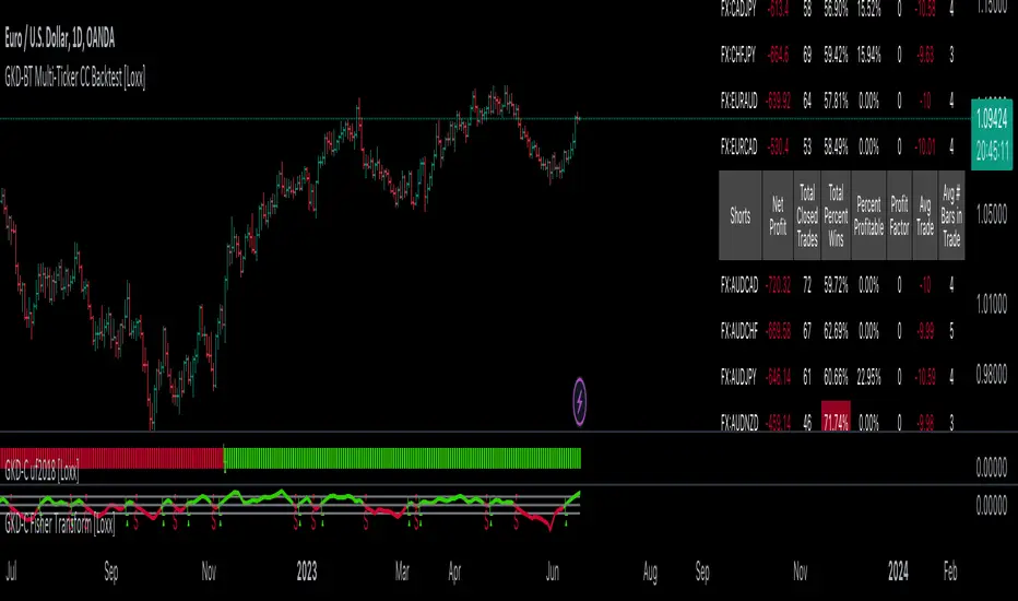
GKD-V Cercos Chaos vs Movement [Loxx]Giga Kaleidoscope GKD-V Cercos Chaos vs Movement is a Volatility/Volume module included in Loxx's "Giga Kaleidoscope Modularized Trading System".
█ GKD-V Cercos Chaos vs Movement
The following aims to provide a detailed explanation of Cercos Chaos vs Movement that helps traders determine market volatility by comparing two different measures: Buffer Move and Buffer Chaos. This indicator is non-directional and should be paired with a directional indicator to provide trading signals.
The first step in the process is defining a custom function that implements a variant of the sigmoid function. This function has a parameter that allows the output to be limited to the range of if desired. The sigmoid function will later be used to normalize the Buffer Chaos value.
Next, several input parameters are introduced, which can be adjusted by the user. These parameters include the period, chaos strength, chaos width, and movement strength. These values are essential to customizing the behavior of the indicator and adapting it to different market conditions and trading styles.
The wicks of the candles in the given time series are then calculated by subtracting the absolute difference between the open and close prices from the difference between the high and low prices. This step is crucial in determining the level of volatility in the market.
Subsequently, the highest high and lowest low over the defined period are identified by examining the maximum and minimum values of the open and close prices. This information is essential for calculating the total movement in the market over the period being analyzed.
Once the highest high and lowest low are found, the Buffer Move and Buffer Chaos values are calculated. The Buffer Move is the sum of the differences between the high and low prices for each candle in the period. This measure helps to identify the overall price movement in the market during the period.
On the other hand, the Buffer Chaos represents the sum of the wicks' lengths for each candle in the period. This measure is used to identify the level of uncertainty and disorder in the market during the period.
In the next step, the total movement in the market is calculated by subtracting the lowest low from the highest high. This value is then used to normalize the Buffer Move and Buffer Chaos values, ensuring they are on a comparable scale.
A comparison is made between the normalized Buffer Move and Buffer Chaos values. If the Buffer Move value is greater than the Buffer Chaos value, it indicates that there is enough volatility in the market to trade long or short. In such a case, the indicator suggests that the market conditions are favorable for trading. However, as this indicator is non-directional, a directional indicator should be used in conjunction with it to provide trading signals.
In conclusion, this custom trading indicator provides valuable insights into market volatility by comparing the Buffer Move and Buffer Chaos values. By offering a non-directional perspective, traders can use this indicator to gauge the potential for profitable trades and make informed decisions by pairing it with a directional indicator.
Additional Features
This indicator allows you to select from 33 source types. They are as follows:
Close
Open
High
Low
Median
Typical
Weighted
Average
Average Median Body
Trend Biased
Trend Biased (Extreme)
HA Close
HA Open
HA High
HA Low
HA Median
HA Typical
HA Weighted
HA Average
HA Average Median Body
HA Trend Biased
HA Trend Biased (Extreme)
HAB Close
HAB Open
HAB High
HAB Low
HAB Median
HAB Typical
HAB Weighted
HAB Average
HAB Average Median Body
HAB Trend Biased
HAB Trend Biased (Extreme)
What are Heiken Ashi "better" candles?
Heiken Ashi "better" candles are a modified version of the standard Heiken Ashi candles, which are a popular charting technique used in technical analysis. Heiken Ashi candles help traders identify trends and potential reversal points by smoothing out price data and reducing market noise. The "better formula" was proposed by Sebastian Schmidt in an article published by BNP Paribas in Warrants & Zertifikate, a German magazine, in August 2004. The aim of this formula is to further improve the smoothing of the Heiken Ashi chart and enhance its effectiveness in identifying trends and reversals.
Standard Heiken Ashi candles are calculated using the following formulas:
Heiken Ashi Close = (Open + High + Low + Close) / 4
Heiken Ashi Open = (Previous Heiken Ashi Open + Previous Heiken Ashi Close) / 2
Heiken Ashi High = Max (High, Heiken Ashi Open, Heiken Ashi Close)
Heiken Ashi Low = Min (Low, Heiken Ashi Open, Heiken Ashi Close)
The "better formula" modifies the standard Heiken Ashi calculation by incorporating additional smoothing, which can help reduce noise and make it easier to identify trends and reversals. The modified formulas for Heiken Ashi "better" candles are as follows:
Better Heiken Ashi Close = (Open + High + Low + Close) / 4
Better Heiken Ashi Open = (Previous Better Heiken Ashi Open + Previous Better Heiken Ashi Close) / 2
Better Heiken Ashi High = Max (High, Better Heiken Ashi Open, Better Heiken Ashi Close)
Better Heiken Ashi Low = Min (Low, Better Heiken Ashi Open, Better Heiken Ashi Close)
Smoothing Factor = 2 / (N + 1), where N is the chosen period for smoothing
Smoothed Better Heiken Ashi Open = (Better Heiken Ashi Open * Smoothing Factor) + (Previous Smoothed Better Heiken Ashi Open * (1 - Smoothing Factor))
Smoothed Better Heiken Ashi Close = (Better Heiken Ashi Close * Smoothing Factor) + (Previous Smoothed Better Heiken Ashi Close * (1 - Smoothing Factor))
The smoothed Better Heiken Ashi Open and Close values are then used to calculate the smoothed Better Heiken Ashi High and Low values, resulting in "better" candles that provide a clearer representation of the market trend and potential reversal points.
It's important to note that, like any other technical analysis tool, Heiken Ashi "better" candles are not foolproof and should be used in conjunction with other indicators and analysis techniques to make well-informed trading decisions.
Heiken Ashi "better" candles, as mentioned previously, provide a clearer representation of market trends and potential reversal points by reducing noise and smoothing out price data. When using these candles in conjunction with other technical analysis tools and indicators, traders can gain valuable insights into market behavior and make more informed decisions.
To effectively use Heiken Ashi "better" candles in your trading strategy, consider the following tips:
Trend Identification: Heiken Ashi "better" candles can help you identify the prevailing trend in the market. When the majority of the candles are green (or another color, depending on your chart settings) and there are no or few lower wicks, it may indicate a strong uptrend. Conversely, when the majority of the candles are red (or another color) and there are no or few upper wicks, it may signal a strong downtrend.
Trend Reversals: Look for potential trend reversals when a change in the color of the candles occurs, especially when accompanied by longer wicks. For example, if a green candle with a long lower wick is followed by a red candle, it could indicate a bearish reversal. Similarly, a red candle with a long upper wick followed by a green candle may suggest a bullish reversal.
Support and Resistance: You can use Heiken Ashi "better" candles to identify potential support and resistance levels. When the candles are consistently moving in one direction and then suddenly change color with longer wicks, it could indicate the presence of a support or resistance level.
Stop-Loss and Take-Profit: Using Heiken Ashi "better" candles can help you manage risk by determining optimal stop-loss and take-profit levels. For instance, you can place your stop-loss below the low of the most recent green candle in an uptrend or above the high of the most recent red candle in a downtrend.
Confirming Signals: Heiken Ashi "better" candles should be used in conjunction with other technical indicators, such as moving averages, oscillators, or chart patterns, to confirm signals and improve the accuracy of your analysis.
In this implementation, you have the choice of AMA, KAMA, or T3 smoothing. These are as follows:
Kaufman Adaptive Moving Average (KAMA)
The Kaufman Adaptive Moving Average (KAMA) is a type of adaptive moving average used in technical analysis to smooth out price fluctuations and identify trends. The KAMA adjusts its smoothing factor based on the market's volatility, making it more responsive in volatile markets and smoother in calm markets. The KAMA is calculated using three different efficiency ratios that determine the appropriate smoothing factor for the current market conditions. These ratios are based on the noise level of the market, the speed at which the market is moving, and the length of the moving average. The KAMA is a popular choice among traders who prefer to use adaptive indicators to identify trends and potential reversals.
Adaptive Moving Average
The Adaptive Moving Average (AMA) is a type of moving average that adjusts its sensitivity to price movements based on market conditions. It uses a ratio between the current price and the highest and lowest prices over a certain lookback period to determine its level of smoothing. The AMA can help reduce lag and increase responsiveness to changes in trend direction, making it useful for traders who want to follow trends while avoiding false signals. The AMA is calculated by multiplying a smoothing constant with the difference between the current price and the previous AMA value, then adding the result to the previous AMA value.
T3
The T3 moving average is a type of technical indicator used in financial analysis to identify trends in price movements. It is similar to the Exponential Moving Average (EMA) and the Double Exponential Moving Average (DEMA), but uses a different smoothing algorithm.
The T3 moving average is calculated using a series of exponential moving averages that are designed to filter out noise and smooth the data. The resulting smoothed data is then weighted with a non-linear function to produce a final output that is more responsive to changes in trend direction.
The T3 moving average can be customized by adjusting the length of the moving average, as well as the weighting function used to smooth the data. It is commonly used in conjunction with other technical indicators as part of a larger trading strategy.
█ Giga Kaleidoscope Modularized Trading System
Core components of an NNFX algorithmic trading strategy
The NNFX algorithm is built on the principles of trend, momentum, and volatility. There are six core components in the NNFX trading algorithm:
1. Volatility - price volatility; e.g., Average True Range, True Range Double, Close-to-Close, etc.
2. Baseline - a moving average to identify price trend
3. Confirmation 1 - a technical indicator used to identify trends
4. Confirmation 2 - a technical indicator used to identify trends
5. Continuation - a technical indicator used to identify trends
6. Volatility/Volume - a technical indicator used to identify volatility/volume breakouts/breakdown
7. Exit - a technical indicator used to determine when a trend is exhausted
What is Volatility in the NNFX trading system?
In the NNFX (No Nonsense Forex) trading system, ATR (Average True Range) is typically used to measure the volatility of an asset. It is used as a part of the system to help determine the appropriate stop loss and take profit levels for a trade. ATR is calculated by taking the average of the true range values over a specified period.
True range is calculated as the maximum of the following values:
-Current high minus the current low
-Absolute value of the current high minus the previous close
-Absolute value of the current low minus the previous close
ATR is a dynamic indicator that changes with changes in volatility. As volatility increases, the value of ATR increases, and as volatility decreases, the value of ATR decreases. By using ATR in NNFX system, traders can adjust their stop loss and take profit levels according to the volatility of the asset being traded. This helps to ensure that the trade is given enough room to move, while also minimizing potential losses.
Other types of volatility include True Range Double (TRD), Close-to-Close, and Garman-Klass
What is a Baseline indicator?
The baseline is essentially a moving average, and is used to determine the overall direction of the market.
The baseline in the NNFX system is used to filter out trades that are not in line with the long-term trend of the market. The baseline is plotted on the chart along with other indicators, such as the Moving Average (MA), the Relative Strength Index (RSI), and the Average True Range (ATR).
Trades are only taken when the price is in the same direction as the baseline. For example, if the baseline is sloping upwards, only long trades are taken, and if the baseline is sloping downwards, only short trades are taken. This approach helps to ensure that trades are in line with the overall trend of the market, and reduces the risk of entering trades that are likely to fail.
By using a baseline in the NNFX system, traders can have a clear reference point for determining the overall trend of the market, and can make more informed trading decisions. The baseline helps to filter out noise and false signals, and ensures that trades are taken in the direction of the long-term trend.
What is a Confirmation indicator?
Confirmation indicators are technical indicators that are used to confirm the signals generated by primary indicators. Primary indicators are the core indicators used in the NNFX system, such as the Average True Range (ATR), the Moving Average (MA), and the Relative Strength Index (RSI).
The purpose of the confirmation indicators is to reduce false signals and improve the accuracy of the trading system. They are designed to confirm the signals generated by the primary indicators by providing additional information about the strength and direction of the trend.
Some examples of confirmation indicators that may be used in the NNFX system include the Bollinger Bands, the MACD (Moving Average Convergence Divergence), and the MACD Oscillator. These indicators can provide information about the volatility, momentum, and trend strength of the market, and can be used to confirm the signals generated by the primary indicators.
In the NNFX system, confirmation indicators are used in combination with primary indicators and other filters to create a trading system that is robust and reliable. By using multiple indicators to confirm trading signals, the system aims to reduce the risk of false signals and improve the overall profitability of the trades.
What is a Continuation indicator?
In the NNFX (No Nonsense Forex) trading system, a continuation indicator is a technical indicator that is used to confirm a current trend and predict that the trend is likely to continue in the same direction. A continuation indicator is typically used in conjunction with other indicators in the system, such as a baseline indicator, to provide a comprehensive trading strategy.
What is a Volatility/Volume indicator?
Volume indicators, such as the On Balance Volume (OBV), the Chaikin Money Flow (CMF), or the Volume Price Trend (VPT), are used to measure the amount of buying and selling activity in a market. They are based on the trading volume of the market, and can provide information about the strength of the trend. In the NNFX system, volume indicators are used to confirm trading signals generated by the Moving Average and the Relative Strength Index. Volatility indicators include Average Direction Index, Waddah Attar, and Volatility Ratio. In the NNFX trading system, volatility is a proxy for volume and vice versa.
By using volume indicators as confirmation tools, the NNFX trading system aims to reduce the risk of false signals and improve the overall profitability of trades. These indicators can provide additional information about the market that is not captured by the primary indicators, and can help traders to make more informed trading decisions. In addition, volume indicators can be used to identify potential changes in market trends and to confirm the strength of price movements.
What is an Exit indicator?
The exit indicator is used in conjunction with other indicators in the system, such as the Moving Average (MA), the Relative Strength Index (RSI), and the Average True Range (ATR), to provide a comprehensive trading strategy.
The exit indicator in the NNFX system can be any technical indicator that is deemed effective at identifying optimal exit points. Examples of exit indicators that are commonly used include the Parabolic SAR, the Average Directional Index (ADX), and the Chandelier Exit.
The purpose of the exit indicator is to identify when a trend is likely to reverse or when the market conditions have changed, signaling the need to exit a trade. By using an exit indicator, traders can manage their risk and prevent significant losses.
In the NNFX system, the exit indicator is used in conjunction with a stop loss and a take profit order to maximize profits and minimize losses. The stop loss order is used to limit the amount of loss that can be incurred if the trade goes against the trader, while the take profit order is used to lock in profits when the trade is moving in the trader's favor.
Overall, the use of an exit indicator in the NNFX trading system is an important component of a comprehensive trading strategy. It allows traders to manage their risk effectively and improve the profitability of their trades by exiting at the right time.
How does Loxx's GKD (Giga Kaleidoscope Modularized Trading System) implement the NNFX algorithm outlined above?
Loxx's GKD v1.0 system has five types of modules (indicators/strategies). These modules are:
1. GKD-BT - Backtesting module (Volatility, Number 1 in the NNFX algorithm)
2. GKD-B - Baseline module (Baseline and Volatility/Volume, Numbers 1 and 2 in the NNFX algorithm)
3. GKD-C - Confirmation 1/2 and Continuation module (Confirmation 1/2 and Continuation, Numbers 3, 4, and 5 in the NNFX algorithm)
4. GKD-V - Volatility/Volume module (Confirmation 1/2, Number 6 in the NNFX algorithm)
5. GKD-E - Exit module (Exit, Number 7 in the NNFX algorithm)
(additional module types will added in future releases)
Each module interacts with every module by passing data between modules. Data is passed between each module as described below:
GKD-B => GKD-V => GKD-C(1) => GKD-C(2) => GKD-C(Continuation) => GKD-E => GKD-BT
That is, the Baseline indicator passes its data to Volatility/Volume. The Volatility/Volume indicator passes its values to the Confirmation 1 indicator. The Confirmation 1 indicator passes its values to the Confirmation 2 indicator. The Confirmation 2 indicator passes its values to the Continuation indicator. The Continuation indicator passes its values to the Exit indicator, and finally, the Exit indicator passes its values to the Backtest strategy.
This chaining of indicators requires that each module conform to Loxx's GKD protocol, therefore allowing for the testing of every possible combination of technical indicators that make up the six components of the NNFX algorithm.
What does the application of the GKD trading system look like?
Example trading system:
Backtest: Strategy with 1-3 take profits, trailing stop loss, multiple types of PnL volatility, and 2 backtesting styles
Baseline: Hull Moving Average
Volatility/Volume: Cercos Chaos vs Movement as shown on the chart above
Confirmation 1: Fisher Transform
Confirmation 2: Williams Percent Range
Continuation: Cercos Chaos vs Movement
Exit: Rex Oscillator
Each GKD indicator is denoted with a module identifier of either: GKD-BT, GKD-B, GKD-C, GKD-V, or GKD-E. This allows traders to understand to which module each indicator belongs and where each indicator fits into the GKD protocol chain.
Giga Kaleidoscope Modularized Trading System Signals (based on the NNFX algorithm)
Standard Entry
1. GKD-C Confirmation 1 Signal
2. GKD-B Baseline agrees
3. Price is within a range of 0.2x Volatility and 1.0x Volatility of the Goldie Locks Mean
4. GKD-C Confirmation 2 agrees
5. GKD-V Volatility/Volume agrees
Baseline Entry
1. GKD-B Baseline signal
2. GKD-C Confirmation 1 agrees
3. Price is within a range of 0.2x Volatility and 1.0x Volatility of the Goldie Locks Mean
4. GKD-C Confirmation 2 agrees
5. GKD-V Volatility/Volume agrees
6. GKD-C Confirmation 1 signal was less than 7 candles prior
Volatility/Volume Entry
1. GKD-V Volatility/Volume signal
2. GKD-C Confirmation 1 agrees
3. Price is within a range of 0.2x Volatility and 1.0x Volatility of the Goldie Locks Mean
4. GKD-C Confirmation 2 agrees
5. GKD-B Baseline agrees
6. GKD-C Confirmation 1 signal was less than 7 candles prior
Continuation Entry
1. Standard Entry, Baseline Entry, or Pullback; entry triggered previously
2. GKD-B Baseline hasn't crossed since entry signal trigger
3. GKD-C Confirmation Continuation Indicator signals
4. GKD-C Confirmation 1 agrees
5. GKD-B Baseline agrees
6. GKD-C Confirmation 2 agrees
1-Candle Rule Standard Entry
1. GKD-C Confirmation 1 signal
2. GKD-B Baseline agrees
3. Price is within a range of 0.2x Volatility and 1.0x Volatility of the Goldie Locks Mean
Next Candle:
1. Price retraced (Long: close < close or Short: close > close )
2. GKD-B Baseline agrees
3. GKD-C Confirmation 1 agrees
4. GKD-C Confirmation 2 agrees
5. GKD-V Volatility/Volume agrees
1-Candle Rule Baseline Entry
1. GKD-B Baseline signal
2. GKD-C Confirmation 1 agrees
3. Price is within a range of 0.2x Volatility and 1.0x Volatility of the Goldie Locks Mean
4. GKD-C Confirmation 1 signal was less than 7 candles prior
Next Candle:
1. Price retraced (Long: close < close or Short: close > close )
2. GKD-B Baseline agrees
3. GKD-C Confirmation 1 agrees
4. GKD-C Confirmation 2 agrees
5. GKD-V Volatility/Volume Agrees
1-Candle Rule Volatility/Volume Entry
1. GKD-V Volatility/Volume signal
2. GKD-C Confirmation 1 agrees
3. Price is within a range of 0.2x Volatility and 1.0x Volatility of the Goldie Locks Mean
4. GKD-C Confirmation 1 signal was less than 7 candles prior
Next Candle:
1. Price retraced (Long: close < close or Short: close > close)
2. GKD-B Volatility/Volume agrees
3. GKD-C Confirmation 1 agrees
4. GKD-C Confirmation 2 agrees
5. GKD-B Baseline agrees
PullBack Entry
1. GKD-B Baseline signal
2. GKD-C Confirmation 1 agrees
3. Price is beyond 1.0x Volatility of Baseline
Next Candle:
1. Price is within a range of 0.2x Volatility and 1.0x Volatility of the Goldie Locks Mean
2. GKD-C Confirmation 1 agrees
3. GKD-C Confirmation 2 agrees
4. GKD-V Volatility/Volume Agrees
]█ Setting up the GKD
The GKD system involves chaining indicators together. These are the steps to set this up.
Use a GKD-C indicator alone on a chart
1. Inside the GKD-C indicator, change the "Confirmation Type" setting to "Solo Confirmation Simple"
Use a GKD-V indicator alone on a chart
**nothing, it's already useable on the chart without any settings changes
Use a GKD-B indicator alone on a chart
**nothing, it's already useable on the chart without any settings changes
Baseline (Baseline, Backtest)
1. Import the GKD-B Baseline into the GKD-BT Backtest: "Input into Volatility/Volume or Backtest (Baseline testing)"
2. Inside the GKD-BT Backtest, change the setting "Backtest Special" to "Baseline"
Volatility/Volume (Volatility/Volume, Backte st)
1. Inside the GKD-V indicator, change the "Testing Type" setting to "Solo"
2. Inside the GKD-V indicator, change the "Signal Type" setting to "Crossing" (neither traditional nor both can be backtested)
3. Import the GKD-V indicator into the GKD-BT Backtest: "Input into C1 or Backtest"
4. Inside the GKD-BT Backtest, change the setting "Backtest Special" to "Volatility/Volume"
5. Inside the GKD-BT Backtest, a) change the setting "Backtest Type" to "Trading" if using a directional GKD-V indicator; or, b) change the setting "Backtest Type" to "Full" if using a directional or non-directional GKD-V indicator (non-directional GKD-V can only test Longs and Shorts separately)
6. If "Backtest Type" is set to "Full": Inside the GKD-BT Backtest, change the setting "Backtest Side" to "Long" or "Short
7. If "Backtest Type" is set to "Full": To allow the system to open multiple orders at one time so you test all Longs or Shorts, open the GKD-BT Backtest, click the tab "Properties" and then insert a value of something like 10 orders into the "Pyramiding" settings. This will allow 10 orders to be opened at one time which should be enough to catch all possible Longs or Shorts.
Solo Confirmation Simple (Confirmation, Backtest)
1. Inside the GKD-C indicator, change the "Confirmation Type" setting to "Solo Confirmation Simple"
1. Import the GKD-C indicator into the GKD-BT Backtest: "Input into Backtest"
2. Inside the GKD-BT Backtest, change the setting "Backtest Special" to "Solo Confirmation Simple"
Solo Confirmation Complex without Exits (Baseline, Volatility/Volume, Confirmation, Backtest)
1. Inside the GKD-V indicator, change the "Testing Type" setting to "Chained"
2. Import the GKD-B Baseline into the GKD-V indicator: "Input into Volatility/Volume or Backtest (Baseline testing)"
3. Inside the GKD-C indicator, change the "Confirmation Type" setting to "Solo Confirmation Complex"
4. Import the GKD-V indicator into the GKD-C indicator: "Input into C1 or Backtest"
5. Inside the GKD-BT Backtest, change the setting "Backtest Special" to "GKD Full wo/ Exits"
6. Import the GKD-C into the GKD-BT Backtest: "Input into Exit or Backtest"
Solo Confirmation Complex with Exits (Baseline, Volatility/Volume, Confirmation, Exit, Backtest)
1. Inside the GKD-V indicator, change the "Testing Type" setting to "Chained"
2. Import the GKD-B Baseline into the GKD-V indicator: "Input into Volatility/Volume or Backtest (Baseline testing)"
3. Inside the GKD-C indicator, change the "Confirmation Type" setting to "Solo Confirmation Complex"
4. Import the GKD-V indicator into the GKD-C indicator: "Input into C1 or Backtest"
5. Import the GKD-C indicator into the GKD-E indicator: "Input into Exit"
6. Inside the GKD-BT Backtest, change the setting "Backtest Special" to "GKD Full w/ Exits"
7. Import the GKD-E into the GKD-BT Backtest: "Input into Backtest"
Full GKD without Exits (Baseline, Volatility/Volume, Confirmation 1, Confirmation 2, Continuation, Backtest)
1. Inside the GKD-V indicator, change the "Testing Type" setting to "Chained"
2. Import the GKD-B Baseline into the GKD-V indicator: "Input into Volatility/Volume or Backtest (Baseline testing)"
3. Inside the GKD-C 1 indicator, change the "Confirmation Type" setting to "Confirmation 1"
4. Import the GKD-V indicator into the GKD-C 1 indicator: "Input into C1 or Backtest"
5. Inside the GKD-C 2 indicator, change the "Confirmation Type" setting to "Confirmation 2"
6. Import the GKD-C 1 indicator into the GKD-C 2 indicator: "Input into C2"
7. Inside the GKD-C Continuation indicator, change the "Confirmation Type" setting to "Continuation"
8. Inside the GKD-BT Backtest, change the setting "Backtest Special" to "GKD Full wo/ Exits"
9. Import the GKD-E into the GKD-BT Backtest: "Input into Exit or Backtest"
Full GKD with Exits (Baseline, Volatility/Volume, Confirmation 1, Confirmation 2, Continuation, Exit, Backtest)
1. Inside the GKD-V indicator, change the "Testing Type" setting to "Chained"
2. Import the GKD-B Baseline into the GKD-V indicator: "Input into Volatility/Volume or Backtest (Baseline testing)"
3. Inside the GKD-C 1 indicator, change the "Confirmation Type" setting to "Confirmation 1"
4. Import the GKD-V indicator into the GKD-C 1 indicator: "Input into C1 or Backtest"
5. Inside the GKD-C 2 indicator, change the "Confirmation Type" setting to "Confirmation 2"
6. Import the GKD-C 1 indicator into the GKD-C 2 indicator: "Input into C2"
7. Inside the GKD-C Continuation indicator, change the "Confirmation Type" setting to "Continuation"
8. Import the GKD-C Continuation indicator into the GKD-E indicator: "Input into Exit"
9. Inside the GKD-BT Backtest, change the setting "Backtest Special" to "GKD Full w/ Exits"
10. Import the GKD-E into the GKD-BT Backtest: "Input into Backtest"
Baseline + Volatility/Volume (Baseline, Volatility/Volume, Backtest)
1. Inside the GKD-V indicator, change the "Testing Type" setting to "Baseline + Volatility/Volume"
2. Inside the GKD-V indicator, make sure the "Signal Type" setting is set to "Traditional"
3. Import the GKD-B Baseline into the GKD-V indicator: "Input into Volatility/Volume or Backtest (Baseline testing)"
4. Inside the GKD-BT Backtest, change the setting "Backtest Special" to "Baseline + Volatility/Volume"
5. Import the GKD-V into the GKD-BT Backtest: "Input into C1 or Backtest"
6. Inside the GKD-BT Backtest, change the setting "Backtest Type" to "Full". For this backtest, you must test Longs and Shorts separately
7. To allow the system to open multiple orders at one time so you can test all Longs or Shorts, open the GKD-BT Backtest, click the tab "Properties" and then insert a value of something like 10 orders into the "Pyramiding" settings. This will allow 10 orders to be opened at one time which should be enough to catch all possible Longs or Shorts.
Requirements
Inputs
Chained: GKD-B Baseline
Solo: NA, no inputs
Baseline + Volatility/Volume: GKD-B Baseline
Outputs
Chained: GKD-C indicators Confirmation 1 or Solo Confirmation Complex
Solo: GKD-BT Backtest
Baseline + Volatility/Volume: GKD-BT Backtest
Additional features will be added in future releases.

GKD-C Juirk-Filtered QQE Histogram [Loxx]Giga Kaleidoscope GKD-C Juirk-Filtered QQE Histogram is a Confirmation module included in Loxx's "Giga Kaleidoscope Modularized Trading System".
█ Giga Kaleidoscope Modularized Trading System
What is Loxx's "Giga Kaleidoscope Modularized Trading System"?
The Giga Kaleidoscope Modularized Trading System is a trading system built on the philosophy of the NNFX (No Nonsense Forex) algorithmic trading.
What is the NNFX algorithmic trading strategy?
The NNFX (No-Nonsense Forex) trading system is a comprehensive approach to Forex trading that is designed to simplify the process and remove the confusion and complexity that often surrounds trading. The system was developed by a Forex trader who goes by the pseudonym "VP" and has gained a significant following in the Forex community.
The NNFX trading system is based on a set of rules and guidelines that help traders make objective and informed decisions. These rules cover all aspects of trading, including market analysis, trade entry, stop loss placement, and trade management.
Here are the main components of the NNFX trading system:
1. Trading Philosophy: The NNFX trading system is based on the idea that successful trading requires a comprehensive understanding of the market, objective analysis, and strict risk management. The system aims to remove subjective elements from trading and focuses on objective rules and guidelines.
2. Technical Analysis: The NNFX trading system relies heavily on technical analysis and uses a range of indicators to identify high-probability trading opportunities. The system uses a combination of trend-following and mean-reverting strategies to identify trades.
3. Market Structure: The NNFX trading system emphasizes the importance of understanding the market structure, including price action, support and resistance levels, and market cycles. The system uses a range of tools to identify the market structure, including trend lines, channels, and moving averages.
4. Trade Entry: The NNFX trading system has strict rules for trade entry. The system uses a combination of technical indicators to identify high-probability trades, and traders must meet specific criteria to enter a trade.
5. Stop Loss Placement: The NNFX trading system places a significant emphasis on risk management and requires traders to place a stop loss order on every trade. The system uses a combination of technical analysis and market structure to determine the appropriate stop loss level.
6. Trade Management: The NNFX trading system has specific rules for managing open trades. The system aims to minimize risk and maximize profit by using a combination of trailing stops, take profit levels, and position sizing.
Overall, the NNFX trading system is designed to be a straightforward and easy-to-follow approach to Forex trading that can be applied by traders of all skill levels.
Core components of an NNFX algorithmic trading strategy
The NNFX algorithm is built on the principles of trend, momentum, and volatility. There are six core components in the NNFX trading algorithm:
1. Volatility - price volatility; e.g., Average True Range, True Range Double, Close-to-Close, etc.
2. Baseline - a moving average to identify price trend
3. Confirmation 1 - a technical indicator used to identify trends
4. Confirmation 2 - a technical indicator used to identify trends
5. Continuation - a technical indicator used to identify trends
6. Volatility/Volume - a technical indicator used to identify volatility/volume breakouts/breakdown
7. Exit - a technical indicator used to determine when a trend is exhausted
What is Volatility in the NNFX trading system?
In the NNFX (No Nonsense Forex) trading system, ATR (Average True Range) is typically used to measure the volatility of an asset. It is used as a part of the system to help determine the appropriate stop loss and take profit levels for a trade. ATR is calculated by taking the average of the true range values over a specified period.
True range is calculated as the maximum of the following values:
-Current high minus the current low
-Absolute value of the current high minus the previous close
-Absolute value of the current low minus the previous close
ATR is a dynamic indicator that changes with changes in volatility. As volatility increases, the value of ATR increases, and as volatility decreases, the value of ATR decreases. By using ATR in NNFX system, traders can adjust their stop loss and take profit levels according to the volatility of the asset being traded. This helps to ensure that the trade is given enough room to move, while also minimizing potential losses.
Other types of volatility include True Range Double (TRD), Close-to-Close, and Garman-Klass
What is a Baseline indicator?
The baseline is essentially a moving average, and is used to determine the overall direction of the market.
The baseline in the NNFX system is used to filter out trades that are not in line with the long-term trend of the market. The baseline is plotted on the chart along with other indicators, such as the Moving Average (MA), the Relative Strength Index (RSI), and the Average True Range (ATR).
Trades are only taken when the price is in the same direction as the baseline. For example, if the baseline is sloping upwards, only long trades are taken, and if the baseline is sloping downwards, only short trades are taken. This approach helps to ensure that trades are in line with the overall trend of the market, and reduces the risk of entering trades that are likely to fail.
By using a baseline in the NNFX system, traders can have a clear reference point for determining the overall trend of the market, and can make more informed trading decisions. The baseline helps to filter out noise and false signals, and ensures that trades are taken in the direction of the long-term trend.
What is a Confirmation indicator?
Confirmation indicators are technical indicators that are used to confirm the signals generated by primary indicators. Primary indicators are the core indicators used in the NNFX system, such as the Average True Range (ATR), the Moving Average (MA), and the Relative Strength Index (RSI).
The purpose of the confirmation indicators is to reduce false signals and improve the accuracy of the trading system. They are designed to confirm the signals generated by the primary indicators by providing additional information about the strength and direction of the trend.
Some examples of confirmation indicators that may be used in the NNFX system include the Bollinger Bands, the MACD (Moving Average Convergence Divergence), and the MACD Oscillator. These indicators can provide information about the volatility, momentum, and trend strength of the market, and can be used to confirm the signals generated by the primary indicators.
In the NNFX system, confirmation indicators are used in combination with primary indicators and other filters to create a trading system that is robust and reliable. By using multiple indicators to confirm trading signals, the system aims to reduce the risk of false signals and improve the overall profitability of the trades.
What is a Continuation indicator?
In the NNFX (No Nonsense Forex) trading system, a continuation indicator is a technical indicator that is used to confirm a current trend and predict that the trend is likely to continue in the same direction. A continuation indicator is typically used in conjunction with other indicators in the system, such as a baseline indicator, to provide a comprehensive trading strategy.
What is a Volatility/Volume indicator?
Volume indicators, such as the On Balance Volume (OBV), the Chaikin Money Flow (CMF), or the Volume Price Trend (VPT), are used to measure the amount of buying and selling activity in a market. They are based on the trading volume of the market, and can provide information about the strength of the trend. In the NNFX system, volume indicators are used to confirm trading signals generated by the Moving Average and the Relative Strength Index. Volatility indicators include Average Direction Index, Waddah Attar, and Volatility Ratio. In the NNFX trading system, volatility is a proxy for volume and vice versa.
By using volume indicators as confirmation tools, the NNFX trading system aims to reduce the risk of false signals and improve the overall profitability of trades. These indicators can provide additional information about the market that is not captured by the primary indicators, and can help traders to make more informed trading decisions. In addition, volume indicators can be used to identify potential changes in market trends and to confirm the strength of price movements.
What is an Exit indicator?
The exit indicator is used in conjunction with other indicators in the system, such as the Moving Average (MA), the Relative Strength Index (RSI), and the Average True Range (ATR), to provide a comprehensive trading strategy.
The exit indicator in the NNFX system can be any technical indicator that is deemed effective at identifying optimal exit points. Examples of exit indicators that are commonly used include the Parabolic SAR, the Average Directional Index (ADX), and the Chandelier Exit.
The purpose of the exit indicator is to identify when a trend is likely to reverse or when the market conditions have changed, signaling the need to exit a trade. By using an exit indicator, traders can manage their risk and prevent significant losses.
In the NNFX system, the exit indicator is used in conjunction with a stop loss and a take profit order to maximize profits and minimize losses. The stop loss order is used to limit the amount of loss that can be incurred if the trade goes against the trader, while the take profit order is used to lock in profits when the trade is moving in the trader's favor.
Overall, the use of an exit indicator in the NNFX trading system is an important component of a comprehensive trading strategy. It allows traders to manage their risk effectively and improve the profitability of their trades by exiting at the right time.
How does Loxx's GKD (Giga Kaleidoscope Modularized Trading System) implement the NNFX algorithm outlined above?
Loxx's GKD v1.0 system has five types of modules (indicators/strategies). These modules are:
1. GKD-BT - Backtesting module (Volatility, Number 1 in the NNFX algorithm)
2. GKD-B - Baseline module (Baseline and Volatility/Volume, Numbers 1 and 2 in the NNFX algorithm)
3. GKD-C - Confirmation 1/2 and Continuation module (Confirmation 1/2 and Continuation, Numbers 3, 4, and 5 in the NNFX algorithm)
4. GKD-V - Volatility/Volume module (Confirmation 1/2, Number 6 in the NNFX algorithm)
5. GKD-E - Exit module (Exit, Number 7 in the NNFX algorithm)
(additional module types will added in future releases)
Each module interacts with every module by passing data between modules. Data is passed between each module as described below:
GKD-B => GKD-V => GKD-C(1) => GKD-C(2) => GKD-C(Continuation) => GKD-E => GKD-BT
That is, the Baseline indicator passes its data to Volatility/Volume. The Volatility/Volume indicator passes its values to the Confirmation 1 indicator. The Confirmation 1 indicator passes its values to the Confirmation 2 indicator. The Confirmation 2 indicator passes its values to the Continuation indicator. The Continuation indicator passes its values to the Exit indicator, and finally, the Exit indicator passes its values to the Backtest strategy.
This chaining of indicators requires that each module conform to Loxx's GKD protocol, therefore allowing for the testing of every possible combination of technical indicators that make up the six components of the NNFX algorithm.
What does the application of the GKD trading system look like?
Example trading system:
Backtest: Strategy with 1-3 take profits, trailing stop loss, multiple types of PnL volatility, and 2 backtesting styles
Baseline: Hull Moving Average
Volatility/Volume: Hurst Exponent
Confirmation 1: Juirk-Filtered QQE Histogram as shown on the chart above
Confirmation 2: Williams Percent Range
Continuation: Fisher Transform
Exit: Rex Oscillator
Each GKD indicator is denoted with a module identifier of either: GKD-BT, GKD-B, GKD-C, GKD-V, or GKD-E. This allows traders to understand to which module each indicator belongs and where each indicator fits into the GKD protocol chain.
Giga Kaleidoscope Modularized Trading System Signals (based on the NNFX algorithm)
Standard Entry
1. GKD-C Confirmation 1 Signal
2. GKD-B Baseline agrees
3. Price is within a range of 0.2x Volatility and 1.0x Volatility of the Goldie Locks Mean
4. GKD-C Confirmation 2 agrees
5. GKD-V Volatility/Volume agrees
Baseline Entry
1. GKD-B Baseline signal
2. GKD-C Confirmation 1 agrees
3. Price is within a range of 0.2x Volatility and 1.0x Volatility of the Goldie Locks Mean
4. GKD-C Confirmation 2 agrees
5. GKD-V Volatility/Volume agrees
6. GKD-C Confirmation 1 signal was less than 7 candles prior
Continuation Entry
1. Standard Entry, Baseline Entry, or Pullback; entry triggered previously
2. GKD-B Baseline hasn't crossed since entry signal trigger
3. GKD-C Confirmation Continuation Indicator signals
4. GKD-C Confirmation 1 agrees
5. GKD-B Baseline agrees
6. GKD-C Confirmation 2 agrees
1-Candle Rule Standard Entry
1. GKD-C Confirmation 1 signal
2. GKD-B Baseline agrees
3. Price is within a range of 0.2x Volatility and 1.0x Volatility of the Goldie Locks Mean
Next Candle:
1. Price retraced (Long: close < close or Short: close > close )
2. GKD-B Baseline agrees
3. GKD-C Confirmation 1 agrees
4. GKD-C Confirmation 2 agrees
5. GKD-V Volatility/Volume agrees
1-Candle Rule Baseline Entry
1. GKD-B Baseline signal
2. GKD-C Confirmation 1 agrees
3. Price is within a range of 0.2x Volatility and 1.0x Volatility of the Goldie Locks Mean
4. GKD-C Confirmation 1 signal was less than 7 candles prior
Next Candle:
1. Price retraced (Long: close < close or Short: close > close )
2. GKD-B Baseline agrees
3. GKD-C Confirmation 1 agrees
4. GKD-C Confirmation 2 agrees
5. GKD-V Volatility/Volume Agrees
PullBack Entry
1. GKD-B Baseline signal
2. GKD-C Confirmation 1 agrees
3. Price is beyond 1.0x Volatility of Baseline
Next Candle:
1. Price is within a range of 0.2x Volatility and 1.0x Volatility of the Goldie Locks Mean
3. GKD-C Confirmation 1 agrees
4. GKD-C Confirmation 2 agrees
5. GKD-V Volatility/Volume Agrees
█ GKD-C Juirk-Filtered QQE Histogram
What is Parabolic-Weighted Velocity?
Parabolic-Weighted Velocity (PWV) is a mathematical model used in sports science to estimate the velocity of an athlete during a given movement or exercise. This model uses a parabolic weighting function to give more importance to the velocities achieved in the middle of the movement and less importance to the velocities achieved at the beginning and end of the movement.
PWV takes into account the acceleration and deceleration of an athlete during the movement, and uses this information to calculate an average velocity. The model assumes that the athlete moves at a constant velocity during the middle portion of the movement and that the velocity increases and decreases smoothly at the beginning and end of the movement.
The parabolic weighting function used in PWV is based on the principle of impulse momentum, which states that the change in momentum of an object is equal to the impulse applied to it. The impulse is calculated as the force applied to an object multiplied by the time during which the force is applied. By giving more weight to the velocities achieved during the middle of the movement, PWV takes into account the impulse generated during this period of the movement.
PWV is commonly used in sports science to measure the performance of athletes during activities such as sprinting, jumping, and throwing. It is often used in conjunction with other metrics such as power and force to provide a comprehensive picture of an athlete's performance. Additionally, PWV can be used to compare the performance of different athletes or to track an athlete's progress over time.
Overall, Parabolic-Weighted Velocity is a useful tool in sports science for estimating an athlete's velocity during a movement or exercise, taking into account the acceleration and deceleration of the athlete during the movement.
What is QQE?
Quantitative Qualitative Estimation (QQE) is a technical analysis indicator used to identify trends and trading opportunities in financial markets. It is based on a combination of two popular technical analysis indicators - the Relative Strength Index (RSI) and Moving Averages (MA).
The QQE indicator uses a smoothed RSI to determine the trend direction, and a moving average of the smoothed RSI to identify potential trend changes. The indicator then plots a series of bands above and below the moving average to indicate overbought and oversold conditions in the market.
The QQE indicator is designed to provide traders with a reliable signal that confirms the strength of a trend or indicates a possible trend reversal. It is particularly useful for traders who are looking to trade in markets that are trending strongly, but also want to identify when a trend is losing momentum or reversing.
Traders can use QQE in a number of different ways, including as a confirmation tool for other indicators or as a standalone indicator. For example, when used in conjunction with other technical analysis tools like support and resistance levels, the QQE indicator can help traders identify key entry and exit points for their trades.
One of the main advantages of the QQE indicator is that it is designed to be more reliable than other indicators that can generate false signals. By smoothing out the price action, the QQE indicator can provide traders with more accurate and reliable signals, which can help them make more profitable trading decisions.
In conclusion, QQE is a popular technical analysis indicator that traders use to identify trends and trading opportunities in financial markets. It combines the RSI and moving average indicators and is designed to provide traders with reliable signals that confirm the strength of a trend or indicate a possible trend reversal.
What is the Jurik Filter?
The Jurik Filter is a technical analysis tool that is used to filter out market noise and identify trends in financial markets. It was developed by Mark Jurik in the 1990s and is based on a non-linear smoothing algorithm that provides a more accurate representation of price movements.
Traditional moving averages, such as the Simple Moving Average ( SMA ) or Exponential Moving Average ( EMA ), are linear filters that produce a lag between price and the moving average line. This can cause false signals during periods of market volatility , which can result in losses for traders and investors.
The Jurik Filter is designed to address this issue by incorporating a damping factor into the smoothing algorithm. This damping factor adjusts the filter's responsiveness to the changes in price, allowing it to filter out market noise without overshooting price peaks and valleys.
The Jurik Filter is calculated using a mathematical formula that takes into account the current and past prices of an asset, as well as the volatility of the market. This formula incorporates the damping factor and produces a smoother price curve than traditional moving average filters.
One of the advantages of the Jurik Filter is its ability to adjust to changing market conditions. The damping factor can be adjusted to suit different securities and time frames, making it a versatile tool for traders and investors.
Traders and investors often use the Jurik Filter in conjunction with other technical analysis tools, such as the MACD or RSI , to confirm or complement their trading strategies. By filtering out market noise and identifying trends in the financial markets, the Jurik Filter can help improve the accuracy of trading signals and reduce the risks of false signals during periods of market volatility .
Overall, the Jurik Filter is a powerful technical analysis tool that can help traders and investors make more informed decisions about buying and selling securities. By providing a smoother price curve and reducing false signals, it can help improve trading performance and reduce risk in volatile markets.
This indicator contains 7 different types of RSI:
RSX
Regular
Slow
Rapid
Harris
Cuttler
Ehlers Smoothed
What is RSI?
RSI stands for Relative Strength Index . It is a technical indicator used to measure the strength or weakness of a financial instrument's price action.
The RSI is calculated based on the price movement of an asset over a specified period of time, typically 14 days, and is expressed on a scale of 0 to 100. The RSI is considered overbought when it is above 70 and oversold when it is below 30.
Traders and investors use the RSI to identify potential buy and sell signals. When the RSI indicates that an asset is oversold, it may be considered a buying opportunity, while an overbought RSI may signal that it is time to sell or take profits.
It's important to note that the RSI should not be used in isolation and should be used in conjunction with other technical and fundamental analysis tools to make informed trading decisions.
What is RSX?
Jurik RSX is a technical analysis indicator that is a variation of the Relative Strength Index Smoothed ( RSX ) indicator. It was developed by Mark Jurik and is designed to help traders identify trends and momentum in the market.
The Jurik RSX uses a combination of the RSX indicator and an adaptive moving average (AMA) to smooth out the price data and reduce the number of false signals. The adaptive moving average is designed to adjust the smoothing period based on the current market conditions, which makes the indicator more responsive to changes in price.
The Jurik RSX can be used to identify potential trend reversals and momentum shifts in the market. It oscillates between 0 and 100, with values above 50 indicating a bullish trend and values below 50 indicating a bearish trend . Traders can use these levels to make trading decisions, such as buying when the indicator crosses above 50 and selling when it crosses below 50.
The Jurik RSX is a more advanced version of the RSX indicator, and while it can be useful in identifying potential trade opportunities, it should not be used in isolation. It is best used in conjunction with other technical and fundamental analysis tools to make informed trading decisions.
What is Slow RSI?
Slow RSI is a variation of the traditional Relative Strength Index ( RSI ) indicator. It is a more smoothed version of the RSI and is designed to filter out some of the noise and short-term price fluctuations that can occur with the standard RSI .
The Slow RSI uses a longer period of time than the traditional RSI , typically 21 periods instead of 14. This longer period helps to smooth out the price data and makes the indicator less reactive to short-term price fluctuations.
Like the traditional RSI , the Slow RSI is used to identify potential overbought and oversold conditions in the market. It oscillates between 0 and 100, with values above 70 indicating overbought conditions and values below 30 indicating oversold conditions. Traders often use these levels as potential buy and sell signals.
The Slow RSI is a more conservative version of the RSI and can be useful in identifying longer-term trends in the market. However, it can also be slower to respond to changes in price, which may result in missed trading opportunities. Traders may choose to use a combination of both the Slow RSI and the traditional RSI to make informed trading decisions.
What is Rapid RSI?
Same as regular RSI but with a faster calculation method
What is Harris RSI?
Harris RSI is a technical analysis indicator that is a variation of the Relative Strength Index ( RSI ). It was developed by Larry Harris and is designed to help traders identify potential trend changes and momentum shifts in the market.
The Harris RSI uses a different calculation formula compared to the traditional RSI . It takes into account both the opening and closing prices of a financial instrument, as well as the high and low prices. The Harris RSI is also normalized to a range of 0 to 100, with values above 50 indicating a bullish trend and values below 50 indicating a bearish trend .
Like the traditional RSI , the Harris RSI is used to identify potential overbought and oversold conditions in the market. It oscillates between 0 and 100, with values above 70 indicating overbought conditions and values below 30 indicating oversold conditions. Traders often use these levels as potential buy and sell signals.
The Harris RSI is a more advanced version of the RSI and can be useful in identifying longer-term trends in the market. However, it can also generate more false signals than the standard RSI . Traders may choose to use a combination of both the Harris RSI and the traditional RSI to make informed trading decisions.
What is Cuttler RSI?
Cuttler RSI is a technical analysis indicator that is a variation of the Relative Strength Index ( RSI ). It was developed by Curt Cuttler and is designed to help traders identify potential trend changes and momentum shifts in the market.
The Cuttler RSI uses a different calculation formula compared to the traditional RSI . It takes into account the difference between the closing price of a financial instrument and the average of the high and low prices over a specified period of time. This difference is then normalized to a range of 0 to 100, with values above 50 indicating a bullish trend and values below 50 indicating a bearish trend .
Like the traditional RSI , the Cuttler RSI is used to identify potential overbought and oversold conditions in the market. It oscillates between 0 and 100, with values above 70 indicating overbought conditions and values below 30 indicating oversold conditions. Traders often use these levels as potential buy and sell signals.
The Cuttler RSI is a more advanced version of the RSI and can be useful in identifying longer-term trends in the market. However, it can also generate more false signals than the standard RSI . Traders may choose to use a combination of both the Cuttler RSI and the traditional RSI to make informed trading decisions.
What is Ehlers Smoothed RSI?
Ehlers smoothed RSI is a technical analysis indicator that is a variation of the Relative Strength Index ( RSI ). It was developed by John Ehlers and is designed to help traders identify potential trend changes and momentum shifts in the market.
The Ehlers smoothed RSI uses a different calculation formula compared to the traditional RSI . It uses a smoothing algorithm that is designed to reduce the noise and random fluctuations that can occur with the standard RSI . The smoothing algorithm is based on a concept called "digital signal processing" and is intended to improve the accuracy of the indicator.
Like the traditional RSI , the Ehlers smoothed RSI is used to identify potential overbought and oversold conditions in the market. It oscillates between 0 and 100, with values above 70 indicating overbought conditions and values below 30 indicating oversold conditions. Traders often use these levels as potential buy and sell signals.
The Ehlers smoothed RSI can be useful in identifying longer-term trends and momentum shifts in the market. However, it can also generate more false signals than the standard RSI . Traders may choose to use a combination of both the Ehlers smoothed RSI and the traditional RSI to make informed trading decisions.
What is Juirk-Filtered QQE Histogram ?
This indicator is a complex combiation of Jurik filtering with QQE output.
Requirements
Inputs
Confirmation 1 and Solo Confirmation: GKD-V Volatility / Volume indicator
Confirmation 2: GKD-C Confirmation indicator
Outputs
Confirmation 2 and Solo Confirmation Complex: GKD-E Exit indicator
Confirmation 1: GKD-C Confirmation indicator
Continuation: GKD-E Exit indicator
Solo Confirmation Simple: GKD-BT Backtest strategy
Additional features will be added in future releases.
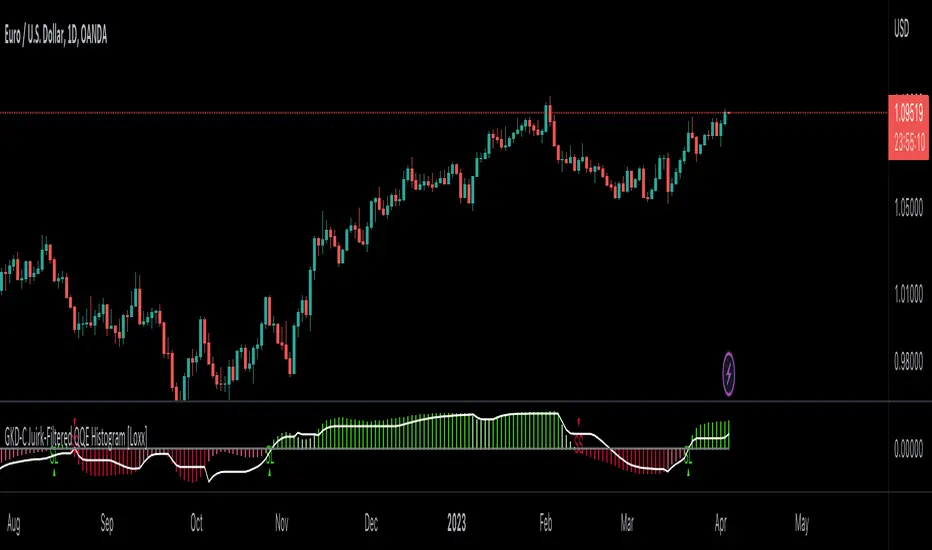
GKD-C RSI of Fast Discrete Cosine Transform [Loxx]Giga Kaleidoscope GKD-C RSI of Fast Discrete Cosine Transform is a Confirmation module included in Loxx's "Giga Kaleidoscope Modularized Trading System".
█ Giga Kaleidoscope Modularized Trading System
What is Loxx's "Giga Kaleidoscope Modularized Trading System"?
The Giga Kaleidoscope Modularized Trading System is a trading system built on the philosophy of the NNFX (No Nonsense Forex) algorithmic trading.
What is the NNFX algorithmic trading strategy?
The NNFX (No-Nonsense Forex) trading system is a comprehensive approach to Forex trading that is designed to simplify the process and remove the confusion and complexity that often surrounds trading. The system was developed by a Forex trader who goes by the pseudonym "VP" and has gained a significant following in the Forex community.
The NNFX trading system is based on a set of rules and guidelines that help traders make objective and informed decisions. These rules cover all aspects of trading, including market analysis, trade entry, stop loss placement, and trade management.
Here are the main components of the NNFX trading system:
1. Trading Philosophy: The NNFX trading system is based on the idea that successful trading requires a comprehensive understanding of the market, objective analysis, and strict risk management. The system aims to remove subjective elements from trading and focuses on objective rules and guidelines.
2. Technical Analysis: The NNFX trading system relies heavily on technical analysis and uses a range of indicators to identify high-probability trading opportunities. The system uses a combination of trend-following and mean-reverting strategies to identify trades.
3. Market Structure: The NNFX trading system emphasizes the importance of understanding the market structure, including price action, support and resistance levels, and market cycles. The system uses a range of tools to identify the market structure, including trend lines, channels, and moving averages.
4. Trade Entry: The NNFX trading system has strict rules for trade entry. The system uses a combination of technical indicators to identify high-probability trades, and traders must meet specific criteria to enter a trade.
5. Stop Loss Placement: The NNFX trading system places a significant emphasis on risk management and requires traders to place a stop loss order on every trade. The system uses a combination of technical analysis and market structure to determine the appropriate stop loss level.
6. Trade Management: The NNFX trading system has specific rules for managing open trades. The system aims to minimize risk and maximize profit by using a combination of trailing stops, take profit levels, and position sizing.
Overall, the NNFX trading system is designed to be a straightforward and easy-to-follow approach to Forex trading that can be applied by traders of all skill levels.
Core components of an NNFX algorithmic trading strategy
The NNFX algorithm is built on the principles of trend, momentum, and volatility. There are six core components in the NNFX trading algorithm:
1. Volatility - price volatility; e.g., Average True Range, True Range Double, Close-to-Close, etc.
2. Baseline - a moving average to identify price trend
3. Confirmation 1 - a technical indicator used to identify trends
4. Confirmation 2 - a technical indicator used to identify trends
5. Continuation - a technical indicator used to identify trends
6. Volatility/Volume - a technical indicator used to identify volatility/volume breakouts/breakdown
7. Exit - a technical indicator used to determine when a trend is exhausted
What is Volatility in the NNFX trading system?
In the NNFX (No Nonsense Forex) trading system, ATR (Average True Range) is typically used to measure the volatility of an asset. It is used as a part of the system to help determine the appropriate stop loss and take profit levels for a trade. ATR is calculated by taking the average of the true range values over a specified period.
True range is calculated as the maximum of the following values:
-Current high minus the current low
-Absolute value of the current high minus the previous close
-Absolute value of the current low minus the previous close
ATR is a dynamic indicator that changes with changes in volatility. As volatility increases, the value of ATR increases, and as volatility decreases, the value of ATR decreases. By using ATR in NNFX system, traders can adjust their stop loss and take profit levels according to the volatility of the asset being traded. This helps to ensure that the trade is given enough room to move, while also minimizing potential losses.
Other types of volatility include True Range Double (TRD), Close-to-Close, and Garman-Klass
What is a Baseline indicator?
The baseline is essentially a moving average, and is used to determine the overall direction of the market.
The baseline in the NNFX system is used to filter out trades that are not in line with the long-term trend of the market. The baseline is plotted on the chart along with other indicators, such as the Moving Average (MA), the Relative Strength Index (RSI), and the Average True Range (ATR).
Trades are only taken when the price is in the same direction as the baseline. For example, if the baseline is sloping upwards, only long trades are taken, and if the baseline is sloping downwards, only short trades are taken. This approach helps to ensure that trades are in line with the overall trend of the market, and reduces the risk of entering trades that are likely to fail.
By using a baseline in the NNFX system, traders can have a clear reference point for determining the overall trend of the market, and can make more informed trading decisions. The baseline helps to filter out noise and false signals, and ensures that trades are taken in the direction of the long-term trend.
What is a Confirmation indicator?
Confirmation indicators are technical indicators that are used to confirm the signals generated by primary indicators. Primary indicators are the core indicators used in the NNFX system, such as the Average True Range (ATR), the Moving Average (MA), and the Relative Strength Index (RSI).
The purpose of the confirmation indicators is to reduce false signals and improve the accuracy of the trading system. They are designed to confirm the signals generated by the primary indicators by providing additional information about the strength and direction of the trend.
Some examples of confirmation indicators that may be used in the NNFX system include the Bollinger Bands, the MACD (Moving Average Convergence Divergence), and the Stochastic Oscillator. These indicators can provide information about the volatility, momentum, and trend strength of the market, and can be used to confirm the signals generated by the primary indicators.
In the NNFX system, confirmation indicators are used in combination with primary indicators and other filters to create a trading system that is robust and reliable. By using multiple indicators to confirm trading signals, the system aims to reduce the risk of false signals and improve the overall profitability of the trades.
What is a Continuation indicator?
In the NNFX (No Nonsense Forex) trading system, a continuation indicator is a technical indicator that is used to confirm a current trend and predict that the trend is likely to continue in the same direction. A continuation indicator is typically used in conjunction with other indicators in the system, such as a baseline indicator, to provide a comprehensive trading strategy.
What is a Volatility/Volume indicator?
Volume indicators, such as the On Balance Volume (OBV), the Chaikin Money Flow (CMF), or the Volume Price Trend (VPT), are used to measure the amount of buying and selling activity in a market. They are based on the trading volume of the market, and can provide information about the strength of the trend. In the NNFX system, volume indicators are used to confirm trading signals generated by the Moving Average and the Relative Strength Index. Volatility indicators include Average Direction Index, Waddah Attar, and Volatility Ratio. In the NNFX trading system, volatility is a proxy for volume and vice versa.
By using volume indicators as confirmation tools, the NNFX trading system aims to reduce the risk of false signals and improve the overall profitability of trades. These indicators can provide additional information about the market that is not captured by the primary indicators, and can help traders to make more informed trading decisions. In addition, volume indicators can be used to identify potential changes in market trends and to confirm the strength of price movements.
What is an Exit indicator?
The exit indicator is used in conjunction with other indicators in the system, such as the Moving Average (MA), the Relative Strength Index (RSI), and the Average True Range (ATR), to provide a comprehensive trading strategy.
The exit indicator in the NNFX system can be any technical indicator that is deemed effective at identifying optimal exit points. Examples of exit indicators that are commonly used include the Parabolic SAR, the Average Directional Index (ADX), and the Chandelier Exit.
The purpose of the exit indicator is to identify when a trend is likely to reverse or when the market conditions have changed, signaling the need to exit a trade. By using an exit indicator, traders can manage their risk and prevent significant losses.
In the NNFX system, the exit indicator is used in conjunction with a stop loss and a take profit order to maximize profits and minimize losses. The stop loss order is used to limit the amount of loss that can be incurred if the trade goes against the trader, while the take profit order is used to lock in profits when the trade is moving in the trader's favor.
Overall, the use of an exit indicator in the NNFX trading system is an important component of a comprehensive trading strategy. It allows traders to manage their risk effectively and improve the profitability of their trades by exiting at the right time.
How does Loxx's GKD (Giga Kaleidoscope Modularized Trading System) implement the NNFX algorithm outlined above?
Loxx's GKD v1.0 system has five types of modules (indicators/strategies). These modules are:
1. GKD-BT - Backtesting module (Volatility, Number 1 in the NNFX algorithm)
2. GKD-B - Baseline module (Baseline and Volatility/Volume, Numbers 1 and 2 in the NNFX algorithm)
3. GKD-C - Confirmation 1/2 and Continuation module (Confirmation 1/2 and Continuation, Numbers 3, 4, and 5 in the NNFX algorithm)
4. GKD-V - Volatility/Volume module (Confirmation 1/2, Number 6 in the NNFX algorithm)
5. GKD-E - Exit module (Exit, Number 7 in the NNFX algorithm)
(additional module types will added in future releases)
Each module interacts with every module by passing data between modules. Data is passed between each module as described below:
GKD-B => GKD-V => GKD-C(1) => GKD-C(2) => GKD-C(Continuation) => GKD-E => GKD-BT
That is, the Baseline indicator passes its data to Volatility/Volume. The Volatility/Volume indicator passes its values to the Confirmation 1 indicator. The Confirmation 1 indicator passes its values to the Confirmation 2 indicator. The Confirmation 2 indicator passes its values to the Continuation indicator. The Continuation indicator passes its values to the Exit indicator, and finally, the Exit indicator passes its values to the Backtest strategy.
This chaining of indicators requires that each module conform to Loxx's GKD protocol, therefore allowing for the testing of every possible combination of technical indicators that make up the six components of the NNFX algorithm.
What does the application of the GKD trading system look like?
Example trading system:
Backtest: Strategy with 1-3 take profits, trailing stop loss, multiple types of PnL volatility, and 2 backtesting styles
Baseline: Hull Moving Average
Volatility/Volume: Hurst Exponent
Confirmation 1: RSI of Fast Discrete Cosine Transform as shown on the chart above
Confirmation 2: Williams Percent Range
Continuation: Fisher Transform
Exit: Rex Oscillator
Each GKD indicator is denoted with a module identifier of either: GKD-BT, GKD-B, GKD-C, GKD-V, or GKD-E. This allows traders to understand to which module each indicator belongs and where each indicator fits into the GKD protocol chain.
Giga Kaleidoscope Modularized Trading System Signals (based on the NNFX algorithm)
Standard Entry
1. GKD-C Confirmation 1 Signal
2. GKD-B Baseline agrees
3. Price is within a range of 0.2x Volatility and 1.0x Volatility of the Goldie Locks Mean
4. GKD-C Confirmation 2 agrees
5. GKD-V Volatility/Volume agrees
Baseline Entry
1. GKD-B Baseline signal
2. GKD-C Confirmation 1 agrees
3. Price is within a range of 0.2x Volatility and 1.0x Volatility of the Goldie Locks Mean
4. GKD-C Confirmation 2 agrees
5. GKD-V Volatility/Volume agrees
6. GKD-C Confirmation 1 signal was less than 7 candles prior
Continuation Entry
1. Standard Entry, Baseline Entry, or Pullback; entry triggered previously
2. GKD-B Baseline hasn't crossed since entry signal trigger
3. GKD-C Confirmation Continuation Indicator signals
4. GKD-C Confirmation 1 agrees
5. GKD-B Baseline agrees
6. GKD-C Confirmation 2 agrees
1-Candle Rule Standard Entry
1. GKD-C Confirmation 1 signal
2. GKD-B Baseline agrees
3. Price is within a range of 0.2x Volatility and 1.0x Volatility of the Goldie Locks Mean
Next Candle:
1. Price retraced (Long: close < close or Short: close > close )
2. GKD-B Baseline agrees
3. GKD-C Confirmation 1 agrees
4. GKD-C Confirmation 2 agrees
5. GKD-V Volatility/Volume agrees
1-Candle Rule Baseline Entry
1. GKD-B Baseline signal
2. GKD-C Confirmation 1 agrees
3. Price is within a range of 0.2x Volatility and 1.0x Volatility of the Goldie Locks Mean
4. GKD-C Confirmation 1 signal was less than 7 candles prior
Next Candle:
1. Price retraced (Long: close < close or Short: close > close )
2. GKD-B Baseline agrees
3. GKD-C Confirmation 1 agrees
4. GKD-C Confirmation 2 agrees
5. GKD-V Volatility/Volume Agrees
PullBack Entry
1. GKD-B Baseline signal
2. GKD-C Confirmation 1 agrees
3. Price is beyond 1.0x Volatility of Baseline
Next Candle:
1. Price is within a range of 0.2x Volatility and 1.0x Volatility of the Goldie Locks Mean
3. GKD-C Confirmation 1 agrees
4. GKD-C Confirmation 2 agrees
5. GKD-V Volatility/Volume Agrees
█ Fast Discrete Cosine Transform
What is the Fast Discrete Cosine Transform?
Algolib is a C++ library for algorithmic trading that provides various algorithms for processing and analyzing financial data. The library includes a Fast Discrete Cosine Transform (FDCT) implementation, which is a fast version of the Discrete Cosine Transform (DCT) algorithm used for signal processing and data compression.
The FDCT implementation in Algolib is based on the FFT (Fast Fourier Transform) algorithm, which is a widely used method for computing the DCT. The implementation is optimized for performance and can handle large datasets efficiently. It uses the standard divide-and-conquer approach to compute the DCT recursively and combines the resulting coefficients to obtain the final DCT of the input signal.
The input to the FDCT algorithm in Algolib is a one-dimensional array of real numbers, which represents a time series or a financial signal. The algorithm then computes the DCT of the input sequence and returns a one-dimensional array of DCT coefficients, which represent the frequency components of the signal.
The implementation of the FDCT algorithm in Algolib uses C++ templates to provide a generic implementation that can work with different data types. It also includes various optimizations, such as loop unrolling, to improve the performance of the algorithm.
The steps involved in the FDCT algorithm in Algolib are:
-Divide the input sequence into even and odd parts.
-Compute the DCT of the even and odd parts recursively.
-Combine the DCT coefficients of the even and odd parts to obtain the final DCT coefficients.
-The implementation of the FDCT algorithm in Algolib uses the FFTW (Fastest Fourier Transform in the West) library to perform the FFT computations, which is a highly optimized library for computing Fourier transforms.
In summary, the Fast Discrete Cosine Transform implementation in Algolib is a fast and efficient implementation of the DCT algorithm, which is used for processing financial signals and time series data. The implementation is optimized for performance and uses the FFT algorithm for fast computation. The implementation is generic and can work with different data types, and includes optimizations such as loop unrolling to improve the performance of the algorithm.
What is the Fast Discrete Cosine Transform in terms of Forex trading?
The Fast Discrete Cosine Transform (FDCT) is an algorithm used for signal processing and data compression that can also be applied in trading forex. The FDCT is used to transform financial data into a set of coefficients that represent the data in terms of cosine functions of different frequencies. These coefficients can be used to analyze the frequency components of financial signals and to develop trading strategies based on these components.
In trading forex, the FDCT can be applied to various financial signals, such as price data, volume data, and technical indicators. By applying the FDCT to these signals, traders can identify the dominant frequency components of the signals and use this information to develop trading strategies.
For example, traders can use the FDCT to identify cycles in the market and use this information to develop trend-following strategies. The FDCT can also be used to identify short-term fluctuations in the market and develop mean-reversion strategies based on these fluctuations.
The FDCT can also be used in combination with other technical analysis tools, such as moving averages, to improve the accuracy of trading signals. For example, traders can apply the FDCT to the moving average of a financial signal to identify the dominant frequency components of the moving average and use this information to develop trading signals.
The FDCT can also be used in conjunction with machine learning algorithms to develop predictive models for financial markets. By applying the FDCT to financial data and using the resulting coefficients as inputs to a machine learning algorithm, traders can develop models that predict future price movements and identify profitable trading opportunities.
In summary, the FDCT can be applied in trading forex to analyze the frequency components of financial signals and develop trading strategies based on these components. The FDCT can be used in conjunction with other technical analysis tools and machine learning algorithms to improve the accuracy of trading signals and develop predictive models for financial markets.
█ Relative Strength Index (RSI)
This indicator contains 7 different types of RSI .
RSX
Regular
Slow
Rapid
Harris
Cuttler
Ehlers Smoothed
What is RSI?
RSI stands for Relative Strength Index . It is a technical indicator used to measure the strength or weakness of a financial instrument's price action.
The RSI is calculated based on the price movement of an asset over a specified period of time, typically 14 days, and is expressed on a scale of 0 to 100. The RSI is considered overbought when it is above 70 and oversold when it is below 30.
Traders and investors use the RSI to identify potential buy and sell signals. When the RSI indicates that an asset is oversold, it may be considered a buying opportunity, while an overbought RSI may signal that it is time to sell or take profits.
It's important to note that the RSI should not be used in isolation and should be used in conjunction with other technical and fundamental analysis tools to make informed trading decisions.
What is RSX?
Jurik RSX is a technical analysis indicator that is a variation of the Relative Strength Index Smoothed ( RSX ) indicator. It was developed by Mark Jurik and is designed to help traders identify trends and momentum in the market.
The Jurik RSX uses a combination of the RSX indicator and an adaptive moving average (AMA) to smooth out the price data and reduce the number of false signals. The adaptive moving average is designed to adjust the smoothing period based on the current market conditions, which makes the indicator more responsive to changes in price.
The Jurik RSX can be used to identify potential trend reversals and momentum shifts in the market. It oscillates between 0 and 100, with values above 50 indicating a bullish trend and values below 50 indicating a bearish trend . Traders can use these levels to make trading decisions, such as buying when the indicator crosses above 50 and selling when it crosses below 50.
The Jurik RSX is a more advanced version of the RSX indicator, and while it can be useful in identifying potential trade opportunities, it should not be used in isolation. It is best used in conjunction with other technical and fundamental analysis tools to make informed trading decisions.
What is Slow RSI?
Slow RSI is a variation of the traditional Relative Strength Index ( RSI ) indicator. It is a more smoothed version of the RSI and is designed to filter out some of the noise and short-term price fluctuations that can occur with the standard RSI .
The Slow RSI uses a longer period of time than the traditional RSI , typically 21 periods instead of 14. This longer period helps to smooth out the price data and makes the indicator less reactive to short-term price fluctuations.
Like the traditional RSI , the Slow RSI is used to identify potential overbought and oversold conditions in the market. It oscillates between 0 and 100, with values above 70 indicating overbought conditions and values below 30 indicating oversold conditions. Traders often use these levels as potential buy and sell signals.
The Slow RSI is a more conservative version of the RSI and can be useful in identifying longer-term trends in the market. However, it can also be slower to respond to changes in price, which may result in missed trading opportunities. Traders may choose to use a combination of both the Slow RSI and the traditional RSI to make informed trading decisions.
What is Rapid RSI?
Same as regular RSI but with a faster calculation method
What is Harris RSI?
Harris RSI is a technical analysis indicator that is a variation of the Relative Strength Index ( RSI ). It was developed by Larry Harris and is designed to help traders identify potential trend changes and momentum shifts in the market.
The Harris RSI uses a different calculation formula compared to the traditional RSI . It takes into account both the opening and closing prices of a financial instrument, as well as the high and low prices. The Harris RSI is also normalized to a range of 0 to 100, with values above 50 indicating a bullish trend and values below 50 indicating a bearish trend .
Like the traditional RSI , the Harris RSI is used to identify potential overbought and oversold conditions in the market. It oscillates between 0 and 100, with values above 70 indicating overbought conditions and values below 30 indicating oversold conditions. Traders often use these levels as potential buy and sell signals.
The Harris RSI is a more advanced version of the RSI and can be useful in identifying longer-term trends in the market. However, it can also generate more false signals than the standard RSI . Traders may choose to use a combination of both the Harris RSI and the traditional RSI to make informed trading decisions.
What is Cuttler RSI?
Cuttler RSI is a technical analysis indicator that is a variation of the Relative Strength Index ( RSI ). It was developed by Curt Cuttler and is designed to help traders identify potential trend changes and momentum shifts in the market.
The Cuttler RSI uses a different calculation formula compared to the traditional RSI . It takes into account the difference between the closing price of a financial instrument and the average of the high and low prices over a specified period of time. This difference is then normalized to a range of 0 to 100, with values above 50 indicating a bullish trend and values below 50 indicating a bearish trend .
Like the traditional RSI , the Cuttler RSI is used to identify potential overbought and oversold conditions in the market. It oscillates between 0 and 100, with values above 70 indicating overbought conditions and values below 30 indicating oversold conditions. Traders often use these levels as potential buy and sell signals.
The Cuttler RSI is a more advanced version of the RSI and can be useful in identifying longer-term trends in the market. However, it can also generate more false signals than the standard RSI . Traders may choose to use a combination of both the Cuttler RSI and the traditional RSI to make informed trading decisions.
What is Ehlers Smoothed RSI?
Ehlers smoothed RSI is a technical analysis indicator that is a variation of the Relative Strength Index ( RSI ). It was developed by John Ehlers and is designed to help traders identify potential trend changes and momentum shifts in the market.
The Ehlers smoothed RSI uses a different calculation formula compared to the traditional RSI . It uses a smoothing algorithm that is designed to reduce the noise and random fluctuations that can occur with the standard RSI . The smoothing algorithm is based on a concept called "digital signal processing" and is intended to improve the accuracy of the indicator.
Like the traditional RSI , the Ehlers smoothed RSI is used to identify potential overbought and oversold conditions in the market. It oscillates between 0 and 100, with values above 70 indicating overbought conditions and values below 30 indicating oversold conditions. Traders often use these levels as potential buy and sell signals.
The Ehlers smoothed RSI can be useful in identifying longer-term trends and momentum shifts in the market. However, it can also generate more false signals than the standard RSI . Traders may choose to use a combination of both the Ehlers smoothed RSI and the traditional RSI to make informed trading decisions.
█ GKD-C RSI of Fast Discrete Cosine Transform
What is the RSI of Fast Discrete Cosine Transform in terms of Forex trading?
The Relative Strength Index (RSI) is a popular technical indicator used in trading forex to measure the strength of a trend and identify potential trend reversals. While the Fast Discrete Cosine Transform (FDCT) is not directly related to the RSI, it can be used to analyze the frequency components of the price data used to calculate the RSI and improve its accuracy.
The RSI is calculated by comparing the average gains and losses of a financial instrument over a given period of time. The RSI value ranges from 0 to 100, with values above 70 indicating an overbought market and values below 30 indicating an oversold market.
One limitation of the RSI is that it only considers the average gains and losses over a fixed period of time, which may not capture the complex patterns and dynamics of financial markets. This is where the FDCT can be useful.
By applying the FDCT to the price data used to calculate the RSI, traders can identify the dominant frequency components of the price data and use this information to adjust the RSI calculation. For example, traders can weight the gains and losses based on the frequency components identified by the FDCT, giving more weight to the dominant frequencies and less weight to the lower frequencies.
This approach can improve the accuracy of the RSI calculation and provide traders with more reliable signals for identifying trends and potential trend reversals. Traders can also use the frequency components identified by the FDCT to develop more advanced trading strategies, such as identifying cycles in the market and using this information to develop trend-following strategies.
In summary, while the FDCT is not directly related to the RSI, it can be used to analyze the frequency components of the price data used to calculate the RSI and improve its accuracy. Traders can use the FDCT to identify dominant frequency components and adjust the RSI calculation accordingly, providing more reliable signals for identifying trends and potential trend reversals.
This indicator has period lengths that are powers of powers of 2. There is also a features to increase the resolution of the FDCT.
Requirements
Inputs
Confirmation 1 and Solo Confirmation: GKD-V Volatility / Volume indicator
Confirmation 2: GKD-C Confirmation indicator
Outputs
Confirmation 2 and Solo Confirmation Complex: GKD-E Exit indicator
Confirmation 1: GKD-C Confirmation indicator
Continuation: GKD-E Exit indicator
Solo Confirmation Simple: GKD-BT Backtest strategy
Additional features will be added in future releases.