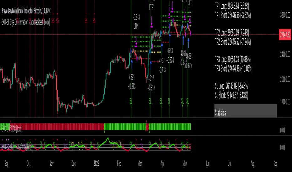
GKD-BT Giga Confirmation Stack Backtest [Loxx]Giga Kaleidoscope GKD-BT Giga Confirmation Stack Backtest is a Backtesting module included in Loxx's "Giga Kaleidoscope Modularized Trading System".
█ GKD-BT Giga Confirmation Stack Backtest
The Giga Confirmation Stack Backtest module allows users to perform backtesting on Long and Short signals from the confluence between GKD-C Confirmation 1 and GKD-C Confirmation 2 indicators. This module encompasses two types of backtests: Trading and Full. The Trading backtest permits users to evaluate individual trades, whether Long or Short, one at a time. Conversely, the Full backtest allows users to analyze either Longs or Shorts separately by toggling between them in the settings, enabling the examination of results for each signal type. The Trading backtest emulates actual trading conditions, while the Full backtest assesses all signals, regardless of being Long or Short.
Additionally, this backtest module provides the option to test using indicators with 1 to 3 take profits and 1 stop loss. The Trading backtest allows for the use of 1 to 3 take profits, while the Full backtest is limited to 1 take profit. The Trading backtest also offers the capability to apply a trailing take profit.
In terms of the percentage of trade removed at each take profit, this backtest module has the following hardcoded values:
Take profit 1: 50% of the trade is removed.
Take profit 2: 25% of the trade is removed.
Take profit 3: 25% of the trade is removed.
Stop loss: 100% of the trade is removed.
After each take profit is achieved, the stop loss level is adjusted. When take profit 1 is reached, the stop loss is moved to the entry point. Similarly, when take profit 2 is reached, the stop loss is shifted to take profit 1. The trailing take profit feature comes into play after take profit 2 or take profit 3, depending on the number of take profits selected in the settings. The trailing take profit is always activated on the final take profit when 2 or more take profits are chosen.
The backtest module also offers the capability to restrict by a specific date range, allowing for simulated forward testing based on past data. Additionally, users have the option to display or hide a trading panel that provides relevant information about the backtest, statistics, and the current trade. It is also possible to activate alerts and toggle sections of the trading panel on or off. On the chart, historical take profit and stop loss levels are represented by horizontal lines overlaid for reference.
To utilize this strategy, follow these steps:
1. Adjust the "Confirmation Type" in the GKD-C Confirmation 1 Indicator to "GKD New."
2. GKD-C Confirmation 1 Import: Import the value "Input into NEW GKD-BT Backtest" from the GKD-C Confirmation 1 module into the GKD-BT Giga Confirmation Stack Backtest module setting named "Import GKD-C Confirmation 1."
3. Adjust the "Confirmation Type" in the GKD-C Confirmation 2 Indicator to "GKD New."
4. GKD-C Confirmation 2 Import: Import the value "Input into NEW GKD-BT Backtest" from the GKD-C Confirmation 2 module into the GKD-BT Giga Confirmation Stack Backtest module setting named "Import GKD-C Confirmation 2."
█ Giga Confirmation Stack Backtest Entries
Entries are generated from the confluence of a GKD-C Confirmation 1 and GKD-C Confirmation 2 indicators. The Confirmation 1 gives the signal and the Confirmation 2 indicator filters or "approves" the the Confirmation 1 signal. If Confirmation 1 gives a long signal and Confirmation 2 shows a downtrend, then the long signal is rejected. If Confirmation 1 gives a long signal and Confirmation 2 shows an uptrend, then the long signal is approved and sent to the backtest execution engine.
█ Volatility Types Included
The GKD system utilizes volatility-based take profits and stop losses. Each take profit and stop loss is calculated as a multiple of volatility. Users can also adjust the multiplier values in the settings.
This module includes 17 types of volatility:
Close-to-Close
Parkinson
Garman-Klass
Rogers-Satchell
Yang-Zhang
Garman-Klass-Yang-Zhang
Exponential Weighted Moving Average
Standard Deviation of Log Returns
Pseudo GARCH(2,2)
Average True Range
True Range Double
Standard Deviation
Adaptive Deviation
Median Absolute Deviation
Efficiency-Ratio Adaptive ATR
Mean Absolute Deviation
Static Percent
Close-to-Close
Close-to-Close volatility is a classic and widely used volatility measure, sometimes referred to as historical volatility.
Volatility is an indicator of the speed of a stock price change. A stock with high volatility is one where the price changes rapidly and with a larger amplitude. The more volatile a stock is, the riskier it is.
Close-to-close historical volatility is calculated using only a stock's closing prices. It is the simplest volatility estimator. However, in many cases, it is not precise enough. Stock prices could jump significantly during a trading session and return to the opening value at the end. That means that a considerable amount of price information is not taken into account by close-to-close volatility.
Despite its drawbacks, Close-to-Close volatility is still useful in cases where the instrument doesn't have intraday prices. For example, mutual funds calculate their net asset values daily or weekly, and thus their prices are not suitable for more sophisticated volatility estimators.
Parkinson
Parkinson volatility is a volatility measure that uses the stock’s high and low price of the day.
The main difference between regular volatility and Parkinson volatility is that the latter uses high and low prices for a day, rather than only the closing price. This is useful as close-to-close prices could show little difference while large price movements could have occurred during the day. Thus, Parkinson's volatility is considered more precise and requires less data for calculation than close-to-close volatility.
One drawback of this estimator is that it doesn't take into account price movements after the market closes. Hence, it systematically undervalues volatility. This drawback is addressed in the Garman-Klass volatility estimator.
Garman-Klass
Garman-Klass is a volatility estimator that incorporates open, low, high, and close prices of a security.
Garman-Klass volatility extends Parkinson's volatility by taking into account the opening and closing prices. As markets are most active during the opening and closing of a trading session, it makes volatility estimation more accurate.
Garman and Klass also assumed that the process of price change follows a continuous diffusion process (Geometric Brownian motion). However, this assumption has several drawbacks. The method is not robust for opening jumps in price and trend movements.
Despite its drawbacks, the Garman-Klass estimator is still more effective than the basic formula since it takes into account not only the price at the beginning and end of the time interval but also intraday price extremes.
Researchers Rogers and Satchell have proposed a more efficient method for assessing historical volatility that takes into account price trends. See Rogers-Satchell Volatility for more detail.
Rogers-Satchell
Rogers-Satchell is an estimator for measuring the volatility of securities with an average return not equal to zero.
Unlike Parkinson and Garman-Klass estimators, Rogers-Satchell incorporates a drift term (mean return not equal to zero). As a result, it provides better volatility estimation when the underlying is trending.
The main disadvantage of this method is that it does not take into account price movements between trading sessions. This leads to an underestimation of volatility since price jumps periodically occur in the market precisely at the moments between sessions.
A more comprehensive estimator that also considers the gaps between sessions was developed based on the Rogers-Satchel formula in the 2000s by Yang-Zhang. See Yang Zhang Volatility for more detail.
Yang-Zhang
Yang Zhang is a historical volatility estimator that handles both opening jumps and the drift and has a minimum estimation error.
Yang-Zhang volatility can be thought of as a combination of the overnight (close-to-open volatility) and a weighted average of the Rogers-Satchell volatility and the day’s open-to-close volatility. It is considered to be 14 times more efficient than the close-to-close estimator.
Garman-Klass-Yang-Zhang
Garman-Klass-Yang-Zhang (GKYZ) volatility estimator incorporates the returns of open, high, low, and closing prices in its calculation.
GKYZ volatility estimator takes into account overnight jumps but not the trend, i.e., it assumes that the underlying asset follows a Geometric Brownian Motion (GBM) process with zero drift. Therefore, the GKYZ volatility estimator tends to overestimate the volatility when the drift is different from zero. However, for a GBM process, this estimator is eight times more efficient than the close-to-close volatility estimator.
Exponential Weighted Moving Average
The Exponentially Weighted Moving Average (EWMA) is a quantitative or statistical measure used to model or describe a time series. The EWMA is widely used in finance, with the main applications being technical analysis and volatility modeling.
The moving average is designed such that older observations are given lower weights. The weights decrease exponentially as the data point gets older – hence the name exponentially weighted.
The only decision a user of the EWMA must make is the parameter lambda. The parameter decides how important the current observation is in the calculation of the EWMA. The higher the value of lambda, the more closely the EWMA tracks the original time series.
Standard Deviation of Log Returns
This is the simplest calculation of volatility. It's the standard deviation of ln(close/close(1)).
Pseudo GARCH(2,2)
This is calculated using a short- and long-run mean of variance multiplied by ?.
?avg(var;M) + (1 ? ?) avg(var;N) = 2?var/(M+1-(M-1)L) + 2(1-?)var/(M+1-(M-1)L)
Solving for ? can be done by minimizing the mean squared error of estimation; that is, regressing L^-1var - avg(var; N) against avg(var; M) - avg(var; N) and using the resulting beta estimate as ?.
Average True Range
The average true range (ATR) is a technical analysis indicator, introduced by market technician J. Welles Wilder Jr. in his book New Concepts in Technical Trading Systems, that measures market volatility by decomposing the entire range of an asset price for that period.
The true range indicator is taken as the greatest of the following: current high less the current low; the absolute value of the current high less the previous close; and the absolute value of the current low less the previous close. The ATR is then a moving average, generally using 14 days, of the true ranges.
True Range Double
A special case of ATR that attempts to correct for volatility skew.
Standard Deviation
Standard deviation is a statistic that measures the dispersion of a dataset relative to its mean and is calculated as the square root of the variance. The standard deviation is calculated as the square root of variance by determining each data point's deviation relative to the mean. If the data points are further from the mean, there is a higher deviation within the data set; thus, the more spread out the data, the higher the standard deviation.
Adaptive Deviation
By definition, the Standard Deviation (STD, also represented by the Greek letter sigma ? or the Latin letter s) is a measure that is used to quantify the amount of variation or dispersion of a set of data values. In technical analysis, we usually use it to measure the level of current volatility.
Standard Deviation is based on Simple Moving Average calculation for mean value. This version of standard deviation uses the properties of EMA to calculate what can be called a new type of deviation, and since it is based on EMA, we can call it EMA deviation. Additionally, Perry Kaufman's efficiency ratio is used to make it adaptive (since all EMA type calculations are nearly perfect for adapting).
The difference when compared to the standard is significant--not just because of EMA usage, but the efficiency ratio makes it a "bit more logical" in very volatile market conditions.
Median Absolute Deviation
The median absolute deviation is a measure of statistical dispersion. Moreover, the MAD is a robust statistic, being more resilient to outliers in a data set than the standard deviation. In the standard deviation, the distances from the mean are squared, so large deviations are weighted more heavily, and thus outliers can heavily influence it. In the MAD, the deviations of a small number of outliers are irrelevant.
Because the MAD is a more robust estimator of scale than the sample variance or standard deviation, it works better with distributions without a mean or variance, such as the Cauchy distribution.
Efficiency-Ratio Adaptive ATR
Average True Range (ATR) is a widely used indicator for many occasions in technical analysis. It is calculated as the RMA of the true range. This version adds a "twist": it uses Perry Kaufman's Efficiency Ratio to calculate adaptive true range.
Mean Absolute Deviation
The mean absolute deviation (MAD) is a measure of variability that indicates the average distance between observations and their mean. MAD uses the original units of the data, which simplifies interpretation. Larger values signify that the data points spread out further from the average. Conversely, lower values correspond to data points bunching closer to it. The mean absolute deviation is also known as the mean deviation and average absolute deviation.
This definition of the mean absolute deviation sounds similar to the standard deviation (SD). While both measure variability, they have different calculations. In recent years, some proponents of MAD have suggested that it replace the SD as the primary measure because it is a simpler concept that better fits real life.
Static Percent
Static Percent allows the user to insert their own constant percent that will then be used to create take profits and stoploss
█ Giga Kaleidoscope Modularized Trading System
Core components of an NNFX algorithmic trading strategy
The NNFX algorithm is built on the principles of trend, momentum, and volatility. There are six core components in the NNFX trading algorithm:
1. Volatility - price volatility; e.g., Average True Range, True Range Double, Close-to-Close, etc.
2. Baseline - a moving average to identify price trend
3. Confirmation 1 - a technical indicator used to identify trends
4. Confirmation 2 - a technical indicator used to identify trends
5. Continuation - a technical indicator used to identify trends
6. Volatility/Volume - a technical indicator used to identify volatility/volume breakouts/breakdown
7. Exit - a technical indicator used to determine when a trend is exhausted
What is Volatility in the NNFX trading system?
In the NNFX (No Nonsense Forex) trading system, ATR (Average True Range) is typically used to measure the volatility of an asset. It is used as a part of the system to help determine the appropriate stop loss and take profit levels for a trade. ATR is calculated by taking the average of the true range values over a specified period.
True range is calculated as the maximum of the following values:
-Current high minus the current low
-Absolute value of the current high minus the previous close
-Absolute value of the current low minus the previous close
ATR is a dynamic indicator that changes with changes in volatility. As volatility increases, the value of ATR increases, and as volatility decreases, the value of ATR decreases. By using ATR in NNFX system, traders can adjust their stop loss and take profit levels according to the volatility of the asset being traded. This helps to ensure that the trade is given enough room to move, while also minimizing potential losses.
Other types of volatility include True Range Double (TRD), Close-to-Close, and Garman-Klass
What is a Baseline indicator?
The baseline is essentially a moving average, and is used to determine the overall direction of the market.
The baseline in the NNFX system is used to filter out trades that are not in line with the long-term trend of the market. The baseline is plotted on the chart along with other indicators, such as the Moving Average (MA), the Relative Strength Index (RSI), and the Average True Range (ATR).
Trades are only taken when the price is in the same direction as the baseline. For example, if the baseline is sloping upwards, only long trades are taken, and if the baseline is sloping downwards, only short trades are taken. This approach helps to ensure that trades are in line with the overall trend of the market, and reduces the risk of entering trades that are likely to fail.
By using a baseline in the NNFX system, traders can have a clear reference point for determining the overall trend of the market, and can make more informed trading decisions. The baseline helps to filter out noise and false signals, and ensures that trades are taken in the direction of the long-term trend.
What is a Confirmation indicator?
Confirmation indicators are technical indicators that are used to confirm the signals generated by primary indicators. Primary indicators are the core indicators used in the NNFX system, such as the Average True Range (ATR), the Moving Average (MA), and the Relative Strength Index (RSI).
The purpose of the confirmation indicators is to reduce false signals and improve the accuracy of the trading system. They are designed to confirm the signals generated by the primary indicators by providing additional information about the strength and direction of the trend.
Some examples of confirmation indicators that may be used in the NNFX system include the Bollinger Bands, the MACD (Moving Average Convergence Divergence), and the MACD Oscillator. These indicators can provide information about the volatility, momentum, and trend strength of the market, and can be used to confirm the signals generated by the primary indicators.
In the NNFX system, confirmation indicators are used in combination with primary indicators and other filters to create a trading system that is robust and reliable. By using multiple indicators to confirm trading signals, the system aims to reduce the risk of false signals and improve the overall profitability of the trades.
What is a Continuation indicator?
In the NNFX (No Nonsense Forex) trading system, a continuation indicator is a technical indicator that is used to confirm a current trend and predict that the trend is likely to continue in the same direction. A continuation indicator is typically used in conjunction with other indicators in the system, such as a baseline indicator, to provide a comprehensive trading strategy.
What is a Volatility/Volume indicator?
Volume indicators, such as the On Balance Volume (OBV), the Chaikin Money Flow (CMF), or the Volume Price Trend (VPT), are used to measure the amount of buying and selling activity in a market. They are based on the trading volume of the market, and can provide information about the strength of the trend. In the NNFX system, volume indicators are used to confirm trading signals generated by the Moving Average and the Relative Strength Index. Volatility indicators include Average Direction Index, Waddah Attar, and Volatility Ratio. In the NNFX trading system, volatility is a proxy for volume and vice versa.
By using volume indicators as confirmation tools, the NNFX trading system aims to reduce the risk of false signals and improve the overall profitability of trades. These indicators can provide additional information about the market that is not captured by the primary indicators, and can help traders to make more informed trading decisions. In addition, volume indicators can be used to identify potential changes in market trends and to confirm the strength of price movements.
What is an Exit indicator?
The exit indicator is used in conjunction with other indicators in the system, such as the Moving Average (MA), the Relative Strength Index (RSI), and the Average True Range (ATR), to provide a comprehensive trading strategy.
The exit indicator in the NNFX system can be any technical indicator that is deemed effective at identifying optimal exit points. Examples of exit indicators that are commonly used include the Parabolic SAR, the Average Directional Index (ADX), and the Chandelier Exit.
The purpose of the exit indicator is to identify when a trend is likely to reverse or when the market conditions have changed, signaling the need to exit a trade. By using an exit indicator, traders can manage their risk and prevent significant losses.
In the NNFX system, the exit indicator is used in conjunction with a stop loss and a take profit order to maximize profits and minimize losses. The stop loss order is used to limit the amount of loss that can be incurred if the trade goes against the trader, while the take profit order is used to lock in profits when the trade is moving in the trader's favor.
Overall, the use of an exit indicator in the NNFX trading system is an important component of a comprehensive trading strategy. It allows traders to manage their risk effectively and improve the profitability of their trades by exiting at the right time.
How does Loxx's GKD (Giga Kaleidoscope Modularized Trading System) implement the NNFX algorithm outlined above?
Loxx's GKD v2.0 system has five types of modules (indicators/strategies). These modules are:
1. GKD-BT - Backtesting module (Volatility, Number 1 in the NNFX algorithm)
2. GKD-B - Baseline module (Baseline and Volatility/Volume, Numbers 1 and 2 in the NNFX algorithm)
3. GKD-C - Confirmation 1/2 and Continuation module (Confirmation 1/2 and Continuation, Numbers 3, 4, and 5 in the NNFX algorithm)
4. GKD-V - Volatility/Volume module (Confirmation 1/2, Number 6 in the NNFX algorithm)
5. GKD-E - Exit module (Exit, Number 7 in the NNFX algorithm)
(additional module types will added in future releases)
Each module interacts with every module by passing data to A backtest module wherein the various components of the GKD system are combined to create a trading signal.
That is, the Baseline indicator passes its data to Volatility/Volume. The Volatility/Volume indicator passes its values to the Confirmation 1 indicator. The Confirmation 1 indicator passes its values to the Confirmation 2 indicator. The Confirmation 2 indicator passes its values to the Continuation indicator. The Continuation indicator passes its values to the Exit indicator, and finally, the Exit indicator passes its values to the Backtest strategy.
This chaining of indicators requires that each module conform to Loxx's GKD protocol, therefore allowing for the testing of every possible combination of technical indicators that make up the six components of the NNFX algorithm.
What does the application of the GKD trading system look like?
Example trading system:
Backtest: Confiramtion Stack Backtest
Baseline: Hull Moving Average
Volatility/Volume: Hurst Exponent
Confirmation 1: Fisher Transform as shown on the chart above
Confirmation 2: uf2018 as shown on the chart above
Continuation: Vortex
Exit: Rex Oscillator
Each GKD indicator is denoted with a module identifier of either: GKD-BT, GKD-B, GKD-C, GKD-V, or GKD-E. This allows traders to understand to which module each indicator belongs and where each indicator fits into the GKD system.
Search in scripts for "range"
GKD-BT Giga Stacks Backtest [Loxx]Giga Kaleidoscope GKD-BT Giga Stacks Backtest is a Backtesting module included in Loxx's "Giga Kaleidoscope Modularized Trading System".
█ GKD-BT Giga Stacks Backtest
The Giga Stacks Backtest module allows users to perform backtesting on Long and Short signals from the confluence of GKD-B Baseline, GKD-C Confirmation, and GKD-V Volatility/Volume indicators. This module encompasses two types of backtests: Trading and Full. The Trading backtest permits users to evaluate individual trades, whether Long or Short, one at a time. Conversely, the Full backtest allows users to analyze either Longs or Shorts separately by toggling between them in the settings, enabling the examination of results for each signal type. The Trading backtest emulates actual trading conditions, while the Full backtest assesses all signals, regardless of being Long or Short.
Additionally, this backtest module provides the option to test using indicators with 1 to 3 take profits and 1 stop loss. The Trading backtest allows for the use of 1 to 3 take profits, while the Full backtest is limited to 1 take profit. The Trading backtest also offers the capability to apply a trailing take profit.
In terms of the percentage of trade removed at each take profit, this backtest module has the following hardcoded values:
Take profit 1: 50% of the trade is removed.
Take profit 2: 25% of the trade is removed.
Take profit 3: 25% of the trade is removed.
Stop loss: 100% of the trade is removed.
After each take profit is achieved, the stop loss level is adjusted. When take profit 1 is reached, the stop loss is moved to the entry point. Similarly, when take profit 2 is reached, the stop loss is shifted to take profit 1. The trailing take profit feature comes into play after take profit 2 or take profit 3, depending on the number of take profits selected in the settings. The trailing take profit is always activated on the final take profit when 2 or more take profits are chosen.
The backtest module also offers the capability to restrict by a specific date range, allowing for simulated forward testing based on past data. Additionally, users have the option to display or hide a trading panel that provides relevant information about the backtest, statistics, and the current trade. It is also possible to activate alerts and toggle sections of the trading panel on or off. On the chart, historical take profit and stop loss levels are represented by horizontal lines overlaid for reference.
To utilize this strategy, follow these steps (where "Stack XX" denotes the number of the Stack):
GKD-B Baseline Import: Import the value "Input into NEW GKD-BT Backtest" from the GKD-B Baseline module into the GKD-BT Giga Stacks Backtest module setting named "Stack XX: Import GKD-C, GKD-B, or GKD-V."
GKD-V Volatility/Volume Import: Import the value "Input into NEW GKD-BT Backtest" from the GKD-V Volatility/Volume module into the GKD-BT Giga Stacks Backtest module setting named "Stack XX: Import GKD-C, GKD-B, or GKD-V."
GKD-C Confirmation Import: 1) Adjust the "Confirmation Type" in the GKD-C Confirmation Indicator to "GKD New."; 2) Import the value "Input into NEW GKD-BT Backtest" from the GKD-C Confirmation module into the GKD-BT Giga Stacks Backtest module setting named "Stack XX: Import GKD-C, GKD-B, or GKD."
█ Giga Stacks Backtest Entries
Entries are generated form the confluence of up to six GKD-B Baseline, GKD-C Confirmation, and GKD-V Volatility/Volume indicators. Signals are generated when all Stacks reach uptrend or downtrend together.
Here's how this works. Assume we have the following Stacks and their respective trend on the current candle:
Stack 1 indicator is in uptreend
Stack 2 indicator is in downtrend
Stack 3 indicator is in uptreend
Stack 4 indicator is in uptreend
All stacks are in uptrend except for Stack 2. If Stack 2 reaches uptrend while Stacks 1, 3, and 4 stay in uptrend, then a long signal is generated. The last Stack to align with all other Stacks will generate a long or short signal.
█ Volatility Types Included
The GKD system utilizes volatility-based take profits and stop losses. Each take profit and stop loss is calculated as a multiple of volatility. Users can also adjust the multiplier values in the settings.
This module includes 17 types of volatility:
Close-to-Close
Parkinson
Garman-Klass
Rogers-Satchell
Yang-Zhang
Garman-Klass-Yang-Zhang
Exponential Weighted Moving Average
Standard Deviation of Log Returns
Pseudo GARCH(2,2)
Average True Range
True Range Double
Standard Deviation
Adaptive Deviation
Median Absolute Deviation
Efficiency-Ratio Adaptive ATR
Mean Absolute Deviation
Static Percent
Close-to-Close
Close-to-Close volatility is a classic and widely used volatility measure, sometimes referred to as historical volatility.
Volatility is an indicator of the speed of a stock price change. A stock with high volatility is one where the price changes rapidly and with a larger amplitude. The more volatile a stock is, the riskier it is.
Close-to-close historical volatility is calculated using only a stock's closing prices. It is the simplest volatility estimator. However, in many cases, it is not precise enough. Stock prices could jump significantly during a trading session and return to the opening value at the end. That means that a considerable amount of price information is not taken into account by close-to-close volatility.
Despite its drawbacks, Close-to-Close volatility is still useful in cases where the instrument doesn't have intraday prices. For example, mutual funds calculate their net asset values daily or weekly, and thus their prices are not suitable for more sophisticated volatility estimators.
Parkinson
Parkinson volatility is a volatility measure that uses the stock’s high and low price of the day.
The main difference between regular volatility and Parkinson volatility is that the latter uses high and low prices for a day, rather than only the closing price. This is useful as close-to-close prices could show little difference while large price movements could have occurred during the day. Thus, Parkinson's volatility is considered more precise and requires less data for calculation than close-to-close volatility.
One drawback of this estimator is that it doesn't take into account price movements after the market closes. Hence, it systematically undervalues volatility. This drawback is addressed in the Garman-Klass volatility estimator.
Garman-Klass
Garman-Klass is a volatility estimator that incorporates open, low, high, and close prices of a security.
Garman-Klass volatility extends Parkinson's volatility by taking into account the opening and closing prices. As markets are most active during the opening and closing of a trading session, it makes volatility estimation more accurate.
Garman and Klass also assumed that the process of price change follows a continuous diffusion process (Geometric Brownian motion). However, this assumption has several drawbacks. The method is not robust for opening jumps in price and trend movements.
Despite its drawbacks, the Garman-Klass estimator is still more effective than the basic formula since it takes into account not only the price at the beginning and end of the time interval but also intraday price extremes.
Researchers Rogers and Satchell have proposed a more efficient method for assessing historical volatility that takes into account price trends. See Rogers-Satchell Volatility for more detail.
Rogers-Satchell
Rogers-Satchell is an estimator for measuring the volatility of securities with an average return not equal to zero.
Unlike Parkinson and Garman-Klass estimators, Rogers-Satchell incorporates a drift term (mean return not equal to zero). As a result, it provides better volatility estimation when the underlying is trending.
The main disadvantage of this method is that it does not take into account price movements between trading sessions. This leads to an underestimation of volatility since price jumps periodically occur in the market precisely at the moments between sessions.
A more comprehensive estimator that also considers the gaps between sessions was developed based on the Rogers-Satchel formula in the 2000s by Yang-Zhang. See Yang Zhang Volatility for more detail.
Yang-Zhang
Yang Zhang is a historical volatility estimator that handles both opening jumps and the drift and has a minimum estimation error.
Yang-Zhang volatility can be thought of as a combination of the overnight (close-to-open volatility) and a weighted average of the Rogers-Satchell volatility and the day’s open-to-close volatility. It is considered to be 14 times more efficient than the close-to-close estimator.
Garman-Klass-Yang-Zhang
Garman-Klass-Yang-Zhang (GKYZ) volatility estimator incorporates the returns of open, high, low, and closing prices in its calculation.
GKYZ volatility estimator takes into account overnight jumps but not the trend, i.e., it assumes that the underlying asset follows a Geometric Brownian Motion (GBM) process with zero drift. Therefore, the GKYZ volatility estimator tends to overestimate the volatility when the drift is different from zero. However, for a GBM process, this estimator is eight times more efficient than the close-to-close volatility estimator.
Exponential Weighted Moving Average
The Exponentially Weighted Moving Average (EWMA) is a quantitative or statistical measure used to model or describe a time series. The EWMA is widely used in finance, with the main applications being technical analysis and volatility modeling.
The moving average is designed such that older observations are given lower weights. The weights decrease exponentially as the data point gets older – hence the name exponentially weighted.
The only decision a user of the EWMA must make is the parameter lambda. The parameter decides how important the current observation is in the calculation of the EWMA. The higher the value of lambda, the more closely the EWMA tracks the original time series.
Standard Deviation of Log Returns
This is the simplest calculation of volatility. It's the standard deviation of ln(close/close(1)).
Pseudo GARCH(2,2)
This is calculated using a short- and long-run mean of variance multiplied by ?.
?avg(var;M) + (1 ? ?) avg(var;N) = 2?var/(M+1-(M-1)L) + 2(1-?)var/(M+1-(M-1)L)
Solving for ? can be done by minimizing the mean squared error of estimation; that is, regressing L^-1var - avg(var; N) against avg(var; M) - avg(var; N) and using the resulting beta estimate as ?.
Average True Range
The average true range (ATR) is a technical analysis indicator, introduced by market technician J. Welles Wilder Jr. in his book New Concepts in Technical Trading Systems, that measures market volatility by decomposing the entire range of an asset price for that period.
The true range indicator is taken as the greatest of the following: current high less the current low; the absolute value of the current high less the previous close; and the absolute value of the current low less the previous close. The ATR is then a moving average, generally using 14 days, of the true ranges.
True Range Double
A special case of ATR that attempts to correct for volatility skew.
Standard Deviation
Standard deviation is a statistic that measures the dispersion of a dataset relative to its mean and is calculated as the square root of the variance. The standard deviation is calculated as the square root of variance by determining each data point's deviation relative to the mean. If the data points are further from the mean, there is a higher deviation within the data set; thus, the more spread out the data, the higher the standard deviation.
Adaptive Deviation
By definition, the Standard Deviation (STD, also represented by the Greek letter sigma ? or the Latin letter s) is a measure that is used to quantify the amount of variation or dispersion of a set of data values. In technical analysis, we usually use it to measure the level of current volatility.
Standard Deviation is based on Simple Moving Average calculation for mean value. This version of standard deviation uses the properties of EMA to calculate what can be called a new type of deviation, and since it is based on EMA, we can call it EMA deviation. Additionally, Perry Kaufman's efficiency ratio is used to make it adaptive (since all EMA type calculations are nearly perfect for adapting).
The difference when compared to the standard is significant--not just because of EMA usage, but the efficiency ratio makes it a "bit more logical" in very volatile market conditions.
Median Absolute Deviation
The median absolute deviation is a measure of statistical dispersion. Moreover, the MAD is a robust statistic, being more resilient to outliers in a data set than the standard deviation. In the standard deviation, the distances from the mean are squared, so large deviations are weighted more heavily, and thus outliers can heavily influence it. In the MAD, the deviations of a small number of outliers are irrelevant.
Because the MAD is a more robust estimator of scale than the sample variance or standard deviation, it works better with distributions without a mean or variance, such as the Cauchy distribution.
Efficiency-Ratio Adaptive ATR
Average True Range (ATR) is a widely used indicator for many occasions in technical analysis. It is calculated as the RMA of the true range. This version adds a "twist": it uses Perry Kaufman's Efficiency Ratio to calculate adaptive true range.
Mean Absolute Deviation
The mean absolute deviation (MAD) is a measure of variability that indicates the average distance between observations and their mean. MAD uses the original units of the data, which simplifies interpretation. Larger values signify that the data points spread out further from the average. Conversely, lower values correspond to data points bunching closer to it. The mean absolute deviation is also known as the mean deviation and average absolute deviation.
This definition of the mean absolute deviation sounds similar to the standard deviation (SD). While both measure variability, they have different calculations. In recent years, some proponents of MAD have suggested that it replace the SD as the primary measure because it is a simpler concept that better fits real life.
Static Percent
Static Percent allows the user to insert their own constant percent that will then be used to create take profits and stoploss
█ Giga Kaleidoscope Modularized Trading System
Core components of an NNFX algorithmic trading strategy
The NNFX algorithm is built on the principles of trend, momentum, and volatility. There are six core components in the NNFX trading algorithm:
1. Volatility - price volatility; e.g., Average True Range, True Range Double, Close-to-Close, etc.
2. Baseline - a moving average to identify price trend
3. Confirmation 1 - a technical indicator used to identify trends
4. Confirmation 2 - a technical indicator used to identify trends
5. Continuation - a technical indicator used to identify trends
6. Volatility/Volume - a technical indicator used to identify volatility/volume breakouts/breakdown
7. Exit - a technical indicator used to determine when a trend is exhausted
What is Volatility in the NNFX trading system?
In the NNFX (No Nonsense Forex) trading system, ATR (Average True Range) is typically used to measure the volatility of an asset. It is used as a part of the system to help determine the appropriate stop loss and take profit levels for a trade. ATR is calculated by taking the average of the true range values over a specified period.
True range is calculated as the maximum of the following values:
-Current high minus the current low
-Absolute value of the current high minus the previous close
-Absolute value of the current low minus the previous close
ATR is a dynamic indicator that changes with changes in volatility. As volatility increases, the value of ATR increases, and as volatility decreases, the value of ATR decreases. By using ATR in NNFX system, traders can adjust their stop loss and take profit levels according to the volatility of the asset being traded. This helps to ensure that the trade is given enough room to move, while also minimizing potential losses.
Other types of volatility include True Range Double (TRD), Close-to-Close, and Garman-Klass
What is a Baseline indicator?
The baseline is essentially a moving average, and is used to determine the overall direction of the market.
The baseline in the NNFX system is used to filter out trades that are not in line with the long-term trend of the market. The baseline is plotted on the chart along with other indicators, such as the Moving Average (MA), the Relative Strength Index (RSI), and the Average True Range (ATR).
Trades are only taken when the price is in the same direction as the baseline. For example, if the baseline is sloping upwards, only long trades are taken, and if the baseline is sloping downwards, only short trades are taken. This approach helps to ensure that trades are in line with the overall trend of the market, and reduces the risk of entering trades that are likely to fail.
By using a baseline in the NNFX system, traders can have a clear reference point for determining the overall trend of the market, and can make more informed trading decisions. The baseline helps to filter out noise and false signals, and ensures that trades are taken in the direction of the long-term trend.
What is a Confirmation indicator?
Confirmation indicators are technical indicators that are used to confirm the signals generated by primary indicators. Primary indicators are the core indicators used in the NNFX system, such as the Average True Range (ATR), the Moving Average (MA), and the Relative Strength Index (RSI).
The purpose of the confirmation indicators is to reduce false signals and improve the accuracy of the trading system. They are designed to confirm the signals generated by the primary indicators by providing additional information about the strength and direction of the trend.
Some examples of confirmation indicators that may be used in the NNFX system include the Bollinger Bands, the MACD (Moving Average Convergence Divergence), and the MACD Oscillator. These indicators can provide information about the volatility, momentum, and trend strength of the market, and can be used to confirm the signals generated by the primary indicators.
In the NNFX system, confirmation indicators are used in combination with primary indicators and other filters to create a trading system that is robust and reliable. By using multiple indicators to confirm trading signals, the system aims to reduce the risk of false signals and improve the overall profitability of the trades.
What is a Continuation indicator?
In the NNFX (No Nonsense Forex) trading system, a continuation indicator is a technical indicator that is used to confirm a current trend and predict that the trend is likely to continue in the same direction. A continuation indicator is typically used in conjunction with other indicators in the system, such as a baseline indicator, to provide a comprehensive trading strategy.
What is a Volatility/Volume indicator?
Volume indicators, such as the On Balance Volume (OBV), the Chaikin Money Flow (CMF), or the Volume Price Trend (VPT), are used to measure the amount of buying and selling activity in a market. They are based on the trading volume of the market, and can provide information about the strength of the trend. In the NNFX system, volume indicators are used to confirm trading signals generated by the Moving Average and the Relative Strength Index. Volatility indicators include Average Direction Index, Waddah Attar, and Volatility Ratio. In the NNFX trading system, volatility is a proxy for volume and vice versa.
By using volume indicators as confirmation tools, the NNFX trading system aims to reduce the risk of false signals and improve the overall profitability of trades. These indicators can provide additional information about the market that is not captured by the primary indicators, and can help traders to make more informed trading decisions. In addition, volume indicators can be used to identify potential changes in market trends and to confirm the strength of price movements.
What is an Exit indicator?
The exit indicator is used in conjunction with other indicators in the system, such as the Moving Average (MA), the Relative Strength Index (RSI), and the Average True Range (ATR), to provide a comprehensive trading strategy.
The exit indicator in the NNFX system can be any technical indicator that is deemed effective at identifying optimal exit points. Examples of exit indicators that are commonly used include the Parabolic SAR, the Average Directional Index (ADX), and the Chandelier Exit.
The purpose of the exit indicator is to identify when a trend is likely to reverse or when the market conditions have changed, signaling the need to exit a trade. By using an exit indicator, traders can manage their risk and prevent significant losses.
In the NNFX system, the exit indicator is used in conjunction with a stop loss and a take profit order to maximize profits and minimize losses. The stop loss order is used to limit the amount of loss that can be incurred if the trade goes against the trader, while the take profit order is used to lock in profits when the trade is moving in the trader's favor.
Overall, the use of an exit indicator in the NNFX trading system is an important component of a comprehensive trading strategy. It allows traders to manage their risk effectively and improve the profitability of their trades by exiting at the right time.
How does Loxx's GKD (Giga Kaleidoscope Modularized Trading System) implement the NNFX algorithm outlined above?
Loxx's GKD v2.0 system has five types of modules (indicators/strategies). These modules are:
1. GKD-BT - Backtesting module (Volatility, Number 1 in the NNFX algorithm)
2. GKD-B - Baseline module (Baseline and Volatility/Volume, Numbers 1 and 2 in the NNFX algorithm)
3. GKD-C - Confirmation 1/2 and Continuation module (Confirmation 1/2 and Continuation, Numbers 3, 4, and 5 in the NNFX algorithm)
4. GKD-V - Volatility/Volume module (Confirmation 1/2, Number 6 in the NNFX algorithm)
5. GKD-E - Exit module (Exit, Number 7 in the NNFX algorithm)
(additional module types will added in future releases)
Each module interacts with every module by passing data to A backtest module wherein the various components of the GKD system are combined to create a trading signal.
That is, the Baseline indicator passes its data to Volatility/Volume. The Volatility/Volume indicator passes its values to the Confirmation 1 indicator. The Confirmation 1 indicator passes its values to the Confirmation 2 indicator. The Confirmation 2 indicator passes its values to the Continuation indicator. The Continuation indicator passes its values to the Exit indicator, and finally, the Exit indicator passes its values to the Backtest strategy.
This chaining of indicators requires that each module conform to Loxx's GKD protocol, therefore allowing for the testing of every possible combination of technical indicators that make up the six components of the NNFX algorithm.
What does the application of the GKD trading system look like?
Example trading system:
Backtest: Stacks Backtest
Baseline: Hull Moving Average
Volatility/Volume: Hurst Exponent
Confirmation 1: Vorext
Confirmation 2: Coppock Curve
Continuation: Fisher Transform
Exit: Rex Oscillator
Each GKD indicator is denoted with a module identifier of either: GKD-BT, GKD-B, GKD-C, GKD-V, or GKD-E. This allows traders to understand to which module each indicator belongs and where each indicator fits into the GKD system.

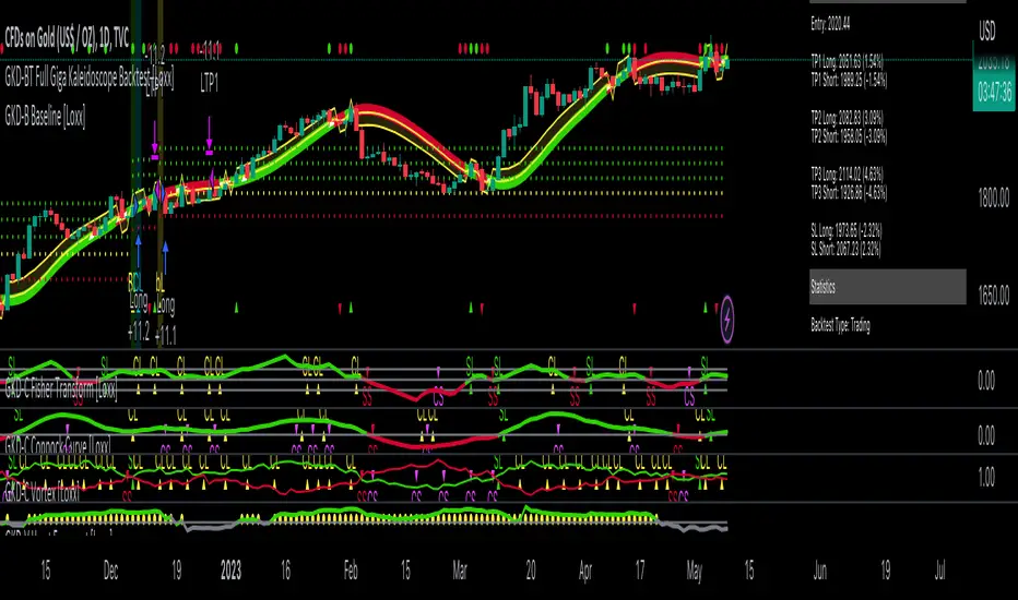
GKD-BT Full Giga Kaleidoscope Backtest [Loxx]Giga Kaleidoscope GKD-BT Full Giga Kaleidoscope Backtest is a Backtesting module included in Loxx's "Giga Kaleidoscope Modularized Trading System".
█ GKD-BT Full Giga Kaleidoscope Backtest
The Full Giga Kaleidoscope Backtest module enables users to backtest Full GKD Long and Short signals, allowing the creation of a comprehensive NNFX trading system consisting of two confirmation indicators, a baseline, a measure of volatility/volume, and continuations.
This module offers two types of backtests: Trading and Full. The Trading backtest allows users to evaluate individual Long and Short trades one by one. On the other hand, the Full backtest enables the analysis of Longs or Shorts separately by toggling between them in the settings, providing insights into the results for each signal type. The Trading backtest simulates actual trading conditions, while the Full backtest evaluates all signals regardless of their Long or Short nature.
Additionally, the backtest module allows testing with 1 to 3 take profits and 1 stop loss. The Trading backtest supports 1 to 3 take profits, while the Full backtest is limited to 1 take profit. The Trading backtest also includes a trailing take profit feature.
Regarding the percentage of trade removed at each take profit, the backtest module incorporates the following predefined values:
Take profit 1: 50% of the trade is removed.
Take profit 2: 25% of the trade is removed.
Take profit 3: 25% of the trade is removed.
Stop loss: 100% of the trade is removed.
After achieving each take profit, the stop loss level is adjusted accordingly. When take profit 1 is reached, the stop loss is moved to the entry point. Similarly, when take profit 2 is reached, the stop loss is shifted to take profit 1. The trailing take profit feature comes into effect after take profit 2 or take profit 3, depending on the number of take profits selected in the settings. The trailing take profit is always activated on the final take profit when 2 or more take profits are chosen.
The backtest module also provides the option to restrict testing to a specific date range, allowing for simulated forward testing using past data. Additionally, users can choose to display or hide a trading panel that provides relevant information about the backtest, statistics, and the current trade. It is also possible to activate alerts and toggle sections of the trading panel on or off. Historical take profit and stop loss levels are displayed as overlaid horizontal lines on the chart for reference.
To utilize this strategy, follow these steps:
1. GKD-B Baseline Import: Import the value "Input into NEW GKD-BT Backtest" from the GKD-B Baseline module into the GKD-BT Full Giga Kaleidoscope Backtest module setting named "Import GKD-B Baseline."
2. GKD-V Volatility/Volume Import: Import the value "Input into NEW GKD-BT Backtest" from the GKD-V Volatility/Volume module into the GKD-BT Full Giga Kaleidoscope Backtest module setting named "Import GKD-V Volatility/Volume."
3. Adjust the "Confirmation 1 Type" in the GKD-C Confirmation Indicator to "GKD New."
4. GKD-C Confirmation 1 Import: Import the value "Input into NEW GKD-BT Backtest" from the GKD-C Confirmation 1 module into the GKD-BT Full Giga Kaleidoscope Backtest module setting named "Import GKD-C Confirmation 1."
5. Adjust the "Confirmation 2 Type" in the GKD-C Confirmation 2 Indicator to "GKD New."
6. GKD-C Confirmation 2 Import: Import the value "Input into NEW GKD-BT Backtest" from the GKD-C Confirmation 2 module into the GKD-BT Full Giga Kaleidoscope Backtest module setting named "Import GKD-C Confirmation 2."
7. Adjust the "Confirmation Type" in the GKD-C Continuation Indicator to "GKD New."
8. GKD-C Continuation Import: Import the value "Input into NEW GKD-BT Backtest" from the GKD-C Continuation module into the GKD-BT Full Giga Kaleidoscope Backtest module setting named "Import GKD-C Confirmation."
The GKD system utilizes volatility-based take profits and stop losses, where each take profit and stop loss is calculated as a multiple of volatility. Users have the flexibility to adjust the multiplier values in the settings to suit their preferences.
In a future update, the Full Giga Kaleidoscope Backtest module will include the option to incorporate a GKD-E Exit indicator, completing the full trading strategy.
█ Full Giga Kaleidoscope Backtest Entries
Within this module, there are ten distinct types of entries available, which are outlined below:
Standard Entry
1-Candle Standard Entry
Baseline Entry
1-Candle Baseline Entry
Volatility/Volume Entry
1-Candle Volatility/Volume Entry
Confirmation 2 Entry
1-Candle Confirmation 2 Entry
PullBack Entry
Continuation Entry
Each of these entry types can generate either long or short signals, resulting in a total of 20 signal variations. The user has the flexibility to enable or disable specific entry types and choose which qualifying rules within each entry type are applied to price to determine the final long or short signal.
The following section provides an overview of the various entry types and their corresponding qualifying rules:
Standard Entry
1. GKD-C Confirmation gives signal
2. Baseline agrees
3. Price inside Goldie Locks Zone Minimum
4. Price inside Goldie Locks Zone Maximum
5. Confirmation 2 agrees
6. Volatility/Volume agrees
1-Candle Standard Entry
1a. GKD-C Confirmation gives signal
2a. Baseline agrees
3a. Price inside Goldie Locks Zone Minimum
4a. Price inside Goldie Locks Zone Maximum
Next Candle
1b. Price retraced
2b. Baseline agrees
3b. Confirmation 1 agrees
4b. Confirmation 2 agrees
5b. Volatility/Volume agrees
Baseline Entry
1. GKD-B Basline gives signal
2. Confirmation 1 agrees
3. Price inside Goldie Locks Zone Minimum
4. Price inside Goldie Locks Zone Maximum
5. Confirmation 2 agrees
6. Volatility/Volume agrees
7. Confirmation 1 signal was less than 'Maximum Allowable PSBC Bars Back' prior
1-Candle Baseline Entry
1a. GKD-B Baseline gives signal
2a. Confirmation 1 agrees
3a. Price inside Goldie Locks Zone Minimum
4a. Price inside Goldie Locks Zone Maximum
5a. Confirmation 1 signal was less than 'Maximum Allowable PSBC Bars Back' prior
Next Candle
1b. Price retraced
2b. Baseline agrees
3b. Confirmation 1 agrees
4b. Confirmation 2 agrees
5b. Volatility/Volume agrees
Volatility/Volume Entry
1. GKD-V Volatility/Volume gives signal
2. Confirmation 1 agrees
3. Price inside Goldie Locks Zone Minimum
4. Price inside Goldie Locks Zone Maximum
5. Confirmation 2 agrees
6. Baseline agrees
7. Confirmation 1 signal was less than 7 candles prior
1-Candle Volatility/Volume Entry
1a. GKD-V Volatility/Volume gives signal
2a. Confirmation 1 agrees
3a. Price inside Goldie Locks Zone Minimum
4a. Price inside Goldie Locks Zone Maximum
5a. Confirmation 1 signal was less than 'Maximum Allowable PSVVC Bars Back' prior
Next Candle
1b. Price retraced
2b. Volatility/Volume agrees
3b. Confirmation 1 agrees
4b. Confirmation 2 agrees
5b. Baseline agrees
Confirmation 2 Entry
1. GKD-C Confirmation 2 gives signal
2. Confirmation 1 agrees
3. Price inside Goldie Locks Zone Minimum
4. Price inside Goldie Locks Zone Maximum
5. Volatility/Volume agrees
6. Baseline agrees
7. Confirmation 1 signal was less than 7 candles prior
1-Candle Confirmation 2 Entry
1a. GKD-C Confirmation 2 gives signal
2a. Confirmation 1 agrees
3a. Price inside Goldie Locks Zone Minimum
4a. Price inside Goldie Locks Zone Maximum
5a. Confirmation 1 signal was less than 'Maximum Allowable PSC2C Bars Back' prior
Next Candle
1b. Price retraced
2b. Confirmation 2 agrees
3b. Confirmation 1 agrees
4b. Volatility/Volume agrees
5b. Baseline agrees
PullBack Entry
1a. GKD-B Baseline gives signal
2a. Confirmation 1 agrees
3a. Price is beyond 1.0x Volatility of Baseline
Next Candle
1b. Price inside Goldie Locks Zone Minimum
2b. Price inside Goldie Locks Zone Maximum
3b. Confirmation 1 agrees
4b. Confirmation 2 agrees
5b. Volatility/Volume agrees
Continuation Entry
1. Standard Entry, 1-Candle Standard Entry, Baseline Entry, 1-Candle Baseline Entry, Volatility/Volume Entry, 1-Candle Volatility/Volume Entry, Confirmation 2 Entry, 1-Candle Confirmation 2 Entry, or Pullback entry triggered previously
2. Baseline hasn't crossed since entry signal trigger
4. Confirmation 1 agrees
5. Baseline agrees
6. Confirmation 2 agrees
█ Volatility Types Included
This module includes 17 types of volatility:
Close-to-Close
Parkinson
Garman-Klass
Rogers-Satchell
Yang-Zhang
Garman-Klass-Yang-Zhang
Exponential Weighted Moving Average
Standard Deviation of Log Returns
Pseudo GARCH(2,2)
Average True Range
True Range Double
Standard Deviation
Adaptive Deviation
Median Absolute Deviation
Efficiency-Ratio Adaptive ATR
Mean Absolute Deviation
Static Percent
Close-to-Close
Close-to-Close volatility is a classic and widely used volatility measure, sometimes referred to as historical volatility.
Volatility is an indicator of the speed of a stock price change. A stock with high volatility is one where the price changes rapidly and with a larger amplitude. The more volatile a stock is, the riskier it is.
Close-to-close historical volatility is calculated using only a stock's closing prices. It is the simplest volatility estimator. However, in many cases, it is not precise enough. Stock prices could jump significantly during a trading session and return to the opening value at the end. That means that a considerable amount of price information is not taken into account by close-to-close volatility.
Despite its drawbacks, Close-to-Close volatility is still useful in cases where the instrument doesn't have intraday prices. For example, mutual funds calculate their net asset values daily or weekly, and thus their prices are not suitable for more sophisticated volatility estimators.
Parkinson
Parkinson volatility is a volatility measure that uses the stock’s high and low price of the day.
The main difference between regular volatility and Parkinson volatility is that the latter uses high and low prices for a day, rather than only the closing price. This is useful as close-to-close prices could show little difference while large price movements could have occurred during the day. Thus, Parkinson's volatility is considered more precise and requires less data for calculation than close-to-close volatility.
One drawback of this estimator is that it doesn't take into account price movements after the market closes. Hence, it systematically undervalues volatility. This drawback is addressed in the Garman-Klass volatility estimator.
Garman-Klass
Garman-Klass is a volatility estimator that incorporates open, low, high, and close prices of a security.
Garman-Klass volatility extends Parkinson's volatility by taking into account the opening and closing prices. As markets are most active during the opening and closing of a trading session, it makes volatility estimation more accurate.
Garman and Klass also assumed that the process of price change follows a continuous diffusion process (Geometric Brownian motion). However, this assumption has several drawbacks. The method is not robust for opening jumps in price and trend movements.
Despite its drawbacks, the Garman-Klass estimator is still more effective than the basic formula since it takes into account not only the price at the beginning and end of the time interval but also intraday price extremes.
Researchers Rogers and Satchell have proposed a more efficient method for assessing historical volatility that takes into account price trends. See Rogers-Satchell Volatility for more detail.
Rogers-Satchell
Rogers-Satchell is an estimator for measuring the volatility of securities with an average return not equal to zero.
Unlike Parkinson and Garman-Klass estimators, Rogers-Satchell incorporates a drift term (mean return not equal to zero). As a result, it provides better volatility estimation when the underlying is trending.
The main disadvantage of this method is that it does not take into account price movements between trading sessions. This leads to an underestimation of volatility since price jumps periodically occur in the market precisely at the moments between sessions.
A more comprehensive estimator that also considers the gaps between sessions was developed based on the Rogers-Satchel formula in the 2000s by Yang-Zhang. See Yang Zhang Volatility for more detail.
Yang-Zhang
Yang Zhang is a historical volatility estimator that handles both opening jumps and the drift and has a minimum estimation error.
Yang-Zhang volatility can be thought of as a combination of the overnight (close-to-open volatility) and a weighted average of the Rogers-Satchell volatility and the day’s open-to-close volatility. It is considered to be 14 times more efficient than the close-to-close estimator.
Garman-Klass-Yang-Zhang
Garman-Klass-Yang-Zhang (GKYZ) volatility estimator incorporates the returns of open, high, low, and closing prices in its calculation.
GKYZ volatility estimator takes into account overnight jumps but not the trend, i.e., it assumes that the underlying asset follows a Geometric Brownian Motion (GBM) process with zero drift. Therefore, the GKYZ volatility estimator tends to overestimate the volatility when the drift is different from zero. However, for a GBM process, this estimator is eight times more efficient than the close-to-close volatility estimator.
Exponential Weighted Moving Average
The Exponentially Weighted Moving Average (EWMA) is a quantitative or statistical measure used to model or describe a time series. The EWMA is widely used in finance, with the main applications being technical analysis and volatility modeling.
The moving average is designed such that older observations are given lower weights. The weights decrease exponentially as the data point gets older – hence the name exponentially weighted.
The only decision a user of the EWMA must make is the parameter lambda. The parameter decides how important the current observation is in the calculation of the EWMA. The higher the value of lambda, the more closely the EWMA tracks the original time series.
Standard Deviation of Log Returns
This is the simplest calculation of volatility. It's the standard deviation of ln(close/close(1)).
Pseudo GARCH(2,2)
This is calculated using a short- and long-run mean of variance multiplied by ?.
?avg(var;M) + (1 ? ?) avg(var;N) = 2?var/(M+1-(M-1)L) + 2(1-?)var/(M+1-(M-1)L)
Solving for ? can be done by minimizing the mean squared error of estimation; that is, regressing L^-1var - avg(var; N) against avg(var; M) - avg(var; N) and using the resulting beta estimate as ?.
Average True Range
The average true range (ATR) is a technical analysis indicator, introduced by market technician J. Welles Wilder Jr. in his book New Concepts in Technical Trading Systems, that measures market volatility by decomposing the entire range of an asset price for that period.
The true range indicator is taken as the greatest of the following: current high less the current low; the absolute value of the current high less the previous close; and the absolute value of the current low less the previous close. The ATR is then a moving average, generally using 14 days, of the true ranges.
True Range Double
A special case of ATR that attempts to correct for volatility skew.
Standard Deviation
Standard deviation is a statistic that measures the dispersion of a dataset relative to its mean and is calculated as the square root of the variance. The standard deviation is calculated as the square root of variance by determining each data point's deviation relative to the mean. If the data points are further from the mean, there is a higher deviation within the data set; thus, the more spread out the data, the higher the standard deviation.
Adaptive Deviation
By definition, the Standard Deviation (STD, also represented by the Greek letter sigma ? or the Latin letter s) is a measure that is used to quantify the amount of variation or dispersion of a set of data values. In technical analysis, we usually use it to measure the level of current volatility.
Standard Deviation is based on Simple Moving Average calculation for mean value. This version of standard deviation uses the properties of EMA to calculate what can be called a new type of deviation, and since it is based on EMA, we can call it EMA deviation. Additionally, Perry Kaufman's efficiency ratio is used to make it adaptive (since all EMA type calculations are nearly perfect for adapting).
The difference when compared to the standard is significant--not just because of EMA usage, but the efficiency ratio makes it a "bit more logical" in very volatile market conditions.
Median Absolute Deviation
The median absolute deviation is a measure of statistical dispersion. Moreover, the MAD is a robust statistic, being more resilient to outliers in a data set than the standard deviation. In the standard deviation, the distances from the mean are squared, so large deviations are weighted more heavily, and thus outliers can heavily influence it. In the MAD, the deviations of a small number of outliers are irrelevant.
Because the MAD is a more robust estimator of scale than the sample variance or standard deviation, it works better with distributions without a mean or variance, such as the Cauchy distribution.
Efficiency-Ratio Adaptive ATR
Average True Range (ATR) is a widely used indicator for many occasions in technical analysis. It is calculated as the RMA of the true range. This version adds a "twist": it uses Perry Kaufman's Efficiency Ratio to calculate adaptive true range.
Mean Absolute Deviation
The mean absolute deviation (MAD) is a measure of variability that indicates the average distance between observations and their mean. MAD uses the original units of the data, which simplifies interpretation. Larger values signify that the data points spread out further from the average. Conversely, lower values correspond to data points bunching closer to it. The mean absolute deviation is also known as the mean deviation and average absolute deviation.
This definition of the mean absolute deviation sounds similar to the standard deviation (SD). While both measure variability, they have different calculations. In recent years, some proponents of MAD have suggested that it replace the SD as the primary measure because it is a simpler concept that better fits real life.
Static Percent
Static Percent allows the user to insert their own constant percent that will then be used to create take profits and stoploss
█ Giga Kaleidoscope Modularized Trading System
Core components of an NNFX algorithmic trading strategy
The NNFX algorithm is built on the principles of trend, momentum, and volatility. There are six core components in the NNFX trading algorithm:
1. Volatility - price volatility; e.g., Average True Range, True Range Double, Close-to-Close, etc.
2. Baseline - a moving average to identify price trend
3. Confirmation 1 - a technical indicator used to identify trends
4. Confirmation 2 - a technical indicator used to identify trends
5. Continuation - a technical indicator used to identify trends
6. Volatility/Volume - a technical indicator used to identify volatility/volume breakouts/breakdown
7. Exit - a technical indicator used to determine when a trend is exhausted
What is Volatility in the NNFX trading system?
In the NNFX (No Nonsense Forex) trading system, ATR (Average True Range) is typically used to measure the volatility of an asset. It is used as a part of the system to help determine the appropriate stop loss and take profit levels for a trade. ATR is calculated by taking the average of the true range values over a specified period.
True range is calculated as the maximum of the following values:
-Current high minus the current low
-Absolute value of the current high minus the previous close
-Absolute value of the current low minus the previous close
ATR is a dynamic indicator that changes with changes in volatility. As volatility increases, the value of ATR increases, and as volatility decreases, the value of ATR decreases. By using ATR in NNFX system, traders can adjust their stop loss and take profit levels according to the volatility of the asset being traded. This helps to ensure that the trade is given enough room to move, while also minimizing potential losses.
Other types of volatility include True Range Double (TRD), Close-to-Close, and Garman-Klass
What is a Baseline indicator?
The baseline is essentially a moving average, and is used to determine the overall direction of the market.
The baseline in the NNFX system is used to filter out trades that are not in line with the long-term trend of the market. The baseline is plotted on the chart along with other indicators, such as the Moving Average (MA), the Relative Strength Index (RSI), and the Average True Range (ATR).
Trades are only taken when the price is in the same direction as the baseline. For example, if the baseline is sloping upwards, only long trades are taken, and if the baseline is sloping downwards, only short trades are taken. This approach helps to ensure that trades are in line with the overall trend of the market, and reduces the risk of entering trades that are likely to fail.
By using a baseline in the NNFX system, traders can have a clear reference point for determining the overall trend of the market, and can make more informed trading decisions. The baseline helps to filter out noise and false signals, and ensures that trades are taken in the direction of the long-term trend.
What is a Confirmation indicator?
Confirmation indicators are technical indicators that are used to confirm the signals generated by primary indicators. Primary indicators are the core indicators used in the NNFX system, such as the Average True Range (ATR), the Moving Average (MA), and the Relative Strength Index (RSI).
The purpose of the confirmation indicators is to reduce false signals and improve the accuracy of the trading system. They are designed to confirm the signals generated by the primary indicators by providing additional information about the strength and direction of the trend.
Some examples of confirmation indicators that may be used in the NNFX system include the Bollinger Bands, the MACD (Moving Average Convergence Divergence), and the MACD Oscillator. These indicators can provide information about the volatility, momentum, and trend strength of the market, and can be used to confirm the signals generated by the primary indicators.
In the NNFX system, confirmation indicators are used in combination with primary indicators and other filters to create a trading system that is robust and reliable. By using multiple indicators to confirm trading signals, the system aims to reduce the risk of false signals and improve the overall profitability of the trades.
What is a Continuation indicator?
In the NNFX (No Nonsense Forex) trading system, a continuation indicator is a technical indicator that is used to confirm a current trend and predict that the trend is likely to continue in the same direction. A continuation indicator is typically used in conjunction with other indicators in the system, such as a baseline indicator, to provide a comprehensive trading strategy.
What is a Volatility/Volume indicator?
Volume indicators, such as the On Balance Volume (OBV), the Chaikin Money Flow (CMF), or the Volume Price Trend (VPT), are used to measure the amount of buying and selling activity in a market. They are based on the trading volume of the market, and can provide information about the strength of the trend. In the NNFX system, volume indicators are used to confirm trading signals generated by the Moving Average and the Relative Strength Index. Volatility indicators include Average Direction Index, Waddah Attar, and Volatility Ratio. In the NNFX trading system, volatility is a proxy for volume and vice versa.
By using volume indicators as confirmation tools, the NNFX trading system aims to reduce the risk of false signals and improve the overall profitability of trades. These indicators can provide additional information about the market that is not captured by the primary indicators, and can help traders to make more informed trading decisions. In addition, volume indicators can be used to identify potential changes in market trends and to confirm the strength of price movements.
What is an Exit indicator?
The exit indicator is used in conjunction with other indicators in the system, such as the Moving Average (MA), the Relative Strength Index (RSI), and the Average True Range (ATR), to provide a comprehensive trading strategy.
The exit indicator in the NNFX system can be any technical indicator that is deemed effective at identifying optimal exit points. Examples of exit indicators that are commonly used include the Parabolic SAR, the Average Directional Index (ADX), and the Chandelier Exit.
The purpose of the exit indicator is to identify when a trend is likely to reverse or when the market conditions have changed, signaling the need to exit a trade. By using an exit indicator, traders can manage their risk and prevent significant losses.
In the NNFX system, the exit indicator is used in conjunction with a stop loss and a take profit order to maximize profits and minimize losses. The stop loss order is used to limit the amount of loss that can be incurred if the trade goes against the trader, while the take profit order is used to lock in profits when the trade is moving in the trader's favor.
Overall, the use of an exit indicator in the NNFX trading system is an important component of a comprehensive trading strategy. It allows traders to manage their risk effectively and improve the profitability of their trades by exiting at the right time.
How does Loxx's GKD (Giga Kaleidoscope Modularized Trading System) implement the NNFX algorithm outlined above?
Loxx's GKD v2.0 system has five types of modules (indicators/strategies). These modules are:
1. GKD-BT - Backtesting module (Volatility, Number 1 in the NNFX algorithm)
2. GKD-B - Baseline module (Baseline and Volatility/Volume, Numbers 1 and 2 in the NNFX algorithm)
3. GKD-C - Confirmation 1/2 and Continuation module (Confirmation 1/2 and Continuation, Numbers 3, 4, and 5 in the NNFX algorithm)
4. GKD-V - Volatility/Volume module (Confirmation 1/2, Number 6 in the NNFX algorithm)
5. GKD-E - Exit module (Exit, Number 7 in the NNFX algorithm)
(additional module types will added in future releases)
Each module interacts with every module by passing data to A backtest module wherein the various components of the GKD system are combined to create a trading signal.
That is, the Baseline indicator passes its data to Volatility/Volume. The Volatility/Volume indicator passes its values to the Confirmation 1 indicator. The Confirmation 1 indicator passes its values to the Confirmation 2 indicator. The Confirmation 2 indicator passes its values to the Continuation indicator. The Continuation indicator passes its values to the Exit indicator, and finally, the Exit indicator passes its values to the Backtest strategy.
This chaining of indicators requires that each module conform to Loxx's GKD protocol, therefore allowing for the testing of every possible combination of technical indicators that make up the six components of the NNFX algorithm.
What does the application of the GKD trading system look like?
Example trading system:
Backtest: Full Giga Kaleidoscope Backtest as shown on the chart above
Baseline: Hull Moving Average as shown on the chart above
Volatility/Volume: Hurst Exponent as shown on the chart above
Confirmation 1: Vorext as shown on the chart above
Confirmation 2: Coppock Curve as shown on the chart above
Continuation: Fisher Transform as shown on the chart above
Exit: Rex Oscillator
Each GKD indicator is denoted with a module identifier of either: GKD-BT, GKD-B, GKD-C, GKD-V, or GKD-E. This allows traders to understand to which module each indicator belongs and where each indicator fits into the GKD system.
GKD-BT Solo Confirmation Super Complex Backtest [Loxx]Giga Kaleidoscope GKD-BT Solo Confirmation Super Complex Backtest is a Backtesting module included in Loxx's "Giga Kaleidoscope Modularized Trading System".
█ GKD-BT Solo Confirmation Super Complex Backtest
The Solo Confirmation Super Complex Backtest module allows users to perform backtesting on Full GKD Long and Short signals using GKD-C confirmation indicators. These signals are further refined by GKD-B Baseline and GKD-V Volatility/Volume indicators and augmented by an additional GKD-C Confirmation indicator acting as a Continuation indicator. This module serves as a comprehensive tool that falls just below a Full GKD trading system. The key difference is that the GKD-BT Solo Confirmation Super Complex utilizes a single GKD-C Confirmation indicator, while the Full GKD system employs two GKD-C Confirmation indicators. Both the Solo Confirmation Super Complex and the Full GKD systems incorporate an extra GKD-C Confirmation indicator to identify Continuation signals, which provide both longs and shorts on developing trends following an initial trend change.
This module encompasses two types of backtests: Trading and Full. The Trading backtest permits users to evaluate individual trades, whether Long or Short, one at a time. Conversely, the Full backtest allows users to analyze either Longs or Shorts separately by toggling between them in the settings, enabling the examination of results for each signal type. The Trading backtest emulates actual trading conditions, while the Full backtest assesses all signals, regardless of being Long or Short.
Additionally, this backtest module provides the option to test the core GKD-C Confirmation and GKD-C Continuation indicators with 1 to 3 take profits and 1 stop loss. The Trading backtest allows for the use of 1 to 3 take profits, while the Full backtest is limited to 1 take profit. The Trading backtest also offers the capability to apply a trailing take profit.
In terms of the percentage of trade removed at each take profit, this backtest module has the following hardcoded values:
Take profit 1: 50% of the trade is removed.
Take profit 2: 25% of the trade is removed.
Take profit 3: 25% of the trade is removed.
Stop loss: 100% of the trade is removed.
After each take profit is achieved, the stop loss level is adjusted. When take profit 1 is reached, the stop loss is moved to the entry point. Similarly, when take profit 2 is reached, the stop loss is shifted to take profit 1. The trailing take profit feature comes into play after take profit 2 or take profit 3, depending on the number of take profits selected in the settings. The trailing take profit is always activated on the final take profit when 2 or more take profits are chosen.
The backtest module also offers the capability to restrict by a specific date range, allowing for simulated forward testing based on past data. Additionally, users have the option to display or hide a trading panel that provides relevant information about the backtest, statistics, and the current trade. It is also possible to activate alerts and toggle sections of the trading panel on or off. On the chart, historical take profit and stop loss levels are represented by horizontal lines overlaid for reference.
To utilize this strategy, follow these steps:
1. GKD-B Baseline Import: Import the value "Input into NEW GKD-BT Backtest" from the GKD-B Baseline module into the GKD-BT Solo Confirmation Super Complex Backtest module setting named "Import GKD-B Baseline."
2. GKD-V Volatility/Volume Import: Import the value "Input into NEW GKD-BT Backtest" from the GKD-V Volatility/Volume module into the GKD-BT Solo Confirmation Super Complex Backtest module setting named "Import GKD-V Volatility/Volume."
3. Adjust the "Confirmation Type" in the GKD-C Confirmation Indicator to "GKD New."
4. GKD-C Confirmation Import: Import the value "Input into NEW GKD-BT Backtest" from the GKD-C Confirmation module into the GKD-BT Solo Confirmation Super Complex Backtest module setting named "Import GKD-C Confirmation."
5. Adjust the "Confirmation Type" in the GKD-C Continuation Indicator to "GKD New."
6. GKD-C Continuation Import: Import the value "Input into NEW GKD-BT Backtest" from the GKD-C Continuation module into the GKD-BT Solo Confirmation Super Complex Backtest module setting named "Import GKD-C Continuation."
The GKD system utilizes volatility-based take profits and stop losses. Each take profit and stop loss is calculated as a multiple of volatility. Users can also adjust the multiplier values in the settings.
In a future update, the option to include a GKD-E Exit indicator will be added to this module to complete a full trading strategy.
█ Solo Confirmation Super Complex Backtest Entries
Within this module, there are eight distinct types of entries available, which are outlined below:
Standard Entry
1-Candle Standard Entry
Baseline Entry
1-Candle Baseline Entry
Volatility/Volume Entry
1-Candle Volatility/Volume Entry
PullBack Entry
Continuation Entry
Each of these entry types can generate either long or short signals, resulting in a total of 16 signal variations. The user has the flexibility to enable or disable specific entry types and choose which qualifying rules within each entry type are applied to price to determine the final long or short signal. You'll notice that these signals are different form the core GKD signals mentioned towards the end of this description. Signals from the GKD-BT Solo Confirmation Super Complex Backtest are modifided to add additional qualifications to make your finalized trading strategy more dynamic and robust.
The following section provides an overview of the various entry types and their corresponding qualifying rules:
Standard Entry
1. GKD-C Confirmation gives signal
2. Baseline agrees
3. Price inside Goldie Locks Zone Minimum
4. Price inside Goldie Locks Zone Maximum
5. Volatility/Volume agrees
1-Candle Standard Entry
1a. GKD-C Confirmation gives signal
2a. Baseline agrees
3a. Price inside Goldie Locks Zone Minimum
4a. Price inside Goldie Locks Zone Maximum
Next Candle:
1b. Price retraced
2b. Baseline agrees
3b. Confirmation 1 agrees
4b. Volatility/Volume agrees
Baseline Entry
1. GKD-B Basline gives signal
2. Confirmation 1 agrees
3. Price inside Goldie Locks Zone Minimum
4. Price inside Goldie Locks Zone Maximum
5. Volatility/Volume agrees
6. Confirmation 1 signal was less than 'Maximum Allowable PSBC Bars Back' prior
1-Candle Baseline Entry
1a. GKD-B Basline gives signal
2a. Confirmation 1 agrees
3a. Price inside Goldie Locks Zone Minimum
4a. Price inside Goldie Locks Zone Maximum
5a. Confirmation 1 signal was less than 'Maximum Allowable PSBC Bars Back' prior
Next Candle:
1b. Price retraced
2b. Baseline agrees
3b. Confirmation 1 agrees
4b. Volatility/Volume agrees
Volatility/Volume Entry
1. GKD-V Volatility/Volume gives signal
2. Confirmation 1 agrees
3. Price inside Goldie Locks Zone Minimum
4. Price inside Goldie Locks Zone Maximum
5. Baseline agrees
6. Confirmation 1 signal was less than 7 candles prior
1-Candle Volatility/Volume Entry
1a. GKD-V Volatility/Volume gives signal
2a. Confirmation 1 agrees
3a. Price inside Goldie Locks Zone Minimum
4a. Price inside Goldie Locks Zone Maximum
5a. Confirmation 1 signal was less than 'Maximum Allowable PSVVC Bars Back' prior
Next Candle:
1b. Price retraced
2b. Volatility/Volume agrees
3b. Confirmation 1 agrees
4b. Baseline agrees
PullBack Entry
1a. GKD-B Baseline gives signal
2a. Confirmation 1 agrees
3a. Price is beyond 1.0x Volatility of Baseline
Next Candle:
1b. Price inside Goldie Locks Zone Minimum
2b. Price inside Goldie Locks Zone Maximum
3b. Confirmation 1 agrees
4b. Volatility/Volume agrees
Continuation Entry
1. Standard Entry, 1-Candle Standard Entry, Baseline Entry, 1-Candle Baseline Entry, Volatility/Volume Entry, 1-Candle Volatility/Volume Entry, or Pullback entry triggered previously
2. Baseline hasn't crossed since entry signal trigger
4. Confirmation 1 agrees
5. Baseline agrees
█ Volatility Types Included
This module includes 17 types of volatility:
Close-to-Close
Parkinson
Garman-Klass
Rogers-Satchell
Yang-Zhang
Garman-Klass-Yang-Zhang
Exponential Weighted Moving Average
Standard Deviation of Log Returns
Pseudo GARCH(2,2)
Average True Range
True Range Double
Standard Deviation
Adaptive Deviation
Median Absolute Deviation
Efficiency-Ratio Adaptive ATR
Mean Absolute Deviation
Static Percent
Close-to-Close
Close-to-Close volatility is a classic and widely used volatility measure, sometimes referred to as historical volatility.
Volatility is an indicator of the speed of a stock price change. A stock with high volatility is one where the price changes rapidly and with a larger amplitude. The more volatile a stock is, the riskier it is.
Close-to-close historical volatility is calculated using only a stock's closing prices. It is the simplest volatility estimator. However, in many cases, it is not precise enough. Stock prices could jump significantly during a trading session and return to the opening value at the end. That means that a considerable amount of price information is not taken into account by close-to-close volatility.
Despite its drawbacks, Close-to-Close volatility is still useful in cases where the instrument doesn't have intraday prices. For example, mutual funds calculate their net asset values daily or weekly, and thus their prices are not suitable for more sophisticated volatility estimators.
Parkinson
Parkinson volatility is a volatility measure that uses the stock’s high and low price of the day.
The main difference between regular volatility and Parkinson volatility is that the latter uses high and low prices for a day, rather than only the closing price. This is useful as close-to-close prices could show little difference while large price movements could have occurred during the day. Thus, Parkinson's volatility is considered more precise and requires less data for calculation than close-to-close volatility.
One drawback of this estimator is that it doesn't take into account price movements after the market closes. Hence, it systematically undervalues volatility. This drawback is addressed in the Garman-Klass volatility estimator.
Garman-Klass
Garman-Klass is a volatility estimator that incorporates open, low, high, and close prices of a security.
Garman-Klass volatility extends Parkinson's volatility by taking into account the opening and closing prices. As markets are most active during the opening and closing of a trading session, it makes volatility estimation more accurate.
Garman and Klass also assumed that the process of price change follows a continuous diffusion process (Geometric Brownian motion). However, this assumption has several drawbacks. The method is not robust for opening jumps in price and trend movements.
Despite its drawbacks, the Garman-Klass estimator is still more effective than the basic formula since it takes into account not only the price at the beginning and end of the time interval but also intraday price extremes.
Researchers Rogers and Satchell have proposed a more efficient method for assessing historical volatility that takes into account price trends. See Rogers-Satchell Volatility for more detail.
Rogers-Satchell
Rogers-Satchell is an estimator for measuring the volatility of securities with an average return not equal to zero.
Unlike Parkinson and Garman-Klass estimators, Rogers-Satchell incorporates a drift term (mean return not equal to zero). As a result, it provides better volatility estimation when the underlying is trending.
The main disadvantage of this method is that it does not take into account price movements between trading sessions. This leads to an underestimation of volatility since price jumps periodically occur in the market precisely at the moments between sessions.
A more comprehensive estimator that also considers the gaps between sessions was developed based on the Rogers-Satchel formula in the 2000s by Yang-Zhang. See Yang Zhang Volatility for more detail.
Yang-Zhang
Yang Zhang is a historical volatility estimator that handles both opening jumps and the drift and has a minimum estimation error.
Yang-Zhang volatility can be thought of as a combination of the overnight (close-to-open volatility) and a weighted average of the Rogers-Satchell volatility and the day’s open-to-close volatility. It is considered to be 14 times more efficient than the close-to-close estimator.
Garman-Klass-Yang-Zhang
Garman-Klass-Yang-Zhang (GKYZ) volatility estimator incorporates the returns of open, high, low, and closing prices in its calculation.
GKYZ volatility estimator takes into account overnight jumps but not the trend, i.e., it assumes that the underlying asset follows a Geometric Brownian Motion (GBM) process with zero drift. Therefore, the GKYZ volatility estimator tends to overestimate the volatility when the drift is different from zero. However, for a GBM process, this estimator is eight times more efficient than the close-to-close volatility estimator.
Exponential Weighted Moving Average
The Exponentially Weighted Moving Average (EWMA) is a quantitative or statistical measure used to model or describe a time series. The EWMA is widely used in finance, with the main applications being technical analysis and volatility modeling.
The moving average is designed such that older observations are given lower weights. The weights decrease exponentially as the data point gets older – hence the name exponentially weighted.
The only decision a user of the EWMA must make is the parameter lambda. The parameter decides how important the current observation is in the calculation of the EWMA. The higher the value of lambda, the more closely the EWMA tracks the original time series.
Standard Deviation of Log Returns
This is the simplest calculation of volatility. It's the standard deviation of ln(close/close(1)).
Pseudo GARCH(2,2)
This is calculated using a short- and long-run mean of variance multiplied by ?.
?avg(var;M) + (1 ? ?) avg(var;N) = 2?var/(M+1-(M-1)L) + 2(1-?)var/(M+1-(M-1)L)
Solving for ? can be done by minimizing the mean squared error of estimation; that is, regressing L^-1var - avg(var; N) against avg(var; M) - avg(var; N) and using the resulting beta estimate as ?.
Average True Range
The average true range (ATR) is a technical analysis indicator, introduced by market technician J. Welles Wilder Jr. in his book New Concepts in Technical Trading Systems, that measures market volatility by decomposing the entire range of an asset price for that period.
The true range indicator is taken as the greatest of the following: current high less the current low; the absolute value of the current high less the previous close; and the absolute value of the current low less the previous close. The ATR is then a moving average, generally using 14 days, of the true ranges.
True Range Double
A special case of ATR that attempts to correct for volatility skew.
Standard Deviation
Standard deviation is a statistic that measures the dispersion of a dataset relative to its mean and is calculated as the square root of the variance. The standard deviation is calculated as the square root of variance by determining each data point's deviation relative to the mean. If the data points are further from the mean, there is a higher deviation within the data set; thus, the more spread out the data, the higher the standard deviation.
Adaptive Deviation
By definition, the Standard Deviation (STD, also represented by the Greek letter sigma ? or the Latin letter s) is a measure that is used to quantify the amount of variation or dispersion of a set of data values. In technical analysis, we usually use it to measure the level of current volatility.
Standard Deviation is based on Simple Moving Average calculation for mean value. This version of standard deviation uses the properties of EMA to calculate what can be called a new type of deviation, and since it is based on EMA, we can call it EMA deviation. Additionally, Perry Kaufman's efficiency ratio is used to make it adaptive (since all EMA type calculations are nearly perfect for adapting).
The difference when compared to the standard is significant--not just because of EMA usage, but the efficiency ratio makes it a "bit more logical" in very volatile market conditions.
Median Absolute Deviation
The median absolute deviation is a measure of statistical dispersion. Moreover, the MAD is a robust statistic, being more resilient to outliers in a data set than the standard deviation. In the standard deviation, the distances from the mean are squared, so large deviations are weighted more heavily, and thus outliers can heavily influence it. In the MAD, the deviations of a small number of outliers are irrelevant.
Because the MAD is a more robust estimator of scale than the sample variance or standard deviation, it works better with distributions without a mean or variance, such as the Cauchy distribution.
Efficiency-Ratio Adaptive ATR
Average True Range (ATR) is a widely used indicator for many occasions in technical analysis. It is calculated as the RMA of the true range. This version adds a "twist": it uses Perry Kaufman's Efficiency Ratio to calculate adaptive true range.
Mean Absolute Deviation
The mean absolute deviation (MAD) is a measure of variability that indicates the average distance between observations and their mean. MAD uses the original units of the data, which simplifies interpretation. Larger values signify that the data points spread out further from the average. Conversely, lower values correspond to data points bunching closer to it. The mean absolute deviation is also known as the mean deviation and average absolute deviation.
This definition of the mean absolute deviation sounds similar to the standard deviation (SD). While both measure variability, they have different calculations. In recent years, some proponents of MAD have suggested that it replace the SD as the primary measure because it is a simpler concept that better fits real life.
Static Percent
Static Percent allows the user to insert their own constant percent that will then be used to create take profits and stoploss
█ Giga Kaleidoscope Modularized Trading System
Core components of an NNFX algorithmic trading strategy
The NNFX algorithm is built on the principles of trend, momentum, and volatility. There are six core components in the NNFX trading algorithm:
1. Volatility - price volatility; e.g., Average True Range, True Range Double, Close-to-Close, etc.
2. Baseline - a moving average to identify price trend
3. Confirmation 1 - a technical indicator used to identify trends
4. Confirmation 2 - a technical indicator used to identify trends
5. Continuation - a technical indicator used to identify trends
6. Volatility/Volume - a technical indicator used to identify volatility/volume breakouts/breakdown
7. Exit - a technical indicator used to determine when a trend is exhausted
What is Volatility in the NNFX trading system?
In the NNFX (No Nonsense Forex) trading system, ATR (Average True Range) is typically used to measure the volatility of an asset. It is used as a part of the system to help determine the appropriate stop loss and take profit levels for a trade. ATR is calculated by taking the average of the true range values over a specified period.
True range is calculated as the maximum of the following values:
-Current high minus the current low
-Absolute value of the current high minus the previous close
-Absolute value of the current low minus the previous close
ATR is a dynamic indicator that changes with changes in volatility. As volatility increases, the value of ATR increases, and as volatility decreases, the value of ATR decreases. By using ATR in NNFX system, traders can adjust their stop loss and take profit levels according to the volatility of the asset being traded. This helps to ensure that the trade is given enough room to move, while also minimizing potential losses.
Other types of volatility include True Range Double (TRD), Close-to-Close, and Garman-Klass
What is a Baseline indicator?
The baseline is essentially a moving average, and is used to determine the overall direction of the market.
The baseline in the NNFX system is used to filter out trades that are not in line with the long-term trend of the market. The baseline is plotted on the chart along with other indicators, such as the Moving Average (MA), the Relative Strength Index (RSI), and the Average True Range (ATR).
Trades are only taken when the price is in the same direction as the baseline. For example, if the baseline is sloping upwards, only long trades are taken, and if the baseline is sloping downwards, only short trades are taken. This approach helps to ensure that trades are in line with the overall trend of the market, and reduces the risk of entering trades that are likely to fail.
By using a baseline in the NNFX system, traders can have a clear reference point for determining the overall trend of the market, and can make more informed trading decisions. The baseline helps to filter out noise and false signals, and ensures that trades are taken in the direction of the long-term trend.
What is a Confirmation indicator?
Confirmation indicators are technical indicators that are used to confirm the signals generated by primary indicators. Primary indicators are the core indicators used in the NNFX system, such as the Average True Range (ATR), the Moving Average (MA), and the Relative Strength Index (RSI).
The purpose of the confirmation indicators is to reduce false signals and improve the accuracy of the trading system. They are designed to confirm the signals generated by the primary indicators by providing additional information about the strength and direction of the trend.
Some examples of confirmation indicators that may be used in the NNFX system include the Bollinger Bands, the MACD (Moving Average Convergence Divergence), and the MACD Oscillator. These indicators can provide information about the volatility, momentum, and trend strength of the market, and can be used to confirm the signals generated by the primary indicators.
In the NNFX system, confirmation indicators are used in combination with primary indicators and other filters to create a trading system that is robust and reliable. By using multiple indicators to confirm trading signals, the system aims to reduce the risk of false signals and improve the overall profitability of the trades.
What is a Continuation indicator?
In the NNFX (No Nonsense Forex) trading system, a continuation indicator is a technical indicator that is used to confirm a current trend and predict that the trend is likely to continue in the same direction. A continuation indicator is typically used in conjunction with other indicators in the system, such as a baseline indicator, to provide a comprehensive trading strategy.
What is a Volatility/Volume indicator?
Volume indicators, such as the On Balance Volume (OBV), the Chaikin Money Flow (CMF), or the Volume Price Trend (VPT), are used to measure the amount of buying and selling activity in a market. They are based on the trading volume of the market, and can provide information about the strength of the trend. In the NNFX system, volume indicators are used to confirm trading signals generated by the Moving Average and the Relative Strength Index. Volatility indicators include Average Direction Index, Waddah Attar, and Volatility Ratio. In the NNFX trading system, volatility is a proxy for volume and vice versa.
By using volume indicators as confirmation tools, the NNFX trading system aims to reduce the risk of false signals and improve the overall profitability of trades. These indicators can provide additional information about the market that is not captured by the primary indicators, and can help traders to make more informed trading decisions. In addition, volume indicators can be used to identify potential changes in market trends and to confirm the strength of price movements.
What is an Exit indicator?
The exit indicator is used in conjunction with other indicators in the system, such as the Moving Average (MA), the Relative Strength Index (RSI), and the Average True Range (ATR), to provide a comprehensive trading strategy.
The exit indicator in the NNFX system can be any technical indicator that is deemed effective at identifying optimal exit points. Examples of exit indicators that are commonly used include the Parabolic SAR, the Average Directional Index (ADX), and the Chandelier Exit.
The purpose of the exit indicator is to identify when a trend is likely to reverse or when the market conditions have changed, signaling the need to exit a trade. By using an exit indicator, traders can manage their risk and prevent significant losses.
In the NNFX system, the exit indicator is used in conjunction with a stop loss and a take profit order to maximize profits and minimize losses. The stop loss order is used to limit the amount of loss that can be incurred if the trade goes against the trader, while the take profit order is used to lock in profits when the trade is moving in the trader's favor.
Overall, the use of an exit indicator in the NNFX trading system is an important component of a comprehensive trading strategy. It allows traders to manage their risk effectively and improve the profitability of their trades by exiting at the right time.
How does Loxx's GKD (Giga Kaleidoscope Modularized Trading System) implement the NNFX algorithm outlined above?
Loxx's GKD v2.0 system has five types of modules (indicators/strategies). These modules are:
1. GKD-BT - Backtesting module (Volatility, Number 1 in the NNFX algorithm)
2. GKD-B - Baseline module (Baseline and Volatility/Volume, Numbers 1 and 2 in the NNFX algorithm)
3. GKD-C - Confirmation 1/2 and Continuation module (Confirmation 1/2 and Continuation, Numbers 3, 4, and 5 in the NNFX algorithm)
4. GKD-V - Volatility/Volume module (Confirmation 1/2, Number 6 in the NNFX algorithm)
5. GKD-E - Exit module (Exit, Number 7 in the NNFX algorithm)
(additional module types will added in future releases)
Each module interacts with every module by passing data to A backtest module wherein the various components of the GKD system are combined to create a trading signal.
That is, the Baseline indicator passes its data to Volatility/Volume. The Volatility/Volume indicator passes its values to the Confirmation 1 indicator. The Confirmation 1 indicator passes its values to the Confirmation 2 indicator. The Confirmation 2 indicator passes its values to the Continuation indicator. The Continuation indicator passes its values to the Exit indicator, and finally, the Exit indicator passes its values to the Backtest strategy.
This chaining of indicators requires that each module conform to Loxx's GKD protocol, therefore allowing for the testing of every possible combination of technical indicators that make up the six components of the NNFX algorithm.
What does the application of the GKD trading system look like?
Example trading system:
Backtest: Solo Confirmation Complex Backtest as shown on the chart above
Baseline: Hull Moving Average as shown on the chart above
Volatility/Volume: Hurst Exponent as shown on the chart above
Confirmation 1: Fisher Trasnform as shown on the chart above
Confirmation 2: Williams Percent Range
Continuation: Vortex as shown on the chart above
Exit: Rex Oscillator
Each GKD indicator is denoted with a module identifier of either: GKD-BT, GKD-B, GKD-C, GKD-V, or GKD-E. This allows traders to understand to which module each indicator belongs and where each indicator fits into the GKD system.
Giga Kaleidoscope Modularized Trading System Signals (based on the NNFX algorithm)
Standard Entry
1. GKD-C Confirmation 1 Signal
2. GKD-B Baseline agrees
3. Price is within a range of 0.2x Volatility and 1.0x Volatility of the Goldie Locks Mean
4. GKD-C Confirmation 2 agrees
5. GKD-V Volatility/Volume agrees
Baseline Entry
1. GKD-B Baseline signal
2. GKD-C Confirmation 1 agrees
3. Price is within a range of 0.2x Volatility and 1.0x Volatility of the Goldie Locks Mean
4. GKD-C Confirmation 2 agrees
5. GKD-V Volatility/Volume agrees
6. GKD-C Confirmation 1 signal was less than 7 candles prior
Volatility/Volume Entry
1. GKD-V Volatility/Volume signal
2. GKD-C Confirmation 1 agrees
3. Price is within a range of 0.2x Volatility and 1.0x Volatility of the Goldie Locks Mean
4. GKD-C Confirmation 2 agrees
5. GKD-B Baseline agrees
6. GKD-C Confirmation 1 signal was less than 7 candles prior
Continuation Entry
1. Standard Entry, Baseline Entry, or Pullback; entry triggered previously
2. GKD-B Baseline hasn't crossed since entry signal trigger
3. GKD-C Confirmation Continuation Indicator signals
4. GKD-C Confirmation 1 agrees
5. GKD-B Baseline agrees
6. GKD-C Confirmation 2 agrees
1-Candle Rule Standard Entry
1. GKD-C Confirmation 1 signal
2. GKD-B Baseline agrees
3. Price is within a range of 0.2x Volatility and 1.0x Volatility of the Goldie Locks Mean
Next Candle:
1. Price retraced (Long: close < close or Short: close > close )
2. GKD-B Baseline agrees
3. GKD-C Confirmation 1 agrees
4. GKD-C Confirmation 2 agrees
5. GKD-V Volatility/Volume agrees
1-Candle Rule Baseline Entry
1. GKD-B Baseline signal
2. GKD-C Confirmation 1 agrees
3. Price is within a range of 0.2x Volatility and 1.0x Volatility of the Goldie Locks Mean
4. GKD-C Confirmation 1 signal was less than 7 candles prior
Next Candle:
1. Price retraced (Long: close < close or Short: close > close )
2. GKD-B Baseline agrees
3. GKD-C Confirmation 1 agrees
4. GKD-C Confirmation 2 agrees
5. GKD-V Volatility/Volume Agrees
1-Candle Rule Volatility/Volume Entry
1. GKD-V Volatility/Volume signal
2. GKD-C Confirmation 1 agrees
3. Price is within a range of 0.2x Volatility and 1.0x Volatility of the Goldie Locks Mean
4. GKD-C Confirmation 1 signal was less than 7 candles prior
Next Candle:
1. Price retraced (Long: close < close or Short: close > close)
2. GKD-B Volatility/Volume agrees
3. GKD-C Confirmation 1 agrees
4. GKD-C Confirmation 2 agrees
5. GKD-B Baseline agrees
PullBack Entry
1. GKD-B Baseline signal
2. GKD-C Confirmation 1 agrees
3. Price is beyond 1.0x Volatility of Baseline
Next Candle:
1. Price is within a range of 0.2x Volatility and 1.0x Volatility of the Goldie Locks Mean
2. GKD-C Confirmation 1 agrees
3. GKD-C Confirmation 2 agrees
4. GKD-V Volatility/Volume Agrees

GKD-BT Solo Confirmation Simple Backtest [Loxx]Giga Kaleidoscope GKD-BT Solo Confirmation Simple Backtest is a Backtesting module included in Loxx's "Giga Kaleidoscope Modularized Trading System".
█ GKD-BT Solo Confirmation Simple Backtest
The Solo Confirmation Simple Backtest module enables users to perform Standard Long and Short signals on GKD-C confirmation indicators. This module represents the simplest form of Backtest in the GKD trading system. It includes two types of backtests: Trading and Full. The Trading backtest allows users to test individual trades, both long and short, one at a time. On the other hand, the Full backtest allows users to test either longs or shorts by toggling between them in the settings to view the results for each signal type. The Trading backtest simulates real trading, while the Full backtest tests all signals, whether long or short.
Additionally, this backtest module provides the option to test the GKD-C indicator with 1 to 3 take profits and 1 stop loss. The Trading backtest allows for the use of 1 to 3 take profits, while the Full backtest is limited to 1 take profit. The Trading backtest also offers the capability to apply a trailing take profit.
In terms of the percentage of trade removed at each take profit, this backtest module has the following hardcoded values:
Take profit 1: 50% of the trade is removed
Take profit 2: 25% of the trade is removed
Take profit 3: 25% of the trade is removed
Stop loss: 100% of the trade is removed
After each take profit is achieved, the stop loss level is adjusted. When take profit 1 is reached, the stop loss is moved to the entry point. Similarly, when take profit 2 is reached, the stop loss is shifted to take profit 1. The trailing take profit feature comes into play after take profit 2 or take profit 3, depending on the number of take profits selected in the settings. The trailing take profit is always activated on the final take profit when 2 or more take profits are chosen.
The backtest also offers the capability to restrict by a specific date range, allowing for simulated forward testing based on past data. Additionally, users have the option to display or hide a trading panel that provides relevant information about the backtest, statistics, and the current trade. It is also possible to activate alerts and toggle sections of the trading panel on or off. On the chart, historical take profit and stop loss levels are represented by horizontal lines overlaid for reference.
The GKD system utilizes volatility-based take profits and stop losses. Each take profit and stop loss is calculated as a multiple of volatility. You can change the values of the multipliers in the settings as well.
To utilize this strategy, follow these steps:
1. Adjust the "Confirmation Type" in the GKD-C Confirmation Indicator to "GKD New."
2. Import the value "Input into NEW GKD-BT Backtest" into the GKD-BT Solo Confirmation Simple Backtest module (this strategy backtest).
**The GKD-BT Solo Confirmation Simple Backtest module exclusively supports Standard Entries, both Long and Short. However, please note that this module uses a modified version of the standard entry, where long and short signals are directly imported from the Confirmation indicator without any baseline or volatility filtering applied.**
Volatility Types Included
17 types of volatility are included in this indicator
Close-to-Close
Parkinson
Garman-Klass
Rogers-Satchell
Yang-Zhang
Garman-Klass-Yang-Zhang
Exponential Weighted Moving Average
Standard Deviation of Log Returns
Pseudo GARCH(2,2)
Average True Range
True Range Double
Standard Deviation
Adaptive Deviation
Median Absolute Deviation
Efficiency-Ratio Adaptive ATR
Mean Absolute Deviation
Static Percent
Close-to-Close
Close-to-Close volatility is a classic and widely used volatility measure, sometimes referred to as historical volatility.
Volatility is an indicator of the speed of a stock price change. A stock with high volatility is one where the price changes rapidly and with a larger amplitude. The more volatile a stock is, the riskier it is.
Close-to-close historical volatility is calculated using only a stock's closing prices. It is the simplest volatility estimator. However, in many cases, it is not precise enough. Stock prices could jump significantly during a trading session and return to the opening value at the end. That means that a considerable amount of price information is not taken into account by close-to-close volatility.
Despite its drawbacks, Close-to-Close volatility is still useful in cases where the instrument doesn't have intraday prices. For example, mutual funds calculate their net asset values daily or weekly, and thus their prices are not suitable for more sophisticated volatility estimators.
Parkinson
Parkinson volatility is a volatility measure that uses the stock’s high and low price of the day.
The main difference between regular volatility and Parkinson volatility is that the latter uses high and low prices for a day, rather than only the closing price. This is useful as close-to-close prices could show little difference while large price movements could have occurred during the day. Thus, Parkinson's volatility is considered more precise and requires less data for calculation than close-to-close volatility.
One drawback of this estimator is that it doesn't take into account price movements after the market closes. Hence, it systematically undervalues volatility. This drawback is addressed in the Garman-Klass volatility estimator.
Garman-Klass
Garman-Klass is a volatility estimator that incorporates open, low, high, and close prices of a security.
Garman-Klass volatility extends Parkinson's volatility by taking into account the opening and closing prices. As markets are most active during the opening and closing of a trading session, it makes volatility estimation more accurate.
Garman and Klass also assumed that the process of price change follows a continuous diffusion process (Geometric Brownian motion). However, this assumption has several drawbacks. The method is not robust for opening jumps in price and trend movements.
Despite its drawbacks, the Garman-Klass estimator is still more effective than the basic formula since it takes into account not only the price at the beginning and end of the time interval but also intraday price extremes.
Researchers Rogers and Satchell have proposed a more efficient method for assessing historical volatility that takes into account price trends. See Rogers-Satchell Volatility for more detail.
Rogers-Satchell
Rogers-Satchell is an estimator for measuring the volatility of securities with an average return not equal to zero.
Unlike Parkinson and Garman-Klass estimators, Rogers-Satchell incorporates a drift term (mean return not equal to zero). As a result, it provides better volatility estimation when the underlying is trending.
The main disadvantage of this method is that it does not take into account price movements between trading sessions. This leads to an underestimation of volatility since price jumps periodically occur in the market precisely at the moments between sessions.
A more comprehensive estimator that also considers the gaps between sessions was developed based on the Rogers-Satchel formula in the 2000s by Yang-Zhang. See Yang Zhang Volatility for more detail.
Yang-Zhang
Yang Zhang is a historical volatility estimator that handles both opening jumps and the drift and has a minimum estimation error.
Yang-Zhang volatility can be thought of as a combination of the overnight (close-to-open volatility) and a weighted average of the Rogers-Satchell volatility and the day’s open-to-close volatility. It is considered to be 14 times more efficient than the close-to-close estimator.
Garman-Klass-Yang-Zhang
Garman-Klass-Yang-Zhang (GKYZ) volatility estimator incorporates the returns of open, high, low, and closing prices in its calculation.
GKYZ volatility estimator takes into account overnight jumps but not the trend, i.e., it assumes that the underlying asset follows a Geometric Brownian Motion (GBM) process with zero drift. Therefore, the GKYZ volatility estimator tends to overestimate the volatility when the drift is different from zero. However, for a GBM process, this estimator is eight times more efficient than the close-to-close volatility estimator.
Exponential Weighted Moving Average
The Exponentially Weighted Moving Average (EWMA) is a quantitative or statistical measure used to model or describe a time series. The EWMA is widely used in finance, with the main applications being technical analysis and volatility modeling.
The moving average is designed such that older observations are given lower weights. The weights decrease exponentially as the data point gets older – hence the name exponentially weighted.
The only decision a user of the EWMA must make is the parameter lambda. The parameter decides how important the current observation is in the calculation of the EWMA. The higher the value of lambda, the more closely the EWMA tracks the original time series.
Standard Deviation of Log Returns
This is the simplest calculation of volatility. It's the standard deviation of ln(close/close(1)).
Pseudo GARCH(2,2)
This is calculated using a short- and long-run mean of variance multiplied by ?.
?avg(var;M) + (1 ? ?) avg(var;N) = 2?var/(M+1-(M-1)L) + 2(1-?)var/(M+1-(M-1)L)
Solving for ? can be done by minimizing the mean squared error of estimation; that is, regressing L^-1var - avg(var; N) against avg(var; M) - avg(var; N) and using the resulting beta estimate as ?.
Average True Range
The average true range (ATR) is a technical analysis indicator, introduced by market technician J. Welles Wilder Jr. in his book New Concepts in Technical Trading Systems, that measures market volatility by decomposing the entire range of an asset price for that period.
The true range indicator is taken as the greatest of the following: current high less the current low; the absolute value of the current high less the previous close; and the absolute value of the current low less the previous close. The ATR is then a moving average, generally using 14 days, of the true ranges.
True Range Double
A special case of ATR that attempts to correct for volatility skew.
Standard Deviation
Standard deviation is a statistic that measures the dispersion of a dataset relative to its mean and is calculated as the square root of the variance. The standard deviation is calculated as the square root of variance by determining each data point's deviation relative to the mean. If the data points are further from the mean, there is a higher deviation within the data set; thus, the more spread out the data, the higher the standard deviation.
Adaptive Deviation
By definition, the Standard Deviation (STD, also represented by the Greek letter sigma ? or the Latin letter s) is a measure that is used to quantify the amount of variation or dispersion of a set of data values. In technical analysis, we usually use it to measure the level of current volatility.
Standard Deviation is based on Simple Moving Average calculation for mean value. This version of standard deviation uses the properties of EMA to calculate what can be called a new type of deviation, and since it is based on EMA, we can call it EMA deviation. Additionally, Perry Kaufman's efficiency ratio is used to make it adaptive (since all EMA type calculations are nearly perfect for adapting).
The difference when compared to the standard is significant--not just because of EMA usage, but the efficiency ratio makes it a "bit more logical" in very volatile market conditions.
Median Absolute Deviation
The median absolute deviation is a measure of statistical dispersion. Moreover, the MAD is a robust statistic, being more resilient to outliers in a data set than the standard deviation. In the standard deviation, the distances from the mean are squared, so large deviations are weighted more heavily, and thus outliers can heavily influence it. In the MAD, the deviations of a small number of outliers are irrelevant.
Because the MAD is a more robust estimator of scale than the sample variance or standard deviation, it works better with distributions without a mean or variance, such as the Cauchy distribution.
Efficiency-Ratio Adaptive ATR
Average True Range (ATR) is a widely used indicator for many occasions in technical analysis. It is calculated as the RMA of the true range. This version adds a "twist": it uses Perry Kaufman's Efficiency Ratio to calculate adaptive true range.
Mean Absolute Deviation
The mean absolute deviation (MAD) is a measure of variability that indicates the average distance between observations and their mean. MAD uses the original units of the data, which simplifies interpretation. Larger values signify that the data points spread out further from the average. Conversely, lower values correspond to data points bunching closer to it. The mean absolute deviation is also known as the mean deviation and average absolute deviation.
This definition of the mean absolute deviation sounds similar to the standard deviation (SD). While both measure variability, they have different calculations. In recent years, some proponents of MAD have suggested that it replace the SD as the primary measure because it is a simpler concept that better fits real life.
Static Percent
Static Percent allows the user to insert their own constant percent that will then be used to create take profits and stoploss
█ Giga Kaleidoscope Modularized Trading System
Core components of an NNFX algorithmic trading strategy
The NNFX algorithm is built on the principles of trend, momentum, and volatility. There are six core components in the NNFX trading algorithm:
1. Volatility - price volatility; e.g., Average True Range, True Range Double, Close-to-Close, etc.
2. Baseline - a moving average to identify price trend
3. Confirmation 1 - a technical indicator used to identify trends
4. Confirmation 2 - a technical indicator used to identify trends
5. Continuation - a technical indicator used to identify trends
6. Volatility/Volume - a technical indicator used to identify volatility/volume breakouts/breakdown
7. Exit - a technical indicator used to determine when a trend is exhausted
What is Volatility in the NNFX trading system?
In the NNFX (No Nonsense Forex) trading system, ATR (Average True Range) is typically used to measure the volatility of an asset. It is used as a part of the system to help determine the appropriate stop loss and take profit levels for a trade. ATR is calculated by taking the average of the true range values over a specified period.
True range is calculated as the maximum of the following values:
-Current high minus the current low
-Absolute value of the current high minus the previous close
-Absolute value of the current low minus the previous close
ATR is a dynamic indicator that changes with changes in volatility. As volatility increases, the value of ATR increases, and as volatility decreases, the value of ATR decreases. By using ATR in NNFX system, traders can adjust their stop loss and take profit levels according to the volatility of the asset being traded. This helps to ensure that the trade is given enough room to move, while also minimizing potential losses.
Other types of volatility include True Range Double (TRD), Close-to-Close, and Garman-Klass
What is a Baseline indicator?
The baseline is essentially a moving average, and is used to determine the overall direction of the market.
The baseline in the NNFX system is used to filter out trades that are not in line with the long-term trend of the market. The baseline is plotted on the chart along with other indicators, such as the Moving Average (MA), the Relative Strength Index (RSI), and the Average True Range (ATR).
Trades are only taken when the price is in the same direction as the baseline. For example, if the baseline is sloping upwards, only long trades are taken, and if the baseline is sloping downwards, only short trades are taken. This approach helps to ensure that trades are in line with the overall trend of the market, and reduces the risk of entering trades that are likely to fail.
By using a baseline in the NNFX system, traders can have a clear reference point for determining the overall trend of the market, and can make more informed trading decisions. The baseline helps to filter out noise and false signals, and ensures that trades are taken in the direction of the long-term trend.
What is a Confirmation indicator?
Confirmation indicators are technical indicators that are used to confirm the signals generated by primary indicators. Primary indicators are the core indicators used in the NNFX system, such as the Average True Range (ATR), the Moving Average (MA), and the Relative Strength Index (RSI).
The purpose of the confirmation indicators is to reduce false signals and improve the accuracy of the trading system. They are designed to confirm the signals generated by the primary indicators by providing additional information about the strength and direction of the trend.
Some examples of confirmation indicators that may be used in the NNFX system include the Bollinger Bands, the MACD (Moving Average Convergence Divergence), and the MACD Oscillator. These indicators can provide information about the volatility, momentum, and trend strength of the market, and can be used to confirm the signals generated by the primary indicators.
In the NNFX system, confirmation indicators are used in combination with primary indicators and other filters to create a trading system that is robust and reliable. By using multiple indicators to confirm trading signals, the system aims to reduce the risk of false signals and improve the overall profitability of the trades.
What is a Continuation indicator?
In the NNFX (No Nonsense Forex) trading system, a continuation indicator is a technical indicator that is used to confirm a current trend and predict that the trend is likely to continue in the same direction. A continuation indicator is typically used in conjunction with other indicators in the system, such as a baseline indicator, to provide a comprehensive trading strategy.
What is a Volatility/Volume indicator?
Volume indicators, such as the On Balance Volume (OBV), the Chaikin Money Flow (CMF), or the Volume Price Trend (VPT), are used to measure the amount of buying and selling activity in a market. They are based on the trading volume of the market, and can provide information about the strength of the trend. In the NNFX system, volume indicators are used to confirm trading signals generated by the Moving Average and the Relative Strength Index. Volatility indicators include Average Direction Index, Waddah Attar, and Volatility Ratio. In the NNFX trading system, volatility is a proxy for volume and vice versa.
By using volume indicators as confirmation tools, the NNFX trading system aims to reduce the risk of false signals and improve the overall profitability of trades. These indicators can provide additional information about the market that is not captured by the primary indicators, and can help traders to make more informed trading decisions. In addition, volume indicators can be used to identify potential changes in market trends and to confirm the strength of price movements.
What is an Exit indicator?
The exit indicator is used in conjunction with other indicators in the system, such as the Moving Average (MA), the Relative Strength Index (RSI), and the Average True Range (ATR), to provide a comprehensive trading strategy.
The exit indicator in the NNFX system can be any technical indicator that is deemed effective at identifying optimal exit points. Examples of exit indicators that are commonly used include the Parabolic SAR, the Average Directional Index (ADX), and the Chandelier Exit.
The purpose of the exit indicator is to identify when a trend is likely to reverse or when the market conditions have changed, signaling the need to exit a trade. By using an exit indicator, traders can manage their risk and prevent significant losses.
In the NNFX system, the exit indicator is used in conjunction with a stop loss and a take profit order to maximize profits and minimize losses. The stop loss order is used to limit the amount of loss that can be incurred if the trade goes against the trader, while the take profit order is used to lock in profits when the trade is moving in the trader's favor.
Overall, the use of an exit indicator in the NNFX trading system is an important component of a comprehensive trading strategy. It allows traders to manage their risk effectively and improve the profitability of their trades by exiting at the right time.
How does Loxx's GKD (Giga Kaleidoscope Modularized Trading System) implement the NNFX algorithm outlined above?
Loxx's GKD v2.0 system has five types of modules (indicators/strategies). These modules are:
1. GKD-BT - Backtesting module (Volatility, Number 1 in the NNFX algorithm)
2. GKD-B - Baseline module (Baseline and Volatility/Volume, Numbers 1 and 2 in the NNFX algorithm)
3. GKD-C - Confirmation 1/2 and Continuation module (Confirmation 1/2 and Continuation, Numbers 3, 4, and 5 in the NNFX algorithm)
4. GKD-V - Volatility/Volume module (Confirmation 1/2, Number 6 in the NNFX algorithm)
5. GKD-E - Exit module (Exit, Number 7 in the NNFX algorithm)
(additional module types will added in future releases)
Each module interacts with every module by passing data to A backtest module wherein the various components of the GKD system are combined to create a trading signal.
That is, the Baseline indicator passes its data to Volatility/Volume. The Volatility/Volume indicator passes its values to the Confirmation 1 indicator. The Confirmation 1 indicator passes its values to the Confirmation 2 indicator. The Confirmation 2 indicator passes its values to the Continuation indicator. The Continuation indicator passes its values to the Exit indicator, and finally, the Exit indicator passes its values to the Backtest strategy.
This chaining of indicators requires that each module conform to Loxx's GKD protocol, therefore allowing for the testing of every possible combination of technical indicators that make up the six components of the NNFX algorithm.
What does the application of the GKD trading system look like?
Example trading system:
Backtest: Solo Confirmation Simple Backtest as shown on the chart above
Baseline: Hull Moving Average
Volatility/Volume: Hurst Exponent
Confirmation 1: Fisher Trasnform as shown on the chart above
Confirmation 2: Williams Percent Range
Continuation: Volatility-Adaptive Rapid RSI T3
Exit: Rex Oscillator
Each GKD indicator is denoted with a module identifier of either: GKD-BT, GKD-B, GKD-C, GKD-V, or GKD-E. This allows traders to understand to which module each indicator belongs and where each indicator fits into the GKD system.
Giga Kaleidoscope Modularized Trading System Signals (based on the NNFX algorithm)
Standard Entry
1. GKD-C Confirmation 1 Signal
2. GKD-B Baseline agrees
3. Price is within a range of 0.2x Volatility and 1.0x Volatility of the Goldie Locks Mean
4. GKD-C Confirmation 2 agrees
5. GKD-V Volatility/Volume agrees
Baseline Entry
1. GKD-B Baseline signal
2. GKD-C Confirmation 1 agrees
3. Price is within a range of 0.2x Volatility and 1.0x Volatility of the Goldie Locks Mean
4. GKD-C Confirmation 2 agrees
5. GKD-V Volatility/Volume agrees
6. GKD-C Confirmation 1 signal was less than 7 candles prior
Volatility/Volume Entry
1. GKD-V Volatility/Volume signal
2. GKD-C Confirmation 1 agrees
3. Price is within a range of 0.2x Volatility and 1.0x Volatility of the Goldie Locks Mean
4. GKD-C Confirmation 2 agrees
5. GKD-B Baseline agrees
6. GKD-C Confirmation 1 signal was less than 7 candles prior
Continuation Entry
1. Standard Entry, Baseline Entry, or Pullback; entry triggered previously
2. GKD-B Baseline hasn't crossed since entry signal trigger
3. GKD-C Confirmation Continuation Indicator signals
4. GKD-C Confirmation 1 agrees
5. GKD-B Baseline agrees
6. GKD-C Confirmation 2 agrees
1-Candle Rule Standard Entry
1. GKD-C Confirmation 1 signal
2. GKD-B Baseline agrees
3. Price is within a range of 0.2x Volatility and 1.0x Volatility of the Goldie Locks Mean
Next Candle:
1. Price retraced (Long: close < close or Short: close > close )
2. GKD-B Baseline agrees
3. GKD-C Confirmation 1 agrees
4. GKD-C Confirmation 2 agrees
5. GKD-V Volatility/Volume agrees
1-Candle Rule Baseline Entry
1. GKD-B Baseline signal
2. GKD-C Confirmation 1 agrees
3. Price is within a range of 0.2x Volatility and 1.0x Volatility of the Goldie Locks Mean
4. GKD-C Confirmation 1 signal was less than 7 candles prior
Next Candle:
1. Price retraced (Long: close < close or Short: close > close )
2. GKD-B Baseline agrees
3. GKD-C Confirmation 1 agrees
4. GKD-C Confirmation 2 agrees
5. GKD-V Volatility/Volume Agrees
1-Candle Rule Volatility/Volume Entry
1. GKD-V Volatility/Volume signal
2. GKD-C Confirmation 1 agrees
3. Price is within a range of 0.2x Volatility and 1.0x Volatility of the Goldie Locks Mean
4. GKD-C Confirmation 1 signal was less than 7 candles prior
Next Candle:
1. Price retraced (Long: close < close or Short: close > close)
2. GKD-B Volatility/Volume agrees
3. GKD-C Confirmation 1 agrees
4. GKD-C Confirmation 2 agrees
5. GKD-B Baseline agrees
PullBack Entry
1. GKD-B Baseline signal
2. GKD-C Confirmation 1 agrees
3. Price is beyond 1.0x Volatility of Baseline
Next Candle:
1. Price is within a range of 0.2x Volatility and 1.0x Volatility of the Goldie Locks Mean
2. GKD-C Confirmation 1 agrees
3. GKD-C Confirmation 2 agrees
4. GKD-V Volatility/Volume Agrees
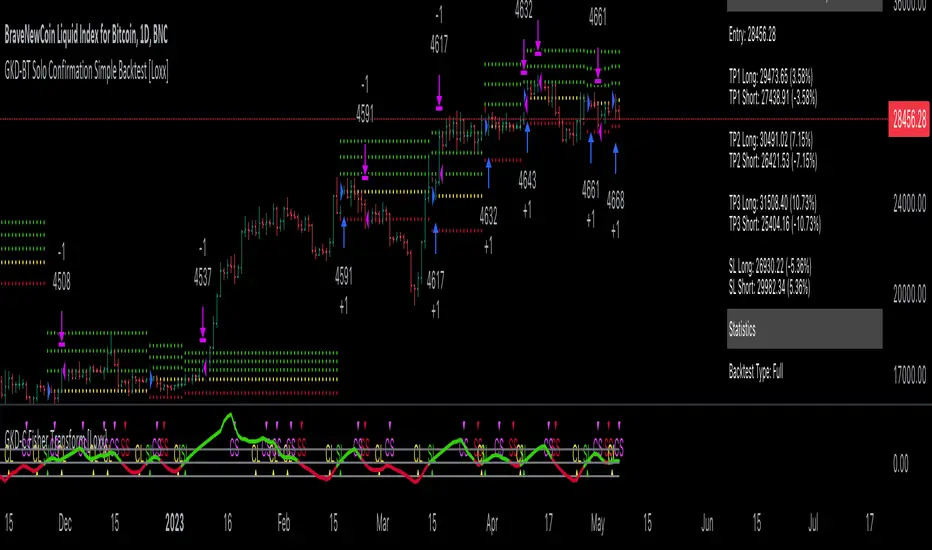
Kioseff Trading - AI-Optimized RSIAI-Optimized RSI
Introducing AI-Optimized RSI: a streamlined solution for traders of any skill level seeking to rapidly test and optimize RSI. Capable of analyzing thousands of strategies, this tool cuts through the complexity to identify the most profitable, reliable, or efficient approaches.
Paired with TradingView's native backtesting capabilities, the AI-Optimized RSI learns from historical performance data. Set up is easy for all skill levels, and it makes fine-tuning trading alerts and RSI straightforward.
Features
Purpose : Uncover optimal RSI settings and entry levels with precision. Say goodbye to random guesses and arbitrary indicator use—this tool provides clear direction based on data.
Target Performance : You set the goal, and AI-RSI seeks it out, whether it's maximizing profits, efficient trading, or achieving the highest win rate.
AI-Powered : With intelligent AI recommendations, the tool dynamically fine-tunes your RSI approach, steering you towards ideal strategy performance.
Rapid Testing : Evaluate thousands of RSI strategies.
Dual Direction : Perfect both long and short RSI strategies with equal finesse.
Deep Insights : Access detailed metrics including profit factor, PnL, win rate, trade counts, and more, all within a comprehensive strategy script.
Instant Alerts : Set alerts and trade.
Full Customization : Test and optimize all RSI settings, including cross levels, profit targets and stop losses.
Simulated Execution : Explore the impact of limit orders and other trade types through simulation.
Integrative Capability : Combine your own custom indicators or others from the TradingView community for a personalized optimization experience.
Flexible Timeframes : Set your optimization and backtesting to any date range.
Key Settings
The image above shows explanations for a list of key settings for the optimizer.
Direction : This setting controls trade direction: Long or Short.
Entry Condition : Define RSI entry: Select whether to trigger trades on RSI crossunders or crossovers.
RSI Lengths Range : Choose the range of RSI periods to test and find the best one.The AI will find the best RSI period for you.
RSI Cross Range : Set the range for RSI levels where crosses trigger trade signals. The AI will find the best level for you.
Combinations : Select how many RSI strategies to compare.
Optimization Type : Choose the goal for optimization and the AI: profit, win rate, or efficiency.
Profit Target : Set your profit target with this setting.
Stop Loss : Decide your maximum allowable loss (stop loss) per trade.
Limit Order : Specify whether to include limit orders in the strategy.
Stop Type : Choose your stop strategy: a fixed stop loss or a trailing stop.
How to: Find the best RSI for trading
It's important to remember that merely having the AI-Optimized RSI on your chart doesn't automatically provide you with the best strategy. You need to follow the AI's guidance through an iterative process to discover the optimal RSI settings and strategy.
1.Starting Your Strategy Setup
Begin by deciding your goals for each trade: your profit target and stop loss. You'll also choose how to manage your stops – whether they stay put (fixed) or move with the price (trailing), and whether you want to exit trades at a specific price (limit orders). Keep the initial settings for RSI lengths and cross ranges at their default to give the tool a broad testing field. The AI's guidance will refine these settings to pinpoint the most effective ones through a process of comprehensive testing.
The image above shows our chart prior to any optimization efforts.
Note: the settings shown above in the key settings section will be used to start our demonstration.
2. Follow AI’s suggestions
Optimization Prompt: After loading your strategy, the indicator will prompt you to change the RSI length range and RSI level range to a better performing range.
Continue changing the RSI length range and RSI level range to match the indicator's suggestions until "Best Found" is displayed!
The image above shows results after we applied the tool’s suggestions. New suggestions have appeared, and we will continue to apply them.
Continue to adjust settings as recommended by the optimizer. If no better options are found, the optimizer will suggest increasing the number of combinations. Repeat this process until the optimizer indicates that the optimal setting has been identified.
Success! With the "Best Found" notification, an optimized RSI is now active. The AI will keep refining the strategy based on ongoing performance, ensuring continuous optimization.
AI Mode
AI Mode incorporates Heuristic-Based Adaptive Learning to fine-tune trading strategies in a continuous manner. This feature consists of two main components:
Heuristic-Based Decision Making: The algorithm evaluates multiple RSI-based trading strategies using specific metrics such as Profit and Loss (PNL), Win Rate, and Most Efficient Profit. These metrics act as heuristics to assist the algorithm in identifying suitable strategies for trade execution.
Online Learning: The algorithm updates the performance evaluations of each strategy based on incoming market data. This enables the system to adapt to current market conditions.
Incorporating both heuristic-based decision-making and online learning, this feature aims to provide a framework for trading strategy optimization.
Settings
AI Mode Aggressiveness:
Description: The "AI Mode Aggressiveness" setting allows you to fine-tune the AI's trading behavior. This setting ranges from “Low” to “High”, with “High” indicating a more assertive trading approach.
Functionality: This feature filters trading strategies based on a proprietary evaluation method. A higher setting narrows down the strategies that the AI will consider, leaning towards more aggressive trading. Conversely, a lower setting allows for a more conservative approach by broadening the pool of potential strategies.
Adaptive Learning Aggressiveness:
Description: When Adaptive Learning is enabled, the "Adaptive Learning Aggressiveness" setting controls how dynamically the AI adapts to market conditions using selected performance metrics.
Functionality: This setting impacts the AI's responsiveness to shifts in strategy performance. By adjusting this setting, you can control how quickly the AI moves away from strategies that may have been historically successful but are currently underperforming, towards strategies that are showing current promise.
Optimization
Trading system optimization is immensely advantageous when executed with prudence.
Technical-oriented, mechanical trading systems work when a valid correlation is methodical to the extent that an objective, precisely-defined ruleset can consistently exploit it. If no such correlation exists, or a technical-oriented system is erroneously designed to exploit an illusory correlation (absent predictive utility), the trading system will fail.
Evaluate results practically and test parameters rigorously after discovery. Simply mining the best-performing parameters and immediately trading them is unlikely a winning strategy. Put as much effort into testing strong-performing parameters and building an accompanying system as you would any other trading strategy. Automated optimization involves curve fitting - it's the responsibility of the trader to validate a replicable sequence or correlation and the trading system that exploits it.
Paid script
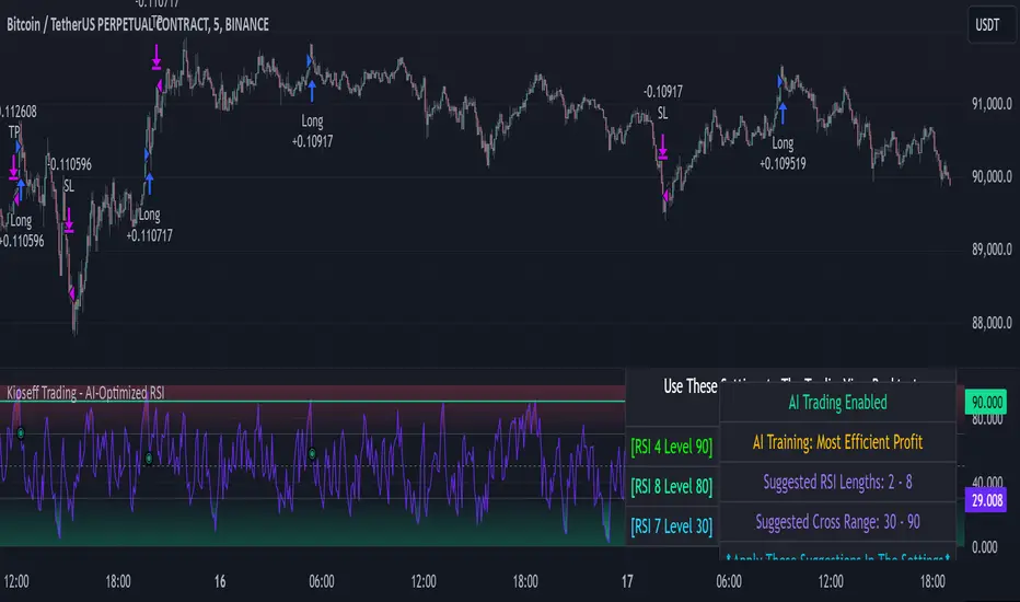
MXV trend BistroIt is so difficult for me to detect trend, maybe you.
So I need a simple trend indicator to resolve the matter
This is a trend-following indicator which condenses two simple ranges: Recommended Buy range shown with green color zone and Sell range with red color zone. To make it easy for newbies, the indicator is decorated with arrow, vertical highligted ray, buy sell signals printed on chart. When in Buy zone, do not sell. In Sell zone, do not buy
1/ When to entry and how long keeping the position?
By default, this indicator suggests that the market is trending up or down. You should make a Buy entry (up arrow) then hold long time until pivots appear, then Sell (down arrow) to exit.
2/ Which price range to entry or exit?
You should make a buy/ sell entry close to the value of recommended entry price
3/ The most appropriate time frame for this easy-to-use script is Daily
P/S
Use it for trend detect
It is very easy to use
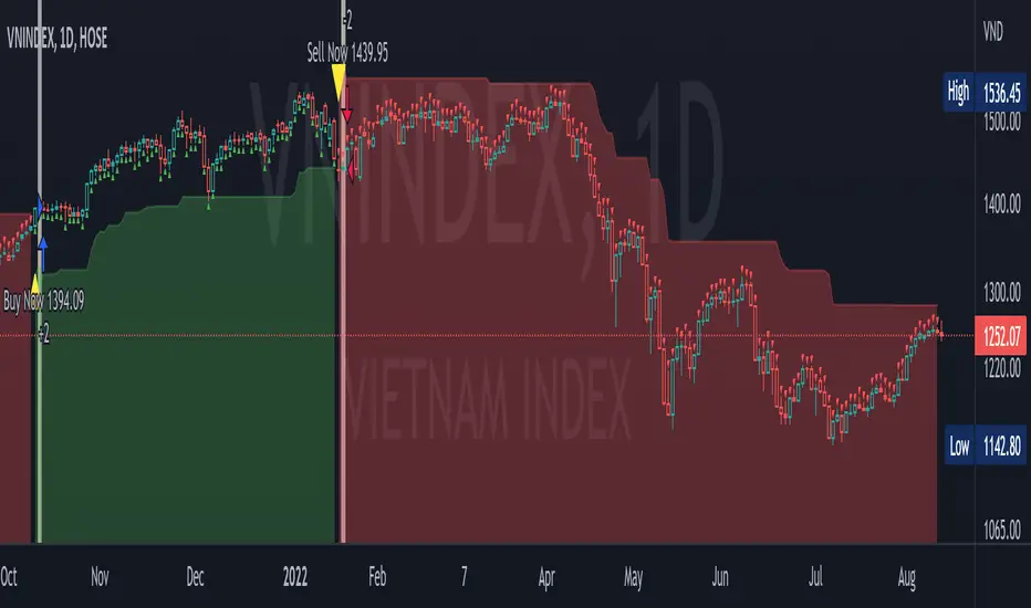
Multi-Market Swing Trader Webhook Ready [HullBuster]
Introduction
This is an all symbol swing trading strategy intended for webhook integration to live accounts. This script employs an adjustable bandwidth ping pong algorithm which can be run in long only, short only or bidirectional modes. Additionally, this script provides advanced features such as pyramiding and DCA. It has been in development for nearly three years and exposes over 90 inputs to accommodate varying risk reward ratios. Equipped with a proper configuration it is suitable for professional traders seeking quality trades from a cloud based platform. This is my most advanced Pine Script to date which combines my RangeV3 and TrendV2 scripts. Using this combination it tries to bridge the gap between range bound and trending markets. I have put a lot of time into creating a system that could transition by itself so as to require less human intervention and thus be able to withstand long periods in full automation mode.
As a Pine strategy, hypothetical performance can be easily back-tested. Allowing you to Iron out the configuration of your target instrument. Now with recent advancements from the Pine development team this same script can be connected to a webhook through the alert mechanism. The requirement of a separate study script has been completely removed. This really makes things a lot easier to get your trading system up and running. I would like to also mention that TradingView has made significant advancements to the back-end over the last year. Notably, compile times are much faster now permitting more complex algorithms to be implemented. Thank you TradingView!
I used QuantConnect as my role model and strived to produce a base script which could compete with higher end cloud based platforms while being attractive to similarly experienced traders. The versatility of the Pine Language combined with the greater selection of end point execution systems provides a powerful alternative to other cloud based platforms. At the very least, with the features available today, a modular trading system for everyday use is a reality. I hope you'll agree.
This is a swing trading strategy so the behavior of this script is to buy on weakness and sell on strength. In trading parlance this is referred to as Support and Resistance Trading. Support being the point at which prices stop falling and start rising. Resistance being the point at which prices stop rising and fall. The chart real estate between these two points being defined as the range. This script seeks to implement strategies to profit from placing trades within this region. Short positions at resistance and long positions at support. Just to be clear, the range as well as trends are merely illusions as the chart only receives prices. However, this script attempts to calculate pivot points from the price stream. Rising pivots are shorts and falling pivots are longs. I refer to pivots as a vertex in this script which adds structural components to the chart formation (point, sides and a base). When trading in “Ping Pong” mode long and short positions are interleaved continuously as long as there exists a detectable vertex.
This is a non-hedging script so those of us subject to NFA FIFO Rule 2-43(b) should be generally safe to webhook into signals emitted from this script. However, as covered later in this document, there are some technical limitations to this statement. I have tested this script on various instruments for over two years and have configurations for forex, crypto and stocks. This script along with my TrendV2 script are my daily trading vehicles as a webhook into my forex and crypto accounts. This script employs various high risk features that could wipe out your account if not used judiciously. You should absolutely not use this script if you are a beginner or looking for a get-rich-quick strategy. Also please see my CFTC RULE 4.41 disclosure statement at the end of the document. Really!
Does this script repaint? The short answer is yes, it does, despite my best efforts to the contrary. EMAs are central to my strategy and TradingView calculates from the beginning of the series so there is just no getting around this. However, Pine is improving everyday and I am hopeful that this issue will be address from an architectural level at some point in the future. I have programmed my webhook to compensate for this occurrence so, in the mean time, this my recommended way to handle it (at the endpoint and before the broker).
Design
This strategy uses a ping pong algorithm of my own design. Basically, trades bounce off each other along the price stream. Trades are produced as a series of reversals. The point at which a trade reverses is a pivot calculation. A measurement is made between the recent valley to peak which results in a standard deviation value. This value is an input to implied probability calculation.Yes, the same implied probability used in sports betting. Odds are then calculated to determine the likelihood of price action continuing or retracing to the pivot. Based on where the account is at alert time, the action could be an entry, take profit or pyramid signal. In this design, trades must occur in alternating sequence. A long followed by a short then another long followed by a short and so on. In range bound price action trades appear along the outer bands of the channel in the aforementioned sequence. Shorts on the top and longs at the bottom. Generally speaking, the widths of the trading bands can be adjusted using the vertex dynamics in Section 2. There are a dozen inputs in this section used to describe the trading range. It is not a simple adjustment. If pyramids are enabled the strategy overrides the ping pong reversal pattern and begins an accumulation sequence. In this case you will see a series of same direction trades.
This script uses twelve indicators on a single time frame. The original trading algorithms are a port from a C++ program on proprietary trading platform. I’ve converted some of the statistical functions to use standard indicators available on TradingView. The setups make heavy use of the Hull Moving Average in conjunction with EMAs that form the Bill Williams Alligator as described in his book “New Trading Dimensions” Chapter 3. Lag between the Hull and the EMAs play a key role in identifying the pivot points. I really like the Hull Moving Average. I use it in all my systems, including 3 other platforms. It’s is an excellent leading indicator and a relatively light calculation.
The trend detection algorithms rely on several factors:
1. Smoothed EMAs in a Willams Alligator pattern.
2. Number of pivots encountered in a particular direction.
3. Which side debt is being incurred.
4. Settings in Section 4 and 5 (long and short)
The strategy uses these factors to determine the probability of prices continuing in the most recent direction. My TrendV2 script uses a higher time frame to determine trend direction. I can’t use that method in this script without exceeding various TradingView limitations on code size. However, the higher time frame is the best way to know which trend is worth pursuing or better to bet against.
The entire script is around 2400 lines of Pine code which pushes the limits of what can be created on this platform given the TradingView maximums for: local scopes, run-time duration and compile time. The module has been through numerous refactoring passes and makes extensive use of ternary statements. As such, It takes a full minute to compile after adding it to a chart. Please wait for the hovering dots to disappear before attempting to bring up the input dialog box. Scrolling the chart quickly may bring up an hour glass.
Regardless of the market conditions: range or trend. The behavior of the script is governed entirely by the 91 inputs. Depending on the settings, bar interval and symbol, you can configure a system to trade in small ranges producing a thousand or more trades. If you prefer wider ranges with fewer trades then the vertex detection settings in Section 2 should employ stiffer values. To make the script more of a trend follower, adjustments are available in Section 4 and 5 (long and short respectively). Overall this script is a range trader and the setups want to get in that way. It cannot be made into a full blown trend trading system. My TrendV2 is equipped for that purpose. Conversely, this script cannot be effectively deployed as a scalper either. The vertex calculation require too much data for high frequency trading. That doesn’t work well for retail customers anyway. The script is designed to function in bar intervals between 5 minutes and 4 hours. However, larger intervals require more backtest data in order to create reliable configurations. TradingView paid plans (Pro) only provide 10K bars which may not be sufficient. Please keep that in mind.
The transition from swing trader to trend follower typically happens after a stop is hit. That means that your account experiences a loss first and usually with a pyramid stack so the loss could be significant. Even then the script continues to alternate trades long and short. The difference is that the strategy tries to be more long on rising prices and more short on falling prices as opposed to simply counter trend trading. Otherwise, a continuous period of rising prices results in a distinctly short pyramid stack. This is much different than my TrendV2 script which stays long on peaks and short on valleys. Basically, the plan is to be profitable in range bound markets and just lose less when a trend comes along. How well this actually plays out will depend largely on the choices made in the sectioned input parameters.
Sections
The input dialog for this script contains 91 inputs separated into six sections.
Section 1: Global settings for the strategy including calculation model, trading direction, exit levels, pyramid and DCA settings. This is where you specify your minimum profit and stop levels. You should setup your Properties tab inputs before working on any of the sections. It’s really important to get the Base Currency right before doing any work on the strategy inputs. It is important to understand that the “Minimum Profit” and “Limit Offset” are conditional exits. To exit at a profit, the specified value must be exceeded during positive price pressure. On the other hand, the “Stop Offset” is a hard limit.
Section 2: Vertex dynamics. The script is equipped with four types of pivot point indicators. Histogram, candle, fractal and transform. Despite how the chart visuals may seem. The chart only receives prices. It’s up to the strategy to interpret patterns from the number stream. The quality of the feed and the symbol’s bar characteristics vary greatly from instrument to instrument. Each indicator uses a fundamentally different pattern recognition algorithm. Use trial and error to determine the best fit for your configuration. After selecting an indicator type, there are eight analog fields that must be configured for that particular indicator. This is the hardest part of the configuration process. The values applied to these fields determine how the range will be measured. They have a big effect on the number of trades your system will generate. To see the vertices click on the “Show Markers” check box in this section. Red markers are long positions and blue markers are short. This will give you an idea of where trades will be placed in natural order.
Section 3: Event thresholds. Price spikes are used to enter and exit trades. The magnitude which define these spikes are configured here. The rise and fall events are primarily for pyramid placement. The rise and fall limits determine the exit threshold for the conditional “Limit Offset” field found in Section 1. These fields should be adjusted one at a time. Use a zero value to disengage every one but the one you are working on. Use the fill colors found in Section 6 to get a visual on the values applied to these fields. To make it harder for pyramids to enter stiffen the Event values. This is more of a hack as the formal pyramid parameters are in Section 1.
Section 4 and 5: Long and short settings. These are mirror opposite settings with all opposing fields having the same meaning. Its really easy to introduce data mining bias into your configuration through these fields. You must combat against this tendency by trying to keep your settings as uniform as possible. Wildly different parameters for long and short means you have probably fitted the chart. There are nine analog and thirteen Boolean fields per trade direction. This section is all about how the trades themselves will be placed along the range defined in Section 2. Generally speaking, more restrictive settings will result in less trades but higher quality. Remember that this strategy will enter long on falling prices and short on rising prices. So getting in the trade too early leads to a draw-down. However, this could be what you want if pyramiding is enabled. I, personally, have found that the best configurations come from slightly skewing one side. I just accept that the other side will be sub-par.
Section 6: Chart rendering. This section contains one analog and four Boolean fields. More or less a diagnostic tool. Of particular interest is the “Symbol Debt Sequence” field. This field contains a whole number which paints regions that have sustained a run of bad trades equal or greater than specified value. It is useful when DCA is enabled. In this script Dollar Cost Averaging on new positions continues only until the symbol debt is recouped. To get a better understanding on how this works put a number in this field and activate DCA. You should notice how the trade size increases in the colored regions. The “Summary Report” checkbox displays a blue information box at the live end of the chart. It exposes several metrics which you may find useful if manually trading this strategy from audible alerts or text messages.
Pyramids
This script features a downward pyramiding strategy which increases your position size on losing trades. On purely margin trades, this feature can be used to, hypothetically, increase the profit factor of positions (not individual trades). On long only markets, such as crypto, you can use this feature to accumulate coins at depressed prices. The way it works is the stop offset, applied in the Section 1 inputs, determines the maximum risk you intend to bear. Additional trades will be placed at pivot points calculated all the way down to the stop price. The size of each add on trade is increased by a multiple of its interval. The maximum number of intervals is limited by the “Pyramiding” field in the properties tab. The rate at which pyramid positions are created can be adjusted in Section 1. To see the pyramids click on the “Mark Pyramid Levels” check box in the same section. Blue triangles are painted below trades other than the primary.
Unlike traditional Martingale strategies, the result of your trade is not dependent on the profit or loss from the last trade. The position must recover the R1 point in order to close. Alternatively, you can set a “Pyramid Bale Out Offset” in Section 1 which will terminate the trade early. However, the bale out must coincide with a pivot point and result in a profitable exit in order to actually close the trade. Should the market price exceed the stop offset set in Section 1, the full value of the position, multiplied by the accepted leverage, will be realized as a loss to the trading account. A series of such losses will certainly wipe out your account.
Pyramiding is an advanced feature intended for professional traders with well funded accounts and an appropriate mindset. The availability of this feature is not intended to endorse or promote my use of it. Use at your own risk (peril).
DCA
In addition to pyramiding this script employs DCA which enables users to experiment with loss recovery techniques. This is another advanced feature which can increase the order size on new trades in response to stopped out or winning streak trades. The script keeps track of debt incurred from losing trades. When the debt is recovered the order size returns to the base amount specified in the properties tab. The inputs for this feature are found in section 3 and include a limiter to prevent your account from depleting capital during runaway markets. The main difference between DCA and pyramids is that this implementation of DCA applies to new trades while pyramids affect open positions. DCA is a popular feature in crypto trading but can leave you with large “bags” if your not careful. In other markets, especially margin trading, you’ll need a well funded account and much experience.
To be sure pyramiding and dollar cost averaging is as close to gambling as you can get in respectable trading exchanges. However, if you are looking to compete in a spot trading contest or just want to add excitement to your trading life style those features could find a place in your strategies. Although your backtest may show spectacular gains don’t expect your live trading account to do the same. Every backtest has some measure of data mining bias. Please remember that.
Webhook Integration
The TradingView alerts dialog provides a way to connect your script to an external system which could actually execute your trade. This is a fantastic feature that enables you to separate the data feed and technical analysis from the execution and reporting systems. Using this feature it is possible to create a fully automated trading system entirely on the cloud. Of course, there is some work to get it all going in a reliable fashion. To that end this script has several things going for it. First off, it is a strategy type script. That means that the strategy place holders such as {{strategy.position_size}} can be embedded in the alert message text. There are more than 10 variables which can write internal script values into the message for delivery to the specified endpoint. Additionally, my scripts output the current win streak and debt loss counts in the {{strategy.order.alert_message}} field. Depending on the condition, this script will output other useful values in the JSON “comment” field of the alert message. Here is an excerpt of the fields I use in my webhook signal:
"broker_id": "kraken",
"account_id": "XXX XXXX XXXX XXXX",
"symbol_id": "XMRUSD",
"action": "{{strategy.order.action}}",
"strategy": "{{strategy.order.id}}",
"lots": "{{strategy.order.contracts}}",
"price": "{{strategy.order.price}}",
"comment": "{{strategy.order.alert_message}}",
"timestamp": "{{time}}"
Though TradingView does a great job in dispatching your alert this feature does come with a few idiosyncrasies. Namely, a single transaction call in your script may cause multiple transmissions to the endpoint. If you are using placeholders each message describes part of the transaction sequence. A good example is closing a pyramid stack. Although the script makes a single strategy.close() call, the endpoint actually receives a close message for each pyramid trade. The broker, on the other hand, only requires a single close. The incongruity of this situation is exacerbated by the possibility of messages being received out of sequence. Depending on the type of order designated in the message, a close or a reversal. This could have a disastrous effect on your live account. This broker simulator has no idea what is actually going on at your real account. Its just doing the job of running the simulation and sending out the computed results. If your TradingView simulation falls out of alignment with the actual trading account lots of really bad things could happen. Like your script thinks your are currently long but the account is actually short. Reversals from this point forward will always be wrong with no one the wiser. Human intervention will be required to restore congruence. But how does anyone find out this is occurring? In closed systems engineering this is known as entropy. In practice your webhook logic should be robust enough to detect these conditions. Be generous with the placeholder usage and give the webhook code plenty of information to compare states. Both issuer and receiver. Don’t blindly commit incoming signals without verifying system integrity.
Operation
This is a swing trading strategy so the fundamental behavior of this script is to buy on weakness and sell on strength. As such trade orders are placed in a counter direction to price pressure. What you will see on the chart is a short position on peaks and a long position on valleys. This is slightly misleading since a range as well as a trend are best recognized, in hindsight, after the patterns occur on the chart. In the middle of a trade, one never knows how deep valleys will drop or how high peaks will rise. For certain, long trades will continue to trigger as the market prices fall and short trades on rising prices. This means that the maximum efficiency of this strategy is achieved in choppy markets where the price doesn’t extend very far from its adjacent pivot point. Conversely, this strategy will be the least efficient when market conditions exhibit long continuous single direction price pressure. Especially, when measured in weeks. Translation, the trend is not your friend with this strategy. Internally, the script attempts to recognize prolonged price pressure and changes tactics accordingly. However, at best, the goal is to weather the trend until the range bound market returns. At worst, trend detection fails and pyramid trades continue to be placed until the limit specified in the Properties tab is reached. In all likelihood this could trigger a margin call and if it hits the stop it could wipe out your account.
This script has been in beta test four times since inception. During all that time no one has been successful in creating a configuration from scratch. Most people give up after an hour or so. To be perfectly honest, the configuration process is a bear. I know that but there is no way, currently, to create libraries in Pine. There is also no way specify input parameters other than the flattened out 2-D inputs dialog. And the publish rules clearly state that script variations addressing markets or symbols (suites) are not permitted. I suppose the problem is systemic to be-all-end-all solutions like my script is trying to be. I needed a cloud strategy for all the symbols that I trade and since Pine does not support library modules, include files or inter process communication this script and its unruly inputs are my weapon of choice in the war against the market forces. It takes me about six hours to configure a new symbol. Also not all the symbols I configure are equally successful. I should mention that I have a facsimile of this strategy written in another platform which allows me to run a backtest on 10 years of historical data. The results provide me a sanity check on the inputs I select on this platform.
My personal configurations use a 10 minute bar interval on forex instruments and 15 minutes on crypto. I try to align my TradingView scripts to employ standard intervals available from the broker so that I can backtest longer durations than those available on TradingView. For example, Bitcoin at 15 minute bars is downloadable from several sources. I really like the 10 minute bar. It provides lots of detectable patterns and is easy to store many years in an SQL database.
The following steps provide a very brief set of instructions that will get you started but will most certainly not produce the best backtest. A trading system that you are willing to risk your hard earned capital will require a well crafted configuration that involves time, expertise and clearly defined goals. As previously mentioned, I have several example configurations that I use for my own trading that I can share with you if you like. To get hands on experience in setting up your own symbol from scratch please follow the steps below.
Step 1. Setup the Base currency and order size in the properties tab.
Step 2. Select the calculation presets in the Instrument Type field.
Step 3. Select “No Trade” in the Trading Mode field
Step 4. Select the Histogram indicator from Section 2. You will be experimenting with different ones so it doesn’t matter which one you try first.
Step 5. Turn on Show Markers in Section 2.
Step 6. Go to the chart and checkout where the markers show up. Blue is up and red is down. Long trades show up along the red markers and short trades on the blue.
Step 7. Make adjustments to “Base To Vertex” and “Vertex To Base” net change and ROC in Section 2. Use these fields to move the markers to where you want trades to be.
Step 8. Try a different indicator from Section 2 and repeat Step 7 until you find the best match for this instrument on this interval. This step is complete when the Vertex settings and indicator combination produce the most favorable results.
Step 9. Go to Section 4 and enable “Apply Red Base To Base Margin”.
Step 10. Go to Section 5 and enable “Apply Blue Base To Base Margin”.
Step 11. Go to Section 2 and adjust “Minimum Base To Base Blue” and “Minimum Base To Base Red”. Observe the chart and note where the markers move relative to each other. Markers further apart will produce less trades but will reduce cutoffs in “Ping Pong” mode.
Step 12. Turn off Show Markers in Section 2.
Step 13. Put in your Minimum Profit and Stop Loss in the first section. This is in pips or currency basis points (chart right side scale). Percentage is not currently supported. Note that the profit is taken as a conditional exit on a market order not a fixed limit. The actual profit taken will almost always be greater than the amount specified. The stop loss, on the other hand, is indeed a hard number which is executed by the TradingView broker simulator when the threshold is breached.
Step 14. Return to step 3 and select a Trading Mode (Long, Short, BiDir, Ping Pong). If you are planning to trade bidirectionally its best to configure long first then short. Combine them with “BiDir” or “Ping Pong” after setting up both sides of the trade individually. The difference between “BiDir” and “Ping Pong” is that “Ping Pong” uses position reversal and can cut off opposing trades less than the specified minimum profit. As a result “Ping Pong” mode produces the greatest number of trades.
Step 15. Take a look at the chart. Trades should be showing along the markers plotted earlier.
Step 16. Make adjustments to the Vertex fields in Section 2 until the TradingView performance report is showing a profit. This includes the “Minimum Base To Base” fields. If a profit cannot be achieved move on to Step 17.
Step 17. Improve the backtest profitability by adjusting the “Entry Net Change” and “Entry ROC” in Section 4 and 5.
Step 18. Enable the “Mandatory Snap” checkbox in Section 4 and 5 and adjust the “Snap Candle Delta” and “Snap Fractal Delta” in Section 2. This should reduce some chop producing unprofitable reversals.
Step 19. Increase the distance between opposing trades by adding an “Interleave Delta” in Sections 4 and 5. This is a floating point value which starts at 0.01 and typically does not exceed 2.0.
Step 20. Increase the distance between opposing trades even further by adding a “Decay Minimum Span” in Sections 4 and 5. This is an absolute value specified in the symbol’s quote currency (right side scale of the chart). This value is similar to the minimum profit and stop loss fields in Section 1.
Step 21. The “Buy Composite Strength” input works in tandem with “Long Decay Minimum Span” in Section 4. Try enabling and see if it improves the performance. This field is only relevant when there is a value in “Long Decay Minimum Span”.
Step 22. The “Sell Composite Weakness” input works in tandem with “Short Decay Minimum Span” in Section 5. Try enabling and see if it improves the performance. This field is only relevant when there is a value in “Short Decay Minimum Span”.
Step 23. Improve the backtest profitability by adjusting the “Adherence Delta” in Section 4 and 5. This field requires the “Adhere to Rising Trend” checkbox to be enabled.
Step 24. At this point your strategy should be more or less working. Experiment with the remaining check boxes in Section 4 and 5. Keep the ones which seem to improve the performance.
Step 25. Examine the chart and see that trades are being placed in accordance with your desired trading goals. This is an important step. If your desired model requires multiple trades per day then you should be seeing hundreds of trades on the chart. Alternatively, you may be looking to trade fewer steep peaks and deep valleys in which case you should see trades at major turning points. Don’t simply settle for what the backtest serves you. Work your configuration until the system aligns with your desired model. Try changing indicators and even intervals if you cannot reach your simulation goals. Generally speaking, the histogram and Candle indicators produce the most trades. The Fractal indicator captures the tallest peaks and valleys. The Transform indicator is the most reliable but doesn’t well work on all instruments.
Example Settings
To reproduce the performance shown on the chart please use the following configuration:
1. Select XBTUSD Kraken as the chart symbol.
2. On the properties tab set the Order Size to: 0.01 Bitcoin
3. On the properties tab set the Pyramiding to: 10
4. In Section 1: Select “Forex” for the Instrument Type
5. In Section 1: Select “Ping Pong” for the Trading Mode
6. In Section 1: Input 1200 for the Minimum Profit
7. In Section 1: Input 15000 for the Stop Offset
8. In Section 1: Input 1200 for the Pyramid Minimum Span
9. In Section 1: Check mark the Ultra Wide Pyramids
10. In Section 2: Check mark the Use Transform Indicator
So to be clear, I used a base position size of one - one hundredth of a Bitcoin and allow the script to add up to 10 downward pyramids. The example back-test did hit eight downward pyramids. That means the account would have to be able to withstand a base position size (0.01) times 28. The resulting position size is 0.28 of a Bitcoin. If the price of Bitcoin is 35K then the draw down amount (not including broker fees) would be $9800 dollars. Since I have a premium subscription my backtest chart includes 20K historical bars. That's roughly six months of data. As of today, pro accounts only get 10K bars so the performance cannot be exactly matched with such a difference in historical data. Please keep that in mind.
There are, of course, various ways to reduce the risk incurred from accumulating pyramids. You can increase the “Pyramid Minimum Span” input found in Section 2 which increases the space between each pyramid trade. Also you can set a “Pyramid Bale Out Offset” in the same input section. This lets you out of the trade faster on position recovery. For example: Set a value of 8000 into this input and the number of trades increase to 178 from 157. Since the positions didn’t go full term, more trades were created at less profit each. The total brute force approach would be to simply limit the number of pyramids in the Properties tab.
It should be noted that since this is crypto, accumulating on the long side may be what you want. If you are not trading on margin and thus outright buying coins on the Kraken exchange you likely are interested in increasing your Bitcoin position at depressed prices. This is a popular feature on some of the other crypto trading packages like CryptoHopper and Profit Trailer. Click on Enable TV Long Only Rule in Section 1. This switches the signal emitter to long only. However, you may still see short trades on the chart. They are treated as a close instead of a reversal.
Feel free to PM me with any questions related to this script. Thank you and happy trading!
CFTC RULE 4.41
These results are based on simulated or hypothetical performance results that have certain inherent limitations. Unlike the results shown in an actual performance record, these results do not represent actual trading. Also, because these trades have not actually been executed, these results may have under-or over-compensated for the impact, if any, of certain market factors, such as lack of liquidity. Simulated or hypothetical trading programs in general are also subject to the fact that they are designed with the benefit of hindsight. No representation is being made that any account will or is likely to achieve profits or losses similar to these being shown.
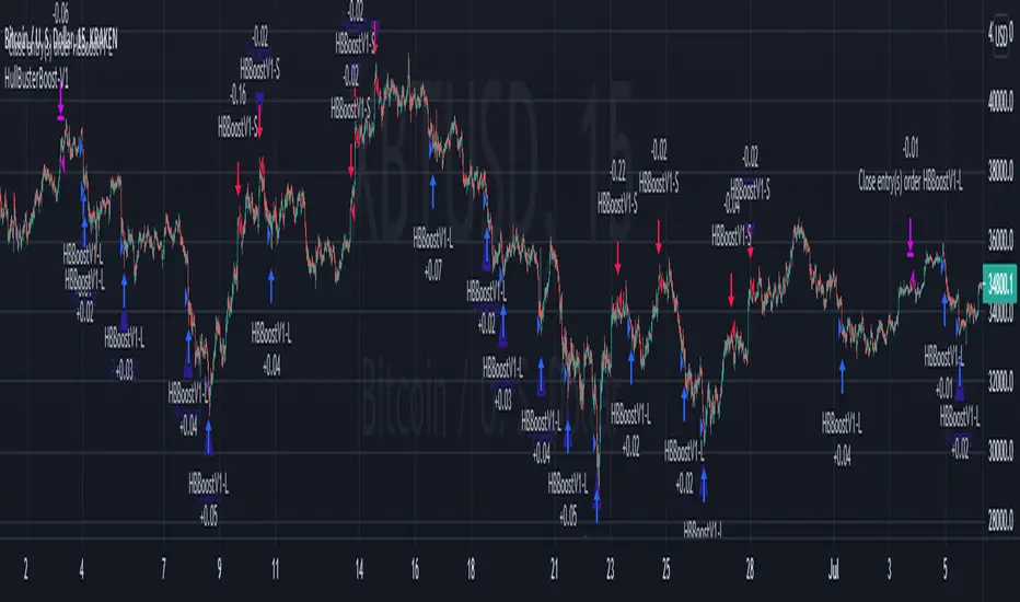
Liquid Pulse Liquid Pulse by Dskyz (DAFE) Trading Systems
Liquid Pulse is a trading algo built by Dskyz (DAFE) Trading Systems for futures markets like NQ1!, designed to snag high-probability trades with tight risk control. it fuses a confluence system—VWAP, MACD, ADX, volume, and liquidity sweeps—with a trade scoring setup, daily limits, and VIX pauses to dodge wild volatility. visuals include simple signals, VWAP bands, and a dashboard with stats.
Core Components for Liquid Pulse
Volume Sensitivity (volumeSensitivity) controls how much volume spikes matter for entries. options: 'Low', 'Medium', 'High' default: 'High' (catches small spikes, good for active markets) tweak it: 'Low' for calm markets, 'High' for chaos.
MACD Speed (macdSpeed) sets the MACD’s pace for momentum. options: 'Fast', 'Medium', 'Slow' default: 'Medium' (solid balance) tweak it: 'Fast' for scalping, 'Slow' for swings.
Daily Trade Limit (dailyTradeLimit) caps trades per day to keep risk in check. range: 1 to 30 default: 20 tweak it: 5-10 for safety, 20-30 for action.
Number of Contracts (numContracts) sets position size. range: 1 to 20 default: 4 tweak it: up for big accounts, down for small.
VIX Pause Level (vixPauseLevel) stops trading if VIX gets too hot. range: 10 to 80 default: 39.0 tweak it: 30 to avoid volatility, 50 to ride it.
Min Confluence Conditions (minConditions) sets how many signals must align. range: 1 to 5 default: 2 tweak it: 3-4 for strict, 1-2 for more trades.
Min Trade Score (Longs/Shorts) (minTradeScoreLongs/minTradeScoreShorts) filters trade quality. longs range: 0 to 100 default: 73 shorts range: 0 to 100 default: 75 tweak it: 80-90 for quality, 60-70 for volume.
Liquidity Sweep Strength (sweepStrength) gauges breakouts. range: 0.1 to 1.0 default: 0.5 tweak it: 0.7-1.0 for strong moves, 0.3-0.5 for small.
ADX Trend Threshold (adxTrendThreshold) confirms trends. range: 10 to 100 default: 41 tweak it: 40-50 for trends, 30-35 for weak ones.
ADX Chop Threshold (adxChopThreshold) avoids chop. range: 5 to 50 default: 20 tweak it: 15-20 to dodge chop, 25-30 to loosen.
VWAP Timeframe (vwapTimeframe) sets VWAP period. options: '15', '30', '60', '240', 'D' default: '60' (1-hour) tweak it: 60 for day, 240 for swing, D for long.
Take Profit Ticks (Longs/Shorts) (takeProfitTicksLongs/takeProfitTicksShorts) sets profit targets. longs range: 5 to 100 default: 25.0 shorts range: 5 to 100 default: 20.0 tweak it: 30-50 for trends, 10-20 for chop.
Max Profit Ticks (maxProfitTicks) caps max gain. range: 10 to 200 default: 60.0 tweak it: 80-100 for big moves, 40-60 for tight.
Min Profit Ticks to Trail (minProfitTicksTrail) triggers trailing. range: 1 to 50 default: 7.0 tweak it: 10-15 for big gains, 5-7 for quick locks.
Trailing Stop Ticks (trailTicks) sets trail distance. range: 1 to 50 default: 5.0 tweak it: 8-10 for room, 3-5 for fast locks.
Trailing Offset Ticks (trailOffsetTicks) sets trail offset. range: 1 to 20 default: 2.0 tweak it: 1-2 for tight, 5-10 for loose.
ATR Period (atrPeriod) measures volatility. range: 5 to 50 default: 9 tweak it: 14-20 for smooth, 5-9 for reactive.
Hardcoded Settings volLookback: 30 ('Low'), 20 ('Medium'), 11 ('High') volThreshold: 1.5 ('Low'), 1.8 ('Medium'), 2 ('High') swingLen: 5
Execution Logic Overview trades trigger when confluence conditions align, entering long or short with set position sizes. exits use dynamic take-profits, trailing stops after a profit threshold, hard stops via ATR, and a time stop after 100 bars.
Features Multi-Signal Confluence: needs VWAP, MACD, volume, sweeps, and ADX to line up.
Risk Control: ATR-based stops (capped 15 ticks), take-profits (scaled by volatility), and trails.
Market Filters: VIX pause, ADX trend/chop checks, volatility gates. Dashboard: shows scores, VIX, ADX, P/L, win %, streak.
Visuals Simple signals (green up triangles for longs, red down for shorts) and VWAP bands with glow. info table (bottom right) with MACD momentum. dashboard (top right) with stats.
Chart and Backtest:
NQ1! futures, 5-minute chart. works best in trending, volatile conditions. tweak inputs for other markets—test thoroughly.
Backtesting: NQ1! Frame: Jan 19, 2025, 09:00 — May 02, 2025, 16:00 Slippage: 3 Commission: $4.60
Fee Typical Range (per side, per contract)
CME Exchange $1.14 – $1.20
Clearing $0.10 – $0.30
NFA Regulatory $0.02
Firm/Broker Commis. $0.25 – $0.80 (retail prop)
TOTAL $1.60 – $2.30 per side
Round Turn: (enter+exit) = $3.20 – $4.60 per contract
Disclaimer this is for education only. past results don’t predict future wins. trading’s risky—only use money you can lose. backtest and validate before going live. (expect moderators to nitpick some random chart symbol rule—i’ll fix and repost if they pull it.)
About the Author Dskyz (DAFE) Trading Systems crafts killer trading algos. Liquid Pulse is pure research and grit, built for smart, bold trading. Use it with discipline. Use it with clarity. Trade smarter. I’ll keep dropping badass strategies ‘til i build a brand or someone signs me up.
2025 Created by Dskyz, powered by DAFE Trading Systems. Trade smart, trade bold.
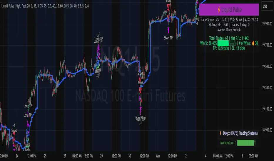
FreedX Grid Backtest█ FreedX Grid Backtest is an open-source tool that offers accurate GRID calculations for GRID trading strategies. This advanced tool allows users to backtest GRID trading parameters with precision, accurately reflecting exchange functionalities. We are committed to enhancing trading strategies through precise backtesting solutions and address the issue of unreliable backtesting practices observed on GRID trading strategies. FreedX Grid Backtest is designed for optimal calculation speed and plotting efficiency, ensuring users to achieve fastest calculations during their analysis.
█ GRID TRADING STRATEGY SETTINGS
The core of the FreedX Grid Backtest tool lies in its ability to simulate grid trading strategies. Grid trading involves placing orders at regular intervals within a predefined price range, creating a grid of orders that capitalize on market volatility.
Features:
⚙️ Backtest Range:
→ Purpose: Allows users to specify the backtesting range of GRID strategy. Closes all positions at the end of this range.
→ How to Use: Drag the dates to fit the desired backtesting range.
⚙️ Investment & Compounding:
→ Purpose: Allows users to specify the total investment amount and select between fixed and compound investment strategies. Compounding adjusts trade quantities based on performance, enhancing the grid strategy's adaptability to market changes.
→ How to Use: Set the desired investment amount and choose between "Fixed" or "Compound" for the investment method.
⚙️ Leverage & Grid Levels:
→ Purpose: Leverage amplifies the investment amount, increasing potential returns (and risks). Users can define the number of grid levels, which determines how the investment is distributed across the grid.
→ How to Use: Input the desired leverage and number of grids. The tool automatically calculates the distribution of funds across each grid level.
⚙️ Distribution Type & Mode:
→ Purpose: Users can select the distribution type (Arithmetic or Geometric) to set how grid levels are determined. The mode (Neutral, Long, Short) dictates the direction of trades within the grid.
→ How to Use: Choose the distribution type and mode based on the desired trading strategy and market outlook.
⚙️ Enable LONG/SHORT Grids exclusively:
█ MANUAL LEVELS AND STOP TRIGGERS
Beyond automated settings, the tool offers manual adjustments for traders seeking finer control over their grid strategies.
Features:
⚙️ Manual Level Adjustment:
→ Purpose: Enables traders to manually set the top, reference, and bottom levels of the grid, offering precision control over the trading range.
→ How to Use: Activate manual levels and adjust the top, reference, and bottom levels as needed to define the grid's scope.
⚙️ Stop Triggers:
→ Purpose: Provides an option to set upper and lower price limits, acting as stop triggers to close or terminate trades. This feature safeguards investments against significant market movements outside the anticipated range.
→ How to Use: Enable stop triggers and specify the upper and lower limits. The tool will automatically manage positions based on these parameters.
---
This guide gives you a quick and clear overview of the FreedX Grid Backtest tool, explaining how you can use this cutting-edge tool to improve your trading strategies.

Master Supertrend Strategy [Trendoscope]Here is the strategy version of the indicator - Master Supertrend
Options and variations are same throughout.
🎲 Variations
Following variations are provided in the form of settings.
🎯 Range Type
Instead of ATR, different types of ranges can be used for stop calculation. Here is the complete list used in the script.
Plus/Minus Range* - Calculates plus range and minus range for each candle and uses them for different sides of stop calculation
Ladder ATR - Based on the existing concept of Ladder ATR defined in Supertrend-Ladder-ATR
True Range - True range derived from standard function ta.tr
Standard Deviation - Standard deviation of close prices
🎯 Applied Calculation
In standard ATR, rma of TR is used for calculations. But, the application calculation provides option to users to use different mechanisms. It can be a type of moving average or few other types of calculations.
Available values are
sma
ema
hma
rma
wma
high
median
🎯 Other options
Few other options provided are
Use Close Price - If selected stops are calculated based on the close price instead of high/low prices
Wait for Close If selected, change of supertrend direction is calculated based on close price instead of high/low prices
Diminishing Stop Distance - When selected, stop distance for the trend direction can only reduce and cannot increase. This option is useful for keeping the tight stops on strong trends.
🎯 Plus Minus Range*
One of the range type used is Plus/Minus Range. What it means and how are these ranges calculated? Let's have a look.
Plus Range is an upward movement of a candle from its last price or open price whichever is lower.
Minus Range is a downward movement of a candle from its last price or open price whichever is higher.
This divides True Range into two separate range for positive and negative side.
Note : Effectiveness on daily charts are quire visible. However, if you want to use it for lower timeframes, please play around with settings before settling on suitable configuration.

TSI.LTA | Base BTC 1DTSI.LTA | Base BTC 1D is a closed‑source trend‑following strategy designed for BTC on the 1D timeframe .
It focuses on participating in the main directional moves of the market while avoiding as much short‑term noise as possible.
📊 The script:
Uses a combination of moving‑average–based filters and volatility bands to define the active trend.
Applies optional volume filters to avoid low‑participation or exhausted moves.
Includes risk‑management controls (Stop Loss, Take Profit, Trailing Stop) that work on a per‑trade basis.
All entries and exits are confirmed at bar close and the script does not repaint .
This makes it suitable for backtesting, alerts and external automation.
█ 💡 CONCEPTS
This strategy is built around a few simple ideas:
1 — Trend first.
Positions are only taken when a group of smoothed trend filters agree on direction.
The goal is to ride larger swings, not to scalp each fluctuation.
2 — Volatility awareness.
Standard‑deviation–based bands help avoid entries in abnormal spikes or during very compressed ranges.
3 — Participation filter.
Optional volume‑based conditions (VWMA, OBV slope, MFI, volume Z‑score) try to ensure that entries occur when the market shows enough activity, not during dead phases.
4 — Risk defined in advance.
Stop‑loss and trailing‑stop inputs are expressed as percentages relative to entry price, so users can align them with their own risk tolerance.
The logic is purposely conservative: it is expected to stay flat during parts of the market where the trend is unclear or participation is weak.
█ ⚙️ FEATURES & INPUTS
This section follows approximately the order of the script’s inputs, so users can read here and then match what they see in the “Inputs” tab.
1 — 📐 Trend filters
These inputs control how the strategy detects the underlying trend:
DEMA / Gaussian / SMMA lengths
Control how fast or slow the trend reacts to price changes.
Shorter lengths → more responsive, more trades, more noise.
Longer lengths → slower reaction, fewer trades, more filtering.
Volatility Bands (SD length & multipliers)
Standard‑deviation bands around the smoothed price series.
They are used to avoid entries during extreme moves or very narrow ranges where a breakout is not yet confirmed.
In practice, these settings let the user choose between a more “aggressive” trend follower (shorter lengths, smaller bands) or a more “patient” one.
2 — 📊 Volume filters (optional)
These filters are meant to restrict trades to periods where the market shows meaningful participation:
VWMA filter
Requires price to be aligned with a Volume‑Weighted Moving Average, which de‑emphasizes moves on very low volume.
OBV slope filter
Uses the slope of On‑Balance Volume to check that net volume flow supports the direction of the trade.
MFI band filter
Uses the Money Flow Index to avoid taking new entries in zones that often correspond to exhaustion (extreme values defined by the user).
Volume Z‑Score
Compares current volume to its recent history. Trades can be restricted when volume is unusually low or out of character for that period.
When any of these filters are turned off, the strategy relies only on price‑based trend and volatility logic.
When they are on, trades are more selective and may be fewer.
3 — 🛡️ Risk management
These inputs define how individual trades are managed once entered.
They do not change the trend logic itself:
Stop Loss (%)
A percentage move against the entry price that will close the position.
Typical values on BTC 1D remain in the single‑digit range so that no single trade risks an unrealistic portion of equity.
Take Profit (%)
An optional fixed target that closes the trade when price has moved a chosen percentage in favor.
This can be disabled if the user prefers to let the trend filters perform the exit.
Trailing Stop (%)
A stop that follows the most favorable price reached since entry.
When the “use lower timeframe peak” option is enabled, peaks can be detected on a lower timeframe for more granular trailing, while decisions still occur at the close of the 1D bar.
Fixed SL/TP Price and Activation Date
Allow defining absolute price levels and a date from which they start applying.
This is useful when the user wants structural protection around known price zones.
The combination of these controls determines how deep a pullback the user is willing to tolerate and how much profit they are prepared to give back in order to stay in trends.
4 — 🚫 Filter failure & cooldown
To avoid over‑trading in difficult environments, the script can:
Automatically exit when filters remain unfavorable for a configurable number of bars.
Enter a cooldown period, during which no new trades are taken, even if some conditions improve.
These mechanisms are intended to protect capital during choppy or low‑quality phases rather than force constant exposure.
█ 📚 HOW TO USE
A suggested process for using this strategy as a study tool:
1 — Start on BTC 1D.
Apply the script to BTCUSD or BTC/USDT on the 1D timeframe, with default inputs.
2 — Open the Strategy Tester.
Choose a time window (for example a full halving cycle, a crash + recovery period, or just the most recent bull leg).
3 — Compare with Buy & Hold.
For the same window, look at:
Net profit of the strategy vs Buy & Hold.
Max drawdown of the strategy vs Buy & Hold.
The goal is not to hit a particular number, but to see whether, in that window, the strategy manages to:
Provide a smoother equity curve (lower drawdown),
While still performing at least as well as, or better than, simply holding the asset.
4 — Experiment with risk inputs.
Vary Stop Loss, Trailing Stop and the volume filters.
After each change, re‑check the same two questions above. This should make clear how each input affects the trade‑off between participation and risk.
5 — Forward‑test.
Before using any configuration with real capital, let it run for a while in paper‑trading or demo conditions.
█ 🚧 LIMITATIONS
The strategy is built and tuned primarily for BTC on 1D.
It can be used on other symbols and timeframes, but behavior may differ and requires new testing.
In very tight ranges or during event‑driven gaps, trend logic may enter later than discretionary trading would. This is expected for a conservative trend‑following approach.
Results from historical backtests depend on data quality, broker settings, fees and slippage configured in the Strategy Tester.
█ 📝 NOTES
Signals are generated on bar close.
The script is closed‑source, but the description explains the main ideas so users and moderators can understand what it does and how to use it.
The HUD on the chart is meant as a compact summary of the same statistics available in the Strategy Tester; it simply makes comparisons quicker.
█ ⚠️ DISCLAIMER
This strategy is provided for educational and research purposes only .
It is not financial advice and does not recommend any specific trades, assets, position sizes, or risk levels.
Users are fully responsible for:
Choosing their own risk parameters (Stop Loss, Take Profit, Trailing Stop, position sizing, etc.).
Testing the script on the markets and timeframes they intend to trade.
Verifying that any configuration is appropriate for their capital, risk tolerance and jurisdiction.
Past performance in backtests or examples does not guarantee future results.
Always test carefully before considering any live deployment.

Reversal Point Dynamics - Machine Learning⇋ Reversal Point Dynamics - Machine Learning
RPD Machine Learning: Self-Adaptive Multi-Armed Bandit Trading System
RPD Machine Learning is an advanced algorithmic trading system that implements genuine machine learning through contextual multi-armed bandits, reinforcement learning, and online adaptation. Unlike traditional indicators that use fixed rules, RPD learns from every trade outcome , automatically discovers which strategies work in current market conditions, and continuously adapts without manual intervention .
Core Innovation: The system deploys six distinct trading policies (ranging from aggressive trend-following to conservative range-bound strategies) and uses LinUCB contextual bandit algorithms with Random Fourier Features to learn which policy performs best in each market regime. After the initial learning phase (50-100 trades), the system achieves autonomous adaptation , automatically shifting between policies as market conditions evolve.
Target Users: Quantitative traders, algorithmic trading developers, systematic traders, and data-driven investors who want a system that adapts over time . Suitable for stocks, futures, forex, and cryptocurrency on any liquid instrument with >100k daily volume.
The Problem This System Solves
Traditional Technical Analysis Limitations
Most trading systems suffer from three fundamental challenges :
Fixed Parameters: Static settings (like "buy when RSI < 30") work well in backtests but may struggle when markets change character. What worked in low-volatility environments may not work in high-volatility regimes.
Strategy Degradation: Manual optimization (curve-fitting) produces systems that perform well on historical data but may underperform in live trading. The system never adapts to new market conditions.
Cognitive Overload: Running multiple strategies simultaneously forces traders to manually decide which one to trust. This leads to hesitation, late entries, and inconsistent execution.
How RPD Machine Learning Addresses These Challenges
Automated Strategy Selection: Instead of requiring you to choose between trend-following and mean-reversion strategies, RPD runs all six policies simultaneously and uses machine learning to automatically select the best one for current conditions. The decision happens algorithmically, removing human hesitation.
Continuous Learning: After every trade, the system updates its understanding of which policies are working. If the market shifts from trending to ranging, RPD automatically detects this through changing performance patterns and adjusts selection accordingly.
Context-Aware Decisions: Unlike simple voting systems that treat all conditions equally, RPD analyzes market context (ADX regime, entropy levels, volatility state, volume patterns, time of day, historical performance) and learns which combinations of context features correlate with policy success.
Machine Learning Architecture: What Makes This "Real" ML
Component 1: Contextual Multi-Armed Bandits (LinUCB)
What Is a Multi-Armed Bandit Problem?
Imagine facing six slot machines, each with unknown payout rates. The exploration-exploitation dilemma asks: Should you keep pulling the machine that's worked well (exploitation) or try others that might be better (exploration)? RPD solves this for trading policies.
Academic Foundation:
RPD implements Linear Upper Confidence Bound (LinUCB) from the research paper "A Contextual-Bandit Approach to Personalized News Article Recommendation" (Li et al., 2010, WWW Conference). This algorithm is used in content recommendation and ad placement systems.
How It Works:
Each policy (AggressiveTrend, ConservativeRange, VolatilityBreakout, etc.) is treated as an "arm." The system maintains:
Reward History: Tracks wins/losses for each policy
Contextual Features: Current market state (8-10 features including ADX, entropy, volatility, volume)
Uncertainty Estimates: Confidence in each policy's performance
UCB Formula: predicted_reward + α × uncertainty
The system selects the policy with highest UCB score , balancing proven performance (predicted_reward) with potential for discovery (uncertainty bonus). Initially, all policies have high uncertainty, so the system explores broadly. After 50-100 trades, uncertainty decreases, and the system focuses on known-performing policies.
Why This Matters:
Traditional systems pick strategies based on historical backtests or user preference. RPD learns from actual outcomes in your specific market, on your timeframe, with your execution characteristics.
Component 2: Random Fourier Features (RFF)
The Non-Linearity Challenge:
Market relationships are often non-linear. High ADX may indicate favorable conditions when volatility is normal, but unfavorable when volatility spikes. Simple linear models struggle to capture these interactions.
Academic Foundation:
RPD implements Random Fourier Features from "Random Features for Large-Scale Kernel Machines" (Rahimi & Recht, 2007, NIPS). This technique approximates kernel methods (like Support Vector Machines) while maintaining computational efficiency for real-time trading.
How It Works:
The system transforms base features (ADX, entropy, volatility, etc.) into a higher-dimensional space using random projections and cosine transformations:
Input: 8 base features
Projection: Through random Gaussian weights
Transformation: cos(W×features + b)
Output: 16 RFF dimensions
This allows the bandit to learn non-linear relationships between market context and policy success. For example: "AggressiveTrend performs well when ADX >25 AND entropy <0.6 AND hour >9" becomes naturally encoded in the RFF space.
Why This Matters:
Without RFF, the system could only learn "this policy has X% historical performance." With RFF, it learns "this policy performs differently in these specific contexts" - enabling more nuanced selection.
Component 3: Reinforcement Learning Stack
Beyond bandits, RPD implements a complete RL framework :
Q-Learning: Value-based RL that learns state-action values. Maps 54 discrete market states (trend×volatility×RSI×volume combinations) to 5 actions (4 policies + no-trade). Updates via Bellman equation after each trade. Converges toward optimal policy after 100-200 trades.
TD(λ) with Eligibility Traces: Extension of Q-Learning that propagates credit backwards through time . When a trade produces an outcome, TD(λ) updates not just the final state-action but all states visited during the trade, weighted by eligibility decay (λ=0.90). This accelerates learning from multi-bar trades.
Policy Gradient (REINFORCE): Learns a stochastic policy directly from 12 continuous market features without discretization. Uses gradient ascent to increase probability of actions that led to positive outcomes. Includes baseline (average reward) for variance reduction.
Meta-Learning: The system learns how to learn by adapting its own learning rates based on feature stability and correlation with outcomes. If a feature (like volume ratio) consistently correlates with success, its learning rate increases. If unstable, rate decreases.
Why This Matters:
Q-Learning provides fast discrete decisions. Policy Gradient handles continuous features. TD(λ) accelerates learning. Meta-learning optimizes the optimization. Together, they create a robust, multi-approach learning system that adapts more quickly than any single algorithm.
Component 4: Policy Momentum Tracking (v2 Feature)
The Recency Challenge:
Standard bandits treat all historical data equally. If a policy performed well historically but struggles in current conditions due to regime shift, the system may be slow to adapt because historical success outweighs recent underperformance.
RPD's Solution:
Each policy maintains a ring buffer of the last 10 outcomes. The system calculates:
Momentum: recent_win_rate - global_win_rate (range: -1 to +1)
Confidence: consistency of recent results (1 - variance)
Policies with positive momentum (recent outperformance) get an exploration bonus. Policies with negative momentum and high confidence (consistent recent underperformance) receive a selection penalty.
Effect: When markets shift, the system detects the shift more quickly through momentum tracking, enabling faster adaptation than standard bandits.
Signal Generation: The Core Algorithm
Multi-Timeframe Fractal Detection
RPD identifies reversal points using three complementary methods :
1. Quantum State Analysis:
Divides price range into discrete states (default: 6 levels)
Peak signals require price in top states (≥ state 5)
Valley signals require price in bottom states (≤ state 1)
Prevents mid-range signals that may struggle in strong trends
2. Fractal Geometry:
Identifies swing highs/lows using configurable fractal strength
Confirms local extremum with neighboring bars
Validates reversal only if price crosses prior extreme
3. Multi-Timeframe Confirmation:
Analyzes higher timeframe (4× default) for alignment
MTF confirmation adds probability bonus
Designed to reduce false signals while preserving valid setups
Probability Scoring System
Each signal receives a dynamic probability score (40-99%) based on:
Base Components:
Trend Strength: EMA(velocity) / ATR × 30 points
Entropy Quality: (1 - entropy) × 10 points
Starting baseline: 40 points
Enhancement Bonuses:
Divergence Detection: +20 points (price/momentum divergence)
RSI Extremes: +8 points (RSI >65 for peaks, <40 for valleys)
Volume Confirmation: +5 points (volume >1.2× average)
Adaptive Momentum: +10 points (strong directional velocity)
MTF Alignment: +12 points (higher timeframe confirms)
Range Factor: (high-low)/ATR × 3 - 1.5 points (volatility adjustment)
Regime Bonus: +8 points (trending ADX >25 with directional agreement)
Penalties:
High Entropy: -5 points (entropy >0.85, chaotic price action)
Consolidation Regime: -10 points (ADX <20, no directional conviction)
Final Score: Clamped to 40-99% range, classified as ELITE (>85%), STRONG (75-85%), GOOD (65-75%), or FAIR (<65%)
Entropy-Based Quality Filter
What Is Entropy?
Entropy measures randomness in price changes . Low entropy indicates orderly, directional moves. High entropy indicates chaotic, unpredictable conditions.
Calculation:
Count up/down price changes over adaptive period
Calculate probability: p = ups / total_changes
Shannon entropy: -p×log(p) - (1-p)×log(1-p)
Normalized to 0-1 range
Application:
Entropy <0.5: Highly ordered (ELITE signals possible)
Entropy 0.5-0.75: Mixed (GOOD signals)
Entropy >0.85: Chaotic (signals blocked or heavily penalized)
Why This Matters:
Prevents trading during choppy, news-driven conditions where technical patterns may be less reliable. Automatically raises quality bar when market is unpredictable.
Regime Detection & Market Microstructure - ADX-Based Regime Classification
RPD uses Wilder's Average Directional Index to classify markets:
Bull Trend: ADX >25, +DI > -DI (directional conviction bullish)
Bear Trend: ADX >25, +DI < -DI (directional conviction bearish)
Consolidation: ADX <20 (no directional conviction)
Transitional: ADX 20-25 (forming direction, ambiguous)
Filter Logic:
Blocks all signals during Transitional regime (avoids trading during uncertain conditions)
Blocks Consolidation signals unless ADX ≥ Min Trend Strength
Adds probability bonus during strong trends (ADX >30)
Effect: Designed to reduce signal frequency while focusing on higher-quality setups.
Divergence Detection
Bearish Divergence:
Price makes higher high
Velocity (price momentum) makes lower high
Indicates weakening upward pressure → SHORT signal quality boost
Bullish Divergence:
Price makes lower low
Velocity makes higher low
Indicates weakening downward pressure → LONG signal quality boost
Bonus: Adds probability points and additional acceleration factor. Divergence signals have historically shown higher success rates in testing.
Hierarchical Policy System - The Six Trading Policies
1. AggressiveTrend (Policy 0):
Probability Threshold: 60% (trades more frequently)
Entropy Threshold: 0.70 (tolerates moderate chaos)
Stop Multiplier: 2.5× ATR (wider stops for trends)
Target Multiplier: 5.0R (larger targets)
Entry Mode: Pyramid (scales into winners)
Best For: Strong trending markets, breakouts, momentum continuation
2. ConservativeRange (Policy 1):
Probability Threshold: 75% (more selective)
Entropy Threshold: 0.60 (requires order)
Stop Multiplier: 1.8× ATR (tighter stops)
Target Multiplier: 3.0R (modest targets)
Entry Mode: Single (one-shot entries)
Best For: Range-bound markets, low volatility, mean reversion
3. VolatilityBreakout (Policy 2):
Probability Threshold: 65% (moderate)
Entropy Threshold: 0.80 (accepts high entropy)
Stop Multiplier: 3.0× ATR (wider stops)
Target Multiplier: 6.0R (larger targets)
Entry Mode: Tiered (splits entry)
Best For: Compression breakouts, post-consolidation moves, gap opens
4. EntropyScalp (Policy 3):
Probability Threshold: 80% (very selective)
Entropy Threshold: 0.40 (requires extreme order)
Stop Multiplier: 1.5× ATR (tightest stops)
Target Multiplier: 2.5R (quick targets)
Entry Mode: Single
Best For: Low-volatility grinding moves, tight ranges, highly predictable patterns
5. DivergenceHunter (Policy 4):
Probability Threshold: 70% (quality-focused)
Entropy Threshold: 0.65 (balanced)
Stop Multiplier: 2.2× ATR (moderate stops)
Target Multiplier: 4.5R (balanced targets)
Entry Mode: Tiered
Best For: Divergence-confirmed reversals, exhaustion moves, trend climax
6. AdaptiveBlend (Policy 5):
Probability Threshold: 68% (balanced)
Entropy Threshold: 0.75 (balanced)
Stop Multiplier: 2.0× ATR (standard)
Target Multiplier: 4.0R (standard)
Entry Mode: Single
Best For: Mixed conditions, general trading, fallback when no clear regime
Policy Clustering (Advanced/Extreme Modes)
Policies are grouped into three clusters based on regime affinity:
Cluster 1 (Trending): AggressiveTrend, DivergenceHunter
High regime affinity (0.8): Performs well when ADX >25
Moderate vol affinity (0.6): Works in various volatility
Cluster 2 (Ranging): ConservativeRange, AdaptiveBlend
Low regime affinity (0.3): Better suited for ADX <20
Low vol affinity (0.4): Optimized for calm markets
Cluster 3 (Breakout): VolatilityBreakout
Moderate regime affinity (0.6): Works in multiple regimes
High vol affinity (0.9): Requires high volatility for optimal characteristics
Hierarchical Selection Process:
Calculate cluster scores based on current regime and volatility
Select best-matching cluster
Run UCB selection within chosen cluster
Apply momentum boost/penalty
This two-stage process reduces learning time - instead of choosing among 6 policies from scratch, system first narrows to 1-2 policies per cluster, then optimizes within cluster.
Risk Management & Position Sizing
Dynamic Kelly Criterion Sizing (Optional)
Traditional Fixed Sizing Challenge:
Using the same position size for all signal probabilities may be suboptimal. Higher-probability signals could justify larger positions, lower-probability signals smaller positions.
Kelly Formula:
f = (p × b - q) / b
Where:
p = win probability (from signal score)
q = loss probability (1 - p)
b = win/loss ratio (average_win / average_loss)
f = fraction of capital to risk
RPD Implementation:
Uses Fractional Kelly (1/4 Kelly default) for safety. Full Kelly is theoretically optimal but can recommend large position sizes. Fractional Kelly reduces volatility while maintaining adaptive sizing benefits.
Enhancements:
Probability Bonus: Normalize(prob, 65, 95) × 0.5 multiplier
Divergence Bonus: Additional sizing on divergence signals
Regime Bonus: Additional sizing during strong trends (ADX >30)
Momentum Adjustment: Hot policies receive sizing boost, cold policies receive reduction
Safety Rails:
Minimum: 1 contract (floor)
Maximum: User-defined cap (default 10 contracts)
Portfolio Heat: Max total risk across all positions (default 4% equity)
Multi-Mode Stop Loss System
ATR Mode (Default):
Stop = entry ± (ATR × base_mult × policy_mult)
Consistent risk sizing
Ignores market structure
Best for: Futures, forex, algorithmic trading
Structural Mode:
Finds swing low (long) or high (short) over last 20 bars
Identifies fractal pivots within lookback
Places stop below/above structure + buffer (0.1× ATR)
Best for: Stocks, instruments that respect structure
Hybrid Mode (Intelligent):
Attempts structural stop first
Falls back to ATR if:
Structural level is invalid (beyond entry)
Structural stop >2× ATR away (too wide)
Best for: Mixed instruments, adaptability
Dynamic Adjustments:
Breakeven: Move stop to entry + 1 tick after 1.0R profit
Trailing: Trail stop 0.8R behind price after 1.5R profit
Timeout: Force close after 30 bars (optional)
Tiered Entry System
Challenge: Equal sizing on all signals may not optimize capital allocation relative to signal quality.
Solution:
Tier 1 (40% of size): Enters immediately on all signals
Tier 2 (60% of size): Enters only if probability ≥ Tier 2 trigger (default 75%)
Example:
Calculated optimal size: 10 contracts
Signal probability: 72%
Tier 2 trigger: 75%
Result: Enter 4 contracts only (Tier 1)
Same signal at 80% probability
Result: Enter 10 contracts (4 Tier 1 + 6 Tier 2)
Effect: Automatically scales size to signal quality, optimizing capital allocation.
Performance Optimization & Learning Curve
Warmup Phase (First 50 Trades)
Purpose: Ensure all policies get tested before system focuses on preferred strategies.
Modifications During Warmup:
Probability thresholds reduced 20% (65% becomes 52%)
Entropy thresholds increased 20% (more permissive)
Exploration rate stays high (30%)
Confidence width (α) doubled (more exploration)
Why This Matters:
Without warmup, system might commit to early-performing policy without testing alternatives. Warmup forces thorough exploration before focusing on best-performing strategies.
Curriculum Learning
Phase 1 (Trades 1-50): Exploration
Warmup active
All policies tested
High exploration (30%)
Learning fundamental patterns
Phase 2 (Trades 50-100): Refinement
Warmup ended, thresholds normalize
Exploration decaying (30% → 15%)
Policy preferences emerging
Meta-learning optimizing
Phase 3 (Trades 100-200): Specialization
Exploration low (15% → 8%)
Clear policy preferences established
Momentum tracking fully active
System focusing on learned patterns
Phase 4 (Trades 200+): Maturity
Exploration minimal (8% → 5%)
Regime-policy relationships learned
Auto-adaptation to market shifts
Stable performance expected
Convergence Indicators
System is learning well when:
Policy switch rate decreasing over time (initially ~50%, should drop to <20%)
Exploration rate decaying smoothly (30% → 5%)
One or two policies emerge with >50% selection frequency
Performance metrics stabilizing over time
Consistent behavior in similar market conditions
System may need adjustment when:
Policy switch rate >40% after 100 trades (excessive exploration)
Exploration rate not decaying (parameter issue)
All policies showing similar selection (not differentiating)
Performance declining despite relaxed thresholds (underlying signal issue)
Highly erratic behavior after learning phase
Advanced Features
Attention Mechanism (Extreme Mode)
Challenge: Not all features are equally important. Trading hour might matter more than price-volume correlation, but standard approaches treat them equally.
Solution:
Each RFF dimension has an importance weight . After each trade:
Calculate correlation: sign(feature - 0.5) × sign(reward)
Update importance: importance += correlation × 0.01
Clamp to range
Effect: Important features get amplified in RFF transformation, less important features get suppressed. System learns which features correlate with successful outcomes.
Temporal Context (Extreme Mode)
Challenge: Current market state alone may be incomplete. Historical context (was volatility rising or falling?) provides additional information.
Solution:
Includes 3-period historical context with exponential decay (0.85):
Current features (weight 1.0)
1 bar ago (weight 0.85)
2 bars ago (weight 0.72)
Effect: Captures momentum and acceleration of market features. System learns patterns like "rising volatility with falling entropy" that may precede significant moves.
Transfer Learning via Episodic Memory
Short-Term Memory (STM):
Last 20 trades
Fast adaptation to immediate regime
High learning rate
Long-Term Memory (LTM):
Condensed historical patterns
Preserved knowledge from past regimes
Low learning rate
Transfer Mechanism:
When STM fills (20 trades), patterns consolidated into LTM . When similar regime recurs later, LTM provides faster adaptation than starting from scratch.
Practical Implementation Guide - Recommended Settings by Instrument
Futures (ES, NQ, CL):
Adaptive Period: 20-25
ML Mode: Advanced
RFF Dimensions: 16
Policies: 6
Base Risk: 1.5%
Stop Mode: ATR or Hybrid
Timeframe: 5-15 min
Forex Majors (EURUSD, GBPUSD):
Adaptive Period: 25-30
ML Mode: Advanced
RFF Dimensions: 16
Policies: 6
Base Risk: 1.0-1.5%
Stop Mode: ATR
Timeframe: 5-30 min
Cryptocurrency (BTC, ETH):
Adaptive Period: 20-25
ML Mode: Extreme (handles non-stationarity)
RFF Dimensions: 32 (captures complexity)
Policies: 6
Base Risk: 1.0% (volatility consideration)
Stop Mode: Hybrid
Timeframe: 15 min - 4 hr
Stocks (Large Cap):
Adaptive Period: 25-30
ML Mode: Advanced
RFF Dimensions: 16
Policies: 5-6
Base Risk: 1.5-2.0%
Stop Mode: Structural or Hybrid
Timeframe: 15 min - Daily
Scaling Strategy
Phase 1 (Testing - First 50 Trades):
Max Contracts: 1-2
Goal: Validate system on your instrument
Monitor: Performance stabilization, learning progress
Phase 2 (Validation - Trades 50-100):
Max Contracts: 2-3
Goal: Confirm learning convergence
Monitor: Policy stability, exploration decay
Phase 3 (Scaling - Trades 100-200):
Max Contracts: 3-5
Enable: Kelly sizing (1/4 Kelly)
Goal: Optimize capital efficiency
Monitor: Risk-adjusted returns
Phase 4 (Full Deployment - Trades 200+):
Max Contracts: 5-10
Enable: Full momentum tracking
Goal: Sustained consistent performance
Monitor: Ongoing adaptation quality
Limitations & Disclaimers
Statistical Limitations
Learning Sample Size: System requires minimum 50-100 trades for basic convergence, 200+ trades for robust learning. Early performance (first 50 trades) may not reflect mature system behavior.
Non-Stationarity Risk: Markets change over time. A system trained on one market regime may need time to adapt when conditions shift (typically 30-50 trades for adjustment).
Overfitting Possibility: With 16-32 RFF dimensions and 6 policies, system has substantial parameter space. Small sample sizes (<200 trades) increase overfitting risk. Mitigated by regularization (λ) and fractional Kelly sizing.
Technical Limitations
Computational Complexity: Extreme mode with 32 RFF dimensions, 6 policies, and full RL stack requires significant computation. May perform slowly on lower-end systems or with many other indicators loaded.
Pine Script Constraints:
No true matrix inversion (uses diagonal approximation for LinUCB)
No cryptographic RNG (uses market data as entropy)
No proper random number generation for RFF (uses deterministic pseudo-random)
These approximations reduce mathematical precision compared to academic implementations but remain functional for trading applications.
Data Requirements: Needs clean OHLCV data. Missing bars, gaps, or low liquidity (<100k daily volume) can degrade signal quality.
Forward-Looking Bias Disclaimer
Reward Calculation Uses Future Data: The RL system evaluates trades using an 8-bar forward-looking window. This means when a position enters at bar 100, the reward calculation considers price movement through bar 108.
Why This is Disclosed:
Entry signals do NOT look ahead - decisions use only data up to entry bar
Forward data used for learning only, not signal generation
In live trading, system learns identically as bars unfold in real-time
Simulates natural learning process (outcomes are only known after trades complete)
Implication: Backtested metrics reflect this 8-bar evaluation window. Live performance may vary if:
- Positions held longer than 8 bars
- Slippage/commissions differ from backtest settings
- Market microstructure changes (wider spreads, different execution quality)
Risk Warnings
No Guarantee of Profit: All trading involves substantial risk of loss. Machine learning systems can fail if market structure fundamentally changes or during unprecedented events.
Maximum Drawdown: With 1.5% base risk and 4% max total risk, expect potential drawdowns. Historical drawdowns do not predict future drawdowns. Extreme market conditions can exceed expectations.
Black Swan Events: System has not been tested under: flash crashes, trading halts, circuit breakers, major geopolitical shocks, or other extreme events. Such events can exceed stop losses and cause significant losses.
Leverage Risk: Futures and forex involve leverage. Adverse moves combined with leverage can result in losses exceeding initial investment. Use appropriate position sizing for your risk tolerance.
System Failures: Code bugs, broker API failures, internet outages, or exchange issues can prevent proper execution. Always monitor automated systems and maintain appropriate safeguards.
Appropriate Use
This System Is:
✅ A machine learning framework for adaptive strategy selection
✅ A signal generation system with probabilistic scoring
✅ A risk management system with dynamic sizing
✅ A learning system designed to adapt over time
This System Is NOT:
❌ A price prediction system (does not forecast exact prices)
❌ A guarantee of profits (can and will experience losses)
❌ A replacement for due diligence (requires monitoring and understanding)
❌ Suitable for complete beginners (requires understanding of ML concepts, risk management, and trading fundamentals)
Recommended Use:
Paper trade for 100 signals before risking capital
Start with minimal position sizing (1-2 contracts) regardless of calculated size
Monitor learning progress via dashboard
Scale gradually over several months only after consistent results
Combine with fundamental analysis and broader market context
Set account-level risk limits (e.g., maximum drawdown threshold)
Never risk more than you can afford to lose
What Makes This System Different
RPD implements academically-derived machine learning algorithms rather than simple mathematical calculations or optimization:
✅ LinUCB Contextual Bandits - Algorithm from WWW 2010 conference (Li et al.)
✅ Random Fourier Features - Kernel approximation from NIPS 2007 (Rahimi & Recht)
✅ Q-Learning, TD(λ), REINFORCE - Standard RL algorithms from Sutton & Barto textbook
✅ Meta-Learning - Learning rate adaptation based on feature correlation
✅ Online Learning - Real-time updates from streaming data
✅ Hierarchical Policies - Two-stage selection with clustering
✅ Momentum Tracking - Recent performance analysis for faster adaptation
✅ Attention Mechanism - Feature importance weighting
✅ Transfer Learning - Episodic memory consolidation
Key Differentiators:
Actually learns from trade outcomes (not just parameter optimization)
Updates model parameters in real-time (true online learning)
Adapts to changing market regimes (not static rules)
Improves over time through reinforcement learning
Implements published ML algorithms with proper citations
Conclusion
RPD Machine Learning represents a different approach from traditional technical analysis to adaptive, self-learning systems . Instead of manually optimizing parameters (which can overfit to historical data), RPD learns behavior patterns from actual trading outcomes in your specific market.
The combination of contextual bandits, reinforcement learning, random fourier features, hierarchical policy selection, and momentum tracking creates a multi-algorithm learning system designed to handle non-stationary markets better than static approaches.
After the initial learning phase (50-100 trades), the system achieves autonomous adaptation - automatically discovering which strategies work in current conditions and shifting allocation without human intervention. This represents an approach where systems adapt over time rather than remaining static.
Use responsibly. Paper trade extensively. Scale gradually. Understand that past performance does not guarantee future results and all trading involves risk of loss.
Taking you to school. — Dskyz, Trade with insight. Trade with anticipation.

Kaito Box with RSI Div(Dynamic Adjustment + MA + Long)The script implements a dynamic trading strategy that combines box range detection, RSI divergence signals, and moving average trend analysis. It is designed for use on OKX Signal Bots and includes features for dynamic position scaling and partial position closing. Below is a summary of its key functionalities:
Key Features:
Box Range Detection:
The script identifies price ranges using the highest high and lowest low of a configurable boxLength period.
These levels are plotted on the chart to visualize the price range.
RSI Divergence Detection:
The script calculates RSI using a configurable rsiLength.
Detects bullish divergence when price makes a lower low, but RSI makes a higher low.
Detects bearish divergence when price makes a higher high, but RSI makes a lower high.
Includes separate left and right lookback periods (leftLookback, rightLookback) for precise local extrema detection.
Customizable Moving Averages:
Supports multiple types of Moving Averages (SMA, EMA, SMMA, WMA, VWMA).
Calculates and plots MA20, MA50, MA100, and MA200 on a user-defined timeframe (custom_timeframe).
Identifies uptrends and downtrends based on the alignment of the moving averages and price levels.
Dynamic Position Scaling:
Implements dynamic position sizing for long entries and partial position closing for exits.
The percentage of position size added or closed is based on the difference between the current price and the average position price (avgPrice), with configurable minimum thresholds (minEnterPercent, minExitPercent).
Signal Integration for OKX Bots:
Sends buy/sell signals to OKX Signal Bots using the configured signalToken.
Supports market or limit orders with configurable price offsets and investment types.
Trend-Based Signal Filtering:
Only triggers long signals during downtrends and short signals during uptrends, ensuring trades align with the overall market context.
Visual Annotations:
Plots bullish and bearish divergence signals on the chart.
Displays labels showing dynamic position size adjustments and current average price during trades.
How It Works:
Long Signals:
Triggered when the price breaches the lower box range, and a bullish RSI divergence is detected.
Additional filtering ensures long trades are executed only during downtrend conditions.
Dynamically adjusts the position size based on the price difference from the average entry price.
Short Signals:
Triggered when the price breaches the upper box range, and a bearish RSI divergence is detected.
Additional filtering ensures short trades are executed only during uptrend conditions.
Dynamically closes portions of the position based on price movement relative to the average entry price.
Alerts:
Generates actionable alerts formatted for OKX bots, including order type, signal token, and dynamically calculated position sizes.
Use Case:
This strategy is well-suited for automated trading on platforms like OKX, where it can:
Exploit price ranges and RSI divergences for precise entries and exits.
Dynamically manage position sizes to optimize risk-reward.
Adapt to different market conditions using configurable parameters like moving averages, divergence lookbacks, and trend filters.
This script provides a robust foundation for traders looking to automate their strategies while maintaining flexibility and control over their trading logic.

Flux Charts - PAT Automation💎 GENERAL OVERVIEW
The PAT Automation is a powerful and versatile tool designed to help traders rigorously test their trading strategies against historical market data. With an array of advanced settings, traders can fine-tune their strategies, assess performance, and identify key improvements before deploying in live trading environments. This backtester offers a wide range of configurable settings, explained within this write-up.
Features of the PAT Automation:
Step By Step : Configure your strategy step by step, which will allow you to have OR & AND logic in your strategies.
Highly Configurable : Offers multiple parameters for fine-tuning trade entry and exit conditions.
Multi-Timeframe Analysis : Allows traders to analyze multiple timeframes simultaneously for enhanced accuracy.
Provides advanced stop-loss, take-profit, and break-even settings.
Incorporates volume-based conditions, liquidity grabs , order blocks , market structures and fair value gaps for refined strategy execution.
🚩 UNIQUENESS
The PAT Automation stands out from conventional backtesting tools due to its unparalleled flexibility, precision, and advanced trading logic integration. Key factors that make it unique include:
✅ Comprehensive Strategy Customization – Unlike traditional backtesters that offer basic entry and exit conditions, PAT Automation provides a highly detailed parameter set, allowing traders to fine-tune their strategies with precision.
✅ Multi-Timeframe Price Action Features – This is the first-ever tool that allows traders to backtest price action with multi-timeframe features such as Fair Value Gaps (FVGs), Inversion Fair Value Gaps (IFVGs), Order Blocks & Breaker Blocks.
✅ Customizable Take-Profit Conditions – Offers various methods to set take-profit exits, including using core features from price action, and fixed exits like ATR, % change or price change, enabling traders to tailor their exit strategies to specific market behaviors.
✅ Customizable Stop-Loss Conditions – Provides several ways to set up stop losses, including using concepts from price action and trailing stops or fixed exits like ATR, % change or price change, allowing for dynamic risk management tailored to individual strategies.
✅ Integration of External Indicators – Allows the inclusion of other indicators or data sources from TradingView for creating strategy conditions, enabling traders to enhance their strategies with additional insights and data points.
By integrating these advanced features, PAT Automation ensures that traders can rigorously test and optimize their strategies with great accuracy and efficiency.
📌 HOW DOES IT WORK?
The first setting you will want to set it the pyramiding setting. This setting controls the number of simultaneous trades in the same direction allowed in the strategy. For example, if you set it to 1, only one trade can be active in any time, and the second trade will not be entered unless the first one is exited. If it is set to 2, the script will handle both of them at the same time. Note that you should enter the same value to this pyramiding setting, and the pyramiding setting in the "Properties" tab of the script for this to work.
For deep backtesting, you can set "Max Distance To Last Bar" to "Unlimited". If you encounter any memory issues, try decreasing this setting to a lower value.
You can enable and set a backtesting window that will limit the entries to between the start date & end date.
Then, you can enter your desired settings to Price Action features like FVGs, IFVGs, Order Blocks, Breaker Blocks, Liquidity Grabs, Market Structures, EQH & EQL and Volume Imbalances. You can also enable and set up to 3 timeframes, which you can use later on when customizing your strategies enter / exit conditions.
Entry Conditions
From the "Long Conditions" or the "Short Conditions" groups, you can set your position entry conditions. For settings like "initial capital" or "order size", you can open the "Properties" tab, where these are handled.
The PAT Automation can use the following conditions for entry conditions :
1. Order Block (OB)
Detection: Triggered when an Order Block forms or is detected
Retest: Triggered when price retests an Order Block. A retest is confirmed when a candle enters an Order Block and closes outside of it.
Retracement: Triggered when price touches an Order Block
Break: Triggered when an Order Block is invalidated by candle close or wick, depending on the user's input.
2. Breaker Block (BB)
Detection: Triggered when a Breaker Block forms or is detected
Retest: Triggered when price retests a Breaker Block. A retest is confirmed when a candle enters a Breaker Block and closes outside of it.
Retracement: Triggered when price touches a Breaker Block
Break: Triggered when a Breaker Block is invalidated by candle close or wick, depending on the user's input.
3. Fair Value Gap (FVG)
Detection: Triggered when an FVG forms or is detected
Retest: Triggered when price retests an FVG. A retest is confirmed when a candle enters an FVG and closes outside of it.
Retracement: Triggered when price touches an FVG
Break: Triggered when an FVG is invalidated by candle close or wick, depending on the user's input.
4. Inversion Fair Value Gap (IFVG)
Detection: Triggered when an IFVG forms or is detected
Retest: Triggered when price retests an IFVG. A retest is confirmed when a candle enters an IFVG and closes outside of it.
Retracement: Triggered when price touches an IFVG
Break: Triggered when an IFVG is invalidated by candle close or wick, depending on the user's input.
5. Break of Structure (BOS)
Detection: Triggered when a BOS forms or is detected
6. Change of Character (CHoCH)
Detection: Triggered when a CHoCH forms or is detected
7. Change of Character Plus (CHoCH+)
Detection: Triggered when a CHoCH+ forms or is detected
8. Volume Imbalance (VI)
Detection: Triggered when a Volume Imbalance forms or is detected
9. Equal High (EQH)
Detection: Triggered when an EQH is detected
10. Equal Low (EQL)
Detection: Triggered when an EQL is detected
11. Buyside Liquidity Grab
Detection: Triggered when a liquidity grab occurs at Buyside Liquidity (BSL).
12. Sellside Liquidity Grab
Detection: Triggered when a liquidity grab occurs at Sellside Liquidity (SSL).
🕒 TIMEFRAME CONDITIONS
The PAT Automation supports Multi-Timeframe (MTF) features, just like the Price Action Toolkit. When setting an entry condition, you can also choose the timeframe.
To set up MTF conditions, navigate to the 'Timeframes' section in the settings, select your desired timeframes, and enable them. You can choose up to three timeframes.
Once you've selected your timeframes, you can use them in your strategy. When setting long and short entry / exit conditions, you can choose from Timeframe 1, Timeframe 2, or Timeframe 3.
External Conditions
Users can use external indicators on the chart to set entry conditions.
The second dropdown in the external condition settings allows you to choose a conditional operator to compare external outputs. Available options include:
Less Than or Equal To: <=
Less Than: <
Equal To: =
Greater Than: >
Greater Than or Equal To: >=
The position entry conditions work like this ;
Each side has 5 Price Action conditions and 1 Source condition. Each condition can be enabled or disabled using the checkbox on the left side.
For Price Action Conditions, you can set a direction: "Any", "Bullish" or "Bearish".
Then a Price Action Feature, like "FVG" or "Order Block".
The last part of our constructed condition is the alert type, which you can select between "Detection", "Retest", "Retracement" or "Break".
Now you should have a constructed condition, which should look like "Bullish Order Block Retest".
You can select which timeframe should this condition work on from Timeframe 1, 2 or 3. If you select "Any Timeframe", the condition will work for all timeframes.
Lastly select the step of this condition from 1 to 6.
The Source Condition
The last condition on each side is a source condition that is different from the others. Using this condition, you can create your own logic using other indicators' outputs on your chart. For example, suppose that you have an EMA indicator in your chart. You can have the source condition to something like "EMA > high".
The Step System
Each condition has a step number, and conditions are in topological order based on them.
The conditions are executed step by step. This means the condition with step 2 cannot be executed before the condition with step 1 is executed.
Conditions with the same step numbers have "OR" logic. This means that if you have 2 conditions with step 3, the condition with step 4 can trigger after only one of the step 3 conditions is executed.
➕ OTHER ENTRY FEATURES
The PAT Automation allows traders to choose when to execute trades and when not to execute trades.
1. Only Take Trades
This setting lets users specify the time period when their strategy can open or execute trades.
2. Don't Take Trades
This setting lets users specify time periods when their strategy can't open or execute trades.
↩️ EXIT CONDITIONS
1. Exit on Opposite Signal
When enabled, a long position will close when short entry conditions are met, and a short position will close when long entry conditions are met.
2. Exit on Session End
When enabled, positions will be closed at the end of the trading session.
📈 TAKE PROFIT CONDITIONS
There are several methods available for setting take profit exits and conditions.
1. Entry Condition TP
Users can use entry conditions as triggers for take-profit exits. This setting can be found under the long and short exit conditions.
2. Fixed TP
Users can set a fixed TP for exits. This setting can be found under the long and short exit conditions. Users can choose between the following:
Price: This method triggers a TP exit when price reaches a specified level. For example, if you set the Price TP to 10 and buy NASDAQ:TSLA at $190, the trade will automatically exit when the price reaches $200 ($190 + $10).
Ticks: This method triggers a TP exit when price moves a specified number of ticks.
Percentage (%): This method triggers a TP exit when price moves a specified percentage.
ATR: This method triggers a TP exit based on a specified multiple of the Average True Range (ATR).
📉 STOP LOSS CONDITIONS
There are several methods available for setting stop-loss exits and conditions.
1. Entry Condition SL
Users can use entry conditions as triggers for stop-loss exits. This setting can be found under the long and short exit conditions.
2. Fixed SL
Users can set a fixed SL for exits. This setting can be found under the long and short exit conditions. Users can choose between the following:
Price: This method triggers a SL exit when price reaches a specified level. For example, if you set the Price SL to 10 and buy NASDAQ:TSLA at $200, the trade will automatically exit when the price reaches $190 ($200 - $10).
Ticks: This method triggers a SL exit when price moves a specified number of ticks.
Percentage (%): This method triggers a SL exit when price moves a specified percentage.
ATR: This method triggers a SL exit based on a specified multiple of the Average True Range (ATR).
3. Trailing Stop
An explanation & example for the trailing stop feature is present on the write-up within the next section.
Exit conditions have the same logic of constructing conditions like the entry ones. You can construct a Take-Profit Condition & a Stop-Loss Condition. Note that the Take-Profit condition will only work if the position is in profit, regardless of if it's triggered or not. The same applies for the Stop-Loss condition, meaning that it will only work if the position is in loss.
You can also set a Fixed TP & Fixed SL based on the price movement after the position is entered. You have options like "Price", "Ticks", "%", or "Average True Range". For example, you can set a Fixed TP like "5%", and the position will be entered once it moves 5% up in a long position.
Trailing Stop
For the Fixed SL, you also have a "Trailing" stop option, which you can set it's activation level as well. The Trailing stop activation level and it's value are expressed in ticks. Check this scenerio for an example :
We have a ticker with a tick value of $1. Our Trailing Stop is set to 10 ticks and activation level is set to 30 ticks.
We buy 1 contract when the price is $100.
When the price becomes $110, we are in $10 (10 ticks) profit and the trailing stop is now activated.
The current price our stop's on is $110 - $30 (30 ticks), which is the level of $80.
The trailing stop will only move if the price moves up the highest high the price has been after we entered the position.
Let's suppose that price moves up $40 right after our trailing stop is activated. The price will now be $150, and our trailing stop will sit on $150 - $30 (30 ticks) = $120.
If the price is down the $120 level, our stop loss will be triggered.
There is also a "Hard SL" option designed for a backup stop-loss when trailing stops are enabled. You can enable & set this option and if the price goes down before our trailing stop even activates, the position will be exited.
You can also move stop-loss to the break-even (entry price of the position) after a certain profit is achieved using the last setting of the exit conditions. Note that for this to work, you will need to have a Fixed SL set-up.
➕ OTHER EXIT FEATURES
1. Move Stop Loss to Breakeven
This setting allows the strategy to automatically move the SL to Breakeven (BE) when the position is in profit by a certain amount. Users can choose between the following:
Price: This method moves the SL to BE when price reaches a specified level.
Ticks: This method moves the SL to BE when price moves a specified number of ticks.
Percentage (%): This method moves the SL to BE when price moves a specified percentage.
ATR: This method moves the SL to BE when price moves a specified multiple of the Average True Range (ATR).
Example Entry Scenario
To give an example , check this scenario; out conditions are :
LONG CONDITIONS
Bullish Order Block Detection, Step 1
Bullish CHoCH Detection, Step 2
Bullish Volume Imbalance Detection, Step 2
Bullish IFVG Retest, Step 3
First, the strategy needs to detect a Bullish Order Block in order to start working.
After it's detected, now it's looking for either a CHoCH, or a Volume Imbalance to proceed to the next step, the reason for this is that they both have the same step number.
After one of them is detected, the strategy will consistently check all IFVGs for a retest. If the retest occurs, a long position will be entered.
⏰ ALERTS
This indicator uses TradingView's strategy alert system. All entries and exits will be sent as an alert if configured. It's possible to further customize these alerts to your liking. For more information check TradingView's strategy alert customization page: www.tradingview.com
⚙️ SETTINGS
1. Backtesting Settings
Pyramiding: Controls the number of simultaneous trades allowed in the strategy. This setting must have the same value that is entered on the script's properties tab on the settings pane.
Max Distance to Last Bar: Determines the depth of historical data used to prevent memory overload.
Enable Custom Backtesting Period: Restricts backtesting to a specific date range.
Start & End Time Configuration: Define precise start and end dates for historical analysis.
2. Fair Value Gaps Settings
Zone Invalidation: Select between "Wick" and "Close" invalidation.
Filtering: Choose between "Average Range" and "Volume Threshold".
FVG Sensitivity: Ranges from Extreme to Low to detect FVGs with varying strictness.
Allow Gaps: Enables analysis on tickers that have different open-close price gaps.
3. Inversion Fair Value Gaps Settings
Zone Invalidation: Choose between "Wick" and "Close".
4. Order Block Settings
Swing Length: Adjusts the minimum number of bars required for OB formation.
Zone Invalidation Method: Select between "Wick" and "Close".
5. Breaker Block Settings
Zone Invalidation: Set invalidation method as "Wick" or "Close".
6. Liquidity Grabs Settings
Pivot Length: Adjusts the number of bars used to detect liquidity grabs.
Wick-Body Ratio: Defines the proportion of wick-to-body size for liquidity grab detection.
7. Multi-Timeframe Analysis
Enable Up to Three Timeframes: Select and analyze trades across multiple timeframes.
8. Market Structures
Swing Length: Defines the number of bars required for structure shifts.
Includes BOS, CHoCH, CHoCH+ Detection.
9. Equal Highs & Lows
ATR Multiplier: Defines the sensitivity of equal highs/lows detection.
10. Volume Imbalances
Gap Size Sensitivity: Ranges from "Ultra" to "Low".
Disable Overnight Gaps: Filters out volume imbalances occurring due to overnight gaps.
11. Entry Conditions for Long & Short Trades
Multiple Conditions (1-6): Configure up to six independent conditions per trade direction.
Condition Types: Options include Detection, Retest, Retracement, and Break.
Timeframe Specification: Choose between "Any Timeframe", "Timeframe 1", "Timeframe 2", or "Timeframe 3".
Trade Execution Filters: Restrict trades within specific trading sessions.
12. Exit Conditions for Long & Short Trades
Exit on Opposite Signal: Automatically exit trades upon opposite trade conditions.
Exit on Session End: Closes all positions at the end of the trading session.
Multiple Take-Profit (TP) and Stop-Loss (SL) Configurations:
TP/SL based on % move, ATR, Ticks, or Fixed Price.
Hard SL option for additional risk control.
Move SL to BE (Break Even) after a certain profit threshold.

Volume ValueWhen VelocityTitle: Volume ValueWhen Velocity Trading Strategy
▶ Introduction:
The " Volume ValueWhen Velocity " trading strategy is designed to generate long position signals based on various technical conditions, including volume thresholds, RSI (Relative Strength Index), and price action relative to the Simple Moving Average (SMA). The strategy aims to identify potential buy opportunities when specific criteria are met, helping traders capitalize on potential bullish movements.
▶ How to use and conditions
★ Important : Only on Spot Binance BINANCE:BTCUSDT
Name: Volume ValueWhen Velocity
Operating mode: Long on Spot BINANCE BINANCE:BTCUSDT
Timeframe: Only one hour
Market: Crypto
currency: Bitcoin only
Signal type: Medium or short term
Entry: All sections in the Technical Indicators and Conditions section must be saved to enter (This is explained below)
Exit: Based on loss limit and profit limit It is removed in the settings section
Backtesting:
⁃ Exchange: BINANCE BINANCE:BTCUSDT
⁃ Pair: BTCUSDT
⁃ Timeframe:1h
⁃ Fee: 0.1%
- Initial Capital: 1,000 USDT
- Position sizing: 500 usdt
-Trading Range: 2022-07-01 11:30 ___ 2023-07-21 14:30
▶ Strategy Settings and Parameters:
1. `strategy(title='Volume ValueWhen Velocity', ...`: Sets the strategy title, initial capital, default quantity type, default quantity value, commission value, and trading currency.
↬ Stop-Loss and Take-Profit Settings:
1. long_stoploss_value and long_stoploss_percentage : Define the stop-loss percentage for long positions.
2. long_takeprofit_value and long_takeprofit_percentage : Define the take-profit percentage for long positions.
↬ ValueWhen Occurrence Parameters:
1. occurrence_ValueWhen_1 and occurrence_ValueWhen_2 : Control the occurrences of value events.
2. `distance_value`: Specifies the minimum distance between occurrences of ValueWhen 1 and ValueWhen 2.
↬ RSI Settings:
1. rsi_over_sold and rsi_length : Define the oversold level and RSI length for RSI calculations.
↬ Volume Thresholds:
1. volume_threshold1 , volume_threshold2 , and volume_threshold3 : Set the volume thresholds for multiple volume conditions.
↬ ATR (Average True Range) Settings:
1. atr_small and atr_big : Specify the periods used to calculate the Average True Range.
▶ Date Range for Back-Testing:
1. start_date, end_date, start_month, end_month, start_year, and end_year : Define the date range for back-testing the strategy.
▶ Technical Indicators and Conditions:
1. rsi: Calculates the Relative Strength Index (RSI) based on the defined RSI length and the closing prices.
2. was_over_sold: Checks if the RSI was oversold in the last 10 bars.
3. getVolume and getVolume2 : Custom functions to retrieve volume data for specific bars.
4. firstCandleColor : Evaluates the color of the first candle based on different timeframes.
5. sma : Calculates the Simple Moving Average (SMA) of the closing price over 13 periods.
6. numCandles : Counts the number of candles since the close price crossed above the SMA.
7. atr1 : Checks if the ATR_small is less than ATR_big for the specified security and timeframe.
8. prevClose, prevCloseBarsAgo, and prevCloseChange : ValueWhen functions to calculate the change in the close price between specific occurrences.
9. atrval: A condition based on the ATR_value3.
▶ Buy Signal Condition:
Condition: A combination of multiple volume conditions.
buy_signal: The final buy signal condition that considers various technical conditions and their interactions.
▶ Long Strategy Execution:
1. The strategy will enter a long position (buy) when the buy_signal condition is met and within the specified date range.
2. A stop-loss and take-profit will be set for the long position to manage risk and potential profits.
▶ Conclusion:
The " Volume ValueWhen Velocity " trading strategy is designed to identify long position opportunities based on a combination of volume conditions, RSI, and price action. The strategy aims to capitalize on potential bullish movements and utilizes a stop-loss and take-profit mechanism to manage risk and optimize potential returns. Traders can use this strategy as a starting point for their own trading systems or further customize it to suit their preferences and risk appetite. It is crucial to thoroughly back-test and validate any trading strategy before deploying it in live markets.
↯ Disclaimer:
Risk Management is crucial, so adjust stop loss to your comfort level. A tight stop loss can help minimise potential losses. Use at your own risk.
How you or we can improve? Source code is open so share your ideas!
Leave a comment and smash the boost button!
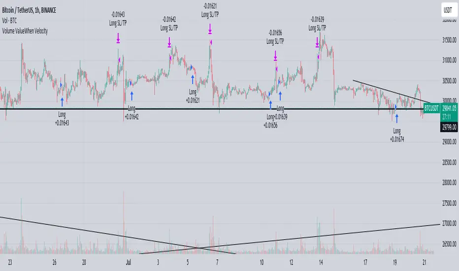
VWolf – Apex GateOverview
VWolf – Apex Gate is a trend-continuation system that blends a Pivot-weighted Supertrend (PVT ST) with an optional **Normal Supertrend** trigger, all **gated by a 200-EMA directional filter. The strategy’s risk controls are volatility-aware—**stops and targets scale by ATR**, and quantity is computed from a fixed **% risk per trade**. Clear **Backtest / Forwardtest** modes with date windows let you validate on segmented datasets before committing to live use.
Recommended Use
- **Markets:** High-liquidity instruments (indices, large-cap equities, liquid FX and major crypto pairs) where trends and pullbacks are clean.
- **Timeframes:** 15m–1h for active intraday; 4h–1D for swing. Lower timeframes may benefit from stricter EMA gating and slightly wider ATR stops.
- **Workflow:**
1. Start with **Backtest** to set baseline ATR/EMA parameters.
2. Move to **Forwardtest** to confirm generalization.
3. Consider walk-forward or multi-symbol rotation to assess robustness.
Strengths & Precautions
Strengths
- **Dual engine** (PVT ST + Normal ST) improves signal quality; the **EMA gate** screens counter-trend noise.
- **ATR-native** stops/targets standardize risk across regimes/instruments.
- **Capital-proportional sizing** preserves account geometry and smooths drawdowns.
- **Clear test segmentation** supports objective evaluation.
Precautions
- **Whipsaw risk** in tight ranges: widen ATR multipliers, enable the EMA gate, or require co-confirmation.
- **Supertrend-anchored stops** can expand in volatility spikes; ensure **% risk** remains within tolerance.
- **One-position policy** avoids stacking risk but forgoes scaling into strong trends; advanced users may prefer add-on frameworks outside this baseline.
Conclusion
VWolf – Apex Gate seeks to enter shortly after **regime flips**, demanding alignment between a **pivot-aware Supertrend** and (optionally) a **classic Supertrend**, while an **EMA gate** enforces directional discipline. With **ATR-driven** stops/targets and **fixed-fraction** sizing, the system adapts naturally to changing volatility. Use the **Backtest** window to dial ranges and the **Forwardtest** window to prove durability on unseen data. For best results, tailor ATR multipliers and the EMA gate to your instrument’s structure and your personal drawdown tolerance.

SigmaKernel - AdaptiveSigmaKernel - Adaptive Self-Optimizing Multi-Factor Trading System
SigmaKernel - Adaptive is a self-learning algorithmic trading strategy that combines four distinct analytical dimensions—momentum, market structure, volume flow, and reversal patterns—within a machine-learning-inspired framework that continuously adjusts its own parameters based on realized trading performance. Unlike traditional fixed-parameter strategies that maintain static weightings regardless of market conditions or results, this system implements a feedback loop that tracks which signal types, directional biases, and market conditions produce profitable outcomes, then mathematically adjusts component weightings, minimum score thresholds, position sizing multipliers, and trade spacing requirements to optimize future performance.
The strategy is designed for futures traders operating on prop firm accounts or live capital, incorporating realistic execution mechanics including configurable entry modes (stop breakout orders, limit pullback entries, or market-on-open), commission structures calibrated to retail futures contracts ($0.62 per contract default), one-tick slippage modeling, and professional risk controls including trailing drawdown guards, daily loss limits, and weekly profit targets. The system features universal futures compatibility—it automatically detects and adapts to any futures contract by reading the instrument's tick size and point value directly from the chart, eliminating the need for manual configuration across different markets.
What Makes This Approach Different
Adaptive Weight Optimization System
The core differentiation is the adaptive learning architecture. The strategy maintains four independent scoring components: momentum analysis (using RSI multi-timeframe, MACD histogram, and DMI/ADX), market structure detection (breakout identification via pivot-based support/resistance and moving average positioning), volume flow analysis (Volume Price Trend indicator with standard deviation confirmation), and reversal pattern recognition (oversold/overbought conditions combined with structural levels).
Each component generates a directional score that is multiplied by its current weight. After every closed trade, the system performs a retrospective analysis on the last N trades (configurable Learning Period, default 15 trades) to calculate win rates for each signal type independently. For example, if momentum-driven trades won 65% of the time while reversal trades won only 35%, the adaptive algorithm increases the momentum weight and decreases the reversal weight proportionally. The adjustment formula is:
New_Weight = Current_Weight + (Component_Win_Rate - Average_Win_Rate) × Adaptation_Speed
This creates a self-correcting mechanism where successful signal generators receive more influence in future composite scores, while underperforming components are de-emphasized. The system separately tracks long versus short win rates and applies directional bias corrections—if shorts consistently outperform longs, the strategy applies a 10% reduction to bullish signals to prevent fighting the prevailing market character.
Dynamic Parameter Adjustment
Beyond component weightings, three critical strategy parameters self-adjust based on performance:
Minimum Signal Score: The threshold required to trigger a trade. If overall win rate falls below 45%, the system increments this threshold by 0.10 per adjustment cycle, making the strategy more selective. If win rate exceeds 60%, the threshold decreases to allow more opportunities. This prevents the strategy from overtrading during unfavorable conditions and capitalizes on high-probability environments.
Risk Multiplier: Controls position sizing aggression. When drawdown exceeds 5%, risk per trade reduces by 10% per cycle. When drawdown falls below 2%, risk increases by 5% per cycle. This implements the professional risk management principle of "bet small when losing, bet bigger when winning" algorithmically.
Bars Between Trades: Spacing filter to prevent overtrading. Base value (default 9 bars) multiplies by drawdown factor and losing streak factor. During drawdown or consecutive losses, spacing expands up to 2x to allow market conditions to change before re-entering.
All adaptation operates during live forward-testing or real trading—there is no in-sample optimization applied to historical data. The system learns solely from its own realized trades.
Universal Futures Compatibility
The strategy implements universal futures instrument detection that automatically adapts to any futures contract without requiring manual configuration. Instead of hardcoding specific contract specifications, the system reads three critical values directly from TradingView's symbol information:
Tick Size Detection: Uses `syminfo.mintick` to obtain the minimum price increment for the current instrument. This value varies widely across markets—ES trades in 0.25 ticks, crude oil (CL) in 0.01 ticks, gold (GC) in 0.10 ticks, and treasury futures (ZB) in increments of 1/32nds. The strategy adapts all entry buffer calculations and stop placement logic to the detected tick size.
Point Value Detection: Uses `syminfo.pointvalue` to determine the dollar value per full point of price movement. For ES, one point equals $50; for crude oil, one point equals $1,000; for gold, one point equals $100. This automatic detection ensures accurate P&L calculations and risk-per-contract measurements across all instruments.
Tick Value Calculation: Combines tick size and point value to compute dollar value per tick: Tick_Value = Tick_Size × Point_Value. This derived value drives all position sizing calculations, ensuring the risk management system correctly accounts for each instrument's economic characteristics.
This universal approach means the strategy functions identically on emini indices (ES, MES, NQ, MNQ), micro indices, energy contracts (CL, NG, RB), metals (GC, SI, HG), agricultural futures (ZC, ZS, ZW), treasury futures (ZB, ZN, ZF), currency futures (6E, 6J, 6B), and any other futures contract available on TradingView. No parameter adjustments or instrument-specific branches exist in the code—the adaptation happens automatically through symbol information queries.
Stop-Out Rate Monitoring System
The strategy includes an intelligent stop-out rate tracking system that monitors the percentage of your last 20 trades (or available trades if fewer than 20) that were stopped out. This metric appears in the dashboard's Performance section with color-coded guidance:
Green (<30% stop-out rate): Very few trades are being stopped out. This suggests either your stops are too loose (giving back profits on reversals) or you're in an exceptional trending market. Consider tightening your Stop Loss ATR multiplier to lock in profits more efficiently.
Orange (30-65% stop-out rate): Healthy range. Your stop placement is appropriately sized for current market conditions and the strategy's risk-reward profile. No adjustment needed.
Red (>65% stop-out rate): Too many trades are being stopped out prematurely. Your stops are likely too tight for the current volatility regime. Consider widening your Stop Loss ATR multiplier to give trades more room to develop.
Critical Design Philosophy: Unlike some systems that automatically adjust stops based on performance statistics, this strategy intentionally keeps stop-loss control in the user's hands. Automatic stop adjustment creates dangerous feedback loops—widening stops increases risk per contract, which forces position size reduction, which distorts performance metrics, leading to incorrect adaptations. Instead, the dashboard provides visibility into stop performance, empowering you to make informed manual adjustments when warranted. This preserves the integrity of the adaptive system while giving you the critical data needed for stop optimization.
Execution Kernel Architecture
The entry system offers three distinct execution modes to match trader preference and market character:
StopBreakout Mode: Places buy-stop orders above the prior bar's high (for longs) or sell-stop orders below the prior bar's low (for shorts), plus a 2-tick buffer. This ensures entries only occur when price confirms directional momentum by breaking recent structure. Ideal for trending and momentum-driven markets.
LimitPullback Mode: Places limit orders at a pullback price calculated as: Entry_Price = Close - (ATR × Pullback_Multiplier) for longs, or Close + (ATR × Pullback_Multiplier) for shorts. Default multiplier is 0.5 ATR. This waits for mean-reversion before entering in the signal direction, capturing better prices in volatile or oscillating markets.
MarketNextOpen Mode: Executes at market on the bar immediately following signal generation. This provides fastest execution but sacrifices the filtering effect of requiring price confirmation.
All pending entry orders include a configurable Time-To-Live (TTL, default 6 bars). If an order is not filled within the TTL period, it cancels automatically to prevent stale signals from executing in changed market conditions.
Professional Exit Management
The exit system implements a three-stage progression: initial stop loss, breakeven adjustment, and dynamic trailing stop.
Initial Stop Loss: Calculated as entry price ± (ATR × User_Stop_Multiplier × Volatility_Adjustment). Users have direct control via the Stop Loss ATR multiplier (default 1.25). The system then applies volatility regime adjustments: ×1.2 in high-volatility environments (stops automatically widen), ×0.8 in low volatility (stops tighten), ×1.0 in normal conditions. This ensures stops adapt to market character while maintaining user control over baseline risk tolerance.
Breakeven Trigger: When profit reaches a configurable multiple of initial risk (default 1.0R), the stop loss automatically moves to breakeven (entry price). This locks in zero-loss status once the trade demonstrates favorable movement.
Trailing Stop Activation: When profit reaches the Trail_Trigger_R multiple (default 1.2R), the system cancels the fixed stop and activates a dynamic trailing stop. The trail uses Step and Offset parameters defined in R-multiples. For example, with Trail_Offset_R = 1.0 and Trail_Step_R = 1.5, the stop trails 1.0R behind price and moves in 1.5R increments. This captures extended moves while protecting accumulated profit.
Additional failsafes include maximum time-in-trade (exits after N bars if specified) and end-of-session flatten (automatically closes all positions X minutes before session end to avoid overnight exposure).
Core Calculation Methodology
Signal Component Scoring
Momentum Component:
- Calculates 14-period DMI (Directional Movement Index) with ADX strength filter (trending when ADX > 25)
- Computes three RSI timeframes: fast (7-period), medium (14-period), slow (21-period)
- Analyzes MACD (12/26/9) histogram for directional acceleration
- Bullish momentum: uptrend (DI+ > DI- with ADX > 25) + MACD histogram rising above zero + RSI fast between 50-80 = +1.6 score
- Bearish momentum: downtrend (DI- > DI+ with ADX > 25) + MACD histogram falling below zero + RSI fast between 20-50 = -1.6 score
- Score multiplies by volatility adjustment factor: ×0.8 in high volatility (momentum less reliable), ×1.2 in low volatility (momentum more persistent)
Structure Component:
- Identifies swing highs and lows using 10-bar pivot lookback on both sides
- Maintains most recent swing high as dynamic resistance, most recent swing low as dynamic support
- Detects breakouts: bullish when close crosses above resistance with prior bar below; bearish when close crosses below support with prior bar above
- Breakout score: ±1.0 for confirmed break
- Moving average alignment: +0.5 when price > SMA20 > SMA50 (bullish structure); -0.5 when price < SMA20 < SMA50 (bearish structure)
- Total structure range: -1.5 to +1.5
Volume Component:
- Calculates Volume Price Trend: VPT = Σ [(Close - Close ) / Close × Volume]
- Compares VPT to its 10-period EMA as signal line (similar to MACD logic)
- Computes 20-period volume moving average and standard deviation
- High volume event: current volume > (volume_average + 1× std_dev)
- Bullish volume: VPT > VPT_signal AND high_volume = +1.0
- Bearish volume: VPT < VPT_signal AND high_volume = -1.0
- No score if volume is not elevated (filters out low-conviction moves)
Reversal Component:
- Identifies extreme RSI conditions: RSI slow < 30 (oversold) or > 70 (overbought)
- Requires structural confluence: price at or below support level for bullish reversal; at or above resistance for bearish reversal
- Requires momentum shift: RSI fast must be rising (for bull) or falling (for bear) to confirm reversal in progress
- Bullish reversal: RSI < 30 AND price ≤ support AND RSI rising = +1.0
- Bearish reversal: RSI > 70 AND price ≥ resistance AND RSI falling = -1.0
Composite Score Calculation
Final_Score = (Momentum × Weight_M) + (Structure × Weight_S) + (Volume × Weight_V) + (Reversal × Weight_R)
Initial weights: Momentum = 1.0, Structure = 1.2, Volume = 0.8, Reversal = 0.6
These weights adapt after each trade based on component-specific performance as described above.
The system also applies directional bias adjustment: if recent long trades have significantly lower win rate than shorts, bullish scores multiply by 0.9 to reduce aggressive long entries. Vice versa for underperforming shorts.
Position Sizing Algorithm
The position sizing calculation incorporates multiple confidence factors and automatically scales to any futures contract:
1. Base risk amount = Account_Size × Base_Risk_Percent × Adaptive_Risk_Multiplier
2. Stop distance in price units = ATR × User_Stop_Multiplier × Volatility_Regime_Multiplier × Entry_Buffer
3. Risk per contract = Stop_Distance × Dollar_Per_Point (automatically detected from instrument)
4. Raw position size = Risk_Amount / Risk_Per_Contract
Then applies confidence scaling:
- Signal confidence = min(|Weighted_Score| / Min_Score_Threshold, 2.0) — higher scores receive larger size, capped at 2×
- Direction confidence = Long_Win_Rate (for bulls) or Short_Win_Rate (for bears)
- Type confidence = Win_Rate of dominant signal type (momentum/structure/volume/reversal)
- Total confidence = (Signal_Confidence + Direction_Confidence + Type_Confidence) / 3
Adjusted size = Raw_Size × Total_Confidence × Losing_Streak_Reduction
Losing streak reduction = 0.5 if losing_streak ≥ 5, otherwise 1.0
Universal Maximum Position Calculation: Instead of hardcoded limits per instrument, the system calculates maximum position size as: Max_Contracts = Account_Size / 25000, clamped between 1 and 10 contracts. This means a $50,000 account allows up to 2 contracts, a $100,000 account allows up to 4 contracts, regardless of which futures contract is being traded. This universal approach maintains consistent risk exposure across different instruments while preventing overleveraging.
Final size is rounded to integer and bounded by the calculated maximum.
Session and Risk Management System
Timezone-Aware Session Control
The strategy implements timezone-correct session filtering. Users specify session start hour, end hour, and timezone from 12 supported zones (New York, Chicago, Los Angeles, London, Frankfurt, Moscow, Tokyo, Hong Kong, Shanghai, Singapore, Sydney, UTC). The system converts bar timestamps to the selected timezone before applying session logic.
For split sessions (e.g., Asian session 18:00-02:00), the logic correctly handles time wraparound. Weekend trading can be optionally disabled (default: disabled) to avoid low-liquidity weekend price action.
Multi-Layer Risk Controls
Daily Loss Limit: Strategy ceases all new entries when daily P&L reaches negative threshold (default $2,000). This prevents catastrophic drawdown days. Resets at timezone-corrected day boundary.
Weekly Profit Target: Strategy ceases trading when weekly profit reaches target (default $10,000). This implements the professional principle of "take the win and stop pushing luck." Resets on timezone-corrected Monday.
Maximum Daily Trades: Hard cap on entries per day (default 20) to prevent overtrading during volatile conditions when many signals may generate.
Trailing Drawdown Guard: Optional prop-firm-style trailing stop on account equity. When enabled, if equity drops below (Peak_Equity - Trailing_DD_Amount), all trading halts. This simulates the common prop firm rule where exceeding trailing drawdown results in account termination.
All limits display status in the real-time dashboard, showing "MAX LOSS HIT", "WEEKLY TARGET MET", or "ACTIVE" depending on current state.
How To Use This Strategy
Initial Setup
1. Apply the strategy to your desired futures chart (tested on 5-minute through daily timeframes)
2. The strategy will automatically detect your instrument's specifications—no manual configuration needed for different contracts
3. Configure your account size and risk parameters in the Core Settings section
4. Set your trading session hours and timezone to match your availability
5. Adjust the Stop Loss ATR multiplier based on your risk tolerance (0.8-1.2 for tighter stops, 1.5-2.5 for wider stops)
6. Select your preferred entry execution mode (recommend StopBreakout for beginners)
7. Enable adaptation (recommended) or disable for fixed-parameter operation
8. Review the strategy's Properties in the Strategy Tester settings and verify commission/slippage match your broker's actual costs
The universal futures detection means you can switch between ES, NQ, CL, GC, ZB, or any other futures contract without changing any strategy parameters—the system will automatically adapt its calculations to each instrument's unique specifications.
Dashboard Interpretation
The strategy displays a comprehensive real-time dashboard in the top-right corner showing:
Market State Section:
- Trend: Shows UPTREND/DOWNTREND/CONSOLIDATING/NEUTRAL based on ADX and DMI analysis
- ADX Value: Current trend strength (>25 = strong trend, <20 = consolidating)
- Momentum: BULL/BEAR/NEUTRAL classification with current momentum score
- Volatility: HIGH/LOW/NORMAL regime with ATR percentage of price
Volume Profile Section (Large dashboard only):
- VPT Flow: Directional bias from volume analysis
- Volume Status: HIGH/LOW/NORMAL with relative volume multiplier
Performance Section:
- Daily P&L: Current day's profit/loss with color coding
- Daily Trades: Number of completed trades today
- Weekly P&L: Current week's profit/loss
- Target %: Progress toward weekly profit target
- Stop-Out Rate: Percentage of last 20 trades (or available trades if <20) that were stopped out. Includes all stop types: initial stops, breakeven stops, trailing stops, timeout exits, and EOD flattens. Color coded with actionable guidance:
- Green (<30%): Shows "TIGHTEN" guidance. Very few stop-outs suggests stops may be too loose or exceptional market conditions. Consider reducing Stop Loss ATR multiplier.
- Orange (30-65%): Shows "OK" guidance. Healthy stop-out rate indicating appropriate stop placement for current conditions.
- Red (>65%): Shows "WIDEN" guidance. Too many premature stop-outs. Consider increasing Stop Loss ATR multiplier to give trades more room.
- Status: Overall trading status (ACTIVE/MAX LOSS HIT/WEEKLY TARGET MET/FILTERS ACTIVE)
Adaptive Engine Section:
- Min Score: Current minimum threshold for trade entry (higher = more selective)
- Risk Mult: Current position sizing multiplier (adjusts with performance)
- Bars BTW: Current minimum bars required between trades
- Drawdown: Current drawdown percentage from equity peak
- Weights: M/S/V/R showing current component weightings
Win Rates Section:
- Type: Win rates for Momentum, Structure, Volume, Reversal signal types
- Direction: Win rates for Long vs Short trades
Color coding shows green for >50% win rate, red for <50%
Session Info Section:
- Session Hours: Active trading window with timezone
- Weekend Trading: ENABLED/DISABLED status
- Session Status: ACTIVE/INACTIVE based on current time
Signal Generation and Entry
The strategy generates entries when the weighted composite score exceeds the adaptive minimum threshold (initial value configurable, typically 1.5 to 2.5). Entries display as layered triangle markers on the chart:
- Long Signal: Three green upward triangles below the entry bar
- Short Signal: Three red downward triangles above the entry bar
Triangle tooltip shows the signal score and dominant signal type (MOMENTUM/STRUCTURE/VOLUME/REVERSAL).
Position Management and Stop Optimization
Once entered, the strategy automatically manages the position through its three-stage exit system. Monitor the Stop-Out Rate metric in the dashboard to optimize your stop placement:
If Stop-Out Rate is Green (<30%): You're rarely being stopped out. This could mean:
- Your stops are too loose, allowing trades to give back too much profit on reversals
- You're in an exceptional trending market where tight stops would work better
- Action: Consider reducing your Stop Loss ATR multiplier by 0.1-0.2 to tighten stops and lock in profits more efficiently
If Stop-Out Rate is Orange (30-65%): Optimal range. Your stops are appropriately sized for the strategy's risk-reward profile and current market volatility. No adjustment needed.
If Stop-Out Rate is Red (>65%): You're being stopped out too frequently. This means:
- Your stops are too tight for current market volatility
- Trades need more room to develop before reaching profit targets
- Action: Increase your Stop Loss ATR multiplier by 0.1-0.3 to give trades more breathing room
Remember: The stop-out rate calculation includes all exit types (initial stops, breakeven stops, trailing stops, timeouts, EOD flattens). A trade that reaches breakeven and gets stopped out at entry price counts as a stop-out, even though it didn't lose money. This is intentional—it indicates the stop placement didn't allow the trade to develop into profit.
Optimization Workflow
For traders wanting to customize the strategy for their specific instrument and timeframe:
Week 1-2: Run with defaults, adaptation enabled
Allow the system to execute at least 30-50 trades (the Learning Period plus additional buffer). Monitor which session periods, signal types, and market conditions produce the best results. Observe your stop-out rate—if it's consistently red or green, plan to adjust Stop Loss ATR multiplier after the learning period. Do not adjust parameters yet—let the adaptive system establish baseline performance data.
Week 3-4: Analyze adaptation behavior and optimize stops
Review the dashboard's adaptive weights and win rates. If certain signal types consistently show <40% win rate, consider slightly reducing their base weight. If a particular entry mode produces better fill quality and win rate, switch to that mode. If you notice the minimum score threshold has climbed very high (>3.0), market conditions may not suit the strategy's logic—consider switching instruments or timeframes.
Based on your Stop-Out Rate observations:
- Consistently <30%: Reduce Stop Loss ATR multiplier by 0.2-0.3
- Consistently >65%: Increase Stop Loss ATR multiplier by 0.2-0.4
- Oscillating between zones: Leave stops at default and let volatility regime adjustments handle it
Ongoing: Fine-tune risk and execution
Adjust the following based on your risk tolerance and account type:
- Base Risk Per Trade: 0.5% for conservative, 0.75% for moderate, 1.0% for aggressive
- Stop Loss ATR Multiplier: 0.8-1.2 for tight stops (scalping), 1.5-2.5 for wide stops (swing trading)
- Bars Between Trades: Lower (5-7) for more opportunities, higher (12-20) for more selective
- Entry Mode: Experiment between modes to find best fit for current market character
- Session Hours: Narrow to specific high-performance session windows if certain hours consistently underperform
Never adjust: Do not manually modify the adaptive weights, minimum score, or risk multiplier after the system has begun learning. These parameters are self-optimizing and manual interference defeats the adaptive mechanism.
Parameter Descriptions and Optimization Guidelines
Adaptive Intelligence Group
Enable Self-Optimization (default: true): Master switch for the adaptive learning system. When enabled, component weights, minimum score, risk multiplier, and trade spacing adjust based on realized performance. Disable to run the strategy with fixed parameters (useful for comparing adaptive vs non-adaptive performance).
Learning Period (default: 15 trades): Number of most recent trades to analyze for performance calculations. Shorter values (10-12) adapt more quickly to recent conditions but may overreact to variance. Longer values (20-30) produce more stable adaptations but respond slower to regime changes. For volatile markets, use shorter periods. For stable trends, use longer periods.
Adaptation Speed (default: 0.25): Controls the magnitude of parameter adjustments per learning cycle. Lower values (0.05-0.15) make gradual, conservative changes. Higher values (0.35-0.50) make aggressive adjustments. Faster adaptation helps in rapidly changing markets but increases parameter instability. Start with default and increase only if you observe the system failing to adapt quickly enough to obvious performance patterns.
Performance Memory (default: 100 trades): Maximum number of historical trades stored for analysis. This array size does not affect learning (which uses only Learning Period trades) but provides data for future analytics features including stop-out rate tracking. Higher values consume more memory but provide richer historical dataset. Typical users should not need to modify this.
Core Settings Group
Account Size (default: $50,000): Starting capital for position sizing calculations. This should match your actual account size for accurate risk per trade. The strategy uses this value to calculate dollar risk amounts and determine maximum position size (1 contract per $25,000).
Weekly Profit Target (default: $10,000): When weekly P&L reaches this value, the strategy stops taking new trades for the remainder of the week. This implements a "quit while ahead" rule common in professional trading. Set to a realistic weekly goal—20% of account size per week ($10K on $50K) is very aggressive; 5-10% is more sustainable.
Max Daily Loss (default: $2,000): When daily P&L reaches this negative threshold, strategy stops all new entries for the day. This is your maximum acceptable daily loss. Professional traders typically set this at 2-4% of account size. A $2,000 loss on a $50,000 account = 4%.
Base Risk Per Trade % (default: 0.5%): Initial percentage of account to risk on each trade before adaptive multiplier and confidence scaling. 0.5% is conservative, 0.75% is moderate, 1.0-1.5% is aggressive. Remember that actual risk per trade = Base Risk × Adaptive Risk Multiplier × Confidence Factors, so the realized risk will vary.
Trade Filters Group
Base Minimum Signal Score (default: 1.5): Initial threshold that composite weighted score must exceed to generate a signal. Lower values (1.0-1.5) produce more trades with lower average quality. Higher values (2.0-3.0) produce fewer, higher-quality setups. This value adapts automatically when adaptive mode is enabled, but the base sets the starting point. For trending markets, lower values work well. For choppy markets, use higher values.
Base Bars Between Trades (default: 9): Minimum bars that must elapse after an entry before another signal can trigger. This prevents overtrading and allows previous trades time to develop. Lower values (3-6) suit scalping on lower timeframes. Higher values (15-30) suit swing trading on higher timeframes. This value also adapts based on drawdown and losing streaks.
Max Daily Trades (default: 20): Hard limit on total trades per day regardless of signal quality. This prevents runaway trading during extremely volatile days when many signals may generate. For 5-minute charts, 20 trades/day is reasonable. For 1-hour charts, 5-10 trades/day is more typical.
Session Group
Session Start Hour (default: 5): Hour (0-23 format) when trading is allowed to begin, in the timezone specified. For US futures trading in Chicago time, session typically starts at 5:00 or 6:00 PM (17:00 or 18:00) Sunday evening.
Session End Hour (default: 17): Hour when trading stops and no new entries are allowed. For US equity index futures, regular session ends at 4:00 PM (16:00) Central Time.
Allow Weekend Trading (default: false): Whether strategy can trade on Saturday/Sunday. Most futures have low volume on weekends; keeping this disabled is recommended unless you specifically trade Sunday evening open.
Session Timezone (default: America/Chicago): Timezone for session hour interpretation. Select your local timezone or the timezone of your instrument's primary exchange. This ensures session logic aligns with your intended trading hours.
Prop Guards Group
Trailing Drawdown Guard (default: false): Enables prop-firm-style trailing maximum drawdown. When enabled, if equity drops below (Peak Equity - Trailing DD Amount), all trading halts for the remainder of the backtest/live session. This simulates rules used by funded trader programs where exceeding trailing drawdown terminates the account.
Trailing DD Amount (default: $2,500): Dollar amount of drawdown allowed from equity peak. If your equity reaches $55,000, the trailing stop sets at $52,500. If equity then drops to $52,499, the guard triggers and trading ceases.
Execution Kernel Group
Entry Mode (default: StopBreakout):
- StopBreakout: Places stop orders above/below signal bar requiring price confirmation
- LimitPullback: Places limit orders at pullback prices seeking better fills
- MarketNextOpen: Executes immediately at market on next bar
Limit Offset (default: 0.5x ATR): For LimitPullback mode, how far below/above current price to place the limit order. Smaller values (0.3-0.5) seek minor pullbacks. Larger values (0.8-1.2) wait for deeper retracements but may miss trades.
Entry TTL (default: 6 bars, 0=off): Bars an entry order remains pending before cancelling. Shorter values (3-4) keep signals fresh. Longer values (8-12) allow more time for fills but risk executing stale signals. Set to 0 to disable TTL (orders remain active indefinitely until filled or opposite signal).
Exits Group
Stop Loss (default: 1.25x ATR): Base stop distance as a multiple of the 14-period ATR. This is your primary risk control parameter and directly impacts your stop-out rate. Lower values (0.8-1.0) create tighter stops that reduce risk per trade but may get stopped out prematurely in volatile conditions—expect stop-out rates above 65% (red zone). Higher values (1.5-2.5) give trades more room to breathe but increase risk per contract—expect stop-out rates below 30% (green zone). The system applies additional volatility regime adjustments on top of this base: ×1.2 in high volatility environments (stops widen automatically), ×0.8 in low volatility (stops tighten), ×1.0 in normal conditions. For scalping on lower timeframes, use 0.8-1.2. For swing trading on higher timeframes, use 1.5-2.5. Monitor the Stop-Out Rate metric in the dashboard and adjust this parameter to keep it in the healthy 30-65% orange zone.
Move to Breakeven at (default: 1.0R): When profit reaches this multiple of initial risk, stop moves to breakeven. 1.0R means after price moves in your favor by the distance you risked, you're protected at entry price. Lower values (0.5-0.8R) lock in breakeven faster. Higher values (1.5-2.0R) allow more room before protection.
Start Trailing at (default: 1.2R): When profit reaches this multiple, the fixed stop transitions to a dynamic trailing stop. This should be greater than the BE trigger. Values typically range 1.0-2.0R depending on how much profit you want secured before trailing activates.
Trail Offset (default: 1.0R): How far behind price the trailing stop follows. Tighter offsets (0.5-0.8R) protect profit more aggressively but may exit prematurely. Wider offsets (1.5-2.5R) allow more room for profit to run but risk giving back more on reversals.
Trail Step (default: 1.5R): How far price must move in profitable direction before the stop advances. Smaller steps (0.5-1.0R) move the stop more frequently, tightening protection continuously. Larger steps (2.0-3.0R) move the stop less often, giving trades more breathing room.
Max Bars In Trade (default: 0=off): Maximum bars allowed in a position before forced exit. This prevents trades from "going stale" during periods of no meaningful price action. For 5-minute charts, 50-100 bars (4-8 hours) is reasonable. For daily charts, 5-10 bars (1-2 weeks) is typical. Set to 0 to disable.
Flatten near Session End (default: true): Whether to automatically close all positions as session end approaches. Recommended to avoid carrying positions into off-hours with low liquidity.
Minutes before end (default: 5): How many minutes before session end to flatten. 5-15 minutes provides buffer for order execution before the session boundary.
Visual Effects Configuration Group
Dashboard Size (default: Normal): Controls information density in the dashboard. Small shows only critical metrics (excludes stop-out rate). Normal shows comprehensive data including stop-out rate. Large shows all available metrics including weights, session info, and volume analysis. Larger sizes consume more screen space but provide complete visibility.
Show Quantum Field (default: true): Displays animated grid pattern on the chart indicating market state. Disable if you prefer cleaner charts or experience performance issues on lower-end hardware.
Show Wick Pressure Lines (default: true): Draws dynamic lines from bars with extreme wicks, indicating potential support/resistance or liquidity absorption zones. Disable for simpler visualization.
Show Morphism Energy Beams (default: true): Displays directional beams showing momentum energy flow. Beams intensify during strong trends. Disable if you find this visually distracting.
Show Order Flow Clouds (default: true): Draws translucent boxes representing volume flow bullish/bearish bias. Disable for cleaner price action visibility.
Show Fractal Grid (default: true): Displays multi-timeframe support/resistance levels based on fractal price structure at 10/20/30/40/50 bar periods. Disable if you only want to see primary pivot levels.
Glow Intensity (default: 4): Controls the brightness and thickness of visual effects. Lower values (1-2) for subtle visualization. Higher values (7-10) for maximum visibility but potentially cluttered charts.
Color Theme (default: Cyber): Visual color scheme. Cyber uses cyan/magenta futuristic colors. Quantum uses aqua/purple. Matrix uses green/red terminal style. Aurora uses pastel pink/purple gradient. Choose based on personal preference and monitor calibration.
Show Watermark (default: true): Displays animated watermark at bottom of chart with creator credit and current P&L. Disable if you want completely clean charts or need screen space.
Performance Characteristics and Best Use Cases
Optimal Conditions
This strategy performs best in markets exhibiting:
Trending phases with periodic pullbacks: The combination of momentum and structure components excels when price establishes directional bias but provides retracement opportunities for entries. Markets with 60-70% trending bars and 30-40% consolidation produce the highest win rates.
Medium to high volatility: The ATR-based stop sizing and dynamic risk adjustment require sufficient price movement to generate meaningful profit relative to risk. Instruments with 2-4% daily ATR relative to price work well. Extremely low volatility (<1% daily ATR) generates too many scratch trades.
Clear volume patterns: The VPT volume component adds significant edge when volume expansions align with directional moves. Instruments and timeframes where volume data reflects actual transaction flow (versus tick volume proxies) perform better.
Regular session structure: Futures markets with defined opening and closing hours, consistent liquidity throughout the session, and clear overnight/day session separation allow the session controls and time-based failsafes to function optimally.
Sufficient liquidity for stop execution: The stop breakout entry mode requires that stop orders can fill without significant slippage. Highly liquid contracts work better than illiquid instruments where stop orders may face adverse fills.
Suboptimal Conditions
The strategy may struggle with:
Extreme chop with no directional persistence: When ADX remains below 15 for extended periods and price oscillates rapidly without establishing trends, the momentum component generates conflicting signals. Win rate typically drops below 40% in these conditions, triggering the adaptive system to increase minimum score thresholds until conditions improve. Stop-out rates may also spike into the red zone.
Gap-heavy instruments: Markets with frequent overnight gaps disrupt the continuous price assumptions underlying ATR stops and EMA-based structure analysis. Gaps can also cause stop orders to fill at prices far from intended levels, distorting stop-out rate metrics.
Very low timeframes with excessive noise: On 1-minute or tick charts, the signal components react to micro-structure noise rather than meaningful price swings. The strategy works best on 5-minute through daily timeframes where price movements reflect actual order flow shifts.
Extended low-volatility compression: During historically low volatility periods, profit targets become difficult to reach before mean-reversion occurs. The trail offset, even when set to minimum, may be too wide for the compressed price environment. Stop-out rates may drop to green zone indicating stops should be tightened.
Parabolic moves or climactic exhaustion: Vertical price advances or selloffs where price moves multiple ATRs in single bars can trigger momentum signals at exhaustion points. The structure and reversal components attempt to filter these, but extreme moves may override normal logic.
The adaptive learning system naturally reduces signal frequency and position sizing during unfavorable conditions. If you observe multiple consecutive days with zero trades and "FILTERS ACTIVE" status, this indicates the strategy has self-adjusted to avoid poor conditions rather than forcing trades.
Instrument Recommendations
Emini Index Futures (ES, MES, NQ, MNQ, YM, RTY): Excellent fit. High liquidity, clear volatility patterns, strong volume signals, defined session structure. These instruments have been extensively tested and the universal detection handles all contract specifications automatically.
Micro Index Futures (MES, MNQ, M2K, MYM): Excellent fit for smaller accounts. Same market characteristics as the standard eminis but with reduced contract sizes allowing proper risk management on accounts below $50,000.
Energy Futures (CL, NG, RB, HO): Good to mixed fit. Crude oil (CL) works well due to strong trends and reasonable volatility. Natural gas (NG) can be extremely volatile—consider reducing Base Risk to 0.3-0.4% and increasing Stop Loss ATR multiplier to 1.8-2.2 for NG. The strategy automatically detects the $10/tick value for CL and adjusts position sizing accordingly.
Metal Futures (GC, SI, HG, PL): Good fit. Gold (GC) and silver (SI) exhibit clear trending behavior and work well with the momentum/structure components. The strategy automatically handles the different point values ($100/point for gold, $5,000/point for silver).
Agricultural Futures (ZC, ZS, ZW, ZL): Good fit. Grain futures often trend strongly during seasonal periods. The strategy handles the unique tick sizes (1/4 cent increments) and point values ($50/point for corn/wheat, $60/point for soybeans) automatically.
Treasury Futures (ZB, ZN, ZF, ZT): Good fit for trending rates environments. The strategy automatically handles the fractional tick sizing (32nds for ZB/ZN, halves of 32nds for ZF/ZT) through the universal detection system.
Currency Futures (6E, 6J, 6B, 6A, 6C): Good fit. Major currency pairs exhibit smooth trending behavior. The strategy automatically detects point values which vary significantly ($12.50/tick for 6E, $12.50/tick for 6J, $6.25/tick for 6B).
Cryptocurrency Futures (BTC, ETH, MBT, MET): Mixed fit. These markets have extreme volatility requiring parameter adjustment. Increase Base Risk to 0.8-1.2% and Stop Loss ATR multiplier to 2.0-3.0 to account for wider stop distances. Enable 24-hour trading and weekend trading as these markets have no traditional sessions.
The universal futures compatibility means you can apply this strategy to any of these markets without code modification—simply open the chart of your desired contract and the strategy will automatically configure itself to that instrument's specifications.
Important Disclaimers and Realistic Expectations
This is a sophisticated trading strategy that combines multiple analytical methods within an adaptive framework designed for active traders who will monitor performance and market conditions. It is not a "set and forget" fully automated system, nor should it be treated as a guaranteed profit generator.
Backtesting Realism and Limitations
The strategy includes realistic trading costs and execution assumptions:
- Commission: $0.62 per contract per side (accurate for many retail futures brokers)
- Slippage: 1 tick per entry and exit (conservative estimate for liquid futures)
- Position sizing: Realistic risk percentages and maximum contract limits based on account size
- No repainting: All calculations use confirmed bar data only—signals do not change retroactively
However, backtesting cannot fully capture live trading reality:
- Order fill delays: In live trading, stop and limit orders may not fill instantly at the exact tick shown in backtest
- Volatile periods: During high volatility or low liquidity (news events, rollover days, pre-holidays), slippage may exceed the 1-tick assumption significantly
- Gap risk: The backtest assumes stops fill at stop price, but gaps can cause fills far beyond intended exit levels
- Psychological factors: Seeing actual capital at risk creates emotional pressures not present in backtesting, potentially leading to premature manual intervention
The strategy's backtest results should be viewed as best-case scenarios. Real trading will typically produce 10-30% lower returns than backtest due to the above factors.
Risk Warnings
All trading involves substantial risk of loss. The adaptive learning system can improve parameter selection over time, but it cannot predict future price movements or guarantee profitable performance. Past wins do not ensure future wins.
Losing streaks are inevitable. Even with a 60% win rate, you will encounter sequences of 5, 6, or more consecutive losses due to normal probability distributions. The strategy includes losing streak detection and automatic risk reduction, but you must have sufficient capital to survive these drawdowns.
Market regime changes can invalidate learned patterns. If the strategy learns from 50 trades during a trending regime, then the market shifts to a ranging regime, the adapted parameters may initially be misaligned with the new environment. The system will re-adapt, but this transition period may produce suboptimal results.
Prop firm traders: understand your specific rules. Every prop firm has different rules regarding maximum drawdown, daily loss limits, consistency requirements, and prohibited trading behaviors. While this strategy includes common prop guardrails, you must verify it complies with your specific firm's rules and adjust parameters accordingly.
Never risk capital you cannot afford to lose. This strategy can produce substantial drawdowns, especially during learning periods or market regime shifts. Only trade with speculative capital that, if lost, would not impact your financial stability.
Recommended Usage
Paper trade first: Run the strategy on a simulated account for at least 50 trades or 1 month before committing real capital. Observe how the adaptive system behaves, identify any patterns in losing trades, monitor your stop-out rate trends, and verify your understanding of the entry/exit mechanics.
Start with minimum position sizing: When transitioning to live trading, reduce the Base Risk parameter to 0.3-0.4% initially (vs 0.5-1.0% in testing) to reduce early impact while the system learns your live broker's execution characteristics.
Monitor daily, but do not micromanage: Check the dashboard daily to ensure the strategy is operating normally and risk controls have not triggered unexpectedly. Pay special attention to the Stop-Out Rate metric—if it remains in the red or green zones for multiple days, adjust your Stop Loss ATR multiplier accordingly. However, resist the urge to manually adjust adaptive weights or disable trades based on short-term performance. Allow the adaptive system at least 30 trades to establish patterns before making manual changes.
Combine with other analysis: While this strategy can operate standalone, professional traders typically use systematic strategies as one component of a broader approach. Consider using the strategy for trade execution while applying your own higher-timeframe analysis or fundamental view for trade filtering or sizing adjustments.
Keep a trading journal: Document each week's results, note market conditions (trending vs ranging, high vs low volatility), record stop-out rates and any Stop Loss ATR adjustments you made, and document any manual interventions. Over time, this journal will help you identify conditions where the strategy excels versus struggles, allowing you to selectively enable or disable trading during certain environments.
Technical Implementation Notes
All calculations execute on closed bars only (`calc_on_every_tick=false`) ensuring that signals and values do not repaint. Once a bar closes and a signal generates, that signal is permanent in the history.
The strategy uses fixed-quantity position sizing (`default_qty_type=strategy.fixed, default_qty_value=1`) with the actual contract quantity determined by the position sizing function and passed to the entry commands. This approach provides maximum control over risk allocation.
Order management uses Pine Script's native `strategy.entry()` and `strategy.exit()` functions with appropriate parameters for stops, limits, and trailing stops. All orders include explicit from_entry references to ensure they apply to the correct position.
The adaptive learning arrays (trade_returns, trade_directions, trade_types, trade_hours, trade_was_stopped) are maintained as circular buffers capped at PERFORMANCE_MEMORY size (default 100 trades). When a new trade closes, its data is added to the beginning of the array using `array.unshift()`, and the oldest trade is removed using `array.pop()` if capacity is exceeded. The stop-out tracking system analyzes the trade_was_stopped array to calculate the rolling percentage displayed in the dashboard.
Dashboard rendering occurs only on the confirmed bar (`barstate.isconfirmed`) to minimize computational overhead. The table is pre-created with sufficient rows for the selected dashboard size and cells are populated with current values each update.
Visual effects (fractal grid, wick pressure, morphism beams, order flow clouds, quantum field) recalculate on each bar for real-time chart updates. These are computationally intensive—if you experience chart lag, disable these visual components. The core strategy logic continues to function identically regardless of visual settings.
Timezone conversions use Pine Script's built-in timezone parameter on the `hour()`, `minute()`, and `dayofweek()` functions. This ensures session logic and daily/weekly resets occur at correct boundaries regardless of the chart's default timezone or the server's timezone.
The universal futures detection queries `syminfo.mintick` and `syminfo.pointvalue` on each strategy initialization to obtain the current instrument's specifications. These values remain constant throughout the strategy's execution on a given chart but automatically update when the strategy is applied to a different instrument.
The strategy has been tested on TradingView across timeframes from 5-minute through daily and across multiple futures instrument types including equity indices, energy, metals, agriculture, treasuries, and currencies. It functions identically on all instruments due to the percentage-based risk model and ATR-relative calculations which adapt automatically to price scale and volatility, combined with the universal futures detection system that handles contract-specific specifications.

VWAP Breakout Strategy + EMAs + Clean Cycle/TP/SL PlotsHere’s a quick user-guide to get you up and running with your “VWAP Breakout Strategy + EMAs + Clean Cycle/TP/SL Plots” script in TradingView:
⸻
1. Installing the Script
1. Open TradingView, go to Pine Editor (bottom panel).
2. Paste in your full Pine-v6 code and hit Add to chart.
3. Save it (“Save as…”): give it a memorable name (e.g. “VWAP Breakout+EMAs”).
⸻
2. Configuring Your Inputs
Once it’s on the chart, click the ⚙️ Settings icon to tune:
Setting Default What it does
ATR Length 14 Period for average true range (volatility measure)
ATR Multiplier for Stop 1.5 How many ATRs away your stop-loss sits
TP1 / TP2 Multipliers (ATR) 1.0 / 2.0 Distance of TP1 and TP2 in ATR multiples
Show VWAP / EMAs On Toggles the blue VWAP line & EMAs (100/34/5)
Full Cycle Range Points 200 Height of the shaded “cycle zone”
Pivot Lookback 5 How many bars back to detect a pivot low
Round Number Step 500 Spacing of your dotted horizontal lines
Show TP/SL Labels On Toggles all the “ENTRY”, “TP1”, “TP2”, “STOP” tags
Feel free to adjust ATR multipliers and cycle-zone size based on the instrument’s typical range.
⸻
3. Reading the Signals
• Long Entry:
• Trigger: price crosses above VWAP
• You’ll see a green “Buy” tag at the low of the signal bar, plus an “ENTRY (Long)” label at the close.
• Stop is plotted as a red dashed line below (ATR × 1.5), and TP1/TP2 as teal and purple lines above.
• Short Entry:
• Trigger: price crosses below VWAP
• A red “Sell” tag appears at the high, with “ENTRY (Short)” at the close.
• Stop is the green line above; TP1/TP2 are dashed teal/purple lines below.
⸻
4. Full Cycle Zone
Whenever a new pivot low is detected (using your Pivot Lookback), the script deletes the old box and draws a shaded yellow rectangle from that low up by “Full Cycle Range Points.”
• Use this to visualize the “maximum expected swing” from your pivot.
• You can quickly see whether price is still traveling within a normal cycle or has overstretched.
⸻
5. Round-Number Levels
With Show Round Number Levels enabled, you’ll always get horizontal dotted lines at the nearest multiples of your “Round Number Step” (e.g. every 500 points).
• These often act as psychological support/resistance.
• Handy to see confluence with VWAP or cycle-zone edges.
⸻
6. Tips & Best-Practices
• Timeframes: Apply on any intraday chart (5 min, 15 min, H1…), but match your ATR length & cycle-points to the timeframe’s typical range.
• Backtest first: Use the Strategy Tester tab to review performance, tweak ATR multipliers or cycle size, then optimize.
• Combine with context: Don’t trade VWAP breakouts blindly—look for confluence (e.g. support/resistance zones, higher-timeframe trend).
• Label clutter: If too many labels build up, you can toggle Show TP/SL Labels off and rely just on the lines.
⸻
That’s it! Once you’ve added it to your chart and dialed in the inputs, your entries, exits, cycle ranges, and key levels will all be plotted automatically. Feel free to experiment with the ATR multipliers and cycle-zone size until it fits your instrument’s personality. Happy trading!
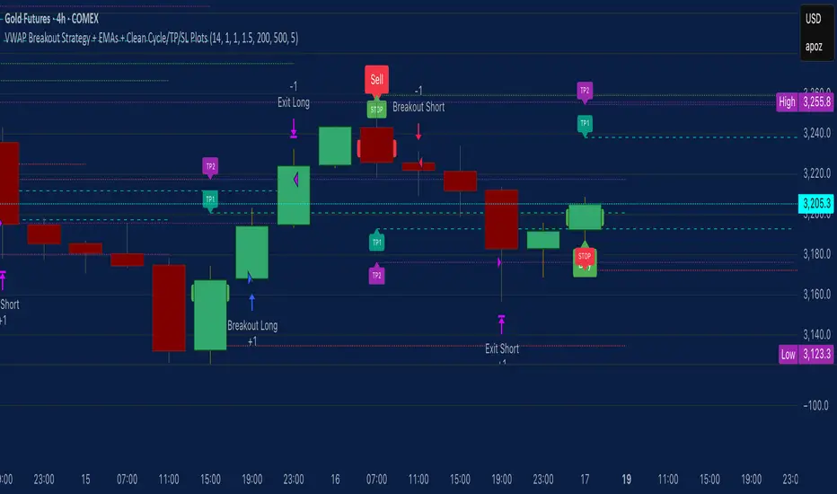
Flux Charts - S&D Automation💎 GENERAL OVERVIEW
The MTF Supply & Demand Zones (S&D) Automation is a powerful and versatile tool designed to help traders rigorously test their trading strategies against historical market data. With various advanced settings, traders can fine-tune their strategies, assess performance, and identify key improvements before deploying in live trading environments. This tool offers a wide range of configurable settings, explained within this write-up.
Features of the new S&D Automation:
Step By Step : Configure your strategy step by step, which will allow you to have OR & AND logic in your strategies.
Highly Configurable : Offers multiple parameters for fine-tuning trade entry and exit conditions.
Multi-Timeframe Analysis : Allows traders to analyze multiple timeframes simultaneously for enhanced accuracy.
Provides advanced stop-loss, take-profit, and break-even settings.
Incorporates Supply & Demand Zone conditions, with settings like Sensitivity, Zone Invalidation, Minimum Zone Width & Minimum Zone Length settings for refined strategy execution.
🚩 UNIQUENESS
The S&D Automation stands out from conventional backtesting tools due to its unparalleled flexibility, precision, and advanced trading logic integration. Key factors that make it unique include:
✅ Comprehensive Strategy Customization – Unlike traditional backtesters that offer basic entry and exit conditions, S&D Automation provides a highly detailed parameter set, allowing traders to fine-tune their strategies with precision.
✅ Multi-Timeframe Supply & Demand Zones – This is the first-ever tool that allows traders to backtest Supply & Demand zones on multiple timeframes.
✅ Customizable Take-Profit Conditions – Offers various methods to set take-profit exits, including using core features from Supply & Demand Zones, and fixed exits like ATR, % change or price change, enabling traders to tailor their exit strategies to specific market behaviors.
✅ Customizable Stop-Loss Conditions – Provides several ways to set up stop losses, including using concepts from Supply & Demand Zones and trailing stops or fixed exits like ATR, % change or price change, allowing for dynamic risk management tailored to individual strategies.
✅ Integration of External Indicators – Allows the inclusion of other indicators or data sources from TradingView for creating strategy conditions, enabling traders to enhance their strategies with additional insights and data points.
By integrating these advanced features, S&D Automation ensures that traders can rigorously test and optimize their strategies with great accuracy and efficiency.
📌 HOW DOES IT WORK ?
The first setting you will want to set it the pyramiding setting. This setting controls the number of simultaneous trades in the same direction allowed in the strategy. For example, if you set it to 1, only one trade can be active in any time, and the second trade will not be entered unless the first one is exited. If it is set to 2, the script will handle both of them at the same time. Note that you should enter the same value to this pyramiding setting, and the pyramiding setting in the "Properties" tab of the script for this to work.
You can enable and set a backtesting window that will limit the entries to between the start date & end date.
Then, you can enter your desired settings for Supply & Demand Zones. You can also enable and set up to 3 timeframes, which you can use later on when customizing your strategies enter / exit conditions.
Entry Conditions
From the "Long Conditions" or the "Short Conditions" groups, you can set your position entry conditions. For settings like "initial capital" or "order size", you can open the "Properties" tab, where these are handled.
The S&D Automation can use the following conditions for entry conditions :
1. Demand Zone
Detection: Triggered when a Demand Zone forms or is detected
Retest: Triggered when price retests a Demand Zone. A retest is confirmed when a candle enters a Demand Zone and closes outside of it.
2nd Retest: Triggered when price retests a Demand Zone for the second time. A retest is confirmed when a candle enters a Demand Zone and closes outside of it.
3rd Retest: Triggered when price retests a Demand Zone for the third time. A retest is confirmed when a candle enters a Demand Zone and closes outside of it.
Retracement: Triggered when price touches a Demand Zone
Break: Triggered when a Demand Zone is invalidated by candle close or wick, depending on the user's input.
2. Supply Zone
Detection: Triggered when a Supply Zone forms or is detected
Retest: Triggered when price retests a Supply Zone. A retest is confirmed when a candle enters a Supply Zone and closes outside of it.
2nd Retest: Triggered when price retests a Supply Zone for the second time. A retest is confirmed when a candle enters a Supply Zone and closes outside of it.
3rd Retest: Triggered when price retests a Supply Zone for the third time. A retest is confirmed when a candle enters a Supply Zone and closes outside of it.
Retracement: Triggered when price touches a Supply Zone
Break: Triggered when a Supply Zone is invalidated by candle close or wick, depending on the user's input.
3. Any Zone
Detection: Triggered when any Supply or Demand Zone forms or is detected
Retest: Triggered when price retests any Supply or Demand Zone. A retest is confirmed when a candle enters any Supply or Demand Zone and closes outside of it.
2nd Retest: Triggered when price retests any Supply or Demand Zone for the second time. A retest is confirmed when a candle enters any Supply or Demand Zone and closes outside of it.
3rd Retest: Triggered when price retests any Supply or Demand Zone for the third time. A retest is confirmed when a candle enters any Supply or Demand Zone and closes outside of it.
Retracement: Triggered when price touches any Supply or Demand Zone
Break: Triggered when any Supply or Demand Zone is invalidated by candle close or wick, depending on the user's input.
🕒 TIMEFRAME CONDITIONS
The S&D Automation supports Multi-Timeframe (MTF) features, just like the Supply & Demand indicator. When setting an entry condition, you can also choose the timeframe.
To set up MTF conditions, navigate to the 'Timeframes' section in the settings, select your desired timeframes, and enable them. You can choose up to three timeframes.
Once you've selected your timeframes, you can use them in your strategy. When setting long and short entry/exit conditions, you can choose from Timeframe 1, Timeframe 2, or Timeframe 3.
External Conditions
Users can use external indicators on the chart to set entry conditions.
The second dropdown in the external condition settings allows you to choose a conditional operator to compare external outputs. Available options include:
Less Than or Equal To: <=
Less Than: <
Equal To: =
Greater Than: >
Greater Than or Equal To: >=
The position entry conditions work like this ;
Each side has 5 S&D Zone conditions and 1 Source condition. Each condition can be enabled or disabled using the checkbox on the left side of them.
The next selection is the alert type, which you can select between "Detection", "Retest", "Retracement" or "Break".
You can select which timeframe this condition should work on from Timeframe 1, 2, or 3. If you select "Any Timeframe", the condition will work for all timeframes.
Lastly select the step of this condition from 1 to 6.
The Source Condition
The last condition on each side is a source condition that is different from the others. Using this condition, you can create your own logic using other indicators' outputs on your chart. For example, suppose that you have an EMA indicator in your chart. You can have the source condition to something like "EMA > high".
The Step System
Each condition has a step number, and conditions are in topological order based on them.
The conditions are executed step by step. This means the condition with step 2 cannot be executed before the condition with step 1 is executed.
Conditions with the same step numbers have "OR" logic. This means that if you have 2 conditions with step 3, the condition with step 4 can trigger after only one of the step 3 conditions is executed.
➕ OTHER ENTRY FEATURES
The S&D Automation allows traders to choose when to execute trades and when not to execute trades.
1. Only Take Trades
This setting lets users specify the time period when their strategy can open or execute trades.
2. Don't Take Trades
This setting lets users specify time periods when their strategy can't open or execute trades.
↩️ EXIT CONDITIONS
1. Exit on Opposite Signal
When enabled, a long position will close when short entry conditions are met, and a short position will close when long entry conditions are met.
2. Exit on Session End
When enabled, positions will be closed at the end of the trading session.
📈 TAKE PROFIT CONDITIONS
There are several methods available for setting take profit exits and conditions.
1. Entry Condition TP
Users can use entry conditions as triggers for take-profit exits. This setting can be found under the long and short exit conditions.
2. Fixed TP
Users can set a fixed TP for exits. This setting can be found under the long and short exit conditions. Users can choose between the following:
Price: This method triggers a TP exit when price reaches a specified level. For example, if you set the Price TP to 10 and buy NASDAQ:TSLA at $190, the trade will automatically exit when the price reaches $200 ($190 + $10).
Ticks: This method triggers a TP exit when price moves a specified number of ticks.
Percentage (%): This method triggers a TP exit when price moves a specified percentage.
ATR: This method triggers a TP exit based on a specified multiple of the Average True Range (ATR).
📉 STOP LOSS CONDITIONS
There are several methods available for setting stop-loss exits and conditions.
1. Entry Condition SL
Users can use entry conditions as triggers for stop-loss exits. This setting can be found under the long and short exit conditions.
2. Fixed SL
Users can set a fixed SL for exits. This setting can be found under the long and short exit conditions. Users can choose between the following:
Price: This method triggers a SL exit when price reaches a specified level. For example, if you set the Price SL to 10 and buy NASDAQ:TSLA at $200, the trade will automatically exit when the price reaches $190 ($200 - $10).
Ticks: This method triggers a SL exit when price moves a specified number of ticks.
Percentage (%): This method triggers a SL exit when price moves a specified percentage.
ATR: This method triggers a SL exit based on a specified multiple of the Average True Range (ATR).
3. Trailing Stop
An explanation & example for the trailing stop feature is present on the write-up within the next section.
Exit conditions have the same logic of constructing conditions like the entry ones. You can construct a Take-Profit Condition & a Stop-Loss Condition. Note that the Take-Profit condition will only work if the position is in profit, regardless of if it's triggered or not. The same applies for the Stop-Loss condition, meaning that it will only work if the position is in loss.
You can also set a Fixed TP & Fixed SL based on the price movement after the position is entered. You have options like "Price", "Ticks", "%", or "Average True Range". For example, you can set a Fixed TP like "5%", and the position will be entered once it moves 5% up in a long position.
Trailing Stop
For the Fixed SL, you also have a "Trailing" stop option, for which you can set its activation level as well. The Trailing stop activation level and its value are expressed in ticks. Check this scenario for an example :
We have a ticker with a tick value of $1. Our Trailing Stop is set to 10 ticks, and the activation level is set to 30 ticks.
We buy 1 contract when the price is $100.
When the price becomes $110, we are in $10 (10 ticks) profit and the trailing stop is now activated.
The current price our stop's on is $110 - $30 (30 ticks), which is the level of $80.
The trailing stop will only move if the price moves up the highest high the price has been after we entered the position.
Let's suppose that price moves up $40 right after our trailing stop is activated. The price will now be $150, and our trailing stop will sit on $150 - $30 (30 ticks) = $120.
If the price is down the $120 level, our stop loss will be triggered.
There is also a "Hard SL" option designed for a backup stop-loss when trailing stops are enabled. You can enable & set this option and if the price goes down before our trailing stop even activates, the position will be exited.
You can also move stop-loss to the break-even (entry price of the position) after a certain profit is achieved using the last setting of the exit conditions. Note that for this to work, you must have a Fixed SL set-up.
➕ OTHER EXIT FEATURES
1. Move Stop Loss to Breakeven
This setting allows the strategy to automatically move the SL to Breakeven (BE) when the position is in profit by a certain amount. Users can choose between the following:
Price: This method moves the SL to BE when price reaches a specified level.
Ticks: This method moves the SL to BE when price moves a specified number of ticks.
Percentage (%): This method moves the SL to BE when price moves a specified percentage.
ATR: This method moves the SL to BE when price moves a specified multiple of the Average True Range (ATR).
Example Entry Scenario
To give an example , check this scenario; out conditions are :
LONG CONDITIONS
Demand Zone Detection, Step 1
Supply Zone Retest, Step 2
Demand Zone Break, Step 2
open > close, Step 3
First, the strategy needs to detect a Demand Zone Detection in order to start working.
After it's detected, now it's looking for either a Supply Zone Retest, or a Demand Zone Break to proceed to the next step, the reason for this is that they both have the same step number.
After one of them is detected, the strategy will consistently check candlesticks for the condition open > close. If a bullish candlestick occurs, a long position will be entered.
⏰ ALERTS
This indicator uses TradingView's strategy alert system. All entries and exits will be sent as an alert if configured. It's possible to further customize these alerts to your liking. For more information check TradingView's strategy alert customization page : www.tradingview.com
⚙️ SETTINGS
1. Backtesting Settings
Pyramiding: Controls the number of simultaneous trades allowed in the strategy. This setting must have the same value that is entered on the script's properties tab on the settings pane.
Enable Custom Backtesting Period: Restricts backtesting to a specific date range.
Start & End Time Configuration: Define precise start and end dates for historical analysis.
2. General Configuration
Detection Method: There are two detection methods you can choose from for identifying Supply & Demand Zones. Both methods aim to identify key areas where price is likely to react, but they do so using different approaches. Traders can choose the method that aligns with their trading style and time horizon.
Sensitivity: The Sensitivity setting allows traders to adjust how aggressively the script identifies supply and demand zones when using the Momentum Detection Method. This setting directly impacts the threshold for detecting zones when using the momentum detection method.
Zone Invalidation: The Zone Invalidation setting determines how supply and demand zones are invalidated.
Wick -> A zone is invalidated if a candle’s wick goes below a demand zone or above a supply zone.
Close -> A zone is invalidated if a candle closes below a demand zone or above a supply zone.
Zone Visibility Range: The Zone Visibility Range setting controls how far from the current price supply and demand zones are displayed on the chart. It helps traders focus on relevant zones while avoiding clutter from distant or less impactful areas.
Minimum Zone Width: The Minimum Zone Width setting defines the smallest size a supply or demand zone must have to be displayed on the chart. It uses the Average True Range (ATR) as a reference to ensure zones are proportionate to current market volatility.
Minimum Zone Length: The Minimum Zone Length setting determines the minimum number of bars a supply or demand zone must span to be displayed on the chart. This setting helps filter out short-lived or insignificant zones, ensuring only meaningful areas of supply or demand are highlighted.
3. Multi-Timeframe Analysis
Enable Up to Three Timeframes: Select and analyze trades across multiple timeframes.
4. Entry Conditions for Long & Short Trades
Multiple Conditions (1-6): Configure up to six independent conditions per trade direction.
Condition Types: Options include Detection, Retest, 2nd Retest, 3rd Retest, Retracement, and Break.
Timeframe Specification: Choose between "Any Timeframe", "Timeframe 1", "Timeframe 2", or "Timeframe 3".
Trade Execution Filters: Restrict trades within specific trading sessions.
5. Exit Conditions for Long & Short Trades
Exit on Opposite Signal: Automatically exit trades upon opposite trade conditions.
Exit on Session End: Closes all positions at the end of the trading session.
Multiple Take-Profit (TP) and Stop-Loss (SL) Configurations:
TP/SL based on % move, ATR, Ticks, or Fixed Price.
Hard SL option for additional risk control.
Move SL to BE (Break Even) after a certain profit threshold.
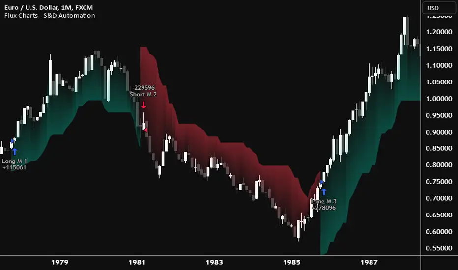
Cracking Cryptocurrency - Bottom Feeder Strategy TesterBottom Feeder - Strategy Tester
The Bottom Feeder is designed to algorithmically detect significantly oversold conditions in price that represent profitable buying opportunities. Combining this with it’s unique Stop and Target System, the Bottom Feeder is designed to return consistent return with minimal draw down. Whether used as a Market Bottom Detector or as a system for executing safe, profitable mean reversion trades, the Bottom Feeder is a powerful tool in any trader’s arsenal.
Bottom Feeder was designed to be used on BTCUSD, however it is also effective on other USD/USDT pairs. One will have to check the individual pair they wish to trade with the Strategy Tester to simulate performance.
Strategy displayed is from 2018-2021 on **Conservative Mode** with Percent of Equity (30%) enabled.
Options
Let’s go through the input options one by one, so that you are able to comfortably navigate all that this indicator has to offer. The link below will display a picture of the layout of the settings for your convenience.
For the sake of simplicity, let’s note now that all settings marked **Conservative Mode** will not work in Aggressive Mode.
Mode : Determines how aggressively Bottom Feeder generates a buy signal. In Conservative Mode, trades can only be opened once per candle and the stop and target will update as new signals appear. In Aggressive Mode, a separate trade is opened each time Bottom Feeder signals, which may be multiple times within one Daily candle.
Position Sizing Strategy : Determines what Risk Management system you will deploy when trading Bottom Feeder. Your options are “Percent of Equity” and “Distance to Stop Loss”. If Percent of Equity is selected, a trade size will be equal to a percentage of your equity, pursuant to the value in the ‘Percent of Equity’ box. If Distance to Stop Loss is selected, then your Position Size will be determined based off the distance to your stop loss and the value in the ‘Risk Percentage’ box.
Percent Of Equity : Determines what percentage of your equity will be allocated to each trade when ‘Position Sizing Strategy’ is enabled.
Risk Percentage : Determines the size of each trade if ‘Distance to Stop Loss’ strategy is enabled. This value reflects what percent of your account you will lose per trade if the trade hits your stop loss.
Plot Target and Stop Loss : Toggles on/off the visualized take profit and stop losses on the chart.
**Conservative Mode** TP Multiplier : This is an input box, it requires a float value. That is, it can accept either a whole number integer or a number with a decimal. This number will determine your Take Profit target. It will take whatever number is entered into this box and multiply the Average True Range against it to determine your Take Profit.
**Conservative Mode** SL Multiplier : See above - this will modify your Stop Loss Value.
**Conservative Mode** Average or Median True Range : This is a drop-down option, the two options are Average True Range or Median True Range. If Average True Range is selected, then this indicator will use the Average True Range calculation, that is, the average of a historical set of True Range values to determine the Average True Range value for Target and Stop Loss calculation. If Median True Range is selected, it will not take an average and will instead take the Median value of your historical look back period.
**Conservative Mode** True Range Length : This is an input that requires an integer. This will represent your historical lookback period for Average/Median True Range calculation.
**Conservative Mode** True Range Smoothing : This is a drop-down with the following options: Exponential Moving Average ( EMA ), Simple Moving Average ( SMA ), Weighted Moving Average ( WMA ), Relative Moving Average (RMA). This will determine the smoothing type for calculating the Average True Range if it is selected. Note: if Median True Range is selected above, this option will not have any effect as there is no smoothing for a Median value.
**Conservative Mode** Custom True Range Value? : This is a true/false option that is false by default. If enabled, it will override the Average/Median True Range calculation in favor of a users custom True Range value to be input below.
**Conservative Mode** Custom True Range Value : This is an input box that requires a float value. If Custom True Range is enabled this is where a user will input their desired custom True Range value for Target and Stop Loss calculation.
From Month/Day/Year to Month/Day/Year : This sets the Time Frame of your backtest for the Bottom Feeder Strategy. It will run FROM the date selected TO the date selected.
Stop and Target Description
Because Bottom Feeder is designed only to scalp the various market bottoms that can appear over time in the market and not to identify trends or to trade ranges, it’s imperative that the indicator notify us not just to when to enter our trades, but when to exit! In the service of that, CC Bottom Feeder has a built in Stop and Target system that tracks and displays the stop loss and take profit levels of each individual open trade, whether in Aggressive or Conservative Mode.
Conservative Mode Targeting: In Conservative Mode, Bottom Feeder signals are aggregated into a compound trade. The signal will appear as a green label pointing up below a candle, and will appear upon a candle close. If Bottom Feeder then generates another signal the stop loss and target price will be updated. The process will continue until the aggregated trade completes in either direction. On a trade with multiple signals, a larger position is slowly entered into upon each buy signal.
Aggressive Mode Targeting: In Aggressive Mode, Bottom Feeder signals are individually displayed as they are generated, regardless of how many signals are generated on any single candle. If Bottom Feeder continues to signal, each individual open trade will have their own stop loss and target that will be displayed on the chart until the individual trade completes in either direction. As opposed to a large compound position, aggressive mode represents a higher number of independent signals with their own stop and target levels.
Stop losses and targets are designed to be hard, not soft. That is, they are intended to be stop market orders, not mental stop losses. If price wicks through the target or stop, it will activate.
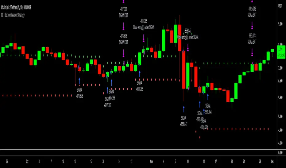
saodisengxiaoyu-lianghua-2.1- This indicator is a modular, signal-building framework designed to generate long and short signals by combining a chosen leading indicator with selectable confirmation filters. It runs on Pine Script version 5, overlays directly on price, and is built to be highly configurable so traders can tailor the signal logic to their market, timeframe, and trading style. It includes a dashboard to visualize which conditions are active and whether they validate a signal, and it outputs clear buy/sell labels and alert conditions so you can automate or monitor trades with confidence.
Core Design
- Leading Indicator: You choose one primary signal generator from a broad list (for example, Range Filter, Supertrend, MACD, RSI, Ichimoku, and many others). This serves as the anchor of the system and determines when a preliminary long or short setup exists.
- Confirmation Filters: You can enable additional filters that validate the leading signal before it becomes actionable. Each “respect…” input toggles a filter on or off. These filters include popular tools like EMA, 2/3 EMA crosses, RQK (Nadaraya Watson), ADX/DMI, Bollinger-based oscillators, MACD variations, QQE, Hull, VWAP, Choppiness Index, Damiani Volatility, and more.
- Signal Expiry: To avoid waiting indefinitely for confirmations, the indicator counts how many consecutive bars the leading condition holds. If confirmations do not align within a defined number of bars, the setup expires. This controls latency and helps reduce late or stale entries.
- Alternating Signals: An optional mode enforces alternation (long must follow short and vice versa), helping avoid repeated entries in the same direction without a meaningful reset.
- Aggregation Logic: The final long/short conditions are formed by combining the leading condition with all selected confirmation filters through logical conjunction. Only if all enabled filters validate the signal (within expiry constraints) does the indicator consider it a confirmed long or short.
- Visualization and Alerts: The script plots buy/sell labels at signal points, provides alert conditions for automation, and displays a compact dashboard summarizing the leading indicator’s status and each confirmation’s pass/fail result using checkmarks.
Leading Indicator Options
- The indicator includes a very large menu of leading tools, each with its own logic to determine uptrend or downtrend impulses. Highlights include:
- Range Filter: Uses a dynamic centerline and bands computed via conditional EMA/SMA and range sizing to define directional movement. It can operate in a default mode or an alternative “DW” mode.
- Rational Quadratic Kernel (RQK): Applies a kernel smoothing model (Nadaraya Watson) to detect uptrends and downtrends with a focus on noise reduction.
- Supertrend, Half Trend, SSL Channel: Classic trend-following tools that derive direction from ATR-based bands or moving average channels.
- Ichimoku Cloud and SuperIchi: Multi-component systems validating trend via cloud position, conversion/base line relationships, projected cloud, and lagging span.
- TSI (True Strength Index), DPO (Detrended Price Oscillator), AO (Awesome Oscillator), MACD, STC (Schaff Trend Cycle), QQE Mod: Momentum and cycle tools that parse direction from crossovers, zero-line behavior, and momentum shifts.
- Donchian Trend Ribbon, Chandelier Exit: Trend and exit tools that can validate breakouts or sustained trend strength.
- ADX/DMI: Measures trend strength and directional movement via +DI/-DI relationships and minimum ADX thresholds.
- RSI and Stochastic: Use crossovers, level exits, or threshold filters to gate entries based on overbought/oversold dynamics or relative strength trends.
- Vortex, Chaikin Money Flow, VWAP, Bull Bear Power, ROC, Wolfpack Id, Hull Suite: A diverse set of directional, momentum, and volume-based indicators to suit different markets and styles.
- Trendline Breakout and Range Detector: Price-behavior filters that confirm signals during breakouts or within defined ranges.
Confirmation Filters
- Each filter is optional. When enabled, it must validate the leading condition for a signal to pass. Examples:
- EMA Filter: Requires price to be above a specified EMA for longs and below for shorts, filtering signals that contradict broader trend or baseline levels.
- 2 EMA Cross and 3 EMA Cross: Enforce moving average cross conditions (fast above slow for long, the reverse for short) or a three-line stacking logic for more stringent trend alignment.
- RQK, Supertrend, Half Trend, Donchian, QQE, Hull, MACD (crossover vs. zero-line), AO (zero line or AC momentum variants), SSL: Each adds its characteristic validation pattern.
- RSI family (MA cross, exits OB/OS zones, threshold levels) plus RSI MA direction and RSI/RSI MA limits: Multiple ways to constrain signals via relative strength behavior and trajectories.
- Choppiness Index and Damiani Volatility: Prevent entries during ranging conditions or insufficient volatility; choppiness thresholds and volatility states gate the trade.
- VWAP, Volume modes (above MA, simple up/down, delta), Chaikin Money Flow: Volume and flow conditions that ensure signals happen in supportive liquidity or accumulation/distribution contexts.
- ADX/DMI thresholds: Demand a minimum trend strength and directional DI alignment to reduce whipsaw trades.
- Trendline Breakout and Range Detector: Confirm that the price is breaking structure or remains within active range consistent with the leading setup.
- By combining several filters you can create strict, conservative entries or looser setups depending on your goals.
Range Filter Engine
- A core building block, the Range Filter uses conditional EMA and SMA functions to compute adaptive bands around a dynamic centerline. It supports two types:
- Type 1: The centerline updates when price exceeds the band thresholds; bands define acceptable drift ranges.
- Type 2: Uses quantized steps (via floor operations) relative to the previous centerline to handle larger moves in discrete increments.
- The engine offers smoothing for range values using a secondary EMA and can switch between raw and averaged outputs. Its hi/lo bands and centerline compose a corridor that defines directional movement and potential breakout confirmation.
Signal Construction
- The script computes:
- leadinglongcond and leadingshortcond : The primary directional signals from the chosen leading indicator.
- longCond and shortCond : Final signals formed by combining the leading conditions with all enabled confirmations. Each confirmation contributes a boolean gate. If a filter is disabled, it contributes a neutral pass-through, keeping the logic intact without enforcing that condition.
- Expiry Logic: The code counts consecutive bars where the leading condition remains true. If confirmations do not line up within the user-defined “Signal Expiry Candle Count,” the setup is abandoned and the signal does not trigger.
- Alternation: An optional state ensures that long and short signals alternate. This can reduce repeated entries in the same direction without a clear reset.
- Finally, longCondition and shortCondition represent the actionable signals after expiry and alternation logic. These drive the label plotting and alert conditions.
Visualization
- Buy and Sell Labels: When longCondition or shortCondition confirm, the script plots annotated labels directly on the chart, making entries easy to see at a glance. The labels use color coding and clear text tags (“long” vs. “short”).
- Dashboard: A table summarizes the status of the leading indicator and all confirmations. Each row shows the indicator label and whether it passed (✔️) or failed (❌) on the current bar. This intensely practical UI helps you diagnose why a signal did or did not trigger, empowering faster strategy iteration and parameter tuning.
- Failed Confirmation Markers: If a setup expires (count exceeds the limit) and confirmations failed to align, the script can mark the chart with a small label and provide a tooltip listing which confirmations did not pass. It’s a helpful audit trail to understand missed trades or prevent “chasing” invalid signals.
- Data Window Values: The script outputs signal states to the data window, which can be useful for debugging or building composite conditions in multi-indicator templates.
Inputs and Parameters
- You control the indicator from a comprehensive input panel:
- Setup: Signal expiry count, whether to enforce alternating signals, and whether to display labels and the dashboard (including position and size).
- Leading Indicator: Choose the primary signal generator from the large list.
- Per-Filter Toggles: For each confirmation, a respect... toggle enables or disables it. Many include sub-options (like MACD type, Stochastic mode, RSI mode, ADX variants, thresholds for choppiness/volatility, etc.) to fine-tune behavior.
- Range Filter Settings: Choose type and behavior; select default vs. DW mode and smoothing. The underlying functions adjust band sizes using ATR, average change, standard deviation, or user-defined scales.
- Because everything is customizable, you can adapt the indicator to different assets, volatility regimes, and timeframes.
Alerts and Automation
- The script defines alert conditions tied to longCondition and shortCondition . You can set these alerts in your chart to trigger notifications or webhook calls for automated execution in external bots. The alert text is simple, and you can configure your own message template when creating alerts in the chart, including JSON payloads for algorithmic integration.
Typical Workflow
- Select a Leading Indicator aligned with your style. For trend following, Supertrend or SSL may be appropriate; for momentum, MACD or TSI; for range/trend-change detection, Range Filter, RQK, or Donchian.
- Add a few key Confirmation Filters that complement the leading signal. For example:
- Pair Supertrend with EMA Filter and RSI MA Direction to ensure trend alignment and positive momentum.
- Combine MACD Crossover with ADX/DMI and Volume Above MA to avoid signals in low-trend or low-liquidity conditions.
- Use RQK with Choppiness Index and Damiani Volatility to only act when the market is trending and volatile enough.
- Set a sensible Signal Expiry Candle Count. Shorter expiry keeps entries timely and reduces lag; longer expiry captures setups that mature slowly.
- Observe the Dashboard during live markets to see which filters pass or fail, then iterate. Tighten or loosen thresholds and filter combinations as needed.
- For automation, turn on alerts for the final conditions and use webhook payloads to notify your trading robot.
Strengths and Practical Notes
- Flexibility: The indicator is a toolkit rather than a single rigid model. It lets you test different combinations rapidly and visualize outcomes immediately.
- Clarity: Labels, dashboard, and failed-confirmation markers make it easy to audit behavior and refine settings without digging into code.
- Robustness: The expiry and alternation options add discipline, avoiding the temptation to enter late or repeatedly in one direction without a reset.
- Modular Design: The logical gates (“respect…”) make the behavior transparent: if a filter is on, it must pass; if it’s off, the signal ignores it. This keeps reasoning clean.
- Avoiding Overfitting: Because you can stack many filters, it’s tempting to over-constrain signals. Start simple (one leading indicator and one or two confirmations). Add complexity only if it demonstrably improves your edge across varied market regimes.
Limitations and Recommendations
- No single configuration is universally optimal. Markets change; tune filters for the instrument and timeframe you trade and revisit settings periodically.
- Trend filters can underperform in choppy markets; likewise, momentum filters can false-trigger in quiet periods. Consider using Choppiness Index or Damiani to gate signals by regime.
- Use expiry wisely. Too short may miss good setups that need a few bars to confirm; too long may cause late entries. Balance responsiveness and accuracy.
- Always consider risk management externally (position sizing, stops, profit targets). The indicator focuses on signal quality; combining it with robust trade management methods will improve results.
Example Configurations
- Trend-Following Setup:
- Leading: Supertrend uptrend for longs and downtrend for shorts.
- Confirmations: EMA Filter (price above 200 EMA for long, below for short), ADX/DMI (trend strength above threshold with +DI/-DI alignment), Volume Above MA.
- Expiry: 3–4 bars to keep entries timely.
- Result: Strong bias toward sustained moves while avoiding weak trends and thin liquidity.
- Mean-Reversion to Momentum Crossover:
- Leading: RSI exits from OB/OS zones (e.g., RSI leaves oversold for long and leaves overbought for short).
- Confirmations: 2 EMA Cross (fast crossing slow in the same direction), MACD zero-line behavior for added momentum validation.
- Expiry: 2–3 bars for responsive re-entry.
- Result: Captures momentum transitions after short-term extremes, with extra confirmation to reduce head-fakes.
- Range Breakout Focus:
- Leading: Range Filter Type 2 or Donchian Trend Ribbon to detect breakouts.
- Confirmations: Damiani Volatility (avoid low-volatility false breaks), Choppiness Index (prefer trend-ready states), ROC positive/negative threshold.
- Expiry: 1–3 bars to act on breakout windows.
- Result: Better alignment to breakout dynamics, gating trades by volatility and regime.
Conclusion
- This indicator is a comprehensive, configurable framework that merges a chosen leading signal with an array of corroborating filters, disciplined expiry handling, and intuitive visualization. It’s designed to help you build high-quality entry signals tailored to your approach, whether that’s trend-following, breakout trading, momentum capturing, or a hybrid. By surfacing pass/fail states in a dashboard and allowing alert-based automation, it bridges the gap between discretionary analysis and systematic execution. With sensible parameter tuning and thoughtful filter selection, it can serve as a robust backbone for signal generation across diverse instruments and timeframes.

多指标量化交易DIY- The indicator includes a very large menu of leading tools, each with its own logic to determine uptrend or downtrend impulses. Highlights include:
- Range Filter: Uses a dynamic centerline and bands computed via conditional EMA/SMA and range sizing to define directional movement. It can operate in a default mode or an alternative “DW” mode.
- Rational Quadratic Kernel (RQK): Applies a kernel smoothing model (Nadaraya Watson) to detect uptrends and downtrends with a focus on noise reduction.
- Supertrend, Half Trend, SSL Channel: Classic trend-following tools that derive direction from ATR-based bands or moving average channels.
- Ichimoku Cloud and SuperIchi: Multi-component systems validating trend via cloud position, conversion/base line relationships, projected cloud, and lagging span.
- TSI (True Strength Index), DPO (Detrended Price Oscillator), AO (Awesome Oscillator), MACD, STC (Schaff Trend Cycle), QQE Mod: Momentum and cycle tools that parse direction from crossovers, zero-line behavior, and momentum shifts.
- Donchian Trend Ribbon, Chandelier Exit: Trend and exit tools that can validate breakouts or sustained trend strength.
- ADX/DMI: Measures trend strength and directional movement via +DI/-DI relationships and minimum ADX thresholds.
- RSI and Stochastic: Use crossovers, level exits, or threshold filters to gate entries based on overbought/oversold dynamics or relative strength trends.
- Vortex, Chaikin Money Flow, VWAP, Bull Bear Power, ROC, Wolfpack Id, Hull Suite: A diverse set of directional, momentum, and volume-based indicators to suit different markets and styles.
- Trendline Breakout and Range Detector: Price-behavior filters that confirm signals during breakouts or within defined ranges.
Confirmation Filters
- Each filter is optional. When enabled, it must validate the leading condition for a signal to pass. Examples:
- EMA Filter: Requires price to be above a specified EMA for longs and below for shorts, filtering signals that contradict broader trend or baseline levels.
- 2 EMA Cross and 3 EMA Cross: Enforce moving average cross conditions (fast above slow for long, the reverse for short) or a three-line stacking logic for more stringent trend alignment.
- RQK, Supertrend, Half Trend, Donchian, QQE, Hull, MACD (crossover vs. zero-line), AO (zero line or AC momentum variants), SSL: Each adds its characteristic validation pattern.
- RSI family (MA cross, exits OB/OS zones, threshold levels) plus RSI MA direction and RSI/RSI MA limits: Multiple ways to constrain signals via relative strength behavior and trajectories.
- Choppiness Index and Damiani Volatility: Prevent entries during ranging conditions or insufficient volatility; choppiness thresholds and volatility states gate the trade.
- VWAP, Volume modes (above MA, simple up/down, delta), Chaikin Money Flow: Volume and flow conditions that ensure signals happen in supportive liquidity or accumulation/distribution contexts.
- ADX/DMI thresholds: Demand a minimum trend strength and directional DI alignment to reduce whipsaw trades.
- Trendline Breakout and Range Detector: Confirm that the price is breaking structure or remains within active range consistent with the leading setup.
- By combining several filters you can create strict, conservative entries or looser setups depending on your goals.
Range Filter Engine
- A core building block, the Range Filter uses conditional EMA and SMA functions to compute adaptive bands around a dynamic centerline. It supports two types:
- Type 1: The centerline updates when price exceeds the band thresholds; bands define acceptable drift ranges.
- Type 2: Uses quantized steps (via floor operations) relative to the previous centerline to handle larger moves in discrete increments.
- The engine offers smoothing for range values using a secondary EMA and can switch between raw and averaged outputs. Its hi/lo bands and centerline compose a corridor that defines directional movement and potential breakout confirmation.
Signal Construction
- The script computes:
- leadinglongcond and leadingshortcond : The primary directional signals from the chosen leading indicator.
- longCond and shortCond : Final signals formed by combining the leading conditions with all enabled confirmations. Each confirmation contributes a boolean gate. If a filter is disabled, it contributes a neutral pass-through, keeping the logic intact without enforcing that condition.
- Expiry Logic: The code counts consecutive bars where the leading condition remains true. If confirmations do not line up within the user-defined “Signal Expiry Candle Count,” the setup is abandoned and the signal does not trigger.
- Alternation: An optional state ensures that long and short signals alternate. This can reduce repeated entries in the same direction without a clear reset.
- Finally, longCondition and shortCondition represent the actionable signals after expiry and alternation logic. These drive the label plotting and alert conditions.
Visualization
- Buy and Sell Labels: When longCondition or shortCondition confirm, the script plots annotated labels directly on the chart, making entries easy to see at a glance. The labels use color coding and clear text tags (“long” vs. “short”).
- Dashboard: A table summarizes the status of the leading indicator and all confirmations. Each row shows the indicator label and whether it passed (✔️) or failed (❌) on the current bar. This intensely practical UI helps you diagnose why a signal did or did not trigger, empowering faster strategy iteration and parameter tuning.
- Failed Confirmation Markers: If a setup expires (count exceeds the limit) and confirmations failed to align, the script can mark the chart with a small label and provide a tooltip listing which confirmations did not pass. It’s a helpful audit trail to understand missed trades or prevent “chasing” invalid signals.
- Data Window Values: The script outputs signal states to the data window, which can be useful for debugging or building composite conditions in multi-indicator templates.
Inputs and Parameters
- You control the indicator from a comprehensive input panel:
- Setup: Signal expiry count, whether to enforce alternating signals, and whether to display labels and the dashboard (including position and size).
- Leading Indicator: Choose the primary signal generator from the large list.
- Per-Filter Toggles: For each confirmation, a respect... toggle enables or disables it. Many include sub-options (like MACD type, Stochastic mode, RSI mode, ADX variants, thresholds for choppiness/volatility, etc.) to fine-tune behavior.
- Range Filter Settings: Choose type and behavior; select default vs. DW mode and smoothing. The underlying functions adjust band sizes using ATR, average change, standard deviation, or user-defined scales.
- Because everything is customizable, you can adapt the indicator to different assets, volatility regimes, and timeframes.
Alerts and Automation
- The script defines alert conditions tied to longCondition and shortCondition . You can set these alerts in your chart to trigger notifications or webhook calls for automated execution in external bots. The alert text is simple, and you can configure your own message template when creating alerts in the chart, including JSON payloads for algorithmic integration.
Typical Workflow
- Select a Leading Indicator aligned with your style. For trend following, Supertrend or SSL may be appropriate; for momentum, MACD or TSI; for range/trend-change detection, Range Filter, RQK, or Donchian.
- Add a few key Confirmation Filters that complement the leading signal. For example:
- Pair Supertrend with EMA Filter and RSI MA Direction to ensure trend alignment and positive momentum.
- Combine MACD Crossover with ADX/DMI and Volume Above MA to avoid signals in low-trend or low-liquidity conditions.
- Use RQK with Choppiness Index and Damiani Volatility to only act when the market is trending and volatile enough.
- Set a sensible Signal Expiry Candle Count. Shorter expiry keeps entries timely and reduces lag; longer expiry captures setups that mature slowly.
- Observe the Dashboard during live markets to see which filters pass or fail, then iterate. Tighten or loosen thresholds and filter combinations as needed.
- For automation, turn on alerts for the final conditions and use webhook payloads to notify your trading robot.
Strengths and Practical Notes
- Flexibility: The indicator is a toolkit rather than a single rigid model. It lets you test different combinations rapidly and visualize outcomes immediately.
- Clarity: Labels, dashboard, and failed-confirmation markers make it easy to audit behavior and refine settings without digging into code.
- Robustness: The expiry and alternation options add discipline, avoiding the temptation to enter late or repeatedly in one direction without a reset.
- Modular Design: The logical gates (“respect…”) make the behavior transparent: if a filter is on, it must pass; if it’s off, the signal ignores it. This keeps reasoning clean.
- Avoiding Overfitting: Because you can stack many filters, it’s tempting to over-constrain signals. Start simple (one leading indicator and one or two confirmations). Add complexity only if it demonstrably improves your edge across varied market regimes.
Limitations and Recommendations
- No single configuration is universally optimal. Markets change; tune filters for the instrument and timeframe you trade and revisit settings periodically.
- Trend filters can underperform in choppy markets; likewise, momentum filters can false-trigger in quiet periods. Consider using Choppiness Index or Damiani to gate signals by regime.
- Use expiry wisely. Too short may miss good setups that need a few bars to confirm; too long may cause late entries. Balance responsiveness and accuracy.
- Always consider risk management externally (position sizing, stops, profit targets). The indicator focuses on signal quality; combining it with robust trade management methods will improve results.
Example Configurations
- Trend-Following Setup:
- Leading: Supertrend uptrend for longs and downtrend for shorts.
- Confirmations: EMA Filter (price above 200 EMA for long, below for short), ADX/DMI (trend strength above threshold with +DI/-DI alignment), Volume Above MA.
- Expiry: 3–4 bars to keep entries timely.
- Result: Strong bias toward sustained moves while avoiding weak trends and thin liquidity.
- Mean-Reversion to Momentum Crossover:
- Leading: RSI exits from OB/OS zones (e.g., RSI leaves oversold for long and leaves overbought for short).
- Confirmations: 2 EMA Cross (fast crossing slow in the same direction), MACD zero-line behavior for added momentum validation.
- Expiry: 2–3 bars for responsive re-entry.
- Result: Captures momentum transitions after short-term extremes, with extra confirmation to reduce head-fakes.
- Range Breakout Focus:
- Leading: Range Filter Type 2 or Donchian Trend Ribbon to detect breakouts.
- Confirmations: Damiani Volatility (avoid low-volatility false breaks), Choppiness Index (prefer trend-ready states), ROC positive/negative threshold.
- Expiry: 1–3 bars to act on breakout windows.
- Result: Better alignment to breakout dynamics, gating trades by volatility and regime.
Conclusion
- This indicator is a comprehensive, configurable framework that merges a chosen leading signal with an array of corroborating filters, disciplined expiry handling, and intuitive visualization. It’s designed to help you build high-quality entry signals tailored to your approach, whether that’s trend-following, breakout trading, momentum capturing, or a hybrid. By surfacing pass/fail states in a dashboard and allowing alert-based automation, it bridges the gap between discretionary analysis and systematic execution. With sensible parameter tuning and thoughtful filter selection, it can serve as a robust backbone for signal generation across diverse instruments and timeframes.
