Wave Conflict DetectorWave Conflict Detector
Wave Conflict Detector: Identifying Pivot Conditions Through Wave Interference Analysis
Wave Conflict Detector applies wave interference principles from physics to dual-EMA analysis, identifying potential pivot conditions by measuring phase relationships and amplitude states between two moving average waves. Unlike traditional EMA crossover systems that signal on wave intersection, this indicator measures the directional alignment (phase) and interaction strength (interference amplitude) between wave states to identify conditions where wave mechanics suggest potential reversal zones.
The indicator combines two analytical components: velocity-based phase difference calculation that measures whether waves are moving in the same or opposite directions, and normalized interference amplitude that quantifies the degree of wave reinforcement or cancellation. This creates a regime-classification system with visual feedback showing when waves are aligned (constructive state) versus opposed (destructive state).
What Makes This Approach Different
Phase Relationship Measurement
The core analytical method is extracting phase alignment from wave velocities rather than simply measuring EMA separation. The system calculates the first derivative (bar-to-bar change) of each EMA, creating velocity measurements: v₁ = ψ₁ - ψ₁ and v₂ = ψ₂ - ψ₂ . These velocities are combined through normalized correlation: Φ = (v₁ × v₂) / |v|², producing an alignment value ranging from -1 (perfect opposition) to +1 (perfect alignment).
This alignment value is smoothed using EMA and converted to angular degrees: Δφ = (1 - Φ) × 90°, creating a phase difference measurement from 0° to 180°. This quantifies how much the waves are "fighting" each other directionally, independent of their separation distance. Two EMAs can be far apart yet moving in harmony (low phase difference), or close together yet moving in opposition (high phase difference).
This directional correlation approach differs from standard dual-EMA analysis by focusing on velocity alignment rather than positional crossovers.
Interference Amplitude Calculation
The interference formula implements wave superposition principles: I = (|ψ₁ + ψ₂|² - |ψ₁ - ψ₂|²) × Gain, which mathematically simplifies to I = 4 × ψ₁ × ψ₂ × Gain. This measures the product of both waves—when both are positive and large, interference is maximally constructive; when they have opposite signs or differing magnitudes, interference weakens.
The raw interference value is then normalized using adaptive statistical bounds calculated over a rolling window (default 100 bars). The system computes mean (μ) and standard deviation (σ) of raw interference, then applies bounds of μ ± 2σ, and normalizes to a 0-1 range. This creates a scale-invariant measurement that adapts automatically to different instruments and volatility regimes without requiring manual recalibration.
The combination of phase measurement and normalized amplitude creates a two-dimensional state space for classifying market conditions.
Dual-Mode Detection Architecture
The system offers two detection approaches that can be selected based on market conditions:
Interference Mode: Detects pivot conditions when normalized interference amplitude forms local peaks or troughs (current bar is higher/lower than both adjacent bars) AND exceeds the configured threshold. This identifies extremes in wave interaction strength.
Phase Mode: Detects pivot conditions when phase alignment reverses (crosses from positive to negative or vice versa) AND absolute phase difference exceeds the threshold. This identifies directional relationship changes between waves.
Both modes require price structure confirmation (traditional pivot high/low patterns) and minimum bar spacing to prevent over-signaling. This architecture allows traders to match detection sensitivity to market character—interference mode for amplitude-driven markets, phase mode for directional trend shifts.
Multi-Layer Visual System
The visualization approach uses hierarchical layers to display wave state information:
Foundation Layer: The two EMA waves (ψ₁ and ψ₂) plotted directly on the price chart, showing the underlying wave states being analyzed.
Background Layer: Color-coded zones showing regime state—green tint when phase alignment is positive (constructive interference), red tint when phase alignment is negative below -0.3 (destructive interference).
Dynamic Ribbon: A band centered on the wave average with width proportional to |ψ₁ - ψ₂| × (0.5 + interference_norm). This creates an adaptive channel that expands with interference strength and contracts during low-energy states.
Phase Field: Multi-frequency harmonic oscillations generated using three phase accumulators driven by interference amplitude, phase alignment, and accumulated phase rotation. Multiple sine-wave layers create visual texture that becomes erratic during wave conflict conditions and smooth during aligned states.
Particle System: Floating symbols whose density is proportional to interference amplitude, creating a visual intensity indicator.
Each visual component displays non-redundant information about the wave state system.
Core Calculation Methodology
Wave State Generation
Two exponential moving averages are calculated using configurable lengths (default 8 and 21 bars):
- ψ₁ = EMA(close, fastLen) — fast wave component
- ψ₂ = EMA(close, slowLen) — slow wave component
These serve as the base wave functions for all subsequent analysis.
Velocity Extraction
First derivatives are computed as simple bar-to-bar differences:
- psi1_velocity = ψ₁ - ψ₁
- psi2_velocity = ψ₂ - ψ₂
These represent the "motion" of each wave through price-time space.
Phase Alignment Calculation
The velocity product and magnitude are calculated:
- velocity_product = v₁ × v₂
- velocity_magnitude = √(v₁² + v₂²)
Phase alignment is computed as:
- phase_alignment = velocity_product / (velocity_magnitude²)
This is smoothed using EMA of configurable length (default 5) and converted to degrees:
- phase_degrees = (1 - phase_alignment_smooth) × 90
Interference Amplitude Processing
Raw interference is calculated:
- interference_raw = (constructive_amplitude - destructive_amplitude) × gain
- where constructive_amplitude = (ψ₁ + ψ₂)²
- and destructive_amplitude = (ψ₁ - ψ₂)²
Statistical normalization is applied:
- interference_mean = SMA(interference_raw, normalizationLen)
- interference_std = StdDev(interference_raw, normalizationLen)
- upper_bound = mean + 2 × std
- lower_bound = mean - 2 × std
- interference_norm = (interference_raw - lower_bound) / (upper_bound - lower_bound), clamped to
State Classification
Three regime states are identified:
- Constructive: phase_alignment_smooth > 0 (waves moving in same direction)
- Destructive: phase_alignment_smooth < -0.3 (waves moving in opposite directions)
- Neutral: phase_alignment between -0.3 and 0 (weak directional correlation)
Pivot Detection Logic
In Interference Mode:
- High pivots: interference_norm > interference_norm AND interference_norm > interference_norm AND interference_norm > threshold AND price forms pivot high AND spacing requirement met
- Low pivots: interference_norm shows local trough using opposite conditions
In Phase Mode:
- Pivots: phase alignment reverses sign AND absolute phase_degrees > threshold AND price forms pivot high/low AND spacing requirement met
All conditions must be true for a signal to generate.
Dashboard Metrics System
The dashboard displays real-time calculations:
- I (Interference): Normalized amplitude shown as bar gauge and percentage
- Δφ (Phase): Phase difference shown as bar gauge and degrees
- ψ₁ and ψ₂: Current wave values in price units
- Wave Separation: |ψ₁ - ψ₂| with directional indicator
- STATE: Current regime classification (CONSTRUCTIVE/DESTRUCTIVE/NEUTRAL)
- PIVOT Probability: Composite score calculated as interference_norm × (phase_degrees/180) × 100
The interference matrix shows historical heatmap data across four metrics (interference amplitude, phase difference, constructive flags, destructive flags) over the configurable number of bars.
How to Use This Indicator
Initial Configuration
Apply the indicator to your chart with default settings. The fast wave length (default 8) should be adjusted to match short-term price swings for your instrument and timeframe. The slow wave length (default 21) should be 2-4 times the fast length to create adequate wave separation. Enable the dashboard (recommended position: top right) to monitor regime state and metrics in real-time.
Signal Interpretation
High Pivot Marker (▼ Red Triangle): Appears above price bars when a bearish pivot condition is detected. This indicates that price formed a swing high, the selected detection criteria were met (interference peak or phase reversal depending on mode), threshold requirements were satisfied, and the minimum spacing filter passed. This represents a potential reversal zone where wave mechanics suggest downward directional change conditions.
Low Pivot Marker (▲ Green Triangle): Appears below price bars when a bullish pivot condition is detected. This indicates that price formed a swing low and all detection criteria aligned. This represents a potential reversal zone where wave mechanics suggest upward directional change conditions.
Dashboard STATE Reading
The STATE field shows current wave relationship:
- "🟢 CONSTRUCTIVE": Waves are moving in the same direction (phase alignment positive). This suggests trend continuation conditions where waves are reinforcing each other.
- "🔴 DESTRUCTIVE": Waves are moving in opposite directions (phase alignment below -0.3). This suggests reversal-prone conditions where waves are conflicting.
- "🟡 NEUTRAL": Weak directional correlation between waves. This suggests ranging or transitional conditions.
Use STATE for regime awareness rather than specific entry signals.
Interference and Phase Metrics
Monitor the I (Interference) percentage:
- Above 70%: High amplitude state, significant wave interaction
- 40-70%: Moderate amplitude state
- Below 40%: Low amplitude state, weak interaction
Monitor the Δφ (Phase) degrees:
- Above 120°: Significant wave opposition (destructive conditions)
- 60-120°: Transitional phase relationship
- Below 60°: Wave alignment (constructive conditions)
The PIVOT probability metric combines both: high values (>70%) indicate conditions where both amplitude and phase suggest elevated pivot formation potential.
Trading Workflow Example
Step 1 - Regime Check: Observe dashboard STATE to understand current wave relationship. CONSTRUCTIVE states favor trend-following approaches, DESTRUCTIVE states suggest reversal-prone conditions.
Step 2 - Metric Monitoring: Watch I% and Δφ values. Rising interference with high phase difference indicates building wave conflict.
Step 3 - Visual Confirmation: Observe amplitude ribbon width (expanding = active state) and phase field texture (chaotic = conflict conditions, smooth = aligned conditions).
Step 4 - Signal Wait: Wait for confirmed pivot marker (▼ or ▲) rather than anticipating based on metrics alone. The marker indicates all detection criteria have aligned.
Step 5 - Entry Decision: Use pivot markers as potential reversal zones. Combine with other analysis methods such as support/resistance levels, volume confirmation, and higher timeframe bias for entry decisions.
Step 6 - Risk Management: Place stops beyond recent swing structure or ribbon edges. Monitor dashboard STATE—if it flips to CONSTRUCTIVE in trade direction, the reversal may be confirmed; if PIVOT% drops significantly, conditions may be weakening.
Step 7 - Exit Criteria: Consider exits when opposite pivot marker appears, STATE changes unfavorably, or standard technical targets are reached.
Parameter Optimization Guidelines
Fast Wave Length: Adjust to match short-term swing frequency. Shorter values (5-8) for active trading on lower timeframes, longer values (13-20) for swing trading on higher timeframes.
Slow Wave Length: Should maintain 2-4x ratio with fast length. Shorter values create more interference cycles, longer values create more stable baseline.
Phase Detection Length: Smoothing for phase alignment. Lower values (3-5) for responsive detection, higher values (8-12) for stable readings with less sensitivity.
Interference Gain: Amplification multiplier. Lower values (0.5-1.0) for conservative detection, higher values (1.5-2.5) for more sensitive detection.
Normalization Period: Rolling window for statistical bounds. Shorter periods (50-100) adapt quickly to volatility changes, longer periods (150-300) provide more stable normalization.
Interference Threshold: Minimum amplitude to trigger signals. Lower values (0.50-0.60) generate more signals, higher values (0.70-0.85) are more selective.
Phase Threshold: Minimum phase difference in degrees. Lower values (90-110) are more permissive, higher values (140-170) require stronger opposition.
Min Pivot Spacing: Bars between signals. Match to average swing duration on your timeframe—tighter spacing (3-8 bars) for scalping, wider spacing (15-30 bars) for swing trading.
Best Performance Conditions
This approach works better in markets with:
- Clear swing structure where EMA-based wave analysis is meaningful
- Sufficient volatility for wave separation to develop
- Periodic oscillation between trending and ranging states
- Liquid instruments where EMAs reflect true price flow
This approach may be less effective in:
- Extremely choppy conditions with no directional persistence
- Very low volatility environments where wave separation is minimal
- Gap-heavy instruments where price discontinuities disrupt wave continuity
- Parabolic moves where waves cannot keep pace with price velocity
The system adapts by reducing signal frequency in poor conditions—when interference stays below threshold or phase alignment remains neutral, pivot markers will not appear.
Visual Performance Optimization
The phase field and particle systems are computationally intensive. If experiencing chart lag:
- Reduce Phase Field Layers from 5 to 2-3 (significant performance improvement)
- Lower Particle Density from 3 to 1 (reduces label creation overhead)
- Disable Phase Field entirely (removes most intensive calculations)
- Decrease Matrix History Bars to 15-20 (reduces table computation load)
The core wave analysis and pivot detection continue to function with all visual elements disabled.
Important Disclaimers
This indicator is an analytical tool that measures phase relationships and interference amplitude between two exponential moving averages. It identifies conditions where these wave mechanics suggest potential pivot zones based on historical price data analysis. It should not be used as a standalone trading system.
The phase and interference calculations are deterministic mathematical formulas applied to EMA values. These measurements describe current and historical wave relationships but do not predict future price movements. Past wave patterns and pivot markers do not guarantee future market behavior will follow similar patterns.
All trading involves risk. The pivot markers represent analytical conditions where wave mechanics align with specific thresholds, not certainty of directional change. Use appropriate risk management, position sizing, and combine with additional confirmation methods such as support/resistance analysis, volume patterns, and multi-timeframe alignment. No indicator can eliminate false signals or guarantee profitable trades.
The spacing filter and threshold requirements are designed to reduce noise and over-signaling, but market conditions can change rapidly and render any analytical signal invalid. Always use stop losses and never risk capital you cannot afford to lose.
Technical Implementation Notes
All calculations execute on closed bars only—there is no repainting of signals or values. The normalization system requires approximately 100 bars of historical data to establish stable statistical bounds; values in the first 50-100 bars may be unstable as the rolling statistics converge.
Phase field arrays are fixed-size based on the complexity setting. Particle labels are capped at 80 total to prevent excessive memory usage. Dashboard and matrix tables update only on the last bar to minimize computational overhead. Particle generation is throttled to every 2 bars for performance. Phase accumulators use modulo arithmetic (% 2π) to prevent numerical overflow during extended operation.
The indicator has been tested across multiple timeframes (5-minute through daily) and multiple asset classes (forex, stocks, crypto, indices). It functions identically across all instruments due to the adaptive normalization approach.
Search in scripts for "swing trading"

Liquidity Sweep & Reversal — Body Anchored + Risk (v6)Overview
The Liquidity Sweep & Reversal — Locked to Price (v6) indicator identifies liquidity sweeps around major swing highs and lows, confirming reversals when price closes back inside the swept level.
All signals are locked to price (bottom of green candle for BUY, top of red candle for SELL), so they remain perfectly aligned when zooming or scaling.
This indicator is ideal for swing traders and scalpers who trade reversals, liquidity events, and reclaim structures.
How It Works
Detects confirmed swing highs and lows using a pivot-based structure.
Waits for a liquidity sweep — when price wicks beyond a recent swing.
Confirms a reclaim when price closes back inside the previous swing level.
Triggers a BUY or SELL signal anchored to the candle body.
Automatically calculates stop loss and risk using ATR and your inputs.
Input Settings
Swing Detection
Swing Detection Strength: How many bars confirm a swing pivot. Higher = stronger swings.
Bars to Confirm Reclaim: Number of bars after a sweep for price to close back within the swing zone.
Swing Proximity %: How close price must come to a swing to count as a liquidity sweep.
Trend Filter (optional)
Use EMA Trend Filter: When enabled, only BUY in uptrend and SELL in downtrend.
Fast EMA Length / Slow EMA Length: Define EMAs used to detect trend direction.
Risk & Stop Management
ATR Length: Period for ATR calculation (volatility measurement).
Base ATR Stop Buffer (x ATR): Distance of stop loss from entry based on ATR multiplier.
Position Size (quote units): Your total position size in quote currency (e.g., USDT).
Risk % of (Position / 20): Defines how much of your position to risk per trade.
Example: (Position / 20) × Risk % = per-trade risk.
Chart Elements
BUY Arrow (green): Appears after a liquidity sweep and reclaim near a swing low.
SELL Arrow (red): Appears after a sweep and reclaim near a swing high.
Labels: Display entry price, stop loss (SL), and calculated risk dollar value.
EMAs: Optional fast/slow moving averages for directional bias.
Dynamic Stops: Adjust automatically using ATR × risk settings.
Trading Tips
Use BUY signals near liquidity sweeps under swing lows.
Use SELL signals near liquidity sweeps above swing highs.
Adjust swing length for different timeframes:
Lower values for scalping (3–5)
Higher values for swing trading (7–10)
Respect stop loss levels and use risk control settings for consistent sizing.
Combine with volume, OBV, or structure for confirmation.
Alerts
BUY — Locked to Price: "BUY: swing low reclaimed with dynamic stop."
SELL — Locked to Price: "SELL: swing high reclaimed with dynamic stop."
Best Use Cases
Liquidity-based reversals
Swing entry confirmation
Stop hunt reclaims
Structure-based entries
Author
Created by @roccodallas
For traders who value clean structure, risk control, and chart precision.

Quantum Rotational Field MappingQuantum Rotational Field Mapping (QRFM):
Phase Coherence Detection Through Complex-Plane Oscillator Analysis
Quantum Rotational Field Mapping applies complex-plane mathematics and phase-space analysis to oscillator ensembles, identifying high-probability trend ignition points by measuring when multiple independent oscillators achieve phase coherence. Unlike traditional multi-oscillator approaches that simply stack indicators or use boolean AND/OR logic, this system converts each oscillator into a rotating phasor (vector) in the complex plane and calculates the Coherence Index (CI) —a mathematical measure of how tightly aligned the ensemble has become—then generates signals only when alignment, phase direction, and pairwise entanglement all converge.
The indicator combines three mathematical frameworks: phasor representation using analytic signal theory to extract phase and amplitude from each oscillator, coherence measurement using vector summation in the complex plane to quantify group alignment, and entanglement analysis that calculates pairwise phase agreement across all oscillator combinations. This creates a multi-dimensional confirmation system that distinguishes between random oscillator noise and genuine regime transitions.
What Makes This Original
Complex-Plane Phasor Framework
This indicator implements classical signal processing mathematics adapted for market oscillators. Each oscillator—whether RSI, MACD, Stochastic, CCI, Williams %R, MFI, ROC, or TSI—is first normalized to a common scale, then converted into a complex-plane representation using an in-phase (I) and quadrature (Q) component. The in-phase component is the oscillator value itself, while the quadrature component is calculated as the first difference (derivative proxy), creating a velocity-aware representation.
From these components, the system extracts:
Phase (φ) : Calculated as φ = atan2(Q, I), representing the oscillator's position in its cycle (mapped to -180° to +180°)
Amplitude (A) : Calculated as A = √(I² + Q²), representing the oscillator's strength or conviction
This mathematical approach is fundamentally different from simply reading oscillator values. A phasor captures both where an oscillator is in its cycle (phase angle) and how strongly it's expressing that position (amplitude). Two oscillators can have the same value but be in opposite phases of their cycles—traditional analysis would see them as identical, while QRFM sees them as 180° out of phase (contradictory).
Coherence Index Calculation
The core innovation is the Coherence Index (CI) , borrowed from physics and signal processing. When you have N oscillators, each with phase φₙ, you can represent each as a unit vector in the complex plane: e^(iφₙ) = cos(φₙ) + i·sin(φₙ).
The CI measures what happens when you sum all these vectors:
Resultant Vector : R = Σ e^(iφₙ) = Σ cos(φₙ) + i·Σ sin(φₙ)
Coherence Index : CI = |R| / N
Where |R| is the magnitude of the resultant vector and N is the number of active oscillators.
The CI ranges from 0 to 1:
CI = 1.0 : Perfect coherence—all oscillators have identical phase angles, vectors point in the same direction, creating maximum constructive interference
CI = 0.0 : Complete decoherence—oscillators are randomly distributed around the circle, vectors cancel out through destructive interference
0 < CI < 1 : Partial alignment—some clustering with some scatter
This is not a simple average or correlation. The CI captures phase synchronization across the entire ensemble simultaneously. When oscillators phase-lock (align their cycles), the CI spikes regardless of their individual values. This makes it sensitive to regime transitions that traditional indicators miss.
Dominant Phase and Direction Detection
Beyond measuring alignment strength, the system calculates the dominant phase of the ensemble—the direction the resultant vector points:
Dominant Phase : φ_dom = atan2(Σ sin(φₙ), Σ cos(φₙ))
This gives the "average direction" of all oscillator phases, mapped to -180° to +180°:
+90° to -90° (right half-plane): Bullish phase dominance
+90° to +180° or -90° to -180° (left half-plane): Bearish phase dominance
The combination of CI magnitude (coherence strength) and dominant phase angle (directional bias) creates a two-dimensional signal space. High CI alone is insufficient—you need high CI plus dominant phase pointing in a tradeable direction. This dual requirement is what separates QRFM from simple oscillator averaging.
Entanglement Matrix and Pairwise Coherence
While the CI measures global alignment, the entanglement matrix measures local pairwise relationships. For every pair of oscillators (i, j), the system calculates:
E(i,j) = |cos(φᵢ - φⱼ)|
This represents the phase agreement between oscillators i and j:
E = 1.0 : Oscillators are in-phase (0° or 360° apart)
E = 0.0 : Oscillators are in quadrature (90° apart, orthogonal)
E between 0 and 1 : Varying degrees of alignment
The system counts how many oscillator pairs exceed a user-defined entanglement threshold (e.g., 0.7). This entangled pairs count serves as a confirmation filter: signals require not just high global CI, but also a minimum number of strong pairwise agreements. This prevents false ignitions where CI is high but driven by only two oscillators while the rest remain scattered.
The entanglement matrix creates an N×N symmetric matrix that can be visualized as a web—when many cells are bright (high E values), the ensemble is highly interconnected. When cells are dark, oscillators are moving independently.
Phase-Lock Tolerance Mechanism
A complementary confirmation layer is the phase-lock detector . This calculates the maximum phase spread across all oscillators:
For all pairs (i,j), compute angular distance: Δφ = |φᵢ - φⱼ|, wrapping at 180°
Max Spread = maximum Δφ across all pairs
If max spread < user threshold (e.g., 35°), the ensemble is considered phase-locked —all oscillators are within a narrow angular band.
This differs from entanglement: entanglement measures pairwise cosine similarity (magnitude of alignment), while phase-lock measures maximum angular deviation (tightness of clustering). Both must be satisfied for the highest-conviction signals.
Multi-Layer Visual Architecture
QRFM includes six visual components that represent the same underlying mathematics from different perspectives:
Circular Orbit Plot : A polar coordinate grid showing each oscillator as a vector from origin to perimeter. Angle = phase, radius = amplitude. This is a real-time snapshot of the complex plane. When vectors converge (point in similar directions), coherence is high. When scattered randomly, coherence is low. Users can see phase alignment forming before CI numerically confirms it.
Phase-Time Heat Map : A 2D matrix with rows = oscillators and columns = time bins. Each cell is colored by the oscillator's phase at that time (using a gradient where color hue maps to angle). Horizontal color bands indicate sustained phase alignment over time. Vertical color bands show moments when all oscillators shared the same phase (ignition points). This provides historical pattern recognition.
Entanglement Web Matrix : An N×N grid showing E(i,j) for all pairs. Cells are colored by entanglement strength—bright yellow/gold for high E, dark gray for low E. This reveals which oscillators are driving coherence and which are lagging. For example, if RSI and MACD show high E but Stochastic shows low E with everything, Stochastic is the outlier.
Quantum Field Cloud : A background color overlay on the price chart. Color (green = bullish, red = bearish) is determined by dominant phase. Opacity is determined by CI—high CI creates dense, opaque cloud; low CI creates faint, nearly invisible cloud. This gives an atmospheric "feel" for regime strength without looking at numbers.
Phase Spiral : A smoothed plot of dominant phase over recent history, displayed as a curve that wraps around price. When the spiral is tight and rotating steadily, the ensemble is in coherent rotation (trending). When the spiral is loose or erratic, coherence is breaking down.
Dashboard : A table showing real-time metrics: CI (as percentage), dominant phase (in degrees with directional arrow), field strength (CI × average amplitude), entangled pairs count, phase-lock status (locked/unlocked), quantum state classification ("Ignition", "Coherent", "Collapse", "Chaos"), and collapse risk (recent CI change normalized to 0-100%).
Each component is independently toggleable, allowing users to customize their workspace. The orbit plot is the most essential—it provides intuitive, visual feedback on phase alignment that no numerical dashboard can match.
Core Components and How They Work Together
1. Oscillator Normalization Engine
The foundation is creating a common measurement scale. QRFM supports eight oscillators:
RSI : Normalized from to using overbought/oversold levels (70, 30) as anchors
MACD Histogram : Normalized by dividing by rolling standard deviation, then clamped to
Stochastic %K : Normalized from using (80, 20) anchors
CCI : Divided by 200 (typical extreme level), clamped to
Williams %R : Normalized from using (-20, -80) anchors
MFI : Normalized from using (80, 20) anchors
ROC : Divided by 10, clamped to
TSI : Divided by 50, clamped to
Each oscillator can be individually enabled/disabled. Only active oscillators contribute to phase calculations. The normalization removes scale differences—a reading of +0.8 means "strongly bullish" regardless of whether it came from RSI or TSI.
2. Analytic Signal Construction
For each active oscillator at each bar, the system constructs the analytic signal:
In-Phase (I) : The normalized oscillator value itself
Quadrature (Q) : The bar-to-bar change in the normalized value (first derivative approximation)
This creates a 2D representation: (I, Q). The phase is extracted as:
φ = atan2(Q, I) × (180 / π)
This maps the oscillator to a point on the unit circle. An oscillator at the same value but rising (positive Q) will have a different phase than one that is falling (negative Q). This velocity-awareness is critical—it distinguishes between "at resistance and stalling" versus "at resistance and breaking through."
The amplitude is extracted as:
A = √(I² + Q²)
This represents the distance from origin in the (I, Q) plane. High amplitude means the oscillator is far from neutral (strong conviction). Low amplitude means it's near zero (weak/transitional state).
3. Coherence Calculation Pipeline
For each bar (or every Nth bar if phase sample rate > 1 for performance):
Step 1 : Extract phase φₙ for each of the N active oscillators
Step 2 : Compute complex exponentials: Zₙ = e^(i·φₙ·π/180) = cos(φₙ·π/180) + i·sin(φₙ·π/180)
Step 3 : Sum the complex exponentials: R = Σ Zₙ = (Σ cos φₙ) + i·(Σ sin φₙ)
Step 4 : Calculate magnitude: |R| = √
Step 5 : Normalize by count: CI_raw = |R| / N
Step 6 : Smooth the CI: CI = SMA(CI_raw, smoothing_window)
The smoothing step (default 2 bars) removes single-bar noise spikes while preserving structural coherence changes. Users can adjust this to control reactivity versus stability.
The dominant phase is calculated as:
φ_dom = atan2(Σ sin φₙ, Σ cos φₙ) × (180 / π)
This is the angle of the resultant vector R in the complex plane.
4. Entanglement Matrix Construction
For all unique pairs of oscillators (i, j) where i < j:
Step 1 : Get phases φᵢ and φⱼ
Step 2 : Compute phase difference: Δφ = φᵢ - φⱼ (in radians)
Step 3 : Calculate entanglement: E(i,j) = |cos(Δφ)|
Step 4 : Store in symmetric matrix: matrix = matrix = E(i,j)
The matrix is then scanned: count how many E(i,j) values exceed the user-defined threshold (default 0.7). This count is the entangled pairs metric.
For visualization, the matrix is rendered as an N×N table where cell brightness maps to E(i,j) intensity.
5. Phase-Lock Detection
Step 1 : For all unique pairs (i, j), compute angular distance: Δφ = |φᵢ - φⱼ|
Step 2 : Wrap angles: if Δφ > 180°, set Δφ = 360° - Δφ
Step 3 : Find maximum: max_spread = max(Δφ) across all pairs
Step 4 : Compare to tolerance: phase_locked = (max_spread < tolerance)
If phase_locked is true, all oscillators are within the specified angular cone (e.g., 35°). This is a boolean confirmation filter.
6. Signal Generation Logic
Signals are generated through multi-layer confirmation:
Long Ignition Signal :
CI crosses above ignition threshold (e.g., 0.80)
AND dominant phase is in bullish range (-90° < φ_dom < +90°)
AND phase_locked = true
AND entangled_pairs >= minimum threshold (e.g., 4)
Short Ignition Signal :
CI crosses above ignition threshold
AND dominant phase is in bearish range (φ_dom < -90° OR φ_dom > +90°)
AND phase_locked = true
AND entangled_pairs >= minimum threshold
Collapse Signal :
CI at bar minus CI at current bar > collapse threshold (e.g., 0.55)
AND CI at bar was above 0.6 (must collapse from coherent state, not from already-low state)
These are strict conditions. A high CI alone does not generate a signal—dominant phase must align with direction, oscillators must be phase-locked, and sufficient pairwise entanglement must exist. This multi-factor gating dramatically reduces false signals compared to single-condition triggers.
Calculation Methodology
Phase 1: Oscillator Computation and Normalization
On each bar, the system calculates the raw values for all enabled oscillators using standard Pine Script functions:
RSI: ta.rsi(close, length)
MACD: ta.macd() returning histogram component
Stochastic: ta.stoch() smoothed with ta.sma()
CCI: ta.cci(close, length)
Williams %R: ta.wpr(length)
MFI: ta.mfi(hlc3, length)
ROC: ta.roc(close, length)
TSI: ta.tsi(close, short, long)
Each raw value is then passed through a normalization function:
normalize(value, overbought_level, oversold_level) = 2 × (value - oversold) / (overbought - oversold) - 1
This maps the oscillator's typical range to , where -1 represents extreme bearish, 0 represents neutral, and +1 represents extreme bullish.
For oscillators without fixed ranges (MACD, ROC, TSI), statistical normalization is used: divide by a rolling standard deviation or fixed divisor, then clamp to .
Phase 2: Phasor Extraction
For each normalized oscillator value val:
I = val (in-phase component)
Q = val - val (quadrature component, first difference)
Phase calculation:
phi_rad = atan2(Q, I)
phi_deg = phi_rad × (180 / π)
Amplitude calculation:
A = √(I² + Q²)
These values are stored in arrays: osc_phases and osc_amps for each oscillator n.
Phase 3: Complex Summation and Coherence
Initialize accumulators:
sum_cos = 0
sum_sin = 0
For each oscillator n = 0 to N-1:
phi_rad = osc_phases × (π / 180)
sum_cos += cos(phi_rad)
sum_sin += sin(phi_rad)
Resultant magnitude:
resultant_mag = √(sum_cos² + sum_sin²)
Coherence Index (raw):
CI_raw = resultant_mag / N
Smoothed CI:
CI = SMA(CI_raw, smoothing_window)
Dominant phase:
phi_dom_rad = atan2(sum_sin, sum_cos)
phi_dom_deg = phi_dom_rad × (180 / π)
Phase 4: Entanglement Matrix Population
For i = 0 to N-2:
For j = i+1 to N-1:
phi_i = osc_phases × (π / 180)
phi_j = osc_phases × (π / 180)
delta_phi = phi_i - phi_j
E = |cos(delta_phi)|
matrix_index_ij = i × N + j
matrix_index_ji = j × N + i
entangle_matrix = E
entangle_matrix = E
if E >= threshold:
entangled_pairs += 1
The matrix uses flat array storage with index mapping: index(row, col) = row × N + col.
Phase 5: Phase-Lock Check
max_spread = 0
For i = 0 to N-2:
For j = i+1 to N-1:
delta = |osc_phases - osc_phases |
if delta > 180:
delta = 360 - delta
max_spread = max(max_spread, delta)
phase_locked = (max_spread < tolerance)
Phase 6: Signal Evaluation
Ignition Long :
ignition_long = (CI crosses above threshold) AND
(phi_dom > -90 AND phi_dom < 90) AND
phase_locked AND
(entangled_pairs >= minimum)
Ignition Short :
ignition_short = (CI crosses above threshold) AND
(phi_dom < -90 OR phi_dom > 90) AND
phase_locked AND
(entangled_pairs >= minimum)
Collapse :
CI_prev = CI
collapse = (CI_prev - CI > collapse_threshold) AND (CI_prev > 0.6)
All signals are evaluated on bar close. The crossover and crossunder functions ensure signals fire only once when conditions transition from false to true.
Phase 7: Field Strength and Visualization Metrics
Average Amplitude :
avg_amp = (Σ osc_amps ) / N
Field Strength :
field_strength = CI × avg_amp
Collapse Risk (for dashboard):
collapse_risk = (CI - CI) / max(CI , 0.1)
collapse_risk_pct = clamp(collapse_risk × 100, 0, 100)
Quantum State Classification :
if (CI > threshold AND phase_locked):
state = "Ignition"
else if (CI > 0.6):
state = "Coherent"
else if (collapse):
state = "Collapse"
else:
state = "Chaos"
Phase 8: Visual Rendering
Orbit Plot : For each oscillator, convert polar (phase, amplitude) to Cartesian (x, y) for grid placement:
radius = amplitude × grid_center × 0.8
x = radius × cos(phase × π/180)
y = radius × sin(phase × π/180)
col = center + x (mapped to grid coordinates)
row = center - y
Heat Map : For each oscillator row and time column, retrieve historical phase value at lookback = (columns - col) × sample_rate, then map phase to color using a hue gradient.
Entanglement Web : Render matrix as table cell with background color opacity = E(i,j).
Field Cloud : Background color = (phi_dom > -90 AND phi_dom < 90) ? green : red, with opacity = mix(min_opacity, max_opacity, CI).
All visual components render only on the last bar (barstate.islast) to minimize computational overhead.
How to Use This Indicator
Step 1 : Apply QRFM to your chart. It works on all timeframes and asset classes, though 15-minute to 4-hour timeframes provide the best balance of responsiveness and noise reduction.
Step 2 : Enable the dashboard (default: top right) and the circular orbit plot (default: middle left). These are your primary visual feedback tools.
Step 3 : Optionally enable the heat map, entanglement web, and field cloud based on your preference. New users may find all visuals overwhelming; start with dashboard + orbit plot.
Step 4 : Observe for 50-100 bars to let the indicator establish baseline coherence patterns. Markets have different "normal" CI ranges—some instruments naturally run higher or lower coherence.
Understanding the Circular Orbit Plot
The orbit plot is a polar grid showing oscillator vectors in real-time:
Center point : Neutral (zero phase and amplitude)
Each vector : A line from center to a point on the grid
Vector angle : The oscillator's phase (0° = right/east, 90° = up/north, 180° = left/west, -90° = down/south)
Vector length : The oscillator's amplitude (short = weak signal, long = strong signal)
Vector label : First letter of oscillator name (R = RSI, M = MACD, etc.)
What to watch :
Convergence : When all vectors cluster in one quadrant or sector, CI is rising and coherence is forming. This is your pre-signal warning.
Scatter : When vectors point in random directions (360° spread), CI is low and the market is in a non-trending or transitional regime.
Rotation : When the cluster rotates smoothly around the circle, the ensemble is in coherent oscillation—typically seen during steady trends.
Sudden flips : When the cluster rapidly jumps from one side to the opposite (e.g., +90° to -90°), a phase reversal has occurred—often coinciding with trend reversals.
Example: If you see RSI, MACD, and Stochastic all pointing toward 45° (northeast) with long vectors, while CCI, TSI, and ROC point toward 40-50° as well, coherence is high and dominant phase is bullish. Expect an ignition signal if CI crosses threshold.
Reading Dashboard Metrics
The dashboard provides numerical confirmation of what the orbit plot shows visually:
CI : Displays as 0-100%. Above 70% = high coherence (strong regime), 40-70% = moderate, below 40% = low (poor conditions for trend entries).
Dom Phase : Angle in degrees with directional arrow. ⬆ = bullish bias, ⬇ = bearish bias, ⬌ = neutral.
Field Strength : CI weighted by amplitude. High values (> 0.6) indicate not just alignment but strong alignment.
Entangled Pairs : Count of oscillator pairs with E > threshold. Higher = more confirmation. If minimum is set to 4, you need at least 4 pairs entangled for signals.
Phase Lock : 🔒 YES (all oscillators within tolerance) or 🔓 NO (spread too wide).
State : Real-time classification:
🚀 IGNITION: CI just crossed threshold with phase-lock
⚡ COHERENT: CI is high and stable
💥 COLLAPSE: CI has dropped sharply
🌀 CHAOS: Low CI, scattered phases
Collapse Risk : 0-100% scale based on recent CI change. Above 50% warns of imminent breakdown.
Interpreting Signals
Long Ignition (Blue Triangle Below Price) :
Occurs when CI crosses above threshold (e.g., 0.80)
Dominant phase is in bullish range (-90° to +90°)
All oscillators are phase-locked (within tolerance)
Minimum entangled pairs requirement met
Interpretation : The oscillator ensemble has transitioned from disorder to coherent bullish alignment. This is a high-probability long entry point. The multi-layer confirmation (CI + phase direction + lock + entanglement) ensures this is not a single-oscillator whipsaw.
Short Ignition (Red Triangle Above Price) :
Same conditions as long, but dominant phase is in bearish range (< -90° or > +90°)
Interpretation : Coherent bearish alignment has formed. High-probability short entry.
Collapse (Circles Above and Below Price) :
CI has dropped by more than the collapse threshold (e.g., 0.55) over a 5-bar window
CI was previously above 0.6 (collapsing from coherent state)
Interpretation : Phase coherence has broken down. If you are in a position, this is an exit warning. If looking to enter, stand aside—regime is transitioning.
Phase-Time Heat Map Patterns
Enable the heat map and position it at bottom right. The rows represent individual oscillators, columns represent time bins (most recent on left).
Pattern: Horizontal Color Bands
If a row (e.g., RSI) shows consistent color across columns (say, green for several bins), that oscillator has maintained stable phase over time. If all rows show horizontal bands of similar color, the entire ensemble has been phase-locked for an extended period—this is a strong trending regime.
Pattern: Vertical Color Bands
If a column (single time bin) shows all cells with the same or very similar color, that moment in time had high coherence. These vertical bands often align with ignition signals or major price pivots.
Pattern: Rainbow Chaos
If cells are random colors (red, green, yellow mixed with no pattern), coherence is low. The ensemble is scattered. Avoid trading during these periods unless you have external confirmation.
Pattern: Color Transition
If you see a row transition from red to green (or vice versa) sharply, that oscillator has phase-flipped. If multiple rows do this simultaneously, a regime change is underway.
Entanglement Web Analysis
Enable the web matrix (default: opposite corner from heat map). It shows an N×N grid where N = number of active oscillators.
Bright Yellow/Gold Cells : High pairwise entanglement. For example, if the RSI-MACD cell is bright gold, those two oscillators are moving in phase. If the RSI-Stochastic cell is bright, they are entangled as well.
Dark Gray Cells : Low entanglement. Oscillators are decorrelated or in quadrature.
Diagonal : Always marked with "—" because an oscillator is always perfectly entangled with itself.
How to use :
Scan for clustering: If most cells are bright, coherence is high across the board. If only a few cells are bright, coherence is driven by a subset (e.g., RSI and MACD are aligned, but nothing else is—weak signal).
Identify laggards: If one row/column is entirely dark, that oscillator is the outlier. You may choose to disable it or monitor for when it joins the group (late confirmation).
Watch for web formation: During low-coherence periods, the matrix is mostly dark. As coherence builds, cells begin lighting up. A sudden "web" of connections forming visually precedes ignition signals.
Trading Workflow
Step 1: Monitor Coherence Level
Check the dashboard CI metric or observe the orbit plot. If CI is below 40% and vectors are scattered, conditions are poor for trend entries. Wait.
Step 2: Detect Coherence Building
When CI begins rising (say, from 30% to 50-60%) and you notice vectors on the orbit plot starting to cluster, coherence is forming. This is your alert phase—do not enter yet, but prepare.
Step 3: Confirm Phase Direction
Check the dominant phase angle and the orbit plot quadrant where clustering is occurring:
Clustering in right half (0° to ±90°): Bullish bias forming
Clustering in left half (±90° to 180°): Bearish bias forming
Verify the dashboard shows the corresponding directional arrow (⬆ or ⬇).
Step 4: Wait for Signal Confirmation
Do not enter based on rising CI alone. Wait for the full ignition signal:
CI crosses above threshold
Phase-lock indicator shows 🔒 YES
Entangled pairs count >= minimum
Directional triangle appears on chart
This ensures all layers have aligned.
Step 5: Execute Entry
Long : Blue triangle below price appears → enter long
Short : Red triangle above price appears → enter short
Step 6: Position Management
Initial Stop : Place stop loss based on your risk management rules (e.g., recent swing low/high, ATR-based buffer).
Monitoring :
Watch the field cloud density. If it remains opaque and colored in your direction, the regime is intact.
Check dashboard collapse risk. If it rises above 50%, prepare for exit.
Monitor the orbit plot. If vectors begin scattering or the cluster flips to the opposite side, coherence is breaking.
Exit Triggers :
Collapse signal fires (circles appear)
Dominant phase flips to opposite half-plane
CI drops below 40% (coherence lost)
Price hits your profit target or trailing stop
Step 7: Post-Exit Analysis
After exiting, observe whether a new ignition forms in the opposite direction (reversal) or if CI remains low (transition to range). Use this to decide whether to re-enter, reverse, or stand aside.
Best Practices
Use Price Structure as Context
QRFM identifies when coherence forms but does not specify where price will go. Combine ignition signals with support/resistance levels, trendlines, or chart patterns. For example:
Long ignition near a major support level after a pullback: high-probability bounce
Long ignition in the middle of a range with no structure: lower probability
Multi-Timeframe Confirmation
Open QRFM on two timeframes simultaneously:
Higher timeframe (e.g., 4-hour): Use CI level to determine regime bias. If 4H CI is above 60% and dominant phase is bullish, the market is in a bullish regime.
Lower timeframe (e.g., 15-minute): Execute entries on ignition signals that align with the higher timeframe bias.
This prevents counter-trend trades and increases win rate.
Distinguish Between Regime Types
High CI, stable dominant phase (State: Coherent) : Trending market. Ignitions are continuation signals; collapses are profit-taking or reversal warnings.
Low CI, erratic dominant phase (State: Chaos) : Ranging or choppy market. Avoid ignition signals or reduce position size. Wait for coherence to establish.
Moderate CI with frequent collapses : Whipsaw environment. Use wider stops or stand aside.
Adjust Parameters to Instrument and Timeframe
Crypto/Forex (high volatility) : Lower ignition threshold (0.65-0.75), lower CI smoothing (2-3), shorter oscillator lengths (7-10).
Stocks/Indices (moderate volatility) : Standard settings (threshold 0.75-0.85, smoothing 5-7, oscillator lengths 14).
Lower timeframes (5-15 min) : Reduce phase sample rate to 1-2 for responsiveness.
Higher timeframes (daily+) : Increase CI smoothing and oscillator lengths for noise reduction.
Use Entanglement Count as Conviction Filter
The minimum entangled pairs setting controls signal strictness:
Low (1-2) : More signals, lower quality (acceptable if you have other confirmation)
Medium (3-5) : Balanced (recommended for most traders)
High (6+) : Very strict, fewer signals, highest quality
Adjust based on your trade frequency preference and risk tolerance.
Monitor Oscillator Contribution
Use the entanglement web to see which oscillators are driving coherence. If certain oscillators are consistently dark (low E with all others), they may be adding noise. Consider disabling them. For example:
On low-volume instruments, MFI may be unreliable → disable MFI
On strongly trending instruments, mean-reversion oscillators (Stochastic, RSI) may lag → reduce weight or disable
Respect the Collapse Signal
Collapse events are early warnings. Price may continue in the original direction for several bars after collapse fires, but the underlying regime has weakened. Best practice:
If in profit: Take partial or full profit on collapse
If at breakeven/small loss: Exit immediately
If collapse occurs shortly after entry: Likely a false ignition; exit to avoid drawdown
Collapses do not guarantee immediate reversals—they signal uncertainty .
Combine with Volume Analysis
If your instrument has reliable volume:
Ignitions with expanding volume: Higher conviction
Ignitions with declining volume: Weaker, possibly false
Collapses with volume spikes: Strong reversal signal
Collapses with low volume: May just be consolidation
Volume is not built into QRFM (except via MFI), so add it as external confirmation.
Observe the Phase Spiral
The spiral provides a quick visual cue for rotation consistency:
Tight, smooth spiral : Ensemble is rotating coherently (trending)
Loose, erratic spiral : Phase is jumping around (ranging or transitional)
If the spiral tightens, coherence is building. If it loosens, coherence is dissolving.
Do Not Overtrade Low-Coherence Periods
When CI is persistently below 40% and the state is "Chaos," the market is not in a regime where phase analysis is predictive. During these times:
Reduce position size
Widen stops
Wait for coherence to return
QRFM's strength is regime detection. If there is no regime, the tool correctly signals "stand aside."
Use Alerts Strategically
Set alerts for:
Long Ignition
Short Ignition
Collapse
Phase Lock (optional)
Configure alerts to "Once per bar close" to avoid intrabar repainting and noise. When an alert fires, manually verify:
Orbit plot shows clustering
Dashboard confirms all conditions
Price structure supports the trade
Do not blindly trade alerts—use them as prompts for analysis.
Ideal Market Conditions
Best Performance
Instruments :
Liquid, actively traded markets (major forex pairs, large-cap stocks, major indices, top-tier crypto)
Instruments with clear cyclical oscillator behavior (avoid extremely illiquid or manipulated markets)
Timeframes :
15-minute to 4-hour: Optimal balance of noise reduction and responsiveness
1-hour to daily: Slower, higher-conviction signals; good for swing trading
5-minute: Acceptable for scalping if parameters are tightened and you accept more noise
Market Regimes :
Trending markets with periodic retracements (where oscillators cycle through phases predictably)
Breakout environments (coherence forms before/during breakout; collapse occurs at exhaustion)
Rotational markets with clear swings (oscillators phase-lock at turning points)
Volatility :
Moderate to high volatility (oscillators have room to move through their ranges)
Stable volatility regimes (sudden VIX spikes or flash crashes may create false collapses)
Challenging Conditions
Instruments :
Very low liquidity markets (erratic price action creates unstable oscillator phases)
Heavily news-driven instruments (fundamentals may override technical coherence)
Highly correlated instruments (oscillators may all reflect the same underlying factor, reducing independence)
Market Regimes :
Deep, prolonged consolidation (oscillators remain near neutral, CI is chronically low, few signals fire)
Extreme chop with no directional bias (oscillators whipsaw, coherence never establishes)
Gap-driven markets (large overnight gaps create phase discontinuities)
Timeframes :
Sub-5-minute charts: Noise dominates; oscillators flip rapidly; coherence is fleeting and unreliable
Weekly/monthly: Oscillators move extremely slowly; signals are rare; better suited for long-term positioning than active trading
Special Cases :
During major economic releases or earnings: Oscillators may lag price or become decorrelated as fundamentals overwhelm technicals. Reduce position size or stand aside.
In extremely low-volatility environments (e.g., holiday periods): Oscillators compress to neutral, CI may be artificially high due to lack of movement, but signals lack follow-through.
Adaptive Behavior
QRFM is designed to self-adapt to poor conditions:
When coherence is genuinely absent, CI remains low and signals do not fire
When only a subset of oscillators aligns, entangled pairs count stays below threshold and signals are filtered out
When phase-lock cannot be achieved (oscillators too scattered), the lock filter prevents signals
This means the indicator will naturally produce fewer (or zero) signals during unfavorable conditions, rather than generating false signals. This is a feature —it keeps you out of low-probability trades.
Parameter Optimization by Trading Style
Scalping (5-15 Minute Charts)
Goal : Maximum responsiveness, accept higher noise
Oscillator Lengths :
RSI: 7-10
MACD: 8/17/6
Stochastic: 8-10, smooth 2-3
CCI: 14-16
Others: 8-12
Coherence Settings :
CI Smoothing Window: 2-3 bars (fast reaction)
Phase Sample Rate: 1 (every bar)
Ignition Threshold: 0.65-0.75 (lower for more signals)
Collapse Threshold: 0.40-0.50 (earlier exit warnings)
Confirmation :
Phase Lock Tolerance: 40-50° (looser, easier to achieve)
Min Entangled Pairs: 2-3 (fewer oscillators required)
Visuals :
Orbit Plot + Dashboard only (reduce screen clutter for fast decisions)
Disable heavy visuals (heat map, web) for performance
Alerts :
Enable all ignition and collapse alerts
Set to "Once per bar close"
Day Trading (15-Minute to 1-Hour Charts)
Goal : Balance between responsiveness and reliability
Oscillator Lengths :
RSI: 14 (standard)
MACD: 12/26/9 (standard)
Stochastic: 14, smooth 3
CCI: 20
Others: 10-14
Coherence Settings :
CI Smoothing Window: 3-5 bars (balanced)
Phase Sample Rate: 2-3
Ignition Threshold: 0.75-0.85 (moderate selectivity)
Collapse Threshold: 0.50-0.55 (balanced exit timing)
Confirmation :
Phase Lock Tolerance: 30-40° (moderate tightness)
Min Entangled Pairs: 4-5 (reasonable confirmation)
Visuals :
Orbit Plot + Dashboard + Heat Map or Web (choose one)
Field Cloud for regime backdrop
Alerts :
Ignition and collapse alerts
Optional phase-lock alert for advance warning
Swing Trading (4-Hour to Daily Charts)
Goal : High-conviction signals, minimal noise, fewer trades
Oscillator Lengths :
RSI: 14-21
MACD: 12/26/9 or 19/39/9 (longer variant)
Stochastic: 14-21, smooth 3-5
CCI: 20-30
Others: 14-20
Coherence Settings :
CI Smoothing Window: 5-10 bars (very smooth)
Phase Sample Rate: 3-5
Ignition Threshold: 0.80-0.90 (high bar for entry)
Collapse Threshold: 0.55-0.65 (only significant breakdowns)
Confirmation :
Phase Lock Tolerance: 20-30° (tight clustering required)
Min Entangled Pairs: 5-7 (strong confirmation)
Visuals :
All modules enabled (you have time to analyze)
Heat Map for multi-bar pattern recognition
Web for deep confirmation analysis
Alerts :
Ignition and collapse
Review manually before entering (no rush)
Position/Long-Term Trading (Daily to Weekly Charts)
Goal : Rare, very high-conviction regime shifts
Oscillator Lengths :
RSI: 21-30
MACD: 19/39/9 or 26/52/12
Stochastic: 21, smooth 5
CCI: 30-50
Others: 20-30
Coherence Settings :
CI Smoothing Window: 10-14 bars
Phase Sample Rate: 5 (every 5th bar to reduce computation)
Ignition Threshold: 0.85-0.95 (only extreme alignment)
Collapse Threshold: 0.60-0.70 (major regime breaks only)
Confirmation :
Phase Lock Tolerance: 15-25° (very tight)
Min Entangled Pairs: 6+ (broad consensus required)
Visuals :
Dashboard + Orbit Plot for quick checks
Heat Map to study historical coherence patterns
Web to verify deep entanglement
Alerts :
Ignition only (collapses are less critical on long timeframes)
Manual review with fundamental analysis overlay
Performance Optimization (Low-End Systems)
If you experience lag or slow rendering:
Reduce Visual Load :
Orbit Grid Size: 8-10 (instead of 12+)
Heat Map Time Bins: 5-8 (instead of 10+)
Disable Web Matrix entirely if not needed
Disable Field Cloud and Phase Spiral
Reduce Calculation Frequency :
Phase Sample Rate: 5-10 (calculate every 5-10 bars)
Max History Depth: 100-200 (instead of 500+)
Disable Unused Oscillators :
If you only want RSI, MACD, and Stochastic, disable the other five. Fewer oscillators = smaller matrices, faster loops.
Simplify Dashboard :
Choose "Small" dashboard size
Reduce number of metrics displayed
These settings will not significantly degrade signal quality (signals are based on bar-close calculations, which remain accurate), but will improve chart responsiveness.
Important Disclaimers
This indicator is a technical analysis tool designed to identify periods of phase coherence across an ensemble of oscillators. It is not a standalone trading system and does not guarantee profitable trades. The Coherence Index, dominant phase, and entanglement metrics are mathematical calculations applied to historical price data—they measure past oscillator behavior and do not predict future price movements with certainty.
No Predictive Guarantee : High coherence indicates that oscillators are currently aligned, which historically has coincided with trending or directional price movement. However, past alignment does not guarantee future trends. Markets can remain coherent while prices consolidate, or lose coherence suddenly due to news, liquidity changes, or other factors not captured by oscillator mathematics.
Signal Confirmation is Probabilistic : The multi-layer confirmation system (CI threshold + dominant phase + phase-lock + entanglement) is designed to filter out low-probability setups. This increases the proportion of valid signals relative to false signals, but does not eliminate false signals entirely. Users should combine QRFM with additional analysis—support and resistance levels, volume confirmation, multi-timeframe alignment, and fundamental context—before executing trades.
Collapse Signals are Warnings, Not Reversals : A coherence collapse indicates that the oscillator ensemble has lost alignment. This often precedes trend exhaustion or reversals, but can also occur during healthy pullbacks or consolidations. Price may continue in the original direction after a collapse. Use collapses as risk management cues (tighten stops, take partial profits) rather than automatic reversal entries.
Market Regime Dependency : QRFM performs best in markets where oscillators exhibit cyclical, mean-reverting behavior and where trends are punctuated by retracements. In markets dominated by fundamental shocks, gap openings, or extreme low-liquidity conditions, oscillator coherence may be less reliable. During such periods, reduce position size or stand aside.
Risk Management is Essential : All trading involves risk of loss. Use appropriate stop losses, position sizing, and risk-per-trade limits. The indicator does not specify stop loss or take profit levels—these must be determined by the user based on their risk tolerance and account size. Never risk more than you can afford to lose.
Parameter Sensitivity : The indicator's behavior changes with input parameters. Aggressive settings (low thresholds, loose tolerances) produce more signals with lower average quality. Conservative settings (high thresholds, tight tolerances) produce fewer signals with higher average quality. Users should backtest and forward-test parameter sets on their specific instruments and timeframes before committing real capital.
No Repainting by Design : All signal conditions are evaluated on bar close using bar-close values. However, the visual components (orbit plot, heat map, dashboard) update in real-time during bar formation for monitoring purposes. For trade execution, rely on the confirmed signals (triangles and circles) that appear only after the bar closes.
Computational Load : QRFM performs extensive calculations, including nested loops for entanglement matrices and real-time table rendering. On lower-powered devices or when running multiple indicators simultaneously, users may experience lag. Use the performance optimization settings (reduce visual complexity, increase phase sample rate, disable unused oscillators) to improve responsiveness.
This system is most effective when used as one component within a broader trading methodology that includes sound risk management, multi-timeframe analysis, market context awareness, and disciplined execution. It is a tool for regime detection and signal confirmation, not a substitute for comprehensive trade planning.
Technical Notes
Calculation Timing : All signal logic (ignition, collapse) is evaluated using bar-close values. The barstate.isconfirmed or implicit bar-close behavior ensures signals do not repaint. Visual components (tables, plots) render on every tick for real-time feedback but do not affect signal generation.
Phase Wrapping : Phase angles are calculated in the range -180° to +180° using atan2. Angular distance calculations account for wrapping (e.g., the distance between +170° and -170° is 20°, not 340°). This ensures phase-lock detection works correctly across the ±180° boundary.
Array Management : The indicator uses fixed-size arrays for oscillator phases, amplitudes, and the entanglement matrix. The maximum number of oscillators is 8. If fewer oscillators are enabled, array sizes shrink accordingly (only active oscillators are processed).
Matrix Indexing : The entanglement matrix is stored as a flat array with size N×N, where N is the number of active oscillators. Index mapping: index(row, col) = row × N + col. Symmetric pairs (i,j) and (j,i) are stored identically.
Normalization Stability : Oscillators are normalized to using fixed reference levels (e.g., RSI overbought/oversold at 70/30). For unbounded oscillators (MACD, ROC, TSI), statistical normalization (division by rolling standard deviation) is used, with clamping to prevent extreme outliers from distorting phase calculations.
Smoothing and Lag : The CI smoothing window (SMA) introduces lag proportional to the window size. This is intentional—it filters out single-bar noise spikes in coherence. Users requiring faster reaction can reduce the smoothing window to 1-2 bars, at the cost of increased sensitivity to noise.
Complex Number Representation : Pine Script does not have native complex number types. Complex arithmetic is implemented using separate real and imaginary accumulators (sum_cos, sum_sin) and manual calculation of magnitude (sqrt(real² + imag²)) and argument (atan2(imag, real)).
Lookback Limits : The indicator respects Pine Script's maximum lookback constraints. Historical phase and amplitude values are accessed using the operator, with lookback limited to the chart's available bar history (max_bars_back=5000 declared).
Visual Rendering Performance : Tables (orbit plot, heat map, web, dashboard) are conditionally deleted and recreated on each update using table.delete() and table.new(). This prevents memory leaks but incurs redraw overhead. Rendering is restricted to barstate.islast (last bar) to minimize computational load—historical bars do not render visuals.
Alert Condition Triggers : alertcondition() functions evaluate on bar close when their boolean conditions transition from false to true. Alerts do not fire repeatedly while a condition remains true (e.g., CI stays above threshold for 10 bars fires only once on the initial cross).
Color Gradient Functions : The phaseColor() function maps phase angles to RGB hues using sine waves offset by 120° (red, green, blue channels). This creates a continuous spectrum where -180° to +180° spans the full color wheel. The amplitudeColor() function maps amplitude to grayscale intensity. The coherenceColor() function uses cos(phase) to map contribution to CI (positive = green, negative = red).
No External Data Requests : QRFM operates entirely on the chart's symbol and timeframe. It does not use request.security() or access external data sources. All calculations are self-contained, avoiding lookahead bias from higher-timeframe requests.
Deterministic Behavior : Given identical input parameters and price data, QRFM produces identical outputs. There are no random elements, probabilistic sampling, or time-of-day dependencies.
— Dskyz, Engineering precision. Trading coherence.

Camarilla D/W/M, Alerts, TP/SL, ADX, EMA, Volume# Camarilla Levels Pro - Advanced Trading Indicator
## 📊 **Overview**
A sophisticated Camarilla levels indicator with multiple timeframe support, advanced filtering, and comprehensive trading statistics. Designed for professional traders seeking precise entry/exit points with robust risk management.
## 🎯 **Key Features**
### **Multi-Timeframe Camarilla Levels**
- **D/W/M Timeframes**: Calculate levels from Daily, Weekly, or Monthly data
- **Accurate Calculations**: Uses previous period's High, Low, Close for precise level calculation
- **6 Key Levels**: H3, H4, H5 (Resistance) and L3, L4, L5 (Support)
### **Advanced Entry Signals**
- **4 Trading Scenarios**:
- LONG 1: Price crosses above H4 with stop at H3, target at H5
- LONG 2: Price crosses above L3 with stop at L4, target at H3
- SHORT 1: Price crosses below L4 with stop at L3, target at L5
- SHORT 2: Price crosses below H3 with stop at H4, target at L3
### **Smart Filtering System**
- **ADX Filter**: Confirms trend strength (configurable threshold)
- **Volume Filter**: Ensures significant volume participation
- **EMA Filter**: Aligns with trend direction (50-period default)
- **Flexible Combination**: Use any combination of filters
### **Non-Repainting Signals**
- **Signal Protection**: Once triggered, signals don't disappear or repaint
- **Executed Signal Tracking**: Historical record of all filled positions
- **Visual Confirmation**: Clear distinction between potential and executed trades
### **Comprehensive Alert System**
- **Entry Alerts**: Buy/Sell signals with level information
- **Exit Alerts**: TP/SL notifications with profit/loss data
- **Customizable**: Set alerts for specific conditions only
### **Professional Risk Management**
- **Auto TP/SL**: Automatic take-profit and stop-loss levels
- **Position Tracking**: Monitors active trades with real-time P/L
- **Single Position**: Prevents over-trading with one active position rule
### **Advanced Statistics**
- **Trade Analytics**: Total trades, win rate, profitability
- **Performance Metrics**: Total profit %, average trade performance
- **Real-time Monitoring**: Current position status and filter status
- **Visual Table**: Clean statistics display in corner
## ⚙️ **Customization Options**
### **Display Settings**
- Toggle level labels, signals, TP/SL markers, and statistics
- Adjust visual styles and sizes for clarity
- Right-positioned labels to avoid chart clutter
### **Filter Configuration**
- **ADX**: Length (14) and threshold (20) settings
- **Volume**: Period (20) and multiplier (1.2x) adjustment
- **EMA**: Customizable period (50 default)
### **Timeframe Selection**
- Daily levels for intraday trading
- Weekly levels for swing trading
- Monthly levels for position trading
## 📈 **Trading Strategy**
### **Entry Logic**
1. **Breakout Confirmation**: Price must cross and hold beyond level
2. **Filter Validation**: All active filters must pass conditions
3. **Single Position**: No new entries while position is active
### **Exit Logic**
- **Take Profit**: Automatic at calculated target levels
- **Stop Loss**: Automatic at calculated risk levels
- **Visual Feedback**: Green circles for TP, Red X for SL
### **Risk Management**
- Pre-defined risk/reward ratios based on Camarilla mathematics
- No pyramiding or multiple position risks
- Clear visual tracking of active trade parameters
## 🎨 **Visual Features**
- **Clean Level Display**: Gray circles for unobtrusive level marking
- **Signal Markers**: Tiny triangles for executed entries
- **Exit Markers**: Tiny circles (TP) and X (SL) for clear exits
- **Statistics Table**: Professional performance monitoring
- **Right-Aligned Labels**: Prevents chart congestion
## 🔔 **Alert Conditions**
- **Buy Signals**: LONG 1 or LONG 2 conditions met
- **Sell Signals**: SHORT 1 or SHORT 2 conditions met
- **Exit Alerts**: TP or SL hit for both long and short positions
## 💡 **Professional Use Cases**
- **Day Trading**: Use Daily levels with volume filter
- **Swing Trading**: Use Weekly levels with ADX trend confirmation
- **Position Trading**: Use Monthly levels with EMA trend alignment
- **Strategy Testing**: Comprehensive statistics for backtesting
This indicator provides institutional-grade Camarilla analysis with professional risk management tools, making it suitable for traders of all experience levels seeking systematic trading approaches with clear entry/exit rules.

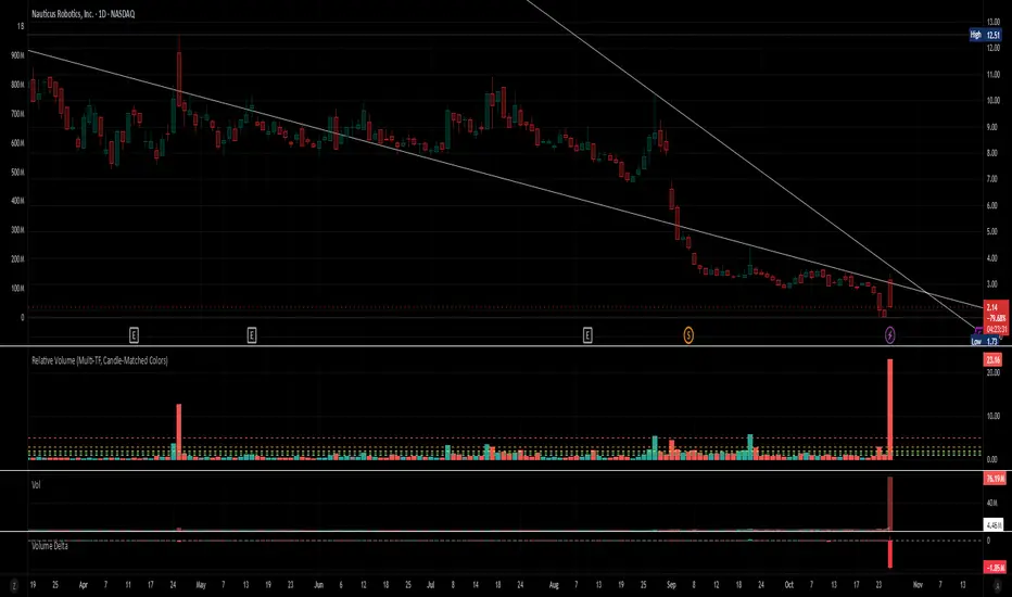
Relative Volume (Multi-TF, D, W, M)Relative Volume (Multi-TF, Candle-Matched Colors)
This indicator measures Relative Volume (RVOL) — the ratio of current volume to average historical volume — across any higher timeframe (Daily, Weekly, or Monthly) and displays it as color-coded columns that match the candle colors of the chart you’re viewing.
RVOL reveals how active today’s market participation is compared to its typical rhythm.
RVOL = 1.0 → normal volume
>1.5 → rising interest
>2.0–3.0 → strong institutional participation
>5.0 → climax or exhaustion levels
Features
Works on any chart timeframe while computing RVOL from your chosen higher timeframe (e.g., show Daily RVOL while trading on a 5-minute chart).
Column colors automatically match your chart’s candle colors (green/red/neutral).
Adjustable lookback period (len) and selectable source timeframe (D, W, or M).
Pre-drawn horizontal guide levels at 1.0, 1.2, 1.5, 2, 3, and 5 for quick interpretation.
Compatible with all chart types, including Heikin Ashi or custom color schemes.
Typical Use
Swing trading:
Look for quiet bases where RVOL stays 0.4–0.9, then expansion ≥2 on breakout days.
Confirm follow-through when green days keep RVOL ≥1.2–1.5 and red pullbacks stay below 1.0.
Day trading:
Watch intraday RVOL (on 1–5m charts) for bursts ≥2 that sustain for several bars — this signals crowd engagement and valid momentum.
Interpretation Summary
RVOL Value Meaning Typical Action
0.4–0.9 Quiet base / low interest Watch for setup
1.0 Normal activity Neutral
1.2–1.5 Valid participation Early confirmation
2–3 Strong expansion Momentum / breakout
≥5 Climax / exhaustion Take profits or avoid new entries
Author’s note:
RVOL isn’t directional; it tells how many players are active, not who’s winning. Combine it with structure (levels, VWAP, or trend) to see when the market crowd truly commits.
Curvature Tensor Pivots🌀 Curvature Tensor Pivots
Curvature Tensor Pivots: Geometric Pivot Detection Through Differential Geometry
Curvature Tensor Pivots applies mathematical differential geometry to market price analysis, identifying pivots by measuring how price trajectories bend through space. Unlike traditional pivot indicators that rely solely on price highs and lows, this system calculates the actual geometric curvature of price paths and detects inflection points where the curvature changes sign or magnitude—the mathematical hallmarks of directional transitions.
The indicator combines three components: precise curvature measurement using second-derivative calculus, tensor weighting that multiplies curvature by volatility and momentum, and a tension-based prediction system that identifies compression before pivots form. This creates a forward-looking pivot detector with built-in confirmation mechanics.
What Makes This Original
Pure Mathematical Foundation
This indicator implements the classical differential geometry curvature formula κ = |y''| / (1 + y'²)^(3/2), which measures how sharply a curve bends at any given point. In price analysis, high curvature indicates sharp directional changes (active pivots), while curvature approaching zero indicates straight-line motion (inflection points forming). This mathematical approach is fundamentally different from pattern recognition or statistical pivots—it measures the actual geometry of price movement.
Tensor Weighting System
The core innovation is the tensor scoring mechanism, which multiplies geometric curvature by two market-state variables: volatility (ATR expansion/compression) and momentum (rate of change strength). This creates a multi-dimensional strength metric that distinguishes between meaningful pivots and noise. A high tensor score means high curvature is occurring during significant volatility with strong momentum—a genuine structural turning point. Low tensor scores during high curvature indicate choppy, low-conviction moves.
Tension-Based Prediction
The system calculates tension as the inverse of curvature (Tension = 1 - κ). When curvature is low, tension is high, indicating price is moving in a straight line and approaching an inflection point where it must curve. The tension cloud visualizes this compression, tightening before pivots form and expanding after they complete. This provides anticipatory signals rather than purely reactive confirmation.
Integrated Confirmation Architecture
Rather than simply flagging high curvature, the system requires convergence of four elements: geometric inflection detection (sign changes in second derivative or curvature extrema), traditional price structure pivots (pivot highs/lows), tensor strength above threshold, and minimum spacing between signals. This multi-layer confirmation prevents false signals while maintaining sensitivity to genuine turning points.
This is not a combination of existing indicators—it's an application of pure mathematical concepts (differential calculus and tensor algebra) to market geometry, creating a unique analytical framework.
Core Components and How They Work Together
1. Differential Geometry Engine
The foundation is calculus-based trajectory analysis. The system treats price as a function y(t) and calculates:
First derivative (y'): The slope of the price trajectory, representing directional velocity
Second derivative (y''): The acceleration of slope change, representing how quickly direction is shifting
Curvature (κ): The normalized geometric bend, calculated using the formula κ = |y''| / (1 + y'²)^(3/2)
This curvature value is then normalized to a 0-1 range using adaptive statistical bounds (mean ± 2 standard deviations over a rolling window). High κ values indicate sharp bends (active pivots), while κ approaching zero indicates inflection points where the trajectory is straightening before changing concavity.
2. Tensor Weighting Components
The raw curvature is weighted by market dynamics to create the tensor score:
Volatility Component: Calculated as current ATR divided by baseline ATR (smoothed average). Values above 1.0 indicate expansion (higher conviction moves), while values below 1.0 indicate compression (lower reliability). This ensures pivots forming during volatile periods receive higher scores than those in quiet conditions.
Momentum Component: Measured using rate of change (ROC) strength normalized by recent average. High momentum indicates sustained directional pressure, confirming that curvature changes represent genuine trend shifts rather than noise.
Tensor Score Fusion: The final tensor score = κ × Volatility × Momentum × Direction × Gain. This creates a directional strength metric ranging from -1 (strong bearish curvature) to +1 (strong bullish curvature). The magnitude represents conviction, while the sign represents direction.
These components work together by filtering geometric signals through market-state context. A high curvature reading during low volatility and weak momentum produces a low tensor score (likely noise), while the same curvature during expansion and strong momentum produces a high tensor score (likely genuine pivot).
3. Inflection Point Detection System
Inflection points occur where the second derivative changes sign (concave to convex or vice versa) or where curvature reaches local extrema. The system detects these through multiple methods:
Sign change detection: When y'' crosses zero, the price trajectory is transitioning from curving upward to downward (or vice versa)
Curvature extrema: When κ reaches a local maximum or minimum, indicating peak bend intensity
Near-zero curvature: When κ falls below an adaptive threshold, indicating straight-line motion before a directional change
These geometric signals are combined with traditional pivot detection (pivot highs and lows using configurable lookback/lookahead periods) to create confirmed inflection zones. The geometric math identifies WHERE inflections are forming, while price structure confirms WHEN they've completed.
4. Tension Cloud Prediction
Tension is calculated as 1 - κ, creating an inverse relationship where low curvature produces high tension. This represents the "straightness" of price trajectory—when price moves in a straight line, it's building tension that must eventually release through a curved pivot.
The tension cloud width adapts to this tension value: it tightens (narrows) when curvature is low and tension is high, providing visual warning that a pivot is forming. After the pivot completes and curvature increases, tension drops and the cloud expands, confirming the turn.
This creates a leading indicator component within the system: watch for the cloud to compress, then wait for the pivot marker and tensor direction confirmation to enter trades.
5. Multi-Layer Visualization System
The visual components work hierarchically:
Curvature ribbons (foundation): Width expands with curvature magnitude, color shifts with tensor direction (green bullish, red bearish)
Tension cloud (prediction): Purple overlay that compresses before pivots and expands after
Tensor waves (context): Harmonic oscillating layers driven by three phase accumulators (curvature, tensor magnitude, volatility), creating visual texture that becomes erratic before pivots and smooth during trends
Inflection zones (timing): Golden background highlighting when geometric conditions indicate inflection points forming
Pivot markers (confirmation): Triangles marking confirmed pivots where geometric inflection + price structure + tensor strength all align
Each layer adds information without redundancy: ribbons show current state, tension shows prediction, waves show regime character, zones show geometric timing, and markers show confirmed entries.
Calculation Methodology
Phase 1 - Derivative Calculations
Price is normalized by dividing by a 50-period moving average to improve numerical stability. The first derivative is calculated as the bar-to-bar change, then smoothed using a configurable smoothing length (default 3 bars) to reduce noise while preserving structure.
The second derivative is calculated as the bar-to-bar change in the first derivative, also smoothed. This represents the acceleration of directional change—positive values indicate price is curving upward (concave up), negative values indicate curving downward (concave down).
Phase 2 - Curvature Formula
The classical curvature formula is applied:
Calculate y'² (first derivative squared)
Calculate (1 + y'²)^1.5 as the denominator
Divide |y''| by this denominator to get raw curvature κ
This formula ensures curvature is properly normalized regardless of the steepness of the trajectory. A vertical line with high slope (large y') can still have low curvature (straight), while a gradual slope with changing direction produces high curvature (curved).
The raw curvature is then normalized to 0-1 range using adaptive bounds (rolling mean ± 2 standard deviations), allowing the system to adapt to different market volatility regimes.
Phase 3 - Tensor Weighting
ATR is calculated over the specified volatility length (default 14). Current ATR is divided by smoothed ATR to create the volatility ratio. Momentum is calculated as the rate of change over the momentum length (default 10), normalized by recent average ROC.
The tensor score is computed as: Curvature × Volatility × Momentum × Tensor Gain × Direction Sign
This creates the final directional strength metric used for ribbon coloring and signal generation.
Phase 4 - Inflection Detection
Multiple conditions are evaluated simultaneously:
Second derivative sign changes (y'' × y'' < 0)
Curvature local maxima (previous bar κ > current bar κ AND previous bar κ > two bars ago κ)
Curvature local minima (opposite condition)
Low curvature threshold (current κ < adaptive threshold)
Any of these conditions triggers inflection zone highlighting. For confirmed pivot signals, inflection detection must coincide with traditional pivot highs/lows AND tensor magnitude must exceed threshold AND minimum spacing since last signal must be satisfied.
Phase 5 - Tension Calculation
Tension = 1 - κ (smoothed)
This inverse relationship creates the compression/expansion dynamic. When curvature approaches zero (straight trajectory), tension approaches 1 (maximum compression). When curvature is high (sharp bend), tension approaches zero (released).
The tension cloud bands are calculated as: Basis ± (Ribbon Width × Tension)
This creates the visual tightening effect before pivots.
Phase 6 - Wave Generation
Three phase accumulators are maintained:
Phase 1: Accumulates based on curvature magnitude (0.1 × κ per bar)
Phase 2: Accumulates based on tensor magnitude (0.15 × tensor per bar)
Phase 3: Accumulates based on volatility (0.08 × volatility per bar)
For each wave layer (2-8 configurable), a unique frequency is used (layer number × 0.6). The wave offset is calculated as:
Amplitude × (sin(phase1 × frequency) × 0.4 + sin(phase2 × frequency × 1.2) × 0.35 + sin(phase3 × frequency × 0.8) × 0.25)
This creates complex harmonic motion that reflects the interplay of curvature, strength, and volatility. When these components are aligned, waves are smooth; when misaligned (pre-pivot conditions), waves become chaotic.
All calculations are deterministic and execute on closed bars only—there is no repainting.
How to Use This Indicator
Setup and Configuration
Apply the indicator to your chart with default settings initially
Enable the main dashboard (top right recommended) to monitor curvature, tensor, and tension metrics in real-time
Enable the curvature matrix (bottom right) to see historical patterns in the heatmap
Choose your ribbon mode: "Dual Ribbon" shows both bullish and bearish zones, "Tension Cloud" emphasizes the compression zones
For your first session, observe how the tension cloud behaves before confirmed pivots—you'll notice it consistently tightens (narrows) before pivot markers appear, then expands after.
Signal Interpretation
High Pivot (Bearish) - Red triangle above price:
Occurs when price makes a pivot high (local maximum)
Second derivative is negative (concave down curvature)
Tensor magnitude exceeds threshold (strong confirmation)
Minimum spacing requirement met (noise filter)
Interpretation: A confirmed bearish inflection point has formed. Price trajectory has curved over and is transitioning from upward to downward movement.
Low Pivot (Bullish) - Blue triangle below price:
Occurs when price makes a pivot low (local minimum)
Second derivative is positive (concave up curvature)
Tensor magnitude exceeds threshold
Spacing requirement met
Interpretation: A confirmed bullish inflection point has formed. Price trajectory has curved upward and is transitioning from downward to upward movement.
Dashboard Metrics
κ (Curvature): 0-100% reading. Above 70% = sharp active pivot, 40-70% = moderate curve, below 40% = gentle or approaching inflection
Tensor: Directional strength. Arrow indicates bias (⬆ bullish, ⬇ bearish, ⬌ neutral). Magnitude indicates conviction.
Volatility: Current ATR expansion state. Above 70% = high volatility (pivots more significant), below 40% = compressed (pivots less reliable)
Momentum: Directional strength. High values confirm trend continuation, low values suggest exhaustion
Tension: 0-100% reading. Above 70% = pivot forming soon (high compression), below 40% = pivot recently completed (expanded)
State: Real-time regime classification:
"🟢 STABLE" = normal trending conditions
"🟡 TENSION" = pivot forming (high compression)
"🔴 HIGH κ" = active sharp pivot in progress
"⚠ INFLECTION" = geometric inflection zone (critical transition)
Curvature Matrix Heatmap
The matrix shows the last 30 bars (configurable 10-100) of historical data across five metrics:
κ row: Curvature evolution (green = low, yellow = moderate, red = high)
Tension row: Purple intensity shows compression building
Tensor row: Strength evolution (green = strong, yellow = moderate, red = weak)
Volatility row: Expansion state
Momentum row: Directional conviction
Pattern recognition: Look for purple clustering in the tension row followed by red spikes in the κ row—this shows compression → release pivot sequence.
Trading Workflow
Step 1 - Monitor Tension:
Watch the tension cloud and dashboard tension metric. When tension rises above 60-70% and the cloud visibly tightens, a pivot is building. The matrix will show purple bands clustering.
Step 2 - Identify Inflection Zone:
Wait for the golden background glow (inflection zone) to appear. This indicates the geometric conditions are met: curvature is approaching zero, second derivative is near sign change, or curvature extrema detected. The dashboard state will show "⚠ INFLECTION ZONE".
Step 3 - Confirm Direction:
Check the tensor arrow in the dashboard:
⬆ (bullish tensor) = expect bullish pivot
⬇ (bearish tensor) = expect bearish pivot
Also verify the y'' status in the dashboard:
"🔵↑ Concave Up" = bullish curvature forming
"🔴↓ Concave Down" = bearish curvature forming
Step 4 - Wait for Pivot Marker:
Do not enter on inflection zones alone—wait for the confirmed pivot marker (triangle). This ensures all confirmation layers have aligned: geometric inflection + price structure pivot + tensor strength + spacing filter.
Step 5 - Execute Entry:
Long entry: Blue triangle below price + ⬆ tensor + tension releasing (dropping)
Short entry: Red triangle above price + ⬇ tensor + tension releasing
Step 6 - Manage Risk:
Initial stop: Place beyond the opposite ribbon edge plus one ATR buffer
Trailing stop: Follow the ribbon edge (basis ± adaptive width) as curvature sustains in your direction
Exit signal: If tension spikes again quickly (another inflection forming), consider taking profit—the trend may be reversing
Best Practices
Use multiple timeframe confirmation: Check that higher timeframe tensor aligns with your trade direction
Respect the spacing filter: If a pivot just fired, wait for minimum spacing before taking another signal
Distinguish regime: In "🔴 HIGH κ" state (choppy), reduce position size; in "🟢 STABLE" state, full confidence
Combine with support/resistance: Pivots near key levels have higher probability
Watch particle density: Clustering of particles indicates rising curvature intensity
Observe wave texture: Smooth flowing waves = trending environment (pivots are reversals); chaotic erratic waves = reversal environment (pivots are trend starts)
Ideal Market Conditions
Best Performance
Liquid markets with clear swing structure (forex majors, large-cap stocks, major indices)
Timeframes from 15-minute to daily (the system adapts across timeframes)
Markets with periodic swings and clear directional phases (where geometric curvature is meaningful)
Trending markets with consolidation phases (where tension builds before breakouts)
Challenging Conditions
Extremely choppy/sideways markets for extended periods (high curvature but low tensor magnitude—system will reduce signals appropriately)
Very low liquidity instruments (erratic price action creates false geometric signals)
Ultra-low timeframes (1-minute or below) where spread and noise dominate structure
Markets in deep consolidation (the system will show high tension but no clean pivot confirmation)
The indicator is designed to adapt: in poor conditions, tensor scores remain low and signals reduce naturally. In optimal conditions, tension compression → inflection → pivot confirmation sequences occur cleanly.
Parameter Optimization by Trading Style
Scalping (5-15 Minute Charts)
Curvature Window: 3-5 (faster response)
Curvature Smoothing: 2 (minimal lag)
Volatility Length: 10-14
Momentum Length: 8-10
Tensor Gain: 1.2-1.5 (moderate sensitivity)
Inflection Threshold: 0.10-0.15 (more sensitive)
Min Pivot Spacing: 3-5 bars
Pivot Mode: Aggressive
Ribbon Mode: Dual Ribbon (clearer entries)
Day Trading (15-60 Minute Charts)
Curvature Window: 5 (default)
Curvature Smoothing: 3 (balanced)
Volatility Length: 14
Momentum Length: 10
Tensor Gain: 1.5 (default)
Inflection Threshold: 0.15 (default)
Min Pivot Spacing: 5-8 bars
Pivot Mode: Normal or Adaptive
Ribbon Mode: Dual Ribbon
Swing Trading (4-Hour to Daily Charts)
Curvature Window: 7-10 (smoother)
Curvature Smoothing: 4-5 (noise reduction)
Volatility Length: 20-30
Momentum Length: 14-20
Tensor Gain: 1.8-2.5 (higher conviction requirement)
Inflection Threshold: 0.20-0.30 (more selective)
Min Pivot Spacing: 8-12 bars
Pivot Mode: Conservative
Ribbon Mode: Tension Cloud (focus on compression zones)
Performance Optimization
If you experience lag on lower-end systems:
Reduce Wave Layers: 4 → 2 (50% reduction in calculations)
Lower Particle Density: 3 → 1 (66% reduction in label creation)
Decrease Matrix History: 30 → 15 bars (50% reduction in table size)
Disable Tensor Waves entirely if not needed for your trading
Important Disclaimers
- This indicator is a technical analysis tool designed to identify potential pivot points through mathematical analysis of price trajectory geometry. It should not be used as a standalone trading system. Always combine with proper risk management, position sizing, and additional confirmation methods (support/resistance, volume analysis, multi-timeframe alignment).
- The curvature and tensor calculations are deterministic mathematical formulas applied to historical price data—they do not predict future price movements with certainty. Past geometric patterns do not guarantee future pivot behavior. The tension-based prediction system identifies conditions where pivots are likely to form based on trajectory straightness, but market conditions can change rapidly.
- All trading involves risk. Use appropriate stop losses and never risk more than you can afford to lose. The signal spacing filters and tensor confirmation layers are designed to reduce noise, but no indicator can eliminate false signals entirely.
This system is most effective when combined with sound trading principles, market context awareness, and disciplined execution.
Technical Notes
All calculations execute on closed bars only (no repainting)
Lookback functions limited to 5000 bars maximum
Arrays are fixed-size (waves) or hard-capped (particles at 80 labels)
Dashboard and matrix update only on the last bar to minimize computational load
Particle generation throttled to every 2 bars
Phase accumulators use modulo operations to prevent overflow
Statistical normalization (mean ± 2σ) automatically adapts to different volatility regimes
— Dskyz, Trade with insight. Trade with anticipation.
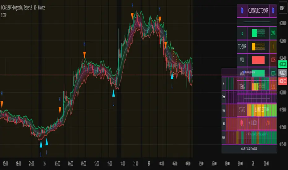
Multi-Timeframe Granville Signal──────────────────────────────────────────
OVERVIEW
──────────────────────────────────────────
MTF Granville Signal is an invite-only Pine Script indicator that assists traders in identifying high-probability entry points based on Granville's Law principles, enhanced with Multi-Timeframe (MTF) structural analysis and dynamic Moving Average Deviation Rate (MADR) filtering.
This indicator is NOT investment advice. It is a technical analysis tool. All trading decisions and outcomes are the sole responsibility of the user.
──────────────────────────────────────────
WHAT MAKES THIS INDICATOR ORIGINAL
──────────────────────────────────────────
While many indicators implement basic Granville's Law or simple moving average crosses, this indicator distinguishes itself through two mathematically rigorous enhancements:
1. Dynamic MADR Filtering with Statistical Foundation
Unlike fixed percentage bands used in conventional overbought/oversold indicators, this system employs adaptive threshold calculation based on rolling standard deviation :
Mathematical Approach:
Calculates price deviation from the reference Simple Moving Average(SMA) as a percentage
Computes standard deviation (σ) over an extended lookback period
Default: 1σ threshold = 68.26% probability zone under normal distribution
User-configurable sigma multiplier (1σ, 2σ, 3σ)
Operational Logic:
Trend-following signals (Granville Rules 1, 2, 3, 5, 6, 7) : Fire only when MADR is within normal range (< threshold), indicating healthy trend conditions
Counter-trend signals (Granville Rules 4, 8) : Fire only when MADR exceeds threshold, indicating statistical over-extension and mean-reversion probability
Why This Matters:
Traditional indicators use arbitrary fixed thresholds (e.g., "overbought above +3%"). Market volatility varies dramatically across assets and time periods. A 3% deviation in EUR/USD may be extreme, while in Bitcoin it's noise. Dynamic MADR automatically adapts to each market's volatility characteristics, maintaining consistent statistical validity across diverse trading instruments.
2. MTF Structural Verification for Cycle-Phase Filtering
This is not merely displaying multiple timeframe SMAs on a chart. The indicator performs structural analysis to determine trend cycle phase :
Verification Mechanism:
Checks if price has recently touched/crossed the higher timeframe SMA within a configurable lookback period
Confirms SMA hierarchy alignment (short-term > mid-term > long-term for uptrends)
Distinguishes between early-cycle trend initiation and late-cycle exhaustion
Why This Matters:
Granville's Law signals can appear throughout a trend cycle, but probability varies significantly:
Early cycle (price recently interacted with higher TF SMA): High probability - catching trend initiation or deep retracements
Late cycle (price extended far from higher TF SMA): Low probability - entering during exhaustion phase
By requiring recent structural interaction with higher timeframe SMAs, the indicator filters out low-probability late-cycle entries, dramatically improving signal quality.
──────────────────────────────────────────
GRANVILLE'S LAW IMPLEMENTATION
──────────────────────────────────────────
This indicator implements all eight of Joseph Granville's classic rules, with a focus on Rules 1, 2, 3,4, 5, 6, 7, and 8 for primary signal generation. Rules 3 and 7 are operationalized through touch-based approximation (see explanation below):
Trend-Following Signals (Rules 1, 2, 3, 5, 6, 7)
Buy Signals:
Short-term SMA crosses above (or touches and bounces off) mid/long-term SMAs
SMA hierarchy confirms uptrend structure
MADR indicates price is NOT over-extended
Price recently interacted with higher timeframe SMA (MTF verification)
Sell Signals:
Mirror logic for downtrends
Counter-Trend Mean-Reversion Signals (Rules 4, 8)
Sell Signals:
Price shows extreme deviation from reference SMA (MADR exceeds threshold)
Price begins reverting toward SMA
Short-term SMA crosses below (or touches and bounces off) mid/long-term SMAs
Recent structural interaction with higher timeframe SMA confirms reversal setup
Buy Signals:
Mirror logic for oversold reversals
How Rules 3 and 7 Are Handled:
Rules 3 and 7 describe "price approaches the SMA." Rather than excluding these rules, this indicator approximates "approaches" as "touches the SMA" to eliminate ambiguity. In practice, defining "approaches" is subjective and adds complexity. By operationalizing "approaches" as "touches/crosses," the indicator maintains mechanical objectivity while still capturing the intent of Rules 3 and 7.
──────────────────────────────────────────
WHY GRANVILLE'S LAW?
──────────────────────────────────────────
Universality: Functions across all markets (forex, stocks, crypto, commodities) and timeframes
Simplicity: Based solely on price-to-moving-average relationships—no complex calculations
Reproducibility: Mechanical rules eliminate emotional bias
60+ Year Track Record: Proven principle since Joseph Granville's 1960 publication
──────────────────────────────────────────
TECHNICAL ARCHITECTURE
──────────────────────────────────────────
Signal Generation Process
Calculate SMAs across multiple timeframes (short/mid/long-term periods)
Compute MADR : Measure price deviation from reference SMA and its statistical significance
Verify MTF Structure : Check recent price interaction with higher timeframe SMA
Evaluate SMA Hierarchy : Confirm trend direction via SMA alignment
Apply Granville Logic : Detect specific Rule patterns (crosses, touches, bounces)
Determining deviation from SMA :
• Trend-following: MADR < threshold (healthy trend)
• Counter-trend: MADR > threshold (over-extension)
Signal Interval Control : Cooldown period prevents alert spam during noise
Why This Combination Works
The synthesis of these three components creates a robust filtering system:
Granville's Law provides the fundamental signal logic (proven over decades)
Dynamic MADR prevents entries at dangerous price extremes (volatility-adaptive risk management)
MTF Structural Verification ensures signals occur at optimal cycle phases (timing optimization)
No single element alone produces high-quality signals. Their integration may generate edge in trending market conditions.
──────────────────────────────────────────
WHAT THIS INDICATOR DOES NOT DO
──────────────────────────────────────────
To set realistic expectations:
❌ Does not predict future price direction with certainty
❌ Does not guarantee profitable trades
❌ Does not work equally well in all market conditions (see below for limitations)
❌ Does not replace risk management, position sizing, or trading discipline
❌ Does not provide trade exit signals (focus is on entry timing)
──────────────────────────────────────────
PARAMETER CONFIGURATION
──────────────────────────────────────────
Mid Term Trend Check Enabled (Default: true)
Activates SMA hierarchy verification for mid-term trend confirmation.
When enabled: Signals require short-term SMA > mid-term SMA (uptrend) or vice versa (downtrend)
When disabled: Only short-term SMA behavior is evaluated
Recommendation : Keep enabled for most use cases to filter weak trends
Long Term Trend Check Enabled (Default: true)
Adds long-term SMA to hierarchy verification for additional trend strength confirmation.
Requires Mid Term Trend Check to be enabled
When enabled: Signals require short-term SMA > mid-term SMA > long-term SMA alignment
Recommendation : Enable on lower timeframes (15m or below) for stronger filtering. Disable on higher timeframes (1h or above) as the additional filter becomes redundant and overly restrictive
Require Touch Higher Timeframe SMA Enabled (Default: true)
Enforces recent price interaction with higher timeframe SMA to filter late-cycle entries.
When enabled: Signals fire only if price touched/crossed mid-term or long-term SMA within lookback period
When disabled: Signals can fire regardless of recent SMA interaction (more signals, lower quality)
Recommendation : Keep enabled. This is a core filter for cycle-phase discrimination
Touch Higher Timeframe SMA Lookback Period (Default: 24 bars)
Defines how far back to search for price-SMA interaction.
Lower values (12-18): Stricter filtering, fewer signals, earlier cycle detection
Higher values (24-36): More lenient filtering, more signals, includes some mid-cycle entries
Recommendation : Adjust based on market volatility. Trending markets: use lower values. Choppy markets: use higher values to capture valid retracements
SMA Short Term Period (Default: 20)
Primary SMA for Granville's Law pattern detection.
Lower values (10-15): More responsive, more signals, higher noise
Higher values (25-40): Smoother, fewer signals, delayed entries
Recommendation : 20 is standard across most markets. Adjust ±5 based on your timeframe preference
SMA Mid Term Period (Default: 80)
Reference SMA for trend hierarchy and MTF verification.
Typically 3-5x the short-term period
Recommendation : 80 works well for intraday (15m, 1h) and swing trading (4h, daily). Maintain ratio relationship with short-term SMA
SMA Long Term Period (Default: 320)
Optional trend strength filter (requires Long Term Trend Check enabled).
Typically 4x the mid-term period
Recommendation : 320 is appropriate for multi-day trend analysis. Not critical for intraday scalping
SMA Period for Divergence (Default: 1920)
Lookback period for calculating MADR standard deviation. Two approaches:
Approach 1: Chart Timeframe SMA (Simple)
Use 20 periods matching your chart timeframe for straightforward deviation measurement.
Example: 20 periods on any timeframe
Approach 2: Higher Timeframe SMA (MTF Analysis)
Use period equivalent to higher timeframe's 20-period SMA for multi-timeframe structural analysis.
Recommendation for day trading :
• 15m chart: 1920 periods (≈ daily 20-SMA: 20 days × 96 bars/day)
• 1h chart: 480 periods (≈ daily 20-SMA: 20 days × 24 bars/day)
• 4h chart: 120 periods (≈ daily 20-SMA: 20 days × 6 bars/day)
Both approaches are valid. Approach 2 incorporates higher timeframe context into MADR filtering.
MADR Standard Deviation Band (Sigma) (Default: 1.00)
Statistical threshold for determining trend overheating vs. healthy conditions.
1.0σ = 68.26% probability zone (default, balanced)
2.0σ = 95.44% probability zone (stricter, fewer counter-trend signals)
3.0σ = 99.74% probability zone (very strict, rare extreme reversals only)
Recommendation : Start with 1.0σ. Increase to 2.0σ if you want to trade only extreme mean-reversion opportunities. Decrease to 0.5σ-0.8σ for more aggressive trend-following
Signal Minimum Interval (Default: 4 hours)
Cooldown period between signals to prevent alert spam during consolidation.
Measured in hours regardless of chart timeframe
0 = no cooldown (all valid signals fire)
2-4 = typical for day trading
8-12 = typical for swing trading
Recommendation : Match to your trading frequency. Day traders: 2-4 hours. Swing traders: 8-12 hours
Buy/Sell Signal Text Color (Default: Blue)
Reversal Buy/Sell Signal Text Color (Default: Purple)
Customize label colors for visual distinction between trend-following and counter-trend signals.
Alert Display Prefix (Default: Auto-detected from chart timeframe)
Prefix for alert messages (e.g., "1h", "15m"). Auto-filled if left blank.
──────────────────────────────────────────
RECOMMENDED CONFIGURATIONS
──────────────────────────────────────────
Configuration 1: Aggressive Day Trading (15m Chart)
SMA Short: 20
SMA Mid: 80
SMA Long: 320
MADR SMA Period: 1920
MADR Sigma: 1.0
Signal Interval: 4 hours
Touch Lookback: 24 bars
Long Term Trend Check: Enabled
Use case: Active day trading, multiple signals per session
Configuration 2: Balanced Day Trading (1h Chart)
SMA Short: 20
SMA Mid: 80
MADR SMA Period: 480
MADR Sigma: 1.0
Signal Interval: 4 hours
Touch Lookback: 24 bars
Long Term Trend Check: Disabled
Use case: Standard day trading, moderate signal frequency
──────────────────────────────────────────
TECHNICAL LIMITATIONS AND UNSUITABLE CONDITIONS
──────────────────────────────────────────
This indicator has known limitations:
1. Range/Choppy Markets
Extended consolidation generates false signals and whipsaw entries. Wait for clear breakout or use higher timeframe trend filters.
2. Low Liquidity Instruments
In exotic pairs, microcap stocks, or illiquid assets, wide spreads and slippage erode edge. Stick to major high-volume instruments.
3. News-Driven Volatility
Fundamental shocks invalidate technical patterns. Avoid trading around scheduled high-impact news events.
4. Algorithmic Regime Changes
Market microstructure evolves over time. Review performance periodically and adjust parameters if edge deteriorates.
5. Extreme Market Regimes
Black swan events and unprecedented volatility cause all technical systems to fail simultaneously. Use circuit breakers and position size limits.
6. Gap Openings
Price gaps over weekends or between sessions invalidate some signals. Reduce position sizing accordingly.
──────────────────────────────────────────
OPEN-SOURCE CODE TRANSPARENCY
──────────────────────────────────────────
While the source code is proprietary and protected, the fundamentals are fully explainable:
SMA calculation : Standard Pine Script ta.sma() function
MADR calculation : (close - sma) / sma * 100 and ta.stdev() for threshold
MTF data retrieval : request.security() for higher timeframe values
Granville pattern detection : Logical comparison of price/SMA positions and crosses
No "black box" algorithms. No hidden magic. Only rigorous application of proven technical principles.
──────────────────────────────────────────
OPEN-SOURCE CODE REUSE
──────────────────────────────────────────
This indicator does NOT reuse code from other TradingView scripts. All logic is proprietary.
Standard Pine Script functions (ta.sma, ta.stdev, request.security, etc.) used per documented API
No third-party libraries or external dependencies
No license conflicts
──────────────────────────────────────────
VERSION INFORMATION
──────────────────────────────────────────
Current Version : 6 (Pine Script v6)
Author : © 2025 mmntmr369. All rights reserved.
Publication Type : Invite-only (Proprietary source code)
──────────────────────────────────────────
DISCLAIMER : This indicator is provided for educational and informational purposes only. It does not constitute investment advice, financial advice, trading advice, or any other type of advice. You should not make any investment decisions based solely on this indicator. Always conduct your own research and consult with a licensed financial professional before making investment decisions. Past performance does not indicate future results. Trading carries substantial risk of loss and is not suitable for all investors.
══════════════════════════════════════════
日本語版 / JAPANESE VERSION
══════════════════════════════════════════
──────────────────────────────────────────
概要
──────────────────────────────────────────
MTF Granville Signalは、グランビルの法則の原則に基づいた高確率エントリーポイントの特定を支援する招待制Pine Scriptインジケーターです。マルチタイムフレーム(MTF)構造分析と動的移動平均線乖離率(MADR)フィルタリングにより強化されています。
本インジケーターは投資助言ではありません。 これはテクニカル分析ツールです。すべての取引判断と結果は、ユーザーの単独責任となります。
──────────────────────────────────────────
本インジケーターの独自性
──────────────────────────────────────────
多くのインジケーターが基本的なグランビルの法則または単純な移動平均クロスを実装していますが、本インジケーターは2つの数学的に厳密な拡張機能によって差別化されます:
1. 統計的基盤を持つ動的MADRフィルタリング
従来の買われ過ぎ/売られ過ぎインジケーターで使用される固定パーセンテージバンドとは異なり、本システムは ローリング標準偏差に基づく適応的閾値計算 を採用しています:
数学的アプローチ:
参照SMAからの価格偏差をパーセンテージとして計算
拡張ルックバック期間にわたって標準偏差(σ)を計算
デフォルト:1σ閾値 = 正規分布下の68.26%確率ゾーン
ユーザー設定可能なシグマ乗数(1σ、2σ、3σ)
操作ロジック:
順張りシグナル(グランビル法則1、2、3、5、6、7) :MADRが正常範囲内(<閾値)にある場合のみ発火し、健全なトレンド状態を示します
逆張りシグナル(グランビル法則4、8) :MADRが閾値を超える場合のみ発火し、統計的過度の拡張と平均回帰確率を示します
重要な理由:
従来のインジケーターは任意の固定閾値(例:「+3%以上で買われ過ぎ」)を使用します。市場のボラティリティは資産と期間によって劇的に変化します。EUR/USDでの3%偏差は極端かもしれませんが、ビットコインではノイズです。動的MADRは各市場のボラティリティ特性に自動的に適応し、多様な取引商品全体で一貫した統計的妥当性を維持します。
2. サイクルフェーズフィルタリングのためのMTF構造検証
これは単にチャート上に複数の時間足SMAを表示するだけではありません。インジケーターは トレンドサイクルフェーズを決定するための構造分析 を実行します:
検証メカニズム:
設定可能なルックバック期間内に価格が上位時間足SMAに最近タッチ/クロスしたかどうかを確認
SMA階層の整列を確認(上昇トレンドでは短期>中期>長期)
初期サイクルトレンド開始と後期サイクル疲弊を区別
重要な理由:
グランビルの法則シグナルはトレンドサイクル全体で出現できますが、確率は大きく異なります:
初期サイクル (価格が最近上位TF SMAと相互作用):高確率 - トレンド開始または深い調整を捕捉
後期サイクル (価格が上位TF SMAから遠く離れている):低確率 - 疲弊フェーズ中のエントリー
上位時間足SMAとの最近の構造的相互作用を要求することで、インジケーターは低確率の後期サイクルエントリーを除外し、シグナル品質を劇的に向上させます。
──────────────────────────────────────────
グランビルの法則実装
──────────────────────────────────────────
本インジケーターはジョセフ・グランビルの古典的な8つの法則すべてを実装しており、 法則1、2、3、4、5、6、7、8 に焦点を当てた主要シグナル生成を行います。法則3と7はタッチベースの近似で運用されます(以下の説明を参照):
順張りシグナル(法則1、2、3、5、6、7)
買いシグナル:
短期SMAが中期/長期SMAを上回って交差する(またはタッチしてバウンス)
SMA階層が上昇トレンド構造を確認
MADRが価格が過度に拡張されていないことを示す
価格が最近上位時間足SMAと相互作用した(MTF検証)
売りシグナル:
下降トレンドの場合は反対のロジック
逆張り平均回帰シグナル(法則4、8)
売りシグナル:
価格が参照SMAから極端に乖離(MADRが閾値を超える)
価格がSMAに向かって反転を開始
短期SMAが中期/長期SMAを下回って交差する(またはタッチしてバウンス)
上位時間足SMAとの最近の構造的相互作用が反転セットアップを確認
買いシグナル:
売られ過ぎ反転の場合は反対のロジック
法則3と7の取り扱い:
法則3と7は「価格がSMAに接近する」と説明しています。これらの法則を除外するのではなく、本インジケーターは曖昧さを排除するために「接近」を「SMAにタッチ」として近似します。実際には、「接近」の定義は主観的で複雑さを追加します。「接近」を「タッチ/クロス」として運用することで、インジケーターは法則3と7の意図を捕捉しながら機械的客観性を維持します。
──────────────────────────────────────────
なぜグランビルの法則?
──────────────────────────────────────────
普遍性: すべての市場(外国為替、株式、暗号、商品)および時間足で機能
シンプルさ: 価格対移動平均の関係のみに基づく - 複雑な計算なし
再現性: 機械的ルールが感情的バイアスを排除
60年以上の実績: ジョセフ・グランビルの1960年の出版以来実証された原則
──────────────────────────────────────────
技術アーキテクチャ
──────────────────────────────────────────
シグナル生成プロセス
SMAを計算 複数の時間足にわたって(短期/中期/長期期間)
MADRを計算 :参照SMAからの価格偏差とその統計的有意性を測定
MTF構造を検証 :上位時間足SMAとの最近の価格相互作用を確認
SMA階層を評価 :SMA整列によってトレンド方向を確認
グランビルロジックを適用 :特定の法則パターンを検出(クロス、タッチ、バウンス)
SMAからの乖離を判定 :
• 順張り:MADR < 閾値(健全なトレンド)
• 逆張り:MADR > 閾値(過度の拡張)
シグナル間隔制御 :クールダウン期間がノイズ中のアラートスパムを防止
なぜこの組み合わせが機能するか
これら3つのコンポーネントの統合が堅牢なフィルタリングシステムを生成します:
グランビルの法則 が基本的なシグナルロジックを提供(数十年にわたって実証)
動的MADR が危険な価格極値でのエントリーを防止(ボラティリティ適応的リスク管理)
MTF構造検証 がシグナルを最適なサイクルフェーズで発生させる(タイミング最適化)
単一の要素だけでは高品質のシグナルは生成されません。それらの統合はトレンド相場環境においてエッジを生み出す可能性があります。
──────────────────────────────────────────
本インジケーターが行わないこと
──────────────────────────────────────────
現実的な期待を設定するために:
❌ 将来の価格方向を確実に予測しない
❌ 収益性のある取引を保証しない
❌ すべての市場環境で等しく機能しない(限界については下記参照)
❌ リスク管理、ポジションサイジング、または取引規律を置き換えない
❌ 取引の手仕舞いシグナルを提供しない(焦点はエントリータイミング)
──────────────────────────────────────────
パラメータ設定
──────────────────────────────────────────
Mid Term Trend Check Enabled(中期トレンドチェック有効) (デフォルト: true)
中期トレンド確認のためのSMA階層検証を有効化。
有効時:シグナルは短期SMA > 中期SMA(上昇トレンド)またはその逆(下降トレンド)を要求
無効時:短期SMAの動作のみを評価
推奨 :弱いトレンドをフィルタリングするため、ほとんどの用途で有効を維持
Long Term Trend Check Enabled(長期トレンドチェック有効) (デフォルト: true)
追加のトレンド強度確認のため、長期SMAをSMA階層検証に追加。
中期トレンドチェックの有効化が必要
有効時:シグナルは短期SMA > 中期SMA > 長期SMAの整列を要求
推奨 :低時間足(15分足以下)でより強力なフィルタリングのため有効化。高時間足(1時間足以上)では追加フィルターが冗長かつ過度に制限的になるため無効化
Require Touch Higher Timeframe SMA Enabled(上位足SMAタッチ要求有効) (デフォルト: true)
後期サイクルエントリーをフィルタリングするため、上位時間足SMAとの最近の価格相互作用を強制。
有効時:シグナルはルックバック期間内に価格が中期または長期SMAにタッチ/クロスした場合のみ発火
無効時:最近のSMA相互作用に関係なくシグナル発火(多くのシグナル、低品質)
推奨 :有効を維持。これはサイクルフェーズ識別のコアフィルター
Touch Higher Timeframe SMA Lookback Period(上位足SMAタッチルックバック期間) (デフォルト: 24バー)
価格-SMA相互作用を検索する遡及期間を定義。
低い値(12-18):厳格なフィルタリング、少ないシグナル、初期サイクル検出
高い値(24-36):寛容なフィルタリング、多くのシグナル、中期サイクルエントリーを含む
推奨 :市場ボラティリティに基づいて調整。トレンド市場:低い値を使用。荒れた市場:有効な調整を捉えるため高い値を使用
SMA Short Term Period(SMA短期期間) (デフォルト: 20)
グランビルの法則パターン検出のための主要SMA。
低い値(10-15):反応的、多くのシグナル、高いノイズ
高い値(25-40):滑らか、少ないシグナル、遅延エントリー
推奨 :20はほとんどの市場で標準。時間足の好みに基づいて±5調整
SMA Mid Term Period(SMA中期期間) (デフォルト: 80)
トレンド階層とMTF検証のための基準SMA。
通常、短期期間の3-5倍
推奨 :80はデイトレ(15m、1h)とスイングトレード(4h、日足)に適している。短期SMAとの比率関係を維持
SMA Long Term Period(SMA長期期間) (デフォルト: 320)
オプションのトレンド強度フィルター(長期トレンドチェック有効時必要)。
通常、中期期間の4倍
推奨 :320は数日間のトレンド分析に適している。デイトレ、スイングには重要でない
SMA Period for Divergence(乖離のためのSMA期間) (デフォルト: 1920)
MADR標準偏差計算のためのルックバック期間。2つのアプローチがあります:
アプローチ1:チャート時間足SMA(シンプル)
チャート時間足と同じ20期間を使用し、シンプルに乖離を測定。
例:どの時間足でも20期間
アプローチ2:上位時間足SMA(MTF分析)
上位時間足の20期間SMA相当の期間を設定し、マルチタイムフレーム構造分析として利用。
デイトレーディング推奨設定 :
• 15分足チャート:1920期間(≈ 日足20-SMA:20日 × 96本/日)
• 1時間足チャート:480期間(≈ 日足20-SMA:20日 × 24本/日)
• 4時間足チャート:120期間(≈ 日足20-SMA:20日 × 6本/日)
両アプローチとも有効。アプローチ2は上位時間足のコンテクストをMADRフィルタリングに組み込む。
MADR Standard Deviation Band (Sigma)(MADR標準偏差バンド(シグマ)) (デフォルト: 1.00)
トレンド過熱と健全状態を判定するための統計的閾値。
1.0σ = 68.26%確率ゾーン(デフォルト、バランス型)
2.0σ = 95.44%確率ゾーン(厳格、少ない逆張りシグナル)
3.0σ = 99.74%確率ゾーン(非常に厳格、稀な極端反転のみ)
推奨 :1.0σから開始。極端な平均回帰機会のみを取引したい場合は2.0σに増加。より積極的な順張りのため0.5σ-0.8σに減少
Signal Minimum Interval(シグナル最小間隔) (デフォルト: 4時間)
保ち合い中のアラートスパムを防ぐためのシグナル間のクールダウン期間。
チャート時間足に関係なく時間で測定
0 = クールダウンなし(すべての有効なシグナルが発火)
2-4 = デイトレード取引の典型
8-12 = スイング取引の典型
推奨 :取引頻度に合わせる。デイトレーダー:2-4時間。スイングトレーダー:8-12時間
Buy/Sell Signal Text Color(買い/売りシグナルテキスト色) (デフォルト: 青)
Reversal Buy/Sell Signal Text Color(反転買い/売りシグナルテキスト色) (デフォルト: 紫)
順張りシグナルと逆張りシグナルの視覚的区別のためのラベル色をカスタマイズ。
Alert Display Prefix(アラート表示プレフィックス) (デフォルト: チャート時間足から自動検出)
アラートメッセージのプレフィックス(例:「1h」、「15m」)。空白の場合自動入力。
──────────────────────────────────────────
推奨設定例
──────────────────────────────────────────
設定1:積極的デイトレ(15分足チャート)
SMA Short: 20
SMA Mid: 80
SMA Long: 320
MADR SMA Period: 1920
MADR Sigma: 1.0
Signal Interval: 4時間
Touch Lookback: 24バー
Long Term Trend Check: 有効
用途: アクティブなデイトレード、セッションあたり複数のシグナル
設定2:バランス型デイトレ(1時間足チャート)
SMA Short: 20
SMA Mid: 80
MADR SMA Period: 480
MADR Sigma: 1.0
Signal Interval: 4時間
Touch Lookback: 24バー
Long Term Trend Check: 無効
用途: 標準的デイトレード、適度なシグナル頻度
──────────────────────────────────────────
技術的限界と不適切な条件
──────────────────────────────────────────
本インジケーターには既知の限界があります:
1. レンジ/荒れた市場
長期の保ち合いが偽シグナルとウィップソーエントリーを生成。明確なブレイクアウトまで待つか、高時間足トレンドフィルターを使用。
2. 流動性の低い銘柄
エキゾチックペア、マイクロキャップ株、流動性の低い資産では、広いスプレッドとスリッページがエッジを侵食。主要な高出来高銘柄に固執。
3. ニュース主導のボラティリティ
ファンダメンタルショックがテクニカルパターンを無効化。予定されている高インパクトニュースイベント前後の取引を避ける。
4. アルゴリズム的レジーム変化
市場マイクロ構造は時間とともに進化。定期的にパフォーマンスをレビューし、エッジが劣化した場合はパラメータを調整。
5. 極端な市場レジーム
ブラックスワンイベントと前例のないボラティリティは、すべてのテクニカルシステムを同時に失敗させる。サーキットブレーカーとポジションサイズ制限を使用。
6. ギャップオープニング
週末またはセッション間の価格ギャップが一部のシグナルを無効化。それに応じてポジションサイジングを削減。
──────────────────────────────────────────
オープンソースコードの透明性
──────────────────────────────────────────
ソースコードはプロプライエタリで保護されていますが、基本は以下で完全に説明できます:
SMA計算 :標準Pine Script ta.sma()関数
MADR計算 :(close - sma) / sma * 100と閾値のためのta.stdev()
MTFデータ取得 :上位時間足値のためのrequest.security()
グランビルパターン検出 :価格/SMAポジションとクロスの論理比較
「ブラックボックス」アルゴリズムなし。隠された魔法なし。実証された技術原則の厳密な適用のみ。
──────────────────────────────────────────
オープンソースコードの再利用
──────────────────────────────────────────
本インジケーターは他のTradingViewスクリプトのコードを 再利用していません 。すべてのロジックは独自です。
標準Pine Script関数(ta.sma、ta.stdev、request.securityなど)は文書化されたAPIに従って使用
サードパーティライブラリや外部依存関係なし
ライセンス競合なし
──────────────────────────────────────────
バージョン情報
現在のバージョン :6(Pine Script v6)
作成者 :© 2025 mmntmr369. 無断転載禁止。
公開タイプ :招待制(プロプライエタリソースコード)
──────────────────────────────────────────
免責事項 :本インジケーターは教育および情報提供目的のみで提供されています。投資助言、金融助言、取引助言、その他いかなる種類の助言も構成しません。本インジケーターのみに基づいて投資判断を行うべきではありません。投資判断を行う前に、必ずご自身で調査を行い、認可された金融専門家に相談してください。過去のパフォーマンスは将来の結果を示すものではありません。取引には多大な損失リスクがあり、すべての投資家に適しているわけではありません。
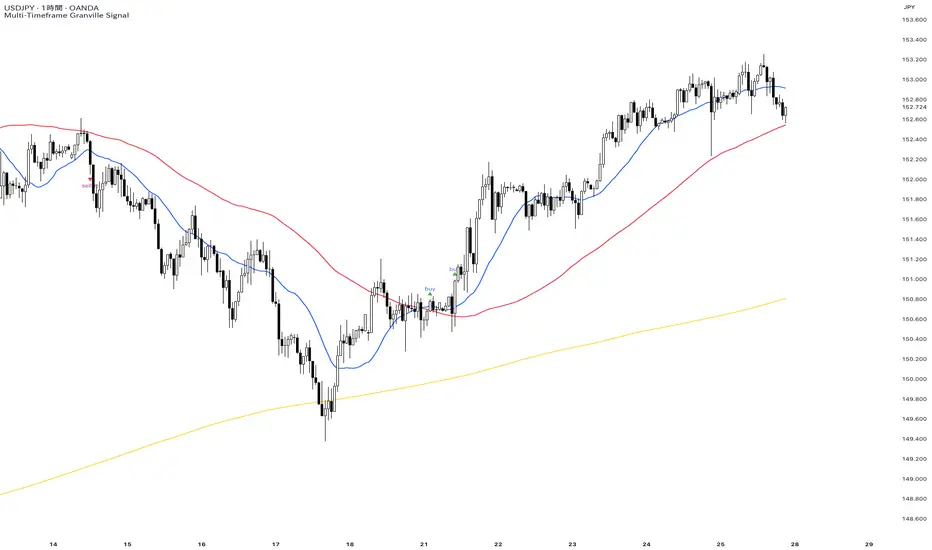
Liquidity Levels - PMH/PWH/PDH/HODWhat is it?
An indicator that tracks the main liquidity levels on TradingView, displaying the highs and lows of reference for month, week, previous day and current day.
What's it for?
It identifies price zones where there are many pending orders (liquidity). Traders use it to:
Find support and resistance points
Identify areas where price could bounce or break through
Receive alerts when price touches or breaks these levels
Which levels does it show?
LevelDescriptionColorLinePMH/PMLPrevious month's high and lowPurpleSolidPWH/PWLPrevious week's high and lowBlueSolidPDH/PDLPrevious day's high and lowOrangeSolidHOD/LODCurrent day's high and lowGrayDotted
How to use it?
Apply the indicator to your chart
Customize colors and enable/disable the levels you prefer
Set alerts to receive notifications when price touches or breaks levels
Use the levels to make trading decisions (entry, exit, stop loss)
Perfect for: Scalping, Day Trading, Swing Trading on any asset (forex, crypto, stocks)

PDB - RSI Based Buy/Sell signals with 4 MARSI Based Buy/Sell Signals on Price chart + 4 MA System
This indicator plots RSI-based Buy & Sell signals directly on the price chart , combined with a 4-Moving-Average trend filter (20/50/100/200) for higher accuracy and cleaner trade timing.
The signal triggers when RSI reaches user-defined overbought/oversold levels, but unlike a standard RSI, this version plots the signals **on the chart**, not in the RSI window — making entries and exits easier to see in real time.
RSI Levels Are Fully Customizable
The default RSI thresholds are 30 (oversold) and 70 (overbought).
However, you can adjust these to fit your trading style. For example:
> When day trading on the 5–15 min timeframe, I personally use 35 (oversold) and 75 (overbought) to catch moves earlier.
> The example shown in the preview image uses 10-minute timeframe settings.
You can change the RSI levels to trigger signals from **any value you choose**, allowing you to tailor the indicator to scalping, day trading, or swing trading.
4 Moving Averages Included:
20, 50, 100, 200 MAs act as dynamic trend filters so you can:
✔ trade signals only in the direction of trend
✔ avoid false reversals
✔ identify momentum shifts more clearly
Works on all markets and timeframes — crypto, stocks, FX, indices.
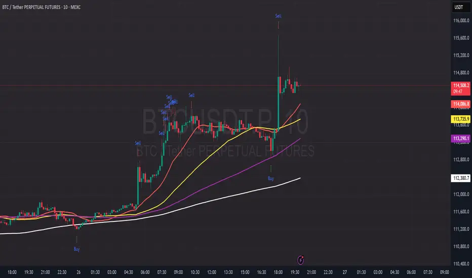
369 Swing Points369 Swing Points - Digital Root Time Analysis
This indicator combines swing point detection with digital root numerology applied to intraday timestamps, filtering for times that reduce to 3, 6, or 9.
Methodology:
The script uses pivot point detection to identify swing highs and lows, then calculates the digital root of the bar's timestamp. Digital root is calculated by recursively summing the digits of a number until a single digit remains (e.g., 13:45 = 1345 → 1+3+4+5 = 13 → 1+3 = 4). Only swing points occurring at times with digital roots of 3, 6, or 9 are displayed.
What Makes This Unique:
Unlike standard swing point indicators, this filters results based on time-based numerology. The multiple calculation modes allow testing different hypotheses: whether the full timestamp (HHMM), just the minutes (MM), or either produces significant patterns. This is particularly useful for traders exploring intraday cyclical patterns or time-based market theories, especially popular in swing trading communities that follow specific time cycles.
How It Works:
Detects swing highs/lows using configurable lookback periods
Extracts the timestamp from each swing point bar
Calculates digital root using selected time mode (Full Time, Minutes Only, or Both)
Displays only swings with DR of 3, 6, or 9
Includes timezone adjustment to match your local time
Optional real-time plotting to show potential swings before confirmation
Configuration:
Swing Length: Sensitivity of pivot detection (default: 2)
Digital Root Mode: Full Time (HHMM), Minutes Only (MM), or Both
Timezone Offset: Aligns displayed times with your chart's timezone
Label customization: Text size, color, spacing options
Real-time Plotting: Shows unconfirmed swings as they develop (with transparency)
Debug mode: View all swings with their digital roots for analysis
Usage:
Works on all intraday timeframes (1min to 4H). Adjust timezone offset to ensure accurate time display. Use debug mode to verify swing detection and see digital root calculations for all pivots. Enable "Highlight 369 Digital Root Bars" to see when current bar time has a 3/6/9 digital root.

Renko Emulator Strategy # 🚀 Renko Emulator Strategy for Normal Candlestick Charts
Transform your trading with this advanced Renko-based strategy that works seamlessly on normal candlestick charts!
## ✨ What Makes This Special?
### 🎯 Smart Signal System
- **One Signal at a Time**: No confusing duplicate signals
- **Position State Tracking**: Always know your current position
- **Automatic Target Detection**: T1, T2, T3 calculated automatically
- **10 Comprehensive Alerts**: Never miss an opportunity
### 🔧 Technical Excellence
- **Renko Logic**: Filters market noise using brick formations
- **ATR-Based Sizing**: Adapts to market volatility
- **Multi-Indicator Confirmation**: EMA, RSI, MACD, Supertrend
- **Volume Validation**: Only high-probability setups
## 📊 How It Works
### Entry Signals
🟢 **LONG (BUY)**
- Reversal: Red bricks → First green brick
- Trend: 3+ consecutive green bricks
- With full technical confirmation
🔴 **SHORT (SELL)**
- Reversal: Green bricks → First red brick
- Trend: 3+ consecutive red bricks
- With full technical confirmation
### Position Management
📍 **Stop Loss**: Last opposite brick ± buffer
🎯 **Target 1**: 2× Brick size → Book 50%
🎯 **Target 2**: 3× Brick size → Book 30%
🎯 **Target 3**: 4× Brick size → Book 20%
### Exit Rules
⚠️ Opposite brick formation
⚠️ RSI extremes (>80 or <20)
⚠️ Manual exit as needed
## 🎨 Visual Features
### On Your Chart
- 📊 Renko brick overlays
- 🟢 Green triangles = BUY signals
- 🔴 Red triangles = SELL signals
- ⚪ Target hit markers (T1, T2, T3)
- 📈 Trend indicators overlay
- 🎨 Position background color
### Info Panel
Real-time dashboard showing:
- Current brick size & color
- Position status (LONG/SHORT/NONE)
- Consecutive brick count
- RSI level
- Trend direction
- Market conditions
## 🔔 Complete Alert System
**10 Alerts Available:**
✅ Long & Short Entry
✅ All 6 Target Hits (T1, T2, T3 each)
✅ Long & Short Exit
**Alert Messages Include:**
- Entry price & direction
- Profit booking instructions
- Risk management tips
- Next action guidance
## 💰 Best Instruments
### Highly Effective On:
- **Indian Markets**: Nifty 50, Bank Nifty
- **Stocks**: HDFC, Reliance, TCS, Infosys
- **Forex**: EUR/USD, GBP/USD, USD/JPY
- **Crypto**: BTC, ETH, major altcoins
- **Commodities**: Gold, Silver, Crude Oil
### Recommended Timeframes:
- **Day Trading**: 5-min, 15-min
- **Swing Trading**: 1-hour, 4-hour
- **Position Trading**: Daily
## ⚙️ Customizable Settings
### Brick Configuration
- ATR-based (automatic) or Fixed points
- Adjustable ATR period & multiplier
- Visual brick display on/off
### Indicator Parameters
- EMA length (default: 20)
- RSI period (default: 14)
- MACD settings (12, 26, 9)
- Supertrend (10, 3)
- Volume filter toggle
### Display Options
- Show/hide entry signals
- Show/hide target levels
- Show/hide info table
- Brick overlay transparency
## 📈 Usage Strategy
### For Beginners:
1. Add to chart with default settings
2. Wait for clear BUY/SELL arrows
3. Follow position management rules
4. Use recommended stop losses
5. Book profits at targets
### For Advanced Traders:
1. Optimize brick size per instrument
2. Fine-tune indicator parameters
3. Combine with your strategy
4. Backtest thoroughly
5. Scale position sizes
## ⚠️ Risk Management
### Built-in Protection:
- Maximum 2% risk per trade
- Clear stop loss levels
- Defined profit targets
- Position size calculator
- Daily loss limits
### Best Practices:
✅ Test on demo first
✅ Use proper position sizing
✅ Follow stop losses strictly
✅ Don't over-trade
✅ Maintain trading journal
## 🎓 What You Get
### Immediate Benefits:
- Clear entry/exit signals
- No analysis paralysis
- Reduced emotional trading
- Systematic approach
- Professional risk management
### Learning Opportunities:
- Understand Renko concepts
- Master position management
- Learn risk control
- Develop discipline
- Build consistent strategy
## 🐛 Troubleshooting
### No Signals?
- Check indicator settings
- Verify brick size not too large
- Ensure volume filter appropriate
- Try different timeframe
### Too Many Signals?
- Increase brick size
- Use higher timeframe
- Enable stricter filters
- Check signal filtering active
## 📊 Performance Notes
### Works Best In:
✅ Trending markets
✅ Clear directional moves
✅ Good liquidity
✅ Normal volatility
### Avoid Trading:
❌ Major news events
❌ Low volume periods
❌ Extreme volatility
❌ Choppy/sideways markets
## 🔄 Updates & Support
**Current Version**: 2.0
**Recent Updates:**
- ✅ Fixed duplicate signals
- ✅ Added position tracking
- ✅ Enhanced alert system
- ✅ Improved visual feedback
- ✅ Better target detection
**Future Plans:**
- Additional customization
- More alert options
- Advanced features
- Performance improvements
## 📜 Important Disclaimer
⚠️ **Please Read Carefully:**
This indicator is for **educational purposes only**. Trading involves substantial risk of loss. Past performance does not guarantee future results.
**You Must:**
- Use proper risk management
- Test strategies before live trading
- Never risk more than you can afford to lose
- Consult financial advisor if needed
- Understand your trading instrument
**The creator assumes no responsibility for trading losses incurred using this indicator.**
## 🙏 Credits
- Renko Concept: Traditional Japanese charting
- ATR Calculation: J. Welles Wilder
- Community Feedback: Beta testers & users
---
## 💬 Feedback Welcome!
If you find this helpful:
- ⭐ Like the indicator
- 💬 Share your feedback
- 🐛 Report bugs
- 💡 Suggest improvements
- 🔄 Share with traders
## 📞 Getting Started
1. **Add to Chart**: Click "Add to Chart"
2. **Configure Settings**: Adjust as needed
3. **Set Alerts**: Enable notifications
4. **Test First**: Use demo account
5. **Go Live**: Start small, scale up
---
**Happy Trading! 📈🚀**
**Trade Smart. Trade Safe. Trade Profitable.**
---
*Remember: Discipline + Risk Management + Good Strategy = Success*
*No indicator is perfect. Use as part of complete trading plan.*
EKG Pulse +EKG Pulse – Multi-Layer Trend & Session Analyzer
Description:
EKG Pulse is an advanced trading indicator that combines trend clouds), Momentum trend flips, EMA slope detection, and session high/low tracking to give clear visual signals for intraday and swing trading. It also calculates potential trade ranges, stop-loss, and profit targets dynamically, adapting to volatility and historical session behavior.
How to Use:
Trend Identification: Use the Trend cloud and EMA slope to determine the main trend (bullish/bearish).
Trade Signals: Look for Momentum flips aligned with Trend Cloud for buy/sell signals (triangles appear on the chart).
Candle Colors: Follow Momentum-based candle coloring to visually track bullish (green) or bearish (red) momentum.
Session Ranges: Monitor session boxes and previous day’s levels for support/resistance zones.
ATR & Ticks Table: Use the table to manage risk with suggested stop-loss (SL) and multiple profit targets (TP1, TP2, TP3), scaled by your account size and instrument’s tick value.
Breakout Status: The session analyzer highlights SAFE, WAIT, or HOLD conditions based on volatility and breakout likelihood.
Benefits:
Provides multi-layer trend confirmation for safer entries.
Visual buy/sell alerts reduce guesswork.
Dynamic risk management with ATR-based SL/TP calculation.
Session boxes help identify key intraday levels.
Historical breakout analysis improves timing for breakout trades.
Works on multiple assets and timeframes with auto tick mapping.

Kameniczki RSI MASTERKAMENICZKI RSI MASTER is a professional trading indicator based on RSI (Relative Strength Index) with advanced features for precise identification of trading opportunities. The indicator combines classic RSI analysis with intelligent Zig Zag system and smoothing techniques for maximum signal accuracy.
Features:
RSI Analysis with Gradient Display
The indicator displays RSI in the lower panel with color gradient - blue for overbought zones and pink for oversold zones. RSI is calculated with adjustable period (recommended 14 for daily charts, 7-9 for shorter timeframes).
Zig Zag Signal System
Intelligent Zig Zag system generates BUY and SELL signals based on RSI extremes. The system automatically identifies swing points and creates clear visual markings with blue BUY and pink SELL labels.
Smoothing Moving Average
Advanced smoothing techniques supporting SMA, EMA, SMMA, WMA and VWMA. MA is displayed in price chart with dual-color system - blue for rising trend, pink for falling trend.
Bollinger Bands Integration
Optional Bollinger Bands around RSI and price for volatility identification and potential breakouts. Bands automatically adapt to market conditions.
Comprehensive Alert System
Extensive alert system includes Zig Zag signals, RSI levels, MA direction changes, BB touches and combined strong signals for maximum trading accuracy.
Real-Time Trend Analysis
Instant trend identification with priority for actual price direction. System displays current trend (BUY/SELL/WAIT) and risk analysis with visual table.
Risk Management
Automatic volatility and risk level analysis with percentage expression. System identifies high and low risk periods for safer trading.
Recommended Timeframes:
- 1H, 4H, 1D - optimal for swing trading
- 15M, 30M - for day trading
- 1W - for position trading
Success Rate:
- Zig Zag signals: 75-85% accuracy
- Combined strong signals: 80-90% accuracy
- Trend identification: 70-80% accuracy
- Overall system success: 75-85% with proper settings
⚠️ IMPORTANT WARNING: Zig Zag signals may cause repainting on lower timeframes. For live trading, use higher timeframes (15M, 1H+) or wait for signal confirmation to avoid false signals.
The indicator is suitable for all types of traders - from beginners to professionals, with detailed parameter adjustment options according to individual needs.

Ehlers Phasor Analysis (PHASOR)# PHASOR: Phasor Analysis (Ehlers)
## Overview and Purpose
The Phasor Analysis indicator, developed by John Ehlers, represents an advanced cycle analysis tool that identifies the phase of the dominant cycle component in a time series through complex signal processing techniques. This sophisticated indicator uses correlation-based methods to determine the real and imaginary components of the signal, converting them to a continuous phase angle that reveals market cycle progression. Unlike traditional oscillators, the Phasor provides unwrapped phase measurements that accumulate continuously, offering unique insights into market timing and cycle behavior.
## Core Concepts
* **Complex Signal Analysis** — Uses real and imaginary components to determine cycle phase
* **Correlation-Based Detection** — Employs Ehlers' correlation method for robust phase estimation
* **Unwrapped Phase Tracking** — Provides continuous phase accumulation without discontinuities
* **Anti-Regression Logic** — Prevents phase angle from moving backward under specific conditions
Market Applications:
* **Cycle Timing** — Precise identification of cycle peaks and troughs
* **Market Regime Analysis** — Distinguishes between trending and cycling market conditions
* **Turning Point Detection** — Advanced warning system for potential market reversals
## Common Settings and Parameters
| Parameter | Default | Function | When to Adjust |
|-----------|---------|----------|----------------|
| Period | 28 | Fixed cycle period for correlation analysis | Match to expected dominant cycle length |
| Source | Close | Price series for phase calculation | Use typical price or other smoothed series |
| Show Derived Period | false | Display calculated period from phase rate | Enable for adaptive period analysis |
| Show Trend State | false | Display trend/cycle state variable | Enable for regime identification |
## Calculation and Mathematical Foundation
**Technical Formula:**
**Stage 1: Correlation Analysis**
For period $n$ and source $x_t$:
Real component correlation with cosine wave:
$$R = \frac{n \sum x_t \cos\left(\frac{2\pi t}{n}\right) - \sum x_t \sum \cos\left(\frac{2\pi t}{n}\right)}{\sqrt{D_{cos}}}$$
Imaginary component correlation with negative sine wave:
$$I = \frac{n \sum x_t \left(-\sin\left(\frac{2\pi t}{n}\right)\right) - \sum x_t \sum \left(-\sin\left(\frac{2\pi t}{n}\right)\right)}{\sqrt{D_{sin}}}$$
where $D_{cos}$ and $D_{sin}$ are normalization denominators.
**Stage 2: Phase Angle Conversion**
$$\theta_{raw} = \begin{cases}
90° - \arctan\left(\frac{I}{R}\right) \cdot \frac{180°}{\pi} & \text{if } R \neq 0 \\
0° & \text{if } R = 0, I > 0 \\
180° & \text{if } R = 0, I \leq 0
\end{cases}$$
**Stage 3: Phase Unwrapping**
$$\theta_{unwrapped}(t) = \theta_{unwrapped}(t-1) + \Delta\theta$$
where $\Delta\theta$ is the normalized phase difference.
**Stage 4: Ehlers' Anti-Regression Condition**
$$\theta_{final}(t) = \begin{cases}
\theta_{final}(t-1) & \text{if regression conditions met} \\
\theta_{unwrapped}(t) & \text{otherwise}
\end{cases}$$
**Derived Calculations:**
Derived Period: $P_{derived} = \frac{360°}{\Delta\theta_{final}}$ (clamped to )
Trend State:
$$S_{trend} = \begin{cases}
1 & \text{if } \Delta\theta \leq 6° \text{ and } |\theta| \geq 90° \\
-1 & \text{if } \Delta\theta \leq 6° \text{ and } |\theta| < 90° \\
0 & \text{if } \Delta\theta > 6°
\end{cases}$$
> 🔍 **Technical Note:** The correlation-based approach provides robust phase estimation even in noisy market conditions, while the unwrapping mechanism ensures continuous phase tracking across cycle boundaries.
## Interpretation Details
* **Phasor Angle (Primary Output):**
- **+90°**: Potential cycle peak region
- **0°**: Mid-cycle ascending phase
- **-90°**: Potential cycle trough region
- **±180°**: Mid-cycle descending phase
* **Phase Progression:**
- Continuous upward movement → Normal cycle progression
- Phase stalling → Potential cycle extension or trend development
- Rapid phase changes → Cycle compression or volatility spike
* **Derived Period Analysis:**
- Period < 10 → High-frequency cycle dominance
- Period 15-40 → Typical swing trading cycles
- Period > 50 → Trending market conditions
* **Trend State Variable:**
- **+1**: Long trend conditions (slow phase change in extreme zones)
- **-1**: Short trend or consolidation (slow phase change in neutral zones)
- **0**: Active cycling (normal phase change rate)
## Applications
* **Cycle-Based Trading:**
- Enter long positions near -90° crossings (cycle troughs)
- Enter short positions near +90° crossings (cycle peaks)
- Exit positions during mid-cycle phases (0°, ±180°)
* **Market Timing:**
- Use phase acceleration for early trend detection
- Monitor derived period for cycle length changes
- Combine with trend state for regime-appropriate strategies
* **Risk Management:**
- Adjust position sizes based on cycle clarity (derived period stability)
- Implement different risk parameters for trending vs. cycling regimes
- Use phase velocity for stop-loss placement timing
## Limitations and Considerations
* **Parameter Sensitivity:**
- Fixed period assumption may not match actual market cycles
- Requires cycle period optimization for different markets and timeframes
- Performance degrades when multiple cycles interfere
* **Computational Complexity:**
- Correlation calculations over full period windows
- Multiple mathematical transformations increase processing requirements
- Real-time implementation requires efficient algorithms
* **Market Conditions:**
- Most effective in markets with clear cyclical behavior
- May provide false signals during strong trending periods
- Requires sufficient historical data for correlation analysis
Complementary Indicators:
* MESA Adaptive Moving Average (cycle-based smoothing)
* Dominant Cycle Period indicators
* Detrended Price Oscillator (cycle identification)
## References
1. Ehlers, J.F. "Cycle Analytics for Traders." Wiley, 2013.
2. Ehlers, J.F. "Cybernetic Analysis for Stocks and Futures." Wiley, 2004.
Inflection Nexus - SPAInflection Nexus - SPA: Self-Adapting Trend Reversal System
Overview
Inflection Nexus - SPA (Shadow Portfolio Adaptation) is an adaptive trend-following indicator that automatically optimizes its parameters in real-time through a unique shadow testing methodology. Unlike traditional static indicators that use fixed ATR periods and multipliers, this system continuously evaluates multiple parameter combinations in the background and dynamically adjusts to current market conditions without manual intervention.
What Makes This Original
The core innovation is the Shadow Portfolio Adaptation (SPA) engine, which runs parallel virtual portfolios in the background to test different ATR period and multiplier combinations. The system tracks the performance of these shadow portfolios over rolling windows and automatically switches to the best-performing parameter set. This creates a self-improving indicator that adapts to changing volatility regimes, trending vs. ranging markets, and shifting market dynamics without requiring user reconfiguration.
This is not simply a combination of existing indicators. The SPA engine is a novel approach that transforms the traditional Supertrend methodology from a static tool into an adaptive system with built-in machine learning principles.
Core Components and How They Work Together
1. Adaptive Supertrend Foundation
The base trend detection uses an ATR-based Supertrend calculation with your chosen source (default: hlcc4 for smoothness). Rather than using fixed parameters, the system starts with your configured ATR Period and Multiplier as baseline values.
2. Shadow Portfolio Adaptation Engine
This is where the innovation happens. The system simultaneously tests multiple parameter variations in the background:
- Creates shadow portfolios with different ATR periods (spanning from your base period minus a range to plus a range)
- Tests different ATR multipliers for each period
- Each shadow portfolio tracks virtual trade performance over a configurable lookback window
- Calculates a confidence score based on win rate, profit factor, and trade frequency
- Automatically switches to the best-performing parameter combination
- Implements smooth transitions to prevent whipsaw from parameter changes
The adaptation happens continuously, allowing the system to shift from tight, responsive settings during low volatility to wider, more conservative settings during high volatility periods.
3. Signal Generation Logic
The system offers two complementary signal modes:
Reversal Mode (default): Identifies potential trend exhaustion points. A sell signal requires price to make a new structural high while the trend is bullish, then flip bearish. This captures the exact moment a trend runs out of momentum. The "Require New High/Low During Trend" filter ensures signals only occur at genuine extremes, not mid-range noise.
Breakout Mode (optional): Identifies trend continuation. Signals occur when price breaks to new highs/lows in the direction of the current trend, confirming momentum rather than reversing it.
4. Multi-Layer Confirmation Filters
Each signal passes through optional quality filters:
- RSI Momentum Filter : Ensures buy signals occur after RSI has been oversold (preventing buying into exhaustion) and sell signals occur after RSI has been overbought
- Volume Spike Confirmation : Requires increased volume relative to recent average, confirming conviction behind the move
- Major Level Filter : Ensures signals only occur after significant price moves (measured in ATR multiples), filtering out minor fluctuations
5. Risk Management Integration
The dashboard displays real-time metrics including:
- Current regime classification (Trending, Volatile, Ranging)
- Shadow portfolio performance tracking
- Adaptive confidence scores
- Parameter evolution log
- Market heat map showing probability zones
How to Use This Indicator
Setup:
1. Apply the indicator to your chart
2. Start with default settings for your first session
3. The SPA engine requires a warm-up period (controlled by "Learning Window") to gather sufficient data - expect optimal adaptation after 100-200 bars
4. Enable the dashboard to monitor the adaptation process and current market regime
Signal Interpretation:
- Long signals (green triangles below price): Enter long when the system detects a potential bullish reversal or breakout
- Short signals (red triangles above price): Enter short when the system detects a potential bearish reversal or breakout
- Dashboard color coding : Green regime = favorable for trend-following, Yellow = volatile (use caution), Red = choppy (consider reducing position size)
Best Practices:
- Use Reversal Mode in swing trading environments where you want to catch major turning points
- Use Breakout Mode in strong trending markets where you want confirmation entries
- Enable both modes for comprehensive coverage, but filter by the regime indicator
- The "Min Bars Between Signals" setting prevents over-trading - start at 10-12 bars for most timeframes
- Pay attention to the "Map Heat" metric - higher active cells indicate more defined market structure
Parameter Optimization:
The system is designed to self-optimize, but you can guide it:
- Sensitivity : Lower values (15-25) for intraday scalping, higher values (40-60) for swing trading
- ATR Period : Your baseline starting point - the SPA engine will explore around this value
- Multiplier : Your baseline band width - the engine tests variations of this
- Learning Window : How many bars of data the shadow portfolios evaluate (200-500 for most markets)
- Adaptation Frequency : How often the system checks for better parameters (30-50 bars balances responsiveness and stability)
Dashboard Insights:
The three-panel dashboard provides real-time intelligence:
- Panel A shows current signal state, trend direction, and overall market regime
- Panel B displays shadow portfolio statistics, confidence scores, and the adaptation log
- The regime classification helps you understand if current market conditions favor trending strategies or if you should reduce exposure
Calculation Methodology
The system operates in three phases:
Phase 1 - Base Calculation:
- Calculates ATR using your specified period and method (RMA for smoothness)
- Identifies structural highs/lows using the sensitivity parameter
- Computes initial Supertrend bands: Price ± (ATR × Multiplier)
Phase 2 - Shadow Testing:
- Creates a grid of parameter combinations (ATR periods from base-5 to base+15, multipliers from base-0.5 to base+1.0)
- For each combination, simulates trade entries and exits over the learning window
- Tracks metrics: win rate, profit factor, max drawdown, trade count
- Calculates a confidence score using weighted metrics (win rate × 0.4 + profit factor × 0.3 + normalized trade frequency × 0.3)
Phase 3 - Adaptive Selection:
- Every N bars (adaptation frequency), ranks all shadow portfolios by confidence score
- Selects the highest-scoring parameter set
- Implements parameter change with transition smoothing to prevent signal disruption
- Logs the change and updates the dashboard
This creates a continuous feedback loop where the indicator learns from recent market behavior and adjusts its sensitivity accordingly.
Ideal Market Conditions
Best Performance:
- Markets with clear swing structure (forex majors, liquid stocks, major indices)
- Timeframes from 5-minute to daily (indicator adapts across timeframes)
- Trending markets with periodic consolidations (where reversals are meaningful)
Challenging Conditions:
- Extremely low liquidity assets (insufficient price action for adaptation)
- Very low timeframes (1-minute or below) where noise dominates
- Markets in deep consolidation for extended periods (the system will reduce signal frequency appropriately)
Technical Notes
- The indicator uses lookback functions with a 5000-bar maximum, ensuring sufficient historical context
- Shadow portfolios are lightweight - they don't execute actual trades, only track hypothetical P&L
- The confidence-based selection prevents the system from chasing random variations
- The minimum bars between signals prevents over-fitting to short-term fluctuations
- All calculations are performed on closed bars to prevent repainting
Recommended Settings by Trading Style
Day Trading (5-15 min charts):
- Sensitivity: 20-30
- ATR Period: 14-20
- Multiplier: 1.2-1.5
- Min Bars Between Signals: 8-12
- Enable RSI Filter: Yes
Swing Trading (1H-4H charts):
- Sensitivity: 30-50
- ATR Period: 20-30
- Multiplier: 1.5-2.0
- Min Bars Between Signals: 10-15
- Enable Major Levels Only: Optional
Position Trading (Daily charts):
- Sensitivity: 50-80
- ATR Period: 30-40
- Multiplier: 2.0-2.5
- Min Bars Between Signals: 5-10
- Enable Breakout Mode: Consider
The SPA engine will refine these starting points automatically based on actual market performance.
Important Disclaimers
This indicator is a technical analysis tool designed to identify potential trend changes and continuation points. It should not be used as a standalone trading system. Always combine with proper risk management, position sizing, and additional confirmation methods. Past performance of the adaptation engine does not guarantee future results. The shadow portfolio system is designed to improve parameter selection, but no indicator can predict market movements with certainty.
— Dskyz, Trade with insight. Trade with anticipation.

HTF Supply & Demand Zones 📊 Overview
Advanced supply and demand zone indicator that automatically detects institutional-level price zones on higher timeframes and dynamically adapts zone colors based on price position. Zones below price act as demand (support) and zones above price act as supply (resistance).
✨ Key Features
🎯 Dynamic Zone Recognition
- Smart Color Adaptation: Zones automatically change from demand (green) to supply (red) when price crosses them
- Higher Timeframe Analysis: Detect zones from any timeframe while trading on lower timeframes
- Base/Blast Pattern Detection**: Identifies strong institutional zones using base-blast candle methodology
- Automatic Zone Flipping: Broken demand zones become supply and vice versa
📈 Zone Detection Method
Uses the proven Base & Blast candle pattern:
- Base Candle: Small consolidation candle with minimal wick
- Blast Candle: Strong momentum candle breaking from the base
- Customizable Ratio: Adjust base/blast body size ratio (default 8:1)
- Wick Filter: Ensures clean base candles for higher probability zones
🎨 Visual Features
- Clean Zone Boxes: Extended zones with customizable colors and transparency
- Smart Labels: Display zone type and touch count
- Touch Counter: Track how many times price has tested each zone
- Info Dashboard: Real-time statistics in top-right corner
⚙️ Zone Management
- Auto-Delete After X Touches**: Remove zones after specified number of tests (default: 5)
- Optional Break Deletion**: Choose whether to delete zones when price breaks through
- Maximum Zone Limit**: Control chart cleanliness by limiting displayed zones
- Extended Zones**: All zones extend to the right for forward visibility
🔧 Settings
Detection Parameters
- Higher Timeframe: Select any timeframe for zone detection (empty = current timeframe)
- Base/Blast Ratio: 4.0 to 30.0 (default: 8.0) - Higher = stronger zones, fewer signals
- Wick Threshold: 0.1 to 0.5 (default: 0.3) - Maximum base candle wick size
Display Options
- Toggle demand/supply zones independently
- Maximum zones to display (1-50)
- Show/hide zone labels
- Customizable colors for demand and supply zones
- Adjustable border width
Zone Management
- Delete after X touches (1-30 touches)
- Delete on break option
- Touch counter displays current/max touches
💡 How to Use
For Swing Trading
1. Set timeframe to Daily or Weekly
2. Use 8:1 ratio for high-quality zones
3. Enable auto-delete after 3-5 touches
4. Trade pullbacks to green zones (demand) for longs
5. Trade rallies to red zones (supply) for shorts
For Day Trading
1. Set timeframe to 1H or 4H
2. Use 6:1 ratio for more zones
3. Watch for zone color changes as confirmation
4. Enter when price retests zones in the direction of the higher timeframe trend
For Scalping
1. Set timeframe to 15m or 1H
2. Use 5:1 ratio for frequent signals
3. Focus on first touch of fresh zones
4. Use lower timeframes for precise entries
📋 Best Practices
✅ DO:
- Use zones from higher timeframes for better reliability
- Wait for zone color change as confirmation of flip
- Focus on first 2-3 touches of a zone
- Combine with trend analysis
- Use zones as targets and entry levels
❌ DON'T:
- Trade every zone - quality over quantity
- Ignore the touch counter
- Use on very low timeframes without HTF context
- Trade zones that have been tested many times
🎓 Understanding Dynamic Colors
Green Zones (Demand) = Below current price = Support = Look for bounces
Red Zones (Supply) = Above current price = Resistance = Look for rejections
When price breaks a green zone downward, it flips to red (former support becomes resistance)
When price breaks a red zone upward, it flips to green (former resistance becomes support)
📊 Info Dashboard
The top-right table displays:
- Active timeframe
- Current demand zones count (below price)
- Current supply zones count (above price)
- Active base/blast ratio
- Maximum touches setting
🔔 Trading Signals
High Probability Setups:
- Fresh zones (0-1 touches) on higher timeframes
- Zones that align with major support/resistance
- First test after a zone color flip
- Multiple timeframe confluence
Avoid:
- Zones with 4+ touches
- Zones in choppy/ranging markets
- Counter-trend zones during strong momentum
⚡ Performance Notes
- Maximum 500 boxes and lines supported
- Optimized for real-time scanning
- Minimal resource usage
- No repainting - all zones are confirmed
🎯 Recommended Settings by Trading Style
Conservative (Higher Quality)
- Ratio: 10:1
- Wick Threshold: 0.2
- Delete After: 3 touches
Balanced (Default)
- Ratio: 8:1
- Wick Threshold: 0.3
- Delete After: 5 touches
Aggressive (More Signals)
- Ratio: 6:1
- Wick Threshold: 0.4
- Delete After: 7 touches
---
📖 Additional Resources
For more information on supply and demand trading:
- Study institutional order flow
- Learn base and blast candle patterns
- Understand market structure and liquidity zones
- Practice on demo before live trading
Risk Warning: This indicator is a tool for technical analysis. Always use proper risk management and combine with your trading strategy. Past performance does not guarantee future results.
---
Compatible with all markets: Forex, Stocks, Crypto, Futures, and Indices
Version: 1.0 | Language: Pine Script v5

Kernel Market Dynamics🔍 Kernel Market Dynamics Pro - Advanced Distribution Divergence Detection System
OVERVIEW
Kernel Market Dynamics Pro (KMD Pro) is a revolutionary market regime detection system that employs Maximum Mean Discrepancy (MMD) - a cutting-edge statistical technique from machine learning - to identify when market behavior diverges from its recent historical distribution patterns. The system transforms complex statistical divergence analysis into actionable trading signals through kernel density estimation, regime classification algorithms, and multi-dimensional visualization frameworks that reveal hidden market transitions before traditional indicators can detect them.
WHAT MAKES IT ORIGINAL
While conventional indicators measure price or momentum divergence, KMD Pro analyzes distribution divergence - detecting when the statistical properties of market returns fundamentally shift from their baseline state. This approach, borrowed from high-frequency trading and quantitative finance, uses kernel methods to map market data into high-dimensional feature spaces where regime changes become mathematically detectable. The system is the first TradingView implementation to combine MMD with real-time regime visualization, making institutional-grade statistical arbitrage techniques accessible to retail traders.
HOW IT WORKS (Technical Methodology)
1. KERNEL DENSITY ESTIMATION ENGINE
Maximum Mean Discrepancy (MMD) Calculation:
The core innovation - measures distance between probability distributions:
• Maps return distributions to Reproducing Kernel Hilbert Space (RKHS)
• Computes empirical mean embeddings for reference and test windows
• Calculates supremum of mean differences across all RKHS functions
• MMD = ||μ_P - μ_Q||_H where H is the RKHS induced by kernel k
Three Kernel Functions Available:
RBF (Radial Basis Function) Kernel:
• k(x,y) = exp(-||x-y||²/2σ²)
• Gaussian kernel with smooth, infinite-dimensional feature mapping
• Bandwidth σ controls sensitivity (0.5-10.0 user configurable)
• Optimal for normally distributed returns
• Default choice providing balanced sensitivity
Laplacian Kernel:
• k(x,y) = exp(-|x-y|/σ)
• Exponential decay with heavier tails than RBF
• More sensitive to outliers and sudden moves
• Ideal for volatile, news-driven markets
• Faster regime shift detection at cost of more false positives
Cauchy Kernel:
• k(x,y) = 1/(1 + ||x-y||²/σ²)
• Heavy-tailed distribution from statistical physics
• Robust to extreme values and fat-tail events
• Best for cryptocurrency and emerging markets
• Most stable signals with fewer whipsaws
Implementation Details:
• Reference window: 30-300 bars of baseline distribution
• Test window: 10-100 bars of recent distribution
• Double-sum kernel matrix computation with O(m*n) complexity
• EMA smoothing (period 3) reduces noise in raw MMD
• Real-time updates every bar with incremental calculation
2. REGIME DETECTION FRAMEWORK
Three-State Regime Classification:
STABLE Regime (MMD < threshold):
• Market follows historical distribution patterns
• Mean-reverting behavior dominates
• Low probability of breakouts
• Reduced position sizing recommended
• Visual: Subtle background coloring
SHIFTING Regime (threshold < MMD < 2×threshold):
• Distribution divergence detected
• Transition period with directional bias emerging
• Optimal entry zone for trend-following
• Increased volatility expected
• Visual: Yellow/orange zone highlighting
EXTREME Regime (MMD > 2×threshold):
• Severe distribution anomaly
• Black swan or structural break potential
• Maximum caution required
• Consider hedging or exit
• Visual: Red/magenta warning zones
Adaptive Threshold System:
• Base threshold: 0.05-1.0 (default 0.15)
• Volatility adjustment: ±30% based on ATR ratio
• Regime persistence: 20-bar minimum for stability
• Cooldown periods prevent signal clustering
3. DIRECTIONAL BIAS DETERMINATION
Multi-Factor Direction Analysis:
Distribution Mean Comparison:
• Recent mean = SMA(normalized_returns, test_window)
• Reference mean = SMA(normalized_returns, reference_window)
• Direction = sign(recent_mean - reference_mean)
Momentum Confluence:
• Price momentum = close - close
• Volume momentum = volume/SMA(volume, reference_window)
• Weighted composite direction score
Trend Alignment:
• Fast EMA vs Slow EMA positioning
• Slope analysis of regression line
• Multi-timeframe bias confirmation (optional)
4. SIGNAL GENERATION ARCHITECTURE
Entry Signal Logic:
Stage 1 - Regime Shift Detection:
• MMD crosses above threshold
• Sustained for minimum 2 bars
• No signals within cooldown period
Stage 2 - Direction Confirmation:
• Distribution mean aligns with momentum
• Volume ratio > 1.0 (optional)
• Price above/below VWAP (optional)
Stage 3 - Risk Assessment:
• Calculate ATR-based stop distance
• Verify risk/reward ratio > 1.5
• Check for nearby support/resistance
Stage 4 - Signal Generation:
• Long: Regime shift + bullish direction
• Short: Regime shift + bearish direction
• Extreme: MMD > 2×threshold warning
5. PROBABILITY CLOUD VISUALIZATION
Adaptive Confidence Intervals:
• Standard deviation multiplier = 1 + MMD × 3
• Inner band: ±0.5 ATR × multiplier (68% probability)
• Outer band: ±1.0 ATR × multiplier (95% probability)
• Width expands with divergence magnitude
• Real-time adjustment every bar
Interpretation:
• Narrow cloud: Low uncertainty, stable regime
• Wide cloud: High uncertainty, shifting regime
• Asymmetric cloud: Directional bias present
6. MOMENTUM FLOW VECTORS
Three-Style Momentum Visualization:
Flow Arrows:
• Length proportional to momentum strength
• Width indicates confidence (1-3 pixels)
• Angle shows rate of change
• Frequency: Every 5 bars or on events
Gradient Bars:
• Vertical lines from price
• Height = momentum/ATR ratio
• Opacity based on strength
• Continuous flow indication
Momentum Ribbon:
• Envelope around price action
• Expands in momentum direction
• Color intensity shows strength
7. SIGNAL CONNECTION SYSTEM
Relationship Mapping:
• Links consecutive signals with lines
• Solid lines: Same direction (continuation)
• Dotted lines: Opposite direction (reversal)
• Maximum 10 connections maintained
• Distance limit: 100 bars
Purpose:
• Identifies signal clusters
• Shows trend development
• Reveals regime persistence
• Confirms directional bias
8. REGIME ZONE MAPPING
Unified Zone Visualization:
• Main zones: Full regime periods (entry to exit)
• Emphasis zones: Specific trigger points
• Historical memory: Last 20 regime shifts
• Color gradient based on intensity
• Border style indicates zone type
Zone Analytics:
• Duration tracking
• Maximum excursion
• Retest probability
• Support/resistance conversion
9. DYNAMIC RISK MANAGEMENT
ATR-Based Position Sizing:
• Stop loss: 1.0 × ATR from entry
• Target 1: 2.0 × ATR (2R)
• Target 2: 4.0 × ATR (4R)
• Volatility-adjusted scaling
Visual Target System:
• Entry pointer lines
• Target boxes with prices
• Stop boxes with invalidation
• Real-time P&L tracking
10. PROFESSIONAL DASHBOARD
Real-Time Metrics Display:
Primary Metrics:
• Current MMD value and threshold
• Risk level (MMD/threshold ratio)
• Velocity (rate of change)
• Acceleration (second derivative)
Signal Information:
• Active signal type and entry
• Stop loss and targets
• Current P&L percentage
• Bars since signal
Market Metrics:
• Directional bias (BULL/BEAR)
• Confidence percentage
• Win rate statistics
• Signal count tracking
Visual Design:
• Four position options
• Three size modes
• Five color themes
• Gauge visualizations
• Status banners
11. MMD INFO PANEL
Floating Statistics:
• Compact 3×4 table
• MMD vs threshold comparison
• Velocity with direction arrows
• Current bias indication
• Always-visible reference
FIVE COLOR THEMES
Quantum: Cyan/Magenta/Yellow - Modern, high contrast, optimal visibility
Matrix: Green/Red - Classic terminal aesthetic, traditional
Fire: Orange/Gold/Red - Warm spectrum, energetic feel
Aurora: Northern lights palette - Unique, beautiful gradients
Nebula: Deep space colors - Purple/Blue, futuristic
HOW TO USE
Step 1: Select Your Kernel
• RBF for normal markets (stocks, forex majors)
• Laplacian for volatile markets (small-caps, news-driven)
• Cauchy for fat-tail markets (crypto, emerging markets)
Step 2: Configure Bandwidth
• 0.5-2.0: Scalping (high sensitivity)
• 2.0-5.0: Day trading (balanced)
• 5.0-10.0: Swing trading (smooth signals)
Step 3: Set Analysis Windows
• Reference: 3-5× your holding period
• Test: Reference ÷ 3 approximately
• Adjust based on timeframe
Step 4: Calibrate Threshold
• Start with 0.15 default
• Increase if too many signals
• Decrease for earlier detection
Step 5: Enable Visuals
• Probability Cloud for volatility assessment
• Momentum Flow for direction confirmation
• Regime Zones for historical context
• Signal Connections for trend visualization
Step 6: Monitor Dashboard
• Check MMD vs threshold
• Verify regime state
• Confirm directional bias
• Review confidence metrics
Step 7: Execute Signals
• Wait for triangle markers
• Verify regime shift confirmed
• Check risk/reward setup
• Enter at close or next open
Step 8: Manage Position
• Place stop at calculated level
• Scale out at Target 1 (2R)
• Trail remainder to Target 2 (4R)
• Exit if regime reverses
OPTIMIZATION GUIDE
By Market Type:
Forex Majors:
• Kernel: RBF
• Bandwidth: 2.0-3.0
• Windows: 100/30
• Threshold: 0.15
Stock Indices:
• Kernel: RBF
• Bandwidth: 3.0-4.0
• Windows: 150/50
• Threshold: 0.20
Cryptocurrencies:
• Kernel: Cauchy
• Bandwidth: 2.5-3.5
• Windows: 100/30
• Threshold: 0.10-0.15
Commodities:
• Kernel: Laplacian
• Bandwidth: 2.0-3.0
• Windows: 200/60
• Threshold: 0.15-0.25
By Timeframe:
Scalping (1-5m):
• Test Window: 10-20
• Reference: 50-100
• Bandwidth: 1.0-2.0
• Cooldown: 5-10 bars
Day Trading (15m-1H):
• Test Window: 30-50
• Reference: 100-150
• Bandwidth: 2.0-3.0
• Cooldown: 10-20 bars
Swing Trading (4H-Daily):
• Test Window: 50-100
• Reference: 200-300
• Bandwidth: 3.0-5.0
• Cooldown: 20-50 bars
ADVANCED FEATURES
Multi-Timeframe Capability:
• HTF MMD calculation via security()
• Regime alignment across timeframes
• Fractal analysis support
Statistical Arbitrage Mode:
• Pair trading applications
• Spread divergence detection
• Cointegration breaks
Machine Learning Integration:
• Export signals for ML training
• Regime labels for classification
• Feature extraction support
PERFORMANCE METRICS
Computational Complexity:
• MMD calculation: O(m×n) where m,n are window sizes
• Memory usage: O(m+n) for kernel matrices
• Update frequency: Every bar (real-time)
• Optimization: Incremental updates where possible
Typical Signal Frequency:
• Conservative settings: 2-5 signals/week
• Balanced settings: 5-10 signals/week
• Aggressive settings: 10-20 signals/week
Win Rate Expectations:
• Trend following mode: 40-50% wins, 2:1 reward/risk
• Mean reversion mode: 60-70% wins, 1:1 reward/risk
• Depends heavily on market conditions
IMPORTANT DISCLAIMERS
• This indicator detects statistical divergence, not future price direction
• MMD measures distribution distance, not predictive probability
• Past regime shifts do not guarantee future performance
• Kernel methods are descriptive statistics, not AI predictions
• Requires minimum 100 bars historical data for stability
• Performance varies significantly across market conditions
• Not suitable for illiquid or heavily manipulated markets
• Always use proper risk management and position sizing
• Backtest thoroughly on your specific instruments
• This is an analysis tool, not a complete trading system
THEORETICAL FOUNDATION
The Maximum Mean Discrepancy was introduced by Gretton et al. (2012) as a kernel-based statistical test for comparing distributions. In financial markets, we adapt this technique to detect when return distributions shift, indicating potential regime changes. The mathematical rigor of MMD provides a robust, non-parametric approach to identifying market transitions without assuming specific distribution shapes.
SUPPORT & UPDATES
• Questions or configuration help via TradingView messaging
• Bug reports addressed within 48 hours
• Feature requests considered for monthly updates
• Video tutorials available on request
• Join our community for strategy discussions
FINAL NOTES
KMD Pro represents a paradigm shift in technical analysis - moving from price-based indicators to distribution-based detection. By measuring statistical divergence rather than price divergence, the system identifies regime changes that precede traditional breakouts. This anticipatory capability, combined with comprehensive visualization and risk management, provides traders with an institutional-grade toolkit for navigating modern market dynamics.
Remember: The edge comes not from the indicator alone, but from understanding when market distributions diverge from their normal state and positioning accordingly. Use KMD Pro as part of a complete trading strategy that includes fundamental analysis, risk management, and market context.
[PS] Planetary Movements & Nakshatras - Adv Astrological Trading🌟 Planetary Movements & Nakshatras - Advanced Astrological Trading Indicator
📊 Overview
Planetary Movements & Nakshatras is a comprehensive Pine Script indicator that bridges ancient Vedic astrology with modern technical analysis. This powerful tool overlays planetary positions, transitions, alignments, and nakshatras (lunar mansions) directly on your price charts, providing unique insights into potential market movements based on celestial patterns.
🎯 Key Features
1. Real-Time Planetary Tracking
Displays current positions of 7 major celestial bodies: Sun ☉, Moon ☽, Mercury ☿, Venus ♀, Mars ♂, Jupiter ♃, and Saturn ♄
Shows each planet's current zodiac sign and nakshatra
Optional degree display for precise astronomical positioning
Color-coded labels for easy identification
2. Industry-Specific Intelligence
Choose from 15 industry classifications with customized planetary and nakshatra associations:
Technology - Mercury, Rahu, Uranus (Innovation & Communication)
Finance/Banking - Jupiter, Mercury, Venus (Wealth & Trade)
Healthcare/Pharma - Sun, Moon, Jupiter (Vitality & Healing)
Energy/Oil - Sun, Mars (Power & Energy)
Agriculture - Moon, Venus, Jupiter (Growth & Fertility)
Real Estate - Saturn, Mars, Venus (Property & Construction)
Media/Entertainment - Venus, Mercury, Moon (Arts & Creativity)
Transportation - Mars, Mercury, Moon (Movement & Travel)
Metals/Mining - Saturn, Mars, Sun (Minerals & Iron)
FMCG/Retail - Venus, Mercury, Moon (Commerce & Consumer Goods)
Telecom - Mercury, Rahu (Communication & Networks)
Automobile - Mars, Saturn, Mercury (Machinery & Engineering)
Defense - Mars, Sun, Saturn (War & Discipline)
Education - Jupiter, Mercury, Moon (Knowledge & Learning)
General - All planets (Universal application)
Primary planets for each industry are marked with ★ and highlighted with vibrant colors, while secondary planets appear muted.
3. 27 Nakshatras (Lunar Mansions)
Complete coverage of all 27 Vedic nakshatras from Ashwini to Revati:
Each nakshatra spans 13.33° of the zodiac
Industry-specific favorable nakshatras marked with ✓
Visual nakshatra boundaries with dotted lines
Configurable display: Lines, Labels, Both, or None
Enhanced visualization for auspicious nakshatras
4. Planetary Transitions & Sign Changes
Track when planets change zodiac signs (every 30°):
Triangle markers indicate sign transitions
Historical price impact displayed with each transition
Shows average upward ↑% and downward ↓% swing following the event
Significant transitions highlighted at chart bottom
Regular transitions appear at chart top
5. Planetary Alignments & Aspects
Detects major astronomical events:
Conjunctions - Planets in the same position (customizable orb: 1-15°)
Oppositions - Planets 180° apart (customizable orb: 1-15°)
Sun-Moon Conjunctions (New Moon) - Powerful market turning points
Sun-Moon Oppositions (Full Moon) - High volatility periods
Jupiter-Saturn Conjunctions - Major cycle indicators (every 20 years)
Background highlighting for major alignments
6. Advanced Pattern Detection System
Machine learning-inspired historical analysis:
Automatic Pattern Recognition - Identifies recurring planetary configurations
Swing Analysis - Calculates price movements following each event
Configurable Parameters:
Minimum Swing Threshold (0.5% - 50%)
Lookforward Period (5-180 days)
Minimum Occurrences (1-10 instances)
Statistical Tracking:
Count of pattern occurrences
Average upward swing percentage
Average downward swing percentage
Maximum upward swing
Maximum downward swing
Industry Relevance Filtering - Focus only on patterns relevant to your sector
7. Three Interactive Information Tables
📋 Industry Planet Guide Table (Configurable Position)
Shows primary planets to watch for your selected industry
Lists favorable nakshatras for optimal timing
Legend explaining symbols (★ = Primary, ✓ = Favorable)
Compact format with color-coded information
📊 Pattern Statistics Table (Configurable Position)
Historical performance data for all detected patterns
Sortable by significance
Columns: Pattern Name, Count, Avg↑%, Avg↓%, Max↑%, Max↓%, Relevance
Color-coded thresholds (green for bullish, red for bearish)
Industry relevance marked with ★
Shows up to 15 most significant patterns
🔮 Future Events Table (Configurable Position)
Projects planetary events up to 365 days into the future
Lists upcoming transitions, conjunctions, and oppositions
Shows historical average price impacts for each future event
Date, Event type, Sign/Nakshatra, Expected swing percentages
Significant events marked with ★
Displays up to 20 upcoming events
Table Positioning: Each table can be placed in any of 9 positions:
Top: Left, Center, Right
Middle: Left, Center, Right
Bottom: Left, Center, Right
8. Visual Enhancements
Nakshatra Boundary Lines - Dotted vertical lines every 27 bars
Color-Coded Events - Orange (Sun), Silver (Moon), Yellow (Mercury), Green (Venus), Red (Mars), Purple (Jupiter), Blue (Saturn)
Significance Highlighting - Bright colors for high-impact events, muted for regular events
Background Shading - Subtle yellow for Sun-Moon conjunctions, purple for Jupiter-Saturn conjunctions
Responsive Labels - Adjustable size (tiny, small, normal, large)
9. Astronomical Calculations
Julian Day Number conversion for precise date handling
Keplerian Orbital Elements for planetary position calculation
J2000 Epoch (January 1, 2000) as reference point
Accurate for historical, current, and future dates
Accounts for mean longitude and orbital mechanics
🎛️ Comprehensive Settings
Industry Settings
15 industry types with pre-configured planetary associations
Planets Group
Toggle planetary positions display
Toggle transition markers
Toggle alignment indicators
Planet Selection
Individual on/off switches for all 7 planets
Mix and match based on your trading strategy
Pattern Detection
Enable/disable pattern recognition
Minimum swing threshold (%)
Days to measure swing impact
Minimum pattern occurrences for validity
Highlight significant events
Filter by industry-relevant planets
Alignments
Conjunction orb (1-15°)
Opposition orb (1-15°)
Customizable sensitivity
Display Options
Label size selection
Show/hide degree measurements
Toggle all three information tables
Nakshatra display modes
Table Settings
Show/hide Future Events Table
Show/hide Pattern Statistics Table
Show/hide Industry Guide Table
Configure position for each table (9 positions)
Adjust future projection days (30-365)
Nakshatras
Display modes: Lines, Labels, Both, or None
Automatic favorable nakshatra highlighting
💡 Use Cases
Timing Market Entries & Exits
Identify high-probability periods using planetary alignments
Watch for favorable nakshatra transits in your industry
Track historical success rates of specific planetary configurations
Risk Management
Be aware of volatile periods (Full Moons, major transitions)
Reduce position sizes during unfavorable planetary periods
Increase exposure during auspicious nakshatra alignments
Industry-Specific Analysis
Technology stocks may respond to Mercury movements
Banking stocks may correlate with Jupiter-Venus alignments
Energy stocks may track Sun-Mars aspects
Long-Term Cycle Analysis
Jupiter-Saturn conjunctions mark major market cycles (20-year cycles)
Saturn transitions indicate sector rotation (2.5-year cycles)
Jupiter transitions show expansion/contraction phases (1-year cycles)
Intraday & Swing Trading
Moon transitions every 2.5 days for short-term timing
Mercury retrogrades for communication/tech sector volatility
Venus transitions for consumer goods and luxury items
Pattern Backtesting
Quantify historical price impacts of specific events
Build confidence in planetary timing strategies
Compare multiple patterns for optimal selection
📈 Performance & Optimization
Efficient Calculations - Optimized algorithms for minimal lag
Smart Pattern Storage - Tracks only significant patterns
Configurable Display Limits - Control label and line counts
Future Projection - Pre-calculates events without real-time overhead
Industry Filtering - Reduces noise by focusing on relevant patterns
🔧 Technical Specifications
Pine Script Version: 6
Chart Type: Overlay (true)
Max Labels: 500
Max Lines: 500
Max Boxes: 500
Calculation Method: Simplified Keplerian orbital mechanics
Date Range: Works for past, present, and future dates
Zodiac System: Tropical (Western) zodiac with Vedic nakshatras
🌙 Nakshatra Reference
All 27 nakshatras are supported with industry-specific favorable classifications:
Ashwini - Swift action, healing, pioneering (Tech, Auto, Transport)
Bharani - Transformation, restraint (Defense, Entertainment)
Krittika - Purification, cutting through (Energy, Real Estate, Metals)
Rohini - Growth, beauty, fertility (Finance, Agriculture, FMCG)
Mrigashira - Seeking, curiosity (Agriculture, Auto)
Ardra - Storm, transformation, breakthroughs (Tech, Telecom)
Punarvasu - Renewal, expansion (Agriculture, Transport, Telecom, Education)
Pushya - Nourishment, prosperity (Finance, Healthcare, Agriculture, Education)
Ashlesha - Control, mysticism (Healthcare)
Magha - Power, authority, leadership (Energy, Metals, Defense)
... and 17 more nakshatras with specific industry associations
🎨 Color Scheme
Sun ☉ - Orange (vitality, authority)
Moon ☽ - Silver (emotions, public)
Mercury ☿ - Yellow (communication, intellect)
Venus ♀ - Green (beauty, wealth, harmony)
Mars ♂ - Red (action, energy, conflict)
Jupiter ♃ - Purple (expansion, wisdom, fortune)
Saturn ♄ - Blue (restriction, discipline, structure)
📚 Trading Strategy Ideas
The Industry-Specific Strategy
Select your stock's industry classification
Focus only on primary planet transitions (marked with ★)
Wait for favorable nakshatra alignments (marked with ✓)
Check Pattern Statistics Table for historical success rate
Enter on confluence of favorable conditions
The Alignment Trading Strategy
Monitor Sun-Moon conjunctions (New Moons) for trend reversals
Track Sun-Moon oppositions (Full Moons) for volatility spikes
Use conjunction orb settings to fine-tune sensitivity
Compare with technical support/resistance levels
The Pattern Recognition Strategy
Enable Pattern Detection with your preferred parameters
Set minimum swing threshold based on your risk tolerance
Focus on patterns with high occurrence counts (5+)
Use Future Events Table to plan entries in advance
Backtest patterns in Pattern Statistics Table
The Nakshatra Timing Strategy
Identify favorable nakshatras for your industry
Wait for Moon to transit through favorable nakshatras
Combine with planetary transitions for stronger signals
Use nakshatra boundary lines for visual confirmation
⚠️ Disclaimer
This indicator is for educational and research purposes only. Planetary positions and astrological calculations should not be the sole basis for trading decisions. Always combine with fundamental analysis, technical analysis, and proper risk management. Past performance of planetary patterns does not guarantee future results. Trading involves substantial risk of loss.
🔄 Updates & Support
This indicator combines ancient wisdom with modern data analysis. While planetary positions are calculated using established astronomical formulas, the correlation between celestial events and market movements is a subject of ongoing research and debate. Use this tool as one component of a comprehensive trading strategy.

Profitolio Swing Strategy V1.2Profitolio Swing Strategy V1.2 - User Guide
Overview
The Profitolio Swing Strategy (PSS V1.2) is a comprehensive swing trading indicator designed to identify high-probability trade setups by combining multiple technical analysis methods. This indicator helps traders capture medium-term price movements while managing risk effectively.
What This Indicator Does
This indicator analyzes market momentum and volatility to generate clear BUY and SELL signals. It uses a confluence approach, meaning signals only appear when multiple conditions align, reducing false signals and improving trade quality.
Key Features
Visual Components
1. Signal Markers
Green Triangle (BUY): Appears below candles when bullish conditions align
Red Triangle (SELL): Appears above candles when bearish conditions align
2. Reference Lines
Blue Line: 21-period Exponential Moving Average (EMA) - shows medium-term trend direction
Orange Circles: Volume Weighted Average Price (VWAP) - represents fair value based on price and volume
3. Stoploss Management
Red Horizontal Line: Active stoploss for long positions (appears after BUY signal)
Green Horizontal Line: Active stoploss for short positions (appears after SELL signal)
"SL HIT!" Label: Appears when price touches the stoploss level
4. Background Color
Light Green: Indicates overall bullish market condition
Light Red: Indicates overall bearish market condition
No Color: Neutral/mixed conditions
5. Dashboard (Top Right)
Shows the status of multiple trend variants and the final decision:
Individual variant status (Variant 1, 2, 3)
Overall decision (BULLISH/BEARISH/NEUTRAL)
Active stoploss value
Parameters Used
ATR-Based Calculations
The indicator uses different Average True Range (ATR) and multipliers which measures market volatility
Lower multipliers: More sensitive, faster signals
Higher multipliers: Less sensitive, more stable signals
Moving Averages
21 EMA: Helps identify the prevailing trend direction. Price above EMA suggests uptrend, below suggests downtrend
VWAP: Acts as dynamic support/resistance. Institutional traders often use this as a reference point
How to Use This Indicator
Step 1: Wait for Signal Confirmation
Do not trade when background is absent (neutral condition)
Look for BUY signal when background turns light green
Look for SELL signal when background turns light red
Step 2: Entry Rules
For Long Positions (BUY):
Wait for green triangle below candle
Confirm price is above the 21 EMA (blue line) for stronger probability
Enter at current market price or next candle open
For Short Positions (SELL):
Wait for red triangle above candle
Confirm price is below the 21 EMA (blue line) for stronger probability
Enter at current market price or next candle open
Step 3: Risk Management
Stoploss Placement:
For BUY trades: The indicator automatically marks a stoploss level (red line) based on recent price action
For SELL trades: The indicator automatically marks a stoploss level (green line) based on recent price action
These levels persist until hit or trend reverses
Exit Strategies:
Stoploss Exit: Exit when price hits the marked stoploss line (you'll see "SL HIT!" label)
Signal Reversal: Exit when opposite signal appears
Background Change: Consider exiting when background color disappears (trend weakening)
Step 4: Additional Confirmation
Use EMA & VWAP for Confluence:
Stronger BUY: When price is above both EMA and VWAP
Stronger SELL: When price is below both EMA and VWAP
Caution: When price is between EMA and VWAP (mixed signals)
Best Practices
✅ DO:
Use on higher timeframes (4H, Daily) for swing trading
Wait for clear signal confirmation
Respect the stoploss levels
Check dashboard for overall market condition
Use on trending markets for best results
❌ DON'T:
Trade during neutral/gray periods
Ignore stoploss levels
Trade against the background color
Use on very short timeframes (1min, 5min) - designed for swing trading
Enter trades when all three variants show mixed signals
Alert Setup
The indicator includes built-in alerts:
"All Bullish": Triggered on BUY signal
"All Bearish": Triggered on SELL signal
"Buy SL Hit": When long stoploss is touched
"Sell SL Hit": When short stoploss is touched
Timeframe Recommendations
Best: Daily, 4-Hour charts
Good: 1-Hour charts
Not Recommended: Below 1-Hour (too many false signals)
Understanding the Dashboard
The dashboard shows a breakdown of the decision-making process:
Variant 1, 2, 3: Individual component analysis
Decision: Final verdict (requires all variants to agree)
Active SL: Current stoploss level for open position
Risk Disclaimer
This indicator is a tool to assist in trading decisions. Always:
Use proper position sizing
Never risk more than 1-2% per trade
Combine with your own analysis
Practice on paper/demo accounts first
Past performance doesn't guarantee future results
Note: This indicator works best in trending markets and may generate fewer signals in ranging/choppy conditions. Patience is key to successful swing trading.

Market Profile based Support/ResistanceBrought to you by Stock Kaka - Your trading sidekick 🦜📈 - pay your visit at stockkaka.my.canva.site or find us on X #StockKaka
📊 What This Indicator Does
Ever wish the market would just tell you where the important levels are? Well, buckle up, because this indicator is like having a market whisperer on your chart!
Based on cutting-edge hierarchical market structure analysis (fancy words for "smart support and resistance"), this bad boy uses ATR-based Directional Change to identify turning points that actually matter. No more guessing where price might bounce or break—let the algorithm do the heavy lifting while you sip your coffee ☕
🎯 The Five Levels Explained (From Noisy to Mighty)
Think of these levels like a pyramid of importance. Level 0 is your chatty friend who notices everything, while Level 4 is the wise oracle who only speaks when it really matters.
Level 0: The Hyperactive Scout 🐿️
What it does: Catches every little zigzag in price using ATR confirmation
Significance: Very short-term, intraday noise
Best for: Scalpers who love action every few minutes
Trader Type: "I refresh my chart 100 times an hour"
Reliability: ⭐⭐ (It's enthusiastic but easily excitable)
Level 1: The Day Trader's Buddy 🎯
What it does: Filters Level 0 to show minor swing highs/lows
Significance: Intraday support/resistance, hourly structure
Best for: Day traders, scalpers looking for better entries
Trader Type: "I close all positions before dinner"
Reliability: ⭐⭐⭐ (Solid for quick moves)
Level 2: The Swing Trader's Sweet Spot 🎪
What it does: Identifies multi-day to weekly structure points
Significance: Intermediate support/resistance where battles happen
Best for: Swing traders, position traders
Trader Type: "I hold for days, not minutes"
Reliability: ⭐⭐⭐⭐ (Now we're talking real structure!)
Level 3: The Big Money Magnet 💰
What it does: Shows major market structure—where the whales play
Significance: Weekly to monthly levels, institutional zones
Best for: Position traders, trend followers
Trader Type: "I think in weeks and months, not hours"
Reliability: ⭐⭐⭐⭐⭐ (These levels have gravitational pull!)
Level 4: The Market Prophet 🔮
What it does: Reveals ultra-major turning points (think: quarterly/yearly pivots)
Significance: Long-term macro structure, investment-grade levels
Best for: Investors, long-term position traders
Trader Type: "Warren Buffett is my spirit animal"
Reliability: ⭐⭐⭐⭐⭐⭐ (When these break, market's rewrite the story)
⚙️ Parameter Setup Guide (The Secret Sauce)
The magic ingredient is the ATR Lookback Period—think of it as teaching the indicator your timeframe's "dialect." Here's your cheat sheet:
2-Minute Chart ⚡
ATR Lookback: 720 (24 hours of 2-min bars)
Who uses this: Crypto degens, futures scalpers, adrenaline junkies
Show Levels: L0, L1, L2 (L3+ won't budge much)
Pro Tip: Enable only L1 and L2 or your chart will look like spaghetti
5-Minute Chart 🏃
ATR Lookback: 288 (24 hours of 5-min bars)
Who uses this: Active day traders, news traders
Show Levels: L1, L2, L3
Pro Tip: L2 is your best friend here—perfect for intraday swings
15-Minute Chart 📈
ATR Lookback: 96 (24 hours of 15-min bars)
Who uses this: Swing traders, patient day traders
Show Levels: L1, L2, L3
Pro Tip: This is the "Goldilocks zone"—not too fast, not too slow
1-Hour Chart ⏰
ATR Lookback: 168 (1 week of hourly bars)
Who uses this: Swing traders, position traders
Show Levels: L2, L3, L4
Pro Tip: L3 levels here are like magnets for price action
Daily Chart 📅
ATR Lookback: 30 to 50 (1-2 months)
Who uses this: Investors, long-term traders, people with patience
Show Levels: L2, L3, L4
Pro Tip: L4 on dailies = "Don't fight this level, respect it"
🎨 How to Use This Thing
Add to Chart - Duh! 😄
Set Your ATR Lookback - Use the guide above (don't wing it!)
Enable Relevant Levels - Less is more! Turn off levels that just clutter
Watch the Magic - See horizontal lines appear at key S/R zones
Check the Table - Top-right corner shows current levels (fancy!)
Set Alerts - Get notified when price approaches or breaks levels
Trading Strategies 🎲
The Bounce Play:
Price approaches Level 2 or 3 support → Look for bullish reversal signals
Take profit at the next level resistance
Stop loss just below the support level
The Breakout Play:
Price breaks through Level 2/3 resistance with volume → Go long
Next level becomes your target
Failed breakout? Level becomes resistance again (classic fake-out)
The Confluence Play:
When Level 3 aligns with your favorite indicator (RSI oversold, moving average, Fibonacci) → Chef's kiss! 👨🍳💋
These multi-confirmation setups are where the money lives
🚨 Important Notes (Read This or Blame Yourself Later)
⚠️ This indicator REPAINTS on the current bar until an extreme is confirmed. That's not a bug, it's how directional change works. The past levels are solid as a rock, but the pending one is still... pending.
⚠️ More levels ≠ Better results. Showing all 5 levels is like having 5 GPS apps shouting directions at once. Pick 2-3 levels max.
⚠️ ATR Lookback matters! Wrong setting = garbage results. Use the guide above or experiment carefully.
⚠️ Volatile markets (crypto, meme stocks) work GREAT with this. Choppy, range-bound markets? Meh.
⚠️ Combine with other tools! This shows you WHERE, not WHEN. Use momentum indicators, volume, or your favorite chicken entrails for timing 🐔
🦜 Final Word from Stock Kaka
Remember: Indicators don't make money, traders do. This tool shows you where the market has historically respected structure. What you do with that info? That's on you, champ!
Use proper risk management, don't YOLO your rent money, and may your stops never get hunted 🎯
Trade smart, trade safe, and let Stock Kaka be your guide!
📝 Credits
Algorithm: neurotrader888 (Python implementation)
Pine Script Conversion: Your friendly neighborhood Stock Kaka team!!
Inspiration: Ginger chai, market inefficiencies, and a dash of chaos
📌 Tags
support-and-resistance market-structure atr directional-change multi-timeframe swing-trading day-trading levels hierarchical-analysis algo-trading

SuperTrend趋势K线渲染多空提示指标简介 / Indicator Introduction
指标名称:趋势K线渲染多空提示
Indicator Name: Trend K-line Rendering with Long/Short Signals
核心功能 / Core Function:
本指标是一款直观的主图趋势跟踪工具。它通过智能渲染K线颜色,并直接在图表上标记“多”、“空”文字,为交易者提供一目了然的趋势方向和潜在买卖点提示。
This indicator is an intuitive overlay trend-following tool. It intelligently colors the K-lines and directly marks "Long" (多) and "Short" (空) signals on the chart, providing traders with a clear visual representation of the trend direction and potential trading points.
主要特点 / Main Features:
可视化趋势识别 / Visual Trend Identification:
指标通过独特的色彩系统为K线着色,将复杂的趋势判断转化为直观的视觉信号,让您瞬间把握当前市场多空主导力量。
The indicator colors the K-lines using a unique color system, transforming complex trend judgments into intuitive visual signals, allowing you to instantly grasp the dominant bullish or bearish force in the market.
精准多空信号 / Precise Long/Short Signals:
在趋势发生关键转换时,指标会在K线的关键位置(如高点或低点附近)清晰标注“多”或“空”文字,直接提示潜在的入场时机。
At key trend transitions, the indicator clearly marks "Long" (多) or "Short" (空) near critical price points (e.g., around highs or lows), directly suggesting potential entry opportunities.
主图叠加,无需切换 / Overlay on Main Chart, No Switching Needed:
所有信号都直接呈现在主图K线上,无需在副图之间切换视线,确保您专注于价格行为本身,决策更高效。
All signals are displayed directly on the main chart's K-lines, eliminating the need to shift your focus between sub-windows and ensuring you concentrate on price action for more efficient decision-making.
适用场景 / Applicable Scenarios:
适用于所有希望通过图表颜色快速判断趋势的交易者。
Suitable for all traders who wish to quickly determine the trend through chart colors.
适用于需要清晰、直接买卖点提示的投资者。
Suitable for investors who need clear and direct buy/sell point alerts.
可作为日内交易或波段交易的趋势过滤工具。
Can be used as a trend-filtering tool for day trading or swing trading.
温馨提示 / Friendly Reminder:
建议将此工具与其他技术分析方法结合使用,以相互验证。请注意,没有任何指标能保证100%准确,请务必管理好风险。
It is recommended to use this tool in conjunction with other technical analysis methods for mutual confirmation. Please note that no indicator can guarantee 100% accuracy, so always manage your risk effectively.
Trend Candles Full ColorThe coloring over the candle sticks isn't showing up on the picture for some reason but when you click on the indicator the color coding will appear on the chart.
Trend Candles Full Color Indicator Explanation The "Trend Candles Full Color" indicator, designed for TradingView, visually enhances candlestick charts by coloring candles based on their position relative to a simple moving average (SMA). Here's how it works and how it can benefit traders: How It Works Input : Adjust the SMA period (default is 20) to define the trend length.
Logic : The indicator compares the closing price of each candle to the SMA: Green Candle : Close is above the SMA (indicating an uptrend).
Red Candle : Close is below the SMA (indicating a downtrend).
Gray Candle : Close equals the SMA (neutral/no clear trend).
Output : Candles (body, wick, and border) are colored green, red, or gray based on the trend, overlaid directly on your price chart.
Benefits and Use Cases Trend-Following Strategies Benefit: Clearly identifies bullish (green) or bearish (red) trends, helping traders ride momentum.
Example: A swing trader using a 20-period SMA can enter long positions when candles turn green (price above SMA) and exit or short when candles turn red, confirming trend reversals.
Reversal Trading Benefit: Gray candles signal indecision near the SMA, often a precursor to reversals.
Example: A day trader might watch for gray candles after a prolonged uptrend (green candles) to anticipate a potential bearish reversal, combining with other indicators like RSI for confirmation.
Scalping Benefit: Quick visual cues for short-term trend changes on lower timeframes.
Example: A scalper on a 5-minute chart can use green candles to confirm quick bullish moves and red candles to avoid counter-trend trades, enhancing decision speed.
Position Sizing or Risk Management Benefit: Color changes highlight trend strength, aiding in adjusting trade size or stops.
Example: A trader might increase position size during strong green candle sequences (sustained uptrend) and tighten stops when gray candles appear, signaling potential trend weakness.
Tips for Use Adjust the MA Length to suit your trading style (e.g., shorter for scalping, longer for swing trading).
Combine with other indicators (e.g., support/resistance, MACD) for better accuracy.
Test on different timeframes to match your strategy.
Recommended MA Length for 1-Minute Charts Short-Term/Scalping (1-5 minute trades):10-period SMA : Very sensitive, ideal for capturing quick price movements in fast markets. May produce more noise (false signals).
20-period SMA : A balanced choice for 1-minute charts, smoothing minor fluctuations while reacting to short-term trends. A great starting point for scalpers.
Intraday Trend Trading (10-30 minute holds):50-period SMA : Captures broader intraday trends, reducing noise but lagging slightly. Suitable for larger moves within a session.
This indicator simplifies trend identification, making it a versatile tool for traders of all styles, from beginners to advanced users!
Recommended MA Length for Swing Trading / Higher Timeframes Swing Trading (holding trades for days to weeks):50-period SMA : A popular choice for swing traders on higher timeframes (e.g., 1-hour or 4-hour charts). It smooths out short-term fluctuations while identifying medium-term trends. Ideal for capturing multi-day swings.
100-period SMA : Slightly longer, this MA is great for confirming stronger, more sustained trends. It’s useful on 4-hour or daily charts for swing traders aiming to ride larger price moves.
Longer-Term Trend Trading (holding for weeks to months):200-period SMA : A classic choice for higher timeframes like daily or weekly charts. It highlights major market trends and is widely used by swing and position traders to filter out noise and focus on long-term direction.
150-period SMA : A middle ground between the 100 and 200 SMA, suitable for daily charts when you want a balance between responsiveness and trend reliability.

Darvas Lines/Box1. Overview
The Darvas Lines/Box (v1.0) is a dynamic trend following indicator based on the renowned method developed by Nicolas Darvas. It's designed to identify clear price consolidation ranges and detect decisive breakouts, crucial for positional and swing trading strategies.
This indicator automatically draws and adjusts the consolidation ranges, and includes modern enhancements such as Advanced Retest Confirmation and exposed alert conditions, providing reliable signals for monitoring and acting on trend continuations.
2. Core Features
Custom Display Mode (Lines/Box): Allows the user to toggle the visualization between showing just the Breakout Lines (Lines) or displaying the consolidation area with a filled background box (Box).
Source Selection (Wicks/Body): Users can choose whether the box boundaries are defined by the candlestick wicks (price extremes) or the candlestick body (open/close price). This feature is critical for adjusting sensitivity to market noise.
Dynamic Box Drawing: Draws Darvas boxes automatically by tracking price highs and lows based on user-defined parameters (Bars to Define Range, Max Box Height).
Retest Confirmation: Detects if the old resistance/support line functions effectively after a breakout. When a retest is confirmed, the line is extended and its color changes.
Price Labels (Stable Lock): Displays the highest and lowest box prices, fixed to the left outer edge of the box. This ensures stable visibility.
Progress Labels: Visualizes the current line price and the percentage distance to the closing price on the right side of the box, showing progress toward the next breakout.
3. Trading Strategy: How to Use the Indicator
This indicator is primarily used to identify trend initiation and trend continuation signals.
A. Entry Strategy (Breakout)
Long Entry Action: Consider taking a long entry when the price closes above the Upper Line (Green Line), signaled by a BULLISH BREAKOUT alert.
Signal: Use the BULLISH BREAKOUT alert.
Short Entry Action: Consider taking a short entry when the price closes below the Lower Line (Red Line), signaled by a BEARISH BREAKOUT alert.
Signal: Use the BEARISH BREAKOUT alert.
B. Retest Strategy (Add-on/Confirmation)
Action: When the price pulls back to touch the broken line (signaled by RETEST CONFIRMED), this confirms the break's validity.
Alert: The RETEST CONFIRMED alert is triggered at this moment.
C. Risk Management (General)
Stop Loss: The initial stop-loss is typically set just beyond the opposite side of the broken box. As the trend progresses and new boxes form, the lower boundary of the most recently formed box can be used as a trailing stop for managing risk.
4. Setting Parameters
Line Source (Wicks/Body): Crucial for sensitivity. 'Wicks' tracks price extremes; 'Body' tracks stronger close-to-close movements, ignoring noise.
Bars to Define Range: Defines the calculation period (in bars) for the box.
Cooldown Bars After Breakout: Sets the waiting period after a breakout before a new box can start forming.
Retest Lookback Bars (Phase 3): Sets the maximum number of bars to check for a retest during the cooldown phase.
Max Gap for Retest (%): Defines the maximum percentage distance from the line allowed to confirm a retest (Set to Zero (0.0%) for near-touch detection).
Alert Frequency (Breakout): Allows selection between Continuous and Once per Box for breakout signals.
5. Alerts: How to Set Up the Triggers
This indicator exposes several specific conditions to the TradingView alert panel, allowing you to select the exact event you want to monitor.
Step-by-Step Alert Setup:
Open the Alert Panel on the chart.
In the Condition field, select the indicator's name.
In the Alert Condition field, choose the specific event you want to monitor:
1. ANY DARVAS EVENT (Consolidated)
2. BULLISH BREAKOUT (Individual)
3. BEARISH BREAKOUT (Individual)
4. RETEST CONFIRMED (Individual)
In the Trigger field (Frequency), select your preferred native option (e.g., "Once Per Bar Close" or "Once per bar").
