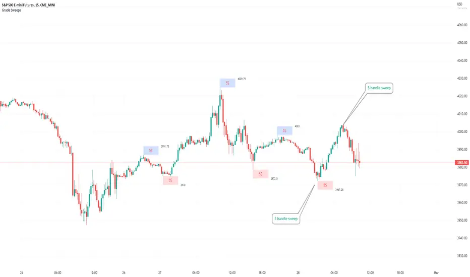
Typical Sweeps: Pivot high/low boxes. Grade sweeps, Handles/PipsTool to show typical pip-grade/ handle-grade sweep distance above pivot highs and pivot lows
-In consolidation/ranging periods (i.e. most of the time); Highs/Lows may by swept by fairly consistent distances in typical stop raids.
-Idea is from ICT teaching on typical Pip-grade sweeps in FX (10,20,30pips). Designed to work on FX, Indices, Commodities, Bitcoin.
-Above chart shows S&P; sweeping below and then above by 5 handles.
///inputs///
~choose sweep distance handles ($) or pips: will auto-calculate depending on the asset: FX= pips; Indices/stocks/commodities = handles ($)
--(2,5,10,20,30,50,100, 500, 1000)
~choose pivot lookback: larger number for more significant swing highs/lows
~choose number of historical boxes to display
~toggle on/off Pivot high boxes and Pivot low boxes independently
~extend boxes fully to the right (default is not extend)
~toggle on/off text
~text & box formatting options
Bitcoin, hourly chart; Pivot lookback = 15; $100 sweep boxes:
Eur/Usd; 15m chart; Pivot lookback = 30; 10pip sweep boxes; Boxes extended fully to the right:
Search in scripts for "text"
Peer Performance - NIFTY36STOCKSI have created a peer performance dashboard for:
36 stocks from:
5 sectors of Nifty 100
This kind of dashboard is very useful for traders when they are planing to trade in a stocks and like to see how that is stocks is performing against other stocks in the same sector . Picking outperforming stocks will always give outstanding results when market starts moving. os having view on teh complete sector will always be good for traders before picking a specific stock.
Sectors covered in this indicators are:
Indian Auto Sector
Banking Sector
Oil, Gas and Energy Stocks
Cement Sector
Technology Sector
It will help traders reviewing performance ( stock return in last 1 year) of group of stocks from a particular sector .
Basically 5 functions are used to plot this dashboard
using "if " function to shortlist the stocks and the sector it belongs to.
tablo function to plot a table with specific parameters like number of row and columns, color of the frame of table
Getting yearly return into a series of variables using "request.security" function
str.tostring function is used to convert yearly return into a series of text so that it can inserted into the table cell.
finally plotting all the text and yearly return values using table.cell function

Bodies X Wix Version of Smart Money Tools by makuchaku & eFeThis is the same Script as Super Fair Value Gaps / FVG /BoS / by makuchaku & eFe. Mine Should Default to Large Text instead of small. The Super Order Blocks I believe was meant to for you to find one of the many Smart Money tools such as turn on the Fair Value gap but leave the others off, or Turn on where the Break of Structure and leave the others off. The reason I believe this is because the default values for each of the structures were default colored (green for positive and red for negative) for all.
Mine has a different Color for every possible structure. As long as you can read with the larger text that I added, then you can create your own boxes positive for break of structure, rejection block, order blocks and fair value gaps for any time frame. The reason I did that is because There's only certain things I believe I will need to mark for myself in each time frame, and then from there You can stretch iyour own box out further in time because if price touches a fair value gap for example, the fair value gap should conyinue in time until at least 2 candles have filed the Fair valu gap going both directions. That's truly when the fair value gap should is mitigated and will from off the chart. However, If I knew How to add the code for that, I would.
Additionally, I have the Max Boxes per chart, so you should have the ability to see every OB, FVG,RJB, & BoS on the chart
I tried my hardest to create a colored border that was different from the box. But the way the original was coded was almost impossible to do. Because they defined each of the structures (FVG, OB, BoS, RJB) outer levels, when the outer levels connect via math in the code, then it joins all the outside lines for a rectangle. When creating a box, the coloe will always be the same as the border unfortunately. (Unless I replan this from the beginning)
I also Changed the default labels for reach structure from a hard to read gray to a white that pops out.
Also, chart indicators are a little large as well. Such as the cross, sideways cross, The green Triangle, and the white Diamond. You'll get used to it or you can change it as well.
Creating videos for students, you need something they can see.
So, I just wanted to ensure everything was a little more unique and easily usable when showing this to my students when I send them private videos for our weekly lessons. I'm trying to learn how to use the IPFS for THAT, (which i see has invaded PineScript) Hope this indicator helps.
If you're to borrow this, Just make sure you keep the authors in the name makuchaku & efe

ahpuhelperLibrary "ahpuhelper"
Helper Library for Auto Harmonic Patterns UltimateX. It is not meaningful for others. This is supposed to be private library. But, publishing it to make sure that I don't delete accidentally. Some functions may be useful for coders.
insert_open_trades_table_column(showOpenTrades, table_id, column, colors, values, intStatus, harmonicTrailingStartState, lblSizeOpenTrades)
add data to open trades table column
Parameters:
showOpenTrades : flag to show open trades table
table_id : Table Id
column : refers to pattern data
colors : backgroud and text color array
values : cell values
intStatus : status as integer
harmonicTrailingStartState : trailing Start state as per configs
lblSizeOpenTrades : text size
Returns: nextColumn
populate_closed_stats(ClosedStatsPosition, bullishCounts, bearishCounts, bullishRetouchCounts, bearishRetouchCounts, bullishSizeMatrix, bearishSizeMatrix, bullishRR, bearishRR, allPatternLabels, flags, rowMain, rowHeaders)
populate closed stats for harmonic patterns
Parameters:
ClosedStatsPosition : Table position for closed stats
bullishCounts : Matrix containing bullish trade stats
bearishCounts : Matrix containing bearish trade stats
bullishRetouchCounts : Matrix containing bullish trade stats for those which retouched entry
bearishRetouchCounts : Matrix containing bearish trade stats for those which retouched entry
bullishSizeMatrix : Matrix containing data about size of bullish patterns
bearishSizeMatrix : Matrix containing data about size of bearish patterns
bullishRR : Matrix containing Risk Reward data of bullish patterns
bearishRR : Matrix containing Risk Reward data of bearish patterns
allPatternLabels : array containing pattern labels
flags : display flags
rowMain : Pattern header data
rowHeaders : header grouping data
Returns: void
get_rr_details(patternTradeDetails, harmonicTrailingStartState, disableTrail, breakEvenTrail)
calculate and return risk reward based on targets and stops
Parameters:
patternTradeDetails : array containing stop, entry and targets
harmonicTrailingStartState : trailing point
disableTrail : If set, ignores trailing point
breakEvenTrail : If set, trailing does not go beyond breakeven.
Returns: nextColumn

SUPER MULTI MOVING AVERAGE [Gabbo]📈 Moving Average Indicator Update - Version 2
🔹 New Features and Improvements:
1️⃣ Enhanced MA Selection for Table Lines:
Previously, the indicator did not allow users to choose a different Moving Average type for the table lines. Now, you can select the MA type for the table.
2️⃣ New Table Text Customization Inputs:
Added inputs to choose the table text color and size for a more personalized display.
3️⃣ Improved Input Visibility and Organization:
We’ve reorganized the inputs so that the most commonly used options are now placed at the beginning for quicker and more convenient configuration.
4️⃣ Bug Fixes and Code Improvements:
Minor bugs have been fixed, and the code has been optimized for improved stability and performance. The code is now cleaner and fully functional in version 6.
5️⃣ Cometreon Public Library Integration:
To lighten the code and improve modularity, we’ve integrated the Cometreon public library. This makes the code more efficient and reduces the need to duplicate common functions.
☄️ With this update, the Moving Average indicator becomes even more versatile and user-friendly, offering a refined table interface and enhanced customization options!

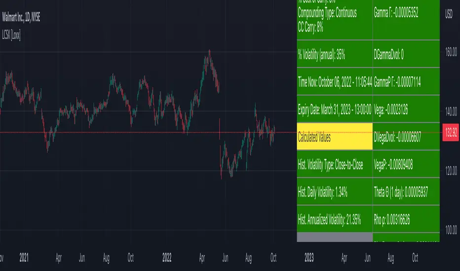
Reset Strike Options-Type 2 (Gray Whaley) [Loxx]For a reset option type 2, the strike is reset in a similar way as a reset option 1. That is, the strike is reset to the asset price at a predetermined future time, if the asset price is below (above) the initial strike price for a call (put). The payoff for such a reset call is max(S - X, 0), and max(X - S, 0) for a put, where X is equal to the original strike X if not reset, and equal to the reset strike if reset. Gray and Whaley (1999) have derived a closed-form solution for the price of European reset strike options. The price of the call option is then given by (via "The Complete Guide to Option Pricing Formulas")
c = Se^(b-r)T2 * M(a1, y1; p) - Xe^(-rT2) * M(a2, y2; p) - Se^(b-r)T1 * N(-a1) * N(z2) * e^-r(T2-T1) + Se^(b-r)T2 * N(-a1) * N(z1)
p = Se^(b-r)T1 * N(a1) * N(-z2) * e^-r(T2-T1) + Se^(b-r)T2 * N(a1) * N(-z1) + Xe^(-rT2) * M(-a2, -y2; p) - Se^(b-r)T2 * M(-a1, -y1; p)
where b is the cost-of-carry of the underlying asset, a is the volatility of the relative price changes in the asset, and r is the risk-free interest rate. K is the strike price of the option, T1 the time to reset (in years), and T2 is its time to expiration. N(x) and M(a,b; p) are, respectively, the univariate and bivariate cumulative normal distribution functions. Further
a1 = (log(S/X) + (b+v^2/2)T1) / v*T1^0.5 ... a2 = a1 - v*T1^0.5
z1 = ((b+v^2/2)(T2-T1)) / v*(T2-T1)^0.5 ... z2 = z1 - v*(T2-T1)^0.5
y1 = (log(S/X) + (b+v^2/2)T1) / v*T1^0.5 ... y2 = a1 - v*T1^0.5
and p = (T1/T2)^0.5. For reset options with multiple reset rights, see Dai, Kwok, and Wu (2003) and Liao and Wang (2003).
Inputs
Asset price ( S )
Strike price ( K )
Reset time ( T1 )
Time to maturity ( T2 )
Risk-free rate ( r )
Cost of carry ( b )
Volatility ( s )
Numerical Greeks or Greeks by Finite Difference
Analytical Greeks are the standard approach to estimating Delta, Gamma etc... That is what we typically use when we can derive from closed form solutions. Normally, these are well-defined and available in text books. Previously, we relied on closed form solutions for the call or put formulae differentiated with respect to the Black Scholes parameters. When Greeks formulae are difficult to develop or tease out, we can alternatively employ numerical Greeks - sometimes referred to finite difference approximations. A key advantage of numerical Greeks relates to their estimation independent of deriving mathematical Greeks. This could be important when we examine American options where there may not technically exist an exact closed form solution that is straightforward to work with. (via VinegarHill FinanceLabs)
Numerical Greeks Outputs
Delta D
Elasticity L
Gamma G
DGammaDvol
GammaP G
Vega
DvegaDvol
VegaP
Theta Q (1 day)
Rho r
Rho futures option r
Phi/Rho2
Carry
DDeltaDvol
Speed
Strike Delta
Strike gamma
Things to know
Only works on the daily timeframe and for the current source price.
You can adjust the text size to fit the screen

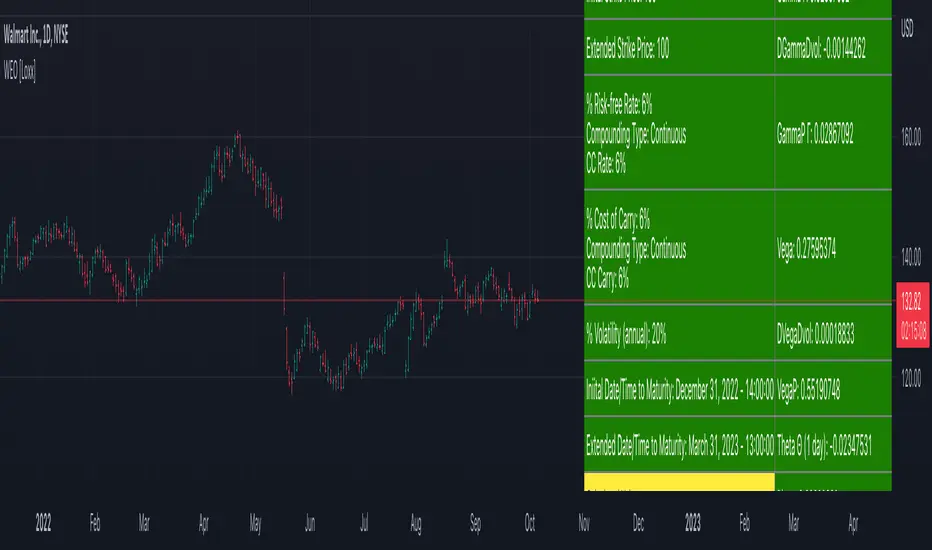
Writer Extendible Option [Loxx]These options can be exercised at their initial maturity date /I but are extended to T2 if the option is out-of-the-money at ti. The payoff from a writer-extendible call option at time T1 (T1 < T2) is (via "The Complete Guide to Option Pricing Formulas")
c(S, X1, X2, t1, T2) = (S - X1) if S>= X1 else cBSM(S, X2, T2-T1)
and for a writer-extendible put is
c(S, X1, X2, T1, T2) = (X1 - S) if S< X1 else pBSM(S, X2, T2-T1)
Writer-Extendible Call
c = cBSM(S, X1, T1) + Se^(b-r)T2 * M(Z1, -Z2; -p) - X2e^-rT2 * M(Z1 - vT^0.5, -Z2 + vT^0.5; -p)
Writer-Extendible Put
p = cBSM(S, X1, T1) + X2e^-rT2 * M(-Z1 + vT^0.5, Z2 - vT^0.5; -p) - Se^(b-r)T2 * M(-Z1, Z2; -p)
b=r options on non-dividend paying stock
b=r-q options on stock or index paying a dividend yield of q
b=0 options on futures
b=r-rf currency options (where rf is the rate in the second currency)
Inputs
Asset price ( S )
Initial strike price ( X1 )
Extended strike price ( X2 )
Initial time to maturity ( t1 )
Extended time to maturity ( T2 )
Risk-free rate ( r )
Cost of carry ( b )
Volatility ( s )
Numerical Greeks or Greeks by Finite Difference
Analytical Greeks are the standard approach to estimating Delta, Gamma etc... That is what we typically use when we can derive from closed form solutions. Normally, these are well-defined and available in text books. Previously, we relied on closed form solutions for the call or put formulae differentiated with respect to the Black Scholes parameters. When Greeks formulae are difficult to develop or tease out, we can alternatively employ numerical Greeks - sometimes referred to finite difference approximations. A key advantage of numerical Greeks relates to their estimation independent of deriving mathematical Greeks. This could be important when we examine American options where there may not technically exist an exact closed form solution that is straightforward to work with. (via VinegarHill FinanceLabs)
Numerical Greeks Output
Delta
Elasticity
Gamma
DGammaDvol
GammaP
Vega
DvegaDvol
VegaP
Theta (1 day)
Rho
Rho futures option
Phi/Rho2
Carry
DDeltaDvol
Speed
Things to know
Only works on the daily timeframe and for the current source price.
You can adjust the text size to fit the screen
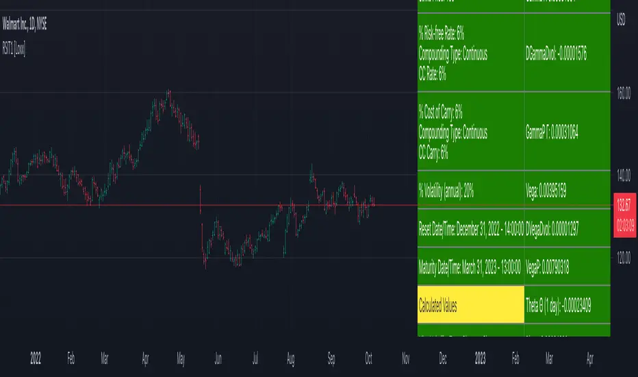
Reset Strike Options-Type 1 [Loxx]In a reset call (put) option, the strike is reset to the asset price at a predetermined future time, if the asset price is below (above) the initial strike price. This makes the strike path-dependent. The payoff for a call at maturity is equal to max((S-X)/X, 0) where is equal to the original strike X if not reset, and equal to the reset strike if reset. Similarly, for a put, the payoff is max((X-S)/X, 0) Gray and Whaley (1997) x have derived a closed-form solution for such an option. For a call, we have
c = e^(b-r)(T2-T1) * N(-a2) * N(z1) * e^(-rt1) - e^(-rT2) * N(-a2)*N(z2) - e^(-rT2) * M(a2, y2; p) + (S/X) * e^(b-r)T2 * M(a1, y1; p)
and for a put,
p = e^(-rT2) * N(a2) * N(-z2) - e^(b-r)(T2-T1) * N(a2) * N(-z1) * e^(-rT1) + e^(-rT2) * M(-a2, -y2; p) - (S/X) * e^(b-r)T2 * M(-a1, -y1; p)
where b is the cost-of-carry of the underlying asset, a is the volatil- ity of the relative price changes in the asset, and r is the risk-free interest rate. X is the strike price of the option, r the time to reset (in years), and T is its time to expiration. N(x) and M(a, b; p) are, respec- tively, the univariate and bivariate cumulative normal distribution functions. The remaining parameters are p = (T1/T2)^0.5 and
a1 = (log(S/X) + (b+v^2/2)T1) / vT1^0.5 ... a2 = a1 - vT1^0.5
z1 = (b+v^2/2)(T2-T1)/v(T2-T1)^0.5 ... z2 = z1 - v(T2-T1)^0.5
y1 = log(S/X) + (b+v^2)T2 / vT2^0.5 ... y2 = y1 - vT2^0.5
b=r options on non-dividend paying stock
b=r-q options on stock or index paying a dividend yield of q
b=0 options on futures
b=r-rf currency options (where rf is the rate in the second currency)
Inputs
Asset price ( S )
Initial strike price ( X1 )
Extended strike price ( X2 )
Initial time to maturity ( t1 )
Extended time to maturity ( T2 )
Risk-free rate ( r )
Cost of carry ( b )
Volatility ( s )
Numerical Greeks or Greeks by Finite Difference
Analytical Greeks are the standard approach to estimating Delta, Gamma etc... That is what we typically use when we can derive from closed form solutions. Normally, these are well-defined and available in text books. Previously, we relied on closed form solutions for the call or put formulae differentiated with respect to the Black Scholes parameters. When Greeks formulae are difficult to develop or tease out, we can alternatively employ numerical Greeks - sometimes referred to finite difference approximations. A key advantage of numerical Greeks relates to their estimation independent of deriving mathematical Greeks. This could be important when we examine American options where there may not technically exist an exact closed form solution that is straightforward to work with. (via VinegarHill FinanceLabs)
Numerical Greeks Ouput
Delta
Elasticity
Gamma
DGammaDvol
GammaP
Vega
DvegaDvol
VegaP
Theta (1 day)
Rho
Rho futures option
Phi/Rho2
Carry
DDeltaDvol
Speed
Things to know
Only works on the daily timeframe and for the current source price.
You can adjust the text size to fit the screen
Fade-in Options [Loxx]A fade-in call has the same payoff as a standard call except the size of the payoff is weighted by how many fixings the asset price were inside a predefined range (L, U). If the asset price is inside the range for every fixing, the payoff will be identical to a plain vanilla option. More precisely, for a call option, the payoff will be max(S(T) - X, 0) X 1/n Sum(n(i)), where n is the total number of fixings and n(i) = 1 if at fixing i the asset price is inside the range, and n(i) = 0 otherwise. Similarly, for a put, the payoff is max(X - S(T), 0) X 1/n Sum(n(i)).
Brockhaus, Ferraris, Gallus, Long, Martin, and Overhaus (1999) describe a closed-form formula for fade-in options. For a call the value is given by
max(X - S(T), 0) X 1/n Sum(n(i))
describe a closed-form formula for fade-in options. For a call the value is given by
c = 1/n * Sum(S^((b-r)*T) * (M(-d5, d1; -p) - M(-d3, d1; -p)) - Xe^(-rT) * (M(-d6, d2; -p) - M(-d4, d2; -p))
where n is the number of fixings, p = (t1^0.5/T^0.5), t1 = iT/n
d1 = (log(S/X) + (b + v^2/2)*T) / (v * T^0.5) ... d2 = d1 - v*T^0.5
d3 = (log(S/L) + (b + v^2/2)*t1) / (v * t1^0.5) ... d4 = d3 - v*t1^0.5
d5 = (log(S/U) + (b + v^2/2)*t1) / (v * t1^0.5) ... d6 = d5 - v*t1^0.5
The value of a put is similarly
p = 1/n * Sum(Xe^(-rT) * (M(-d6, -d2; -p) - M(-d4, -d2; -p))) - S^((b-r)*T) * (M(-d5, -d1; -p) - M(-d3, -d1; -p)
b=r options on non-dividend paying stock
b=r-q options on stock or index paying a dividend yield of q
b=0 options on futures
b=r-rf currency options (where rf is the rate in the second currency)
Inputs
Asset price ( S )
Strike price ( K )
Lower barrier ( L )
Upper barrier ( U )
Time to maturity ( T )
Risk-free rate ( r )
Cost of carry ( b )
Volatility ( s )
Fixings ( n )
cnd1(x) = Cumulative Normal Distribution
nd(x) = Standard Normal Density Function
cbnd3() = Cumulative Bivariate Distribution
convertingToCCRate(r, cmp ) = Rate compounder
Numerical Greeks or Greeks by Finite Difference
Analytical Greeks are the standard approach to estimating Delta, Gamma etc... That is what we typically use when we can derive from closed form solutions. Normally, these are well-defined and available in text books. Previously, we relied on closed form solutions for the call or put formulae differentiated with respect to the Black Scholes parameters. When Greeks formulae are difficult to develop or tease out, we can alternatively employ numerical Greeks - sometimes referred to finite difference approximations. A key advantage of numerical Greeks relates to their estimation independent of deriving mathematical Greeks. This could be important when we examine American options where there may not technically exist an exact closed form solution that is straightforward to work with. (via VinegarHill FinanceLabs)
Things to know
Only works on the daily timeframe and for the current source price.
You can adjust the text size to fit the screen

Log Contract Ln(S/X) [Loxx]A log contract, first introduced by Neuberger (1994) and Neuberger (1996), is not strictly an option. It is, however, an important building block in volatility derivatives (see Chapter 6 as well as Demeterfi, Derman, Kamal, and Zou, 1999). The payoff from a log contract at maturity T is simply the natural logarithm of the underlying asset divided by the strike price, ln(S/ X). The payoff is thus nonlinear and has many similarities with options. The value of this contract is (via "The Complete Guide to Option Pricing Formulas")
L = e^(-r * T) * (log(S/X) + (b-v^2/2)*T)
The delta of a log contract is
delta = (e^(-r*T) / S)
and the gamma is
gamma = (e^(-r*T) / S^2)
Inputs
S = Stock price.
K = Strike price of option.
T = Time to expiration in years.
r = Risk-free rate
c = Cost of Carry
V = Variance of the underlying asset price
cnd1(x) = Cumulative Normal Distribution
nd(x) = Standard Normal Density Function
convertingToCCRate(r, cmp ) = Rate compounder
Numerical Greeks or Greeks by Finite Difference
Analytical Greeks are the standard approach to estimating Delta, Gamma etc... That is what we typically use when we can derive from closed form solutions. Normally, these are well-defined and available in text books. Previously, we relied on closed form solutions for the call or put formulae differentiated with respect to the Black Scholes parameters. When Greeks formulae are difficult to develop or tease out, we can alternatively employ numerical Greeks - sometimes referred to finite difference approximations. A key advantage of numerical Greeks relates to their estimation independent of deriving mathematical Greeks. This could be important when we examine American options where there may not technically exist an exact closed form solution that is straightforward to work with. (via VinegarHill FinanceLabs)
Things to know
Only works on the daily timeframe and for the current source price.
You can adjust the text size to fit the screen
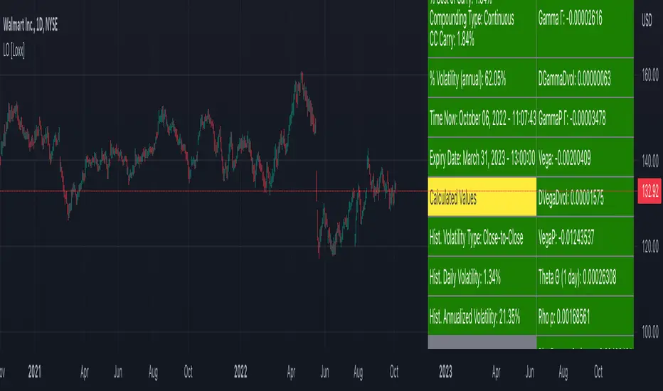
Log Option [Loxx]A log option introduced by Wilmott (2000) has a payoff at maturity equal to max(log(S/X), 0), which is basically an option on the rate of return on the underlying asset with strike log(X). The value of a log option is given by: (via "The Complete Guide to Option Pricing Formulas")
e^−rT * n(d2)σ√(T − t) + e^−rT*(log(S/K) + (b −σ^2/2)T) * N(d2)
where N(*) is the cumulative normal distribution function, n(*) is the normal density function, and
d = ((log(S/X) + (b - v^2/2)*T) / (v*T^0.5)
b=r options on non-dividend paying stock
b=r-q options on stock or index paying a dividend yield of q
b=0 options on futures
b=r-rf currency options (where rf is the rate in the second currency)
Inputs
S = Stock price.
K = Strike price of option.
T = Time to expiration in years.
r = Risk-free rate
c = Cost of Carry
V = Variance of the underlying asset price
cnd1(x) = Cumulative Normal Distribution
nd(x) = Standard Normal Density Function
convertingToCCRate(r, cmp ) = Rate compounder
Numerical Greeks or Greeks by Finite Difference
Analytical Greeks are the standard approach to estimating Delta, Gamma etc... That is what we typically use when we can derive from closed form solutions. Normally, these are well-defined and available in text books. Previously, we relied on closed form solutions for the call or put formulae differentiated with respect to the Black Scholes parameters. When Greeks formulae are difficult to develop or tease out, we can alternatively employ numerical Greeks - sometimes referred to finite difference approximations. A key advantage of numerical Greeks relates to their estimation independent of deriving mathematical Greeks. This could be important when we examine American options where there may not technically exist an exact closed form solution that is straightforward to work with. (via VinegarHill FinanceLabs)
Things to know
Only works on the daily timeframe and for the current source price.
You can adjust the text size to fit the screen
Log Contract Ln(S) [Loxx]A log contract, first introduced by Neuberger (1994) and Neuberger (1996), is not strictly an option. It is, however, an important building block in volatility derivatives (see Chapter 6 as well as Demeterfi, Derman, Kamal, and Zou, 1999). The payoff from a log contract at maturity T is simply the natural logarithm of the underlying asset divided by the strike price, ln(S/ X). The payoff is thus nonlinear and has many similarities with options. The value of this contract is (via "The Complete Guide to Option Pricing Formulas")
L = e^(-r * T) * (log(S/X) + (b-v^2/2)*T)
The delta of a log contract is
delta = (e^(-r*T) / S)
and the gamma is
gamma = (e^(-r*T) / S^2)
An even simpler version of the log contract is when the payoff simply is ln(S). The payoff is clearly still nonlinear in the underlying asset. It follows that the value of this contract is:
L = e^(-r * T) * (log(S) + (b-v^2/2)*T)
The theta/time decay of a log contract is
theta = - 1/T * v^2
and its exposure to the stock price, delta, is
delta = - 2/T * 1/S
This basically tells you that you need to be long stocks to be delta- neutral at any time. Moreover, the gamma is
gamma = 2 / (T * S^2)
b=r options on non-dividend paying stock
b=r-q options on stock or index paying a dividend yield of q
b=0 options on futures
b=r-rf currency options (where rf is the rate in the second currency)
Inputs
S = Stock price.
T = Time to expiration in years.
r = Risk-free rate
c = Cost of Carry
V = volatility of the underlying asset price
cnd1(x) = Cumulative Normal Distribution
nd(x) = Standard Normal Density Function
convertingToCCRate(r, cmp ) = Rate compounder
Numerical Greeks or Greeks by Finite Difference
Analytical Greeks are the standard approach to estimating Delta, Gamma etc... That is what we typically use when we can derive from closed form solutions. Normally, these are well-defined and available in text books. Previously, we relied on closed form solutions for the call or put formulae differentiated with respect to the Black Scholes parameters. When Greeks formulae are difficult to develop or tease out, we can alternatively employ numerical Greeks - sometimes referred to finite difference approximations. A key advantage of numerical Greeks relates to their estimation independent of deriving mathematical Greeks. This could be important when we examine American options where there may not technically exist an exact closed form solution that is straightforward to work with. (via VinegarHill FinanceLabs)
Things to know
Only works on the daily timeframe and for the current source price.
You can adjust the text size to fit the screen

Powered Option [Loxx]At maturity, a powered call option pays off max(S - X, 0)^i and a put pays off max(X - S, 0)^i . Esser (2003 describes how to value these options (see also Jarrow and Turnbull, 1996, Brockhaus, Ferraris, Gallus, Long, Martin, and Overhaus, 1999). (via "The Complete Guide to Option Pricing Formulas")
b=r options on non-dividend paying stock
b=r-q options on stock or index paying a dividend yield of q
b=0 options on futures
b=r-rf currency options (where rf is the rate in the second currency)
Inputs
S = Stock price.
K = Strike price of option.
T = Time to expiration in years.
r = Risk-free rate
c = Cost of Carry
V = volatility of the underlying asset price
i = power
cnd1(x) = Cumulative Normal Distribution
nd(x) = Standard Normal Density Function
combin(x) = Combination function, calculates the number of possible combinations for two given numbers
convertingToCCRate(r, cmp ) = Rate compounder
Numerical Greeks or Greeks by Finite Difference
Analytical Greeks are the standard approach to estimating Delta, Gamma etc... That is what we typically use when we can derive from closed form solutions. Normally, these are well-defined and available in text books. Previously, we relied on closed form solutions for the call or put formulae differentiated with respect to the Black Scholes parameters. When Greeks formulae are difficult to develop or tease out, we can alternatively employ numerical Greeks - sometimes referred to finite difference approximations. A key advantage of numerical Greeks relates to their estimation independent of deriving mathematical Greeks. This could be important when we examine American options where there may not technically exist an exact closed form solution that is straightforward to work with. (via VinegarHill FinanceLabs)
Things to know
Only works on the daily timeframe and for the current source price.
You can adjust the text size to fit the screen

Capped Standard Power Option [Loxx]Power options can lead to very high leverage and thus entail potentially very large losses for short positions in these options. It is therefore common to cap the payoff. The maximum payoff is set to some predefined level C. The payoff at maturity for a capped power call is min . Esser (2003) gives the closed-form solution: (via "The Complete Guide to Option Pricing Formulas")
c = S^i * (e^((i - 1) * (r + i*v^2 / 2) - i * (r - b))*T) * (N(e1) - N(e3)) - e^(-r*T) * (X*N(e2) - (C + X) * N(e4))
while the value of a put is
e1 = (log(S/X^(1/i)) + (b + (i - 1/2)*v^2)*T) / v*T^0.5
e3 = (log(S/(C + X)^(1/i)) + (b + (i - 1/2)*v^2)*T) / v*T^0.5
e4 = e3 - i * v * T^0.5
In the case of a capped power put, we have
p = e^(-r*T) * (X*N(-e2) - (C + X) * N(-e4)) - S^i * (e^((i - 1) * (r + i*v^2 / 2) - i * (r - b))*T) * (N(-e1) - N(-e3))
where e1 and e2 is as before. e3 and e4 has to be changed to
e3 = (log(S/(X - C)^(1/i)) + (b + (i - 1/2)*v^2)*T) / v*T^0.5
e4 = e3 - i * v * T^0.5
b=r options on non-dividend paying stock
b=r-q options on stock or index paying a dividend yield of q
b=0 options on futures
b=r-rf currency options (where rf is the rate in the second currency)
Inputs
S = Stock price.
K = Strike price of option.
T = Time to expiration in years.
r = Risk-free rate
c = Cost of Carry
V = Variance of the underlying asset price
i = power
c = Capped on pay off
cnd1(x) = Cumulative Normal Distribution
nd(x) = Standard Normal Density Function
convertingToCCRate(r, cmp ) = Rate compounder
Numerical Greeks or Greeks by Finite Difference
Analytical Greeks are the standard approach to estimating Delta, Gamma etc... That is what we typically use when we can derive from closed form solutions. Normally, these are well-defined and available in text books. Previously, we relied on closed form solutions for the call or put formulae differentiated with respect to the Black Scholes parameters. When Greeks formulae are difficult to develop or tease out, we can alternatively employ numerical Greeks - sometimes referred to finite difference approximations. A key advantage of numerical Greeks relates to their estimation independent of deriving mathematical Greeks. This could be important when we examine American options where there may not technically exist an exact closed form solution that is straightforward to work with. (via VinegarHill FinanceLabs)
Things to know
Only works on the daily timeframe and for the current source price.
You can adjust the text size to fit the screen

Standard Power Option [Loxx]Standard power options (aka asymmetric power options) have nonlinear payoff at maturity. For a call, the payoff is max(S^i - X, 0), and for a put, it is max(X - S^i , 0), where i is some power (i > 0). The value of this power call is given by (see Heynen and Kat, 1996c; Zhang, 1998; and Esser, 2003). (via "The Complete Guide to Option Pricing Formulas")
c = S^i * (e^((i - 1) * (r + i*v^2 / 2) - i * (r - b))*T) * N(d1) - X*e^(-r*T) * N(d2)
while the value of a put is
p = X*e^(-r*T) * N(-d2) - S^i * (e^((i - 1) * (r + i*v^2 / 2) - i * (r - b))*T) * N(-d1)
where
d1 = (log(S/X^(1/i)) + (b + (i - 1/2)*v^2)*T) / v*T^0.5
d2 = d1 - i * v * T^0.5
b=r options on non-dividend paying stock
b=r-q options on stock or index paying a dividend yield of q
b=0 options on futures
b=r-rf currency options (where rf is the rate in the second currency)
Inputs
S = Stock price.
K = Strike price of option.
T = Time to expiration in years.
r = Risk-free rate
c = Cost of Carry
V = Variance of the underlying asset price
pwr = power
cnd1(x) = Cumulative Normal Distribution
nd(x) = Standard Normal Density Function
convertingToCCRate(r, cmp ) = Rate compounder
Numerical Greeks or Greeks by Finite Difference
Analytical Greeks are the standard approach to estimating Delta, Gamma etc... That is what we typically use when we can derive from closed form solutions. Normally, these are well-defined and available in text books. Previously, we relied on closed form solutions for the call or put formulae differentiated with respect to the Black Scholes parameters. When Greeks formulae are difficult to develop or tease out, we can alternatively employ numerical Greeks - sometimes referred to finite difference approximations. A key advantage of numerical Greeks relates to their estimation independent of deriving mathematical Greeks. This could be important when we examine American options where there may not technically exist an exact closed form solution that is straightforward to work with. (via VinegarHill FinanceLabs)
Things to know
Only works on the daily timeframe and for the current source price.
You can adjust the text size to fit the screen

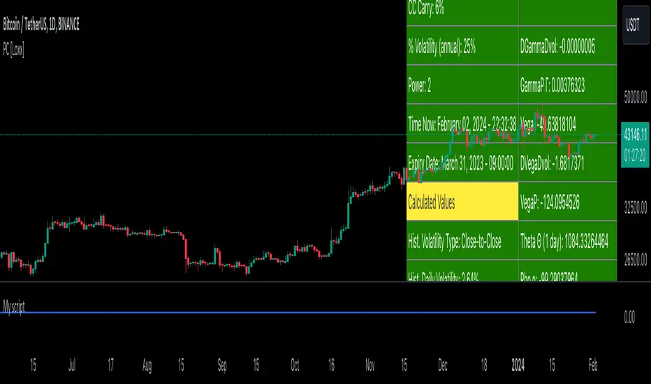
Power Contract [Loxx]There are two main categories of power options. Standard power options' payoff depends on the price of the underlying asset raised to some power. For powered options, the "standard" payoff (stock price in excess of the exercise price) is raised to some power.
A power contract is a simple derivative instrument paying (S/ X)^i at maturity, where i is some fixed power. The value of such a power contract is given by Shaw (1998) as: (via "The Complete Guide to Option Pricing Formulas")
VPower = (S/X)^i * e^((b-v^2)/2)*i - r + i^2 * v^2/2)*T
b=r options on non-dividend paying stock
b=r-q options on stock or index paying a dividend yield of q
b=0 options on futures
b=r-rf currency options (where rf is the rate in the second currency)
Inputs
S = Stock price.
K = Strike price of option.
T = Time to expiration in years.
r = Risk-free rate
c = Cost of Carry
V = Variance of the underlying asset price
lambda = Jump rate per year
cnd1(x) = Cumulative Normal Distribution
nd(x) = Standard Normal Density Function
convertingToCCRate(r, cmp ) = Rate compounder
Numerical Greeks or Greeks by Finite Difference
Analytical Greeks are the standard approach to estimating Delta, Gamma etc... That is what we typically use when we can derive from closed form solutions. Normally, these are well-defined and available in text books. Previously, we relied on closed form solutions for the call or put formulae differentiated with respect to the Black Scholes parameters. When Greeks formulae are difficult to develop or tease out, we can alternatively employ numerical Greeks - sometimes referred to finite difference approximations. A key advantage of numerical Greeks relates to their estimation independent of deriving mathematical Greeks. This could be important when we examine American options where there may not technically exist an exact closed form solution that is straightforward to work with. (via VinegarHill FinanceLabs)
Things to know
Only works on the daily timeframe and for the current source price.
You can adjust the text size to fit the screen
Daily VolumeShows a table in the top right of the chart with a few options:
Only show intraday: By default the table will not be visible on timeframes of 1D or above, but this can be changed to show all the time if desired.
Daily volume: Displays the volume for the day so far, regardless of what timeframe is currently showing.
Yesterday's volume: Displays the volume from the previous day. As with the daily volume , it will show the entire previous day's volume regardless of the current timeframe.
Average Volume: Displays the average volume based on a user-specified number of days. The default value is 30 days.
Text color and table color: Choose the color settings for the table text and background.

Moneyness Options [Loxx]A moneyness option is basically a plain vanilla option where the strike is set to a percentage of the future/forward price. For example, a 120% moneyness call would have a strike equal to 120% of the forward price. A 120% moneyness put would have a spot equal to 120% of the strike. The value of this option is given in percent of the forward. The value of a moneyness call or put is thus given by: (via "The Complete Guide to Option Pricing Formulas")
c = p = c^-rT * (N(d1) - LN(d2))
where L = X/F for a call and L = F/X for a put, and
d1 = (-log(L) + v^2*T/2) / (v*T^0.5)
d2 = d1 - (v*T^0.5)
b=r options on non-dividend paying stock
b=r-q options on stock or index paying a dividend yield of q
b=0 options on futures
b=r-rf currency options (where rf is the rate in the second currency)
Inputs
S = Stock price.
K = Strike price of option.
T = Time to expiration in years.
r = Risk-free rate
c = Cost of Carry
V = Variance of the underlying asset price
lambda = Jump rate per year
cnd1(x) = Cumulative Normal Distribution
nd(x) = Standard Normal Density Function
convertingToCCRate(r, cmp ) = Rate compounder
Numerical Greeks or Greeks by Finite Difference
Analytical Greeks are the standard approach to estimating Delta, Gamma etc... That is what we typically use when we can derive from closed form solutions. Normally, these are well-defined and available in text books. Previously, we relied on closed form solutions for the call or put formulae differentiated with respect to the Black Scholes parameters. When Greeks formulae are difficult to develop or tease out, we can alternatively employ numerical Greeks - sometimes referred to finite difference approximations. A key advantage of numerical Greeks relates to their estimation independent of deriving mathematical Greeks. This could be important when we examine American options where there may not technically exist an exact closed form solution that is straightforward to work with. (via VinegarHill FinanceLabs)
Things to know
Only works on the daily timeframe and for the current source price.
You can adjust the text size to fit the screen

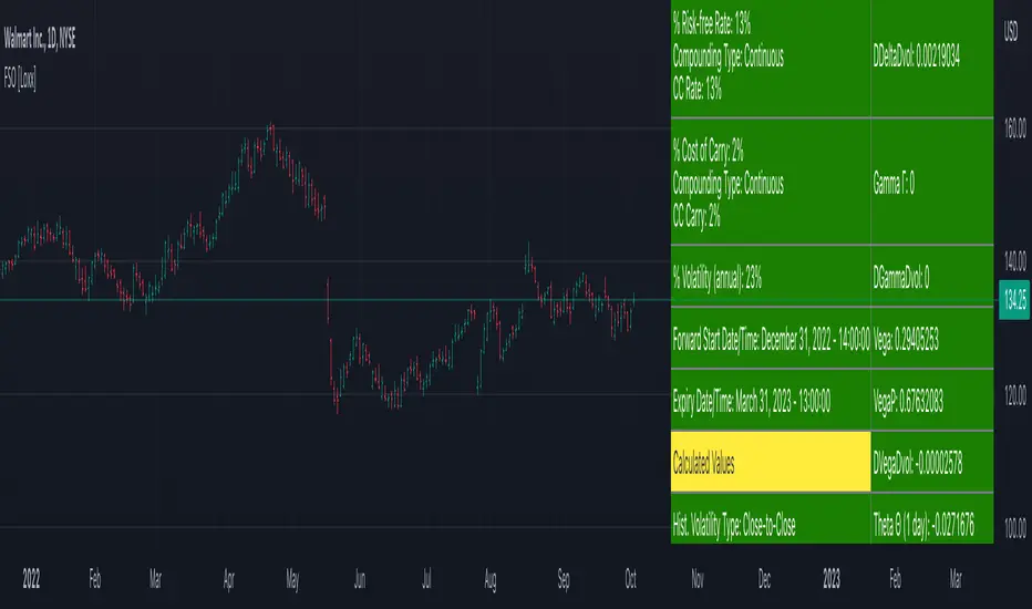
Forward Start Options [Loxx]A forward start option with time to maturity T starts at-the-money or proportionally in- or out-of-the-money after a known elapsed time t in the future. The strike is set equal to a positive constant a times the asset price S after the known time t. If a is less than unity, the call (put) will start 1 - a percent in-the-money (out-of-the- money); if a is unity, the option will start at-the-money; and if a is larger than unity, the call (put) will start a - 1 percentage out-of-the- money (in-the-money).A forward start option can be priced using the Rubinstein (1990) formula: (via "The Complete Guide to Option Pricing Formulas")
c = S*e^(b-r)t * (e^(b-r)(T-t) * N(d1)) - alpha * e^-r(T-t) * N(d2))
p = S*e^(b-r)t * (alpha*e^r(T-t) * N(-d2)) - e^-(b-r)(T-t) * N(-d1))
where
d1 = (log(1/alpha) + (b + v^2/2)(T-1))/v*(T-t)^0.5
d2 = d1 - v*(T-t)^0.5
Application
Employee options are often of the forward starting type. Ratchet options (aka cliquet options) consist of a series of forward starting options.
b=r options on non-dividend paying stock
b=r-q options on stock or index paying a dividend yield of q
b=0 options on futures
b=r-rf currency options (where rf is the rate in the second currency)
Inputs
S = Stock price.
a = Alpha
T1 = Time to forward start
T = Time to expiration in years.
r = Risk-free rate
c = Cost of Carry
v = volatility of the underlying asset price
Numerical Greeks or Greeks by Finite Difference
Analytical Greeks are the standard approach to estimating Delta, Gamma etc... That is what we typically use when we can derive from closed form solutions. Normally, these are well-defined and available in text books. Previously, we relied on closed form solutions for the call or put formulae differentiated with respect to the Black Scholes parameters. When Greeks formulae are difficult to develop or tease out, we can alternatively employ numerical Greeks - sometimes referred to finite difference approximations. A key advantage of numerical Greeks relates to their estimation independent of deriving mathematical Greeks. This could be important when we examine American options where there may not technically exist an exact closed form solution that is straightforward to work with. (via VinegarHill FinanceLabs)
Things to know
Only works on the daily timeframe and for the current source price.
You can adjust the text size to fit the screen
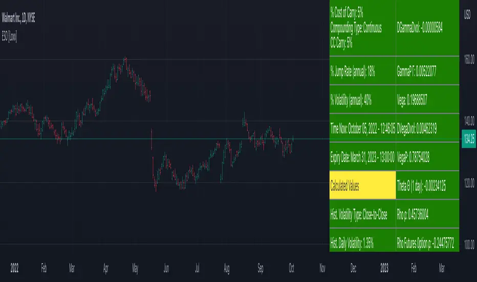
Executive Stock Options [Loxx]The Jennergren and Naslund (1993) formula takes into account that an employee or executive often loses her options if she has to leave the company before the option's expiration: (via "The Complete Guide to Option Pricing Formulas")
c = e^(-lambda*T) * (Se^((b-r)T) * N(d1) - Xe^-rT * N(d2))
p = e^(-lambda*T) * (Xe^(-rT) * N(-d2) - Se^(b-r)T * N(-d1))
where
d1 = (log(S/X) + (b + v^2/2)T) / vT^0.5
d2 = d1 - vT^0.5
lambda is the jump rate per year. The value of the executive option equals the ordinary Black-Scholes option price multiplied by the probability e —AT that the executive will stay with the firm until the option expires.
b=r options on non-dividend paying stock
b=r-q options on stock or index paying a dividend yield of q
b=0 options on futures
b=r-rf currency options (where rf is the rate in the second currency)
Inputs
S = Stock price.
K = Strike price of option.
T = Time to expiration in years.
r = Risk-free rate
c = Cost of Carry
V = Variance of the underlying asset price
lambda = Jump rate per year
cnd1(x) = Cumulative Normal Distribution
nd(x) = Standard Normal Density Function
convertingToCCRate(r, cmp ) = Rate compounder
Numerical Greeks or Greeks by Finite Difference
Analytical Greeks are the standard approach to estimating Delta, Gamma etc... That is what we typically use when we can derive from closed form solutions. Normally, these are well-defined and available in text books. Previously, we relied on closed form solutions for the call or put formulae differentiated with respect to the Black Scholes parameters. When Greeks formulae are difficult to develop or tease out, we can alternatively employ numerical Greeks - sometimes referred to finite difference approximations. A key advantage of numerical Greeks relates to their estimation independent of deriving mathematical Greeks. This could be important when we examine American options where there may not technically exist an exact closed form solution that is straightforward to work with. (via VinegarHill FinanceLabs)
Things to know
Only works on the daily timeframe and for the current source price.
You can adjust the text size to fit the screen
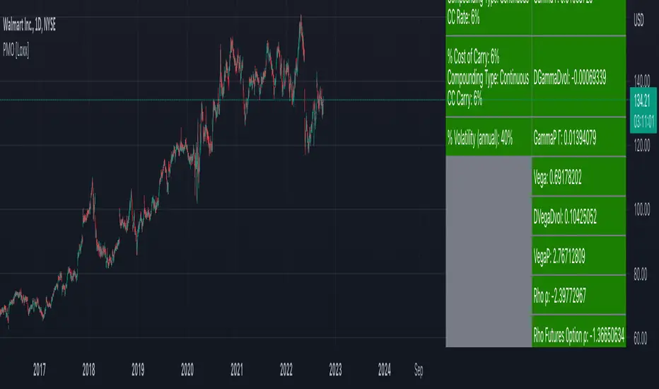
Perpetual American Options [Loxx]Perpetual American Options is Perpetual American Options pricing model. This indicator also includes numerical greeks.
American Perpetual Options
While there in general is no closed-form solution for American options (except for non-dividend-paying stock call options) it is possible to find a closed-form solution for options with an infinite time to expiration. The reason is that the time to expiration will always be the same: infinite. The time to maturity, therefore, does not depend on at what point in time we look at the valuation problem, which makes the valuation problem independent of time McKean (1965) and Merton (1973) gives closed-form solutions for American perpetual options. For a call option we have
c = (X / (y1 - 1)) * ((y1 - 1)/y1 * S/X)^y1
where
y1 = 1/2 - b/v^2 + ((b/v^2 - 1/2)^2 + 2*r/v^2)^0.5
If b >= r, then there is never optimal to exercise a call option. In the case of an American perpetual put, we have
p = X/(1-y2) * (((y2 - 1) / y2) * S/X)^y2
where
y2 = 1/2 - b/v^2 - ((b/v^2 - 1/2)^2 + 2*r/v^2)^0.5
In practice, one can naturally discuss if there is such a thing as infinite time to maturity. For instance, credit risk could play an important role: Even when you are buying an option from an AAA bank, there is no guarantee the bank will be around forever.
b=r options on non-dividend paying stock
b=r-q options on stock or index paying a dividend yield of q
b=0 options on futures
b=r-rf currency options (where rf is the rate in the second currency)
Inputs
S = Stock price.
K = Strike price of option.
T = Time to expiration in years.
r = Risk-free rate
c = Cost of Carry
V = Variance of the underlying asset price
cnd1(x) = Cumulative Normal Distribution
cbnd3(x) = Cumulative Bivariate Normal Distribution
nd(x) = Standard Normal Density Function
convertingToCCRate(r, cmp ) = Rate compounder
Numerical Greeks or Greeks by Finite Difference
Analytical Greeks are the standard approach to estimating Delta, Gamma etc... That is what we typically use when we can derive from closed form solutions. Normally, these are well-defined and available in text books. Previously, we relied on closed form solutions for the call or put formulae differentiated with respect to the Black Scholes parameters. When Greeks formulae are difficult to develop or tease out, we can alternatively employ numerical Greeks - sometimes referred to finite difference approximations. A key advantage of numerical Greeks relates to their estimation independent of deriving mathematical Greeks. This could be important when we examine American options where there may not technically exist an exact closed form solution that is straightforward to work with. (via VinegarHill FinanceLabs)
Things to know
Only works on the daily timeframe and for the current source price.
You can adjust the text size to fit the screen
American Approximation Bjerksund & Stensland 2002 [Loxx]American Approximation Bjerksund & Stensland 2002 is an American Options pricing model. This indicator also includes numerical greeks. You can compare the output of the American Approximation to the Black-Scholes-Merton value on the output of the options panel.
The Bjerksund & Stensland (2002) Approximation
The Bjerksund and Stensland (2002) approximation divides the time to maturity into two parts, each with a separate flat exercise boundary. It is thus a straightforward generalization of the Bjerksund-Stensland 1993 algorithm. The method is fast and efficient and should be more accurate than the Barone-Adesi and Whaley (1987) and the Bjerksund and Stensland (1993b) approximations. The algorithm requires an accurate cumulative bivariate normal approximation. Several approximations that are described in the literature are not sufficiently accurate, but the Genze algorithm works.
C = alpha2*S^B - alpha2*phi(S, t1, B, I2, I2)
+ phi(S, t1, I2, I2) - phi(S, t1, I, I1, I2)
- X*phi(S, t1, 0, I2, I2) + X*phi(S, t1, 0, I1, I2)
+ alpha1*phi(X, t1, B, I1, I2) - alpha1*psi*St, T, B, I1, I2, I1, t1)
+ psi(S, T, 1, I1, I2, I1, t1) - psi(S, T, 1, X, I2, I1, t1)
- X*psi(S, T, 0, I1, I2, I1, t1) + psi(S, T, 0 ,X, I2, I1, t1)
where
alpha1 = (I1 - X)*I1^-B
alpha2 = (I2 - X)*I2^-B
B = (1/2 - b/v^2) + ((b/v^2 - 1/2)^2 + 2*(r/v^2))^0.5
The function psi(S, T, y, H, I) is given by
psi(S, T, gamma, H, I) = e^lambda * S^gamma * (N(-d) - (I/S)^k * N(-d2))
d = (log(S/H) + (b + (gamma - 1/2) * v^2) * T) / (v * T^0.5)
d2 = (log(I^2/(S*H)) + (b + (gamma - 1/2) * v^2) * T) / (v * T^0.5)
lambda = -r + gamma * b + 1/2 * gamma * (gamma - 1) * v^2
k = 2*b/v^2 + (2 * gamma - 1)
and the trigger price I is defined as
I1 = B0 + (B(+infi) - B0) * (1 - e^h1)
I2 = B0 + (B(+infi) - B0) * (1 - e^h2)
h1 = -(b*t1 + 2*v*t1^0.5) * (X^2 / ((B(+infi) - B0))*B0)
h2 = -(b*T + 2*v*T^0.5) * (X^2 / ((B(+infi) - B0))*B0)
t1 = 1/2 * (5^0.5 - 1) * T
B(+infi) = (B / (B - 1)) * X
B0 = max(X, (r / (r - b)) * X)
Moreover, the function psi(S, T, gamma, H, I2, I1, t1) is given by
psi(S, T, gamma, H, I2, I1, t1, r, b, v) = e^(lambda * T) * S^gamma * (M(-e1, -f1, rho) - (I2/S)^k * M(-e2, -f2, rho)
- (I1/S)^k * M(-e3, -f3, -rho) + (I1/I2)^k * M(-e4, -f4, -rho))
where (see screenshot for e and f values)
b=r options on non-dividend paying stock
b=r-q options on stock or index paying a dividend yield of q
b=0 options on futures
b=r-rf currency options (where rf is the rate in the second currency)
Inputs
S = Stock price.
K = Strike price of option.
T = Time to expiration in years.
r = Risk-free rate
c = Cost of Carry
V = Variance of the underlying asset price
cnd1(x) = Cumulative Normal Distribution
cbnd3(x) = Cumulative Bivariate Normal Distribution
nd(x) = Standard Normal Density Function
convertingToCCRate(r, cmp ) = Rate compounder
Numerical Greeks or Greeks by Finite Difference
Analytical Greeks are the standard approach to estimating Delta, Gamma etc... That is what we typically use when we can derive from closed form solutions. Normally, these are well-defined and available in text books. Previously, we relied on closed form solutions for the call or put formulae differentiated with respect to the Black Scholes parameters. When Greeks formulae are difficult to develop or tease out, we can alternatively employ numerical Greeks - sometimes referred to finite difference approximations. A key advantage of numerical Greeks relates to their estimation independent of deriving mathematical Greeks. This could be important when we examine American options where there may not technically exist an exact closed form solution that is straightforward to work with. (via VinegarHill FinanceLabs)
Things to know
Only works on the daily timeframe and for the current source price.
You can adjust the text size to fit the screen

American Approximation Bjerksund & Stensland 1993 [Loxx]American Approximation Bjerksund & Stensland 1993 is an American Options pricing model. This indicator also includes numerical greeks. You can compare the output of the American Approximation to the Black-Scholes-Merton value on the output of the options panel.
The Bjerksund and Stensland (1993) approximation can be used to price American options on stocks, futures, and currencies. The method is analytical and extremely computer-efficient. Bjerksund and Stensland's approximation is based on an exercise strategy corresponding to a flat boundary / (trigger price). Numerical investigation indicates that the Bjerksund and Stensland model is somewhat more accurate for long-term options than the Barone-Adesi and Whaley model. (The Complete Guide to Option Pricing Formulas)
C = alpha * X^beta - alpha Ø(S, T, beta, I, I) + Ø(S, T, I, I, I) - Ø(S, T, I, X, I) - XØ(S, T, 0, I, I) + XØ(S, T, 0, X, I)
where
alpha = (1 - X) * I^-beta
beta = (1/2 - b/v^2) + ((b/v^2 - 1/2)^2 + 2*(r/v^2))^0.5
The function Ø(S, T, y, H, I) is given by
Ø(S, T, gamma, H, I) = e^lambda * S^gamma * (N(d) - (I/S)^k * N(d - (2 * log(I/S)) / v*T^0.5))
lambda = (-r + gamma * b + 1/2 * gamma(gamma - 1) * v^2) * T
d = (log(S/H) + (b + (gamma - 1/2) * v^2) * T) / (v * T^0.5)
k = 2*b/v^2 + (2 * gamma - 1)
and the trigger price I is defined as
I = B0 + (B(+infi) - B0) * (1 - e^h(T))
h(T) = -(b*T + 2*v*T^0.5) * (B0 / (B(+infi) - B0))
B(+infi) = (B / (B - 1)) * X
B0 = max(X, (r / (r - b)) * X)
If s > I, it is optimal to exercise the option immediately, and the value must be equal to the intrinsic value of S - X. On the other hand, if b > r, it will never be optimal to exercise the American call option before expiration, and the value can be found using the generalized BSM formula. The value of the American put is given by the Bjerksund and Stensland put-call transformation
P(S, X, T, r, b, v) = C(X, S, T, r -b, -b, v)
where C(*) is the value of the American call with risk-free rate r - b and drift -b. With the use of this transformation, it is not necessary to develop a separate formula for an American put option.
b=r options on non-dividend paying stock
b=r-q options on stock or index paying a dividend yield of q
b=0 options on futures
b=r-rf currency options (where rf is the rate in the second currency)
Inputs
S = Stock price.
K = Strike price of option.
T = Time to expiration in years.
r = Risk-free rate
c = Cost of Carry
V = Variance of the underlying asset price
cnd1(x) = Cumulative Normal Distribution
cbnd3(x) = Cumulative Bivariate Normal Distribution
nd(x) = Standard Normal Density Function
convertingToCCRate(r, cmp ) = Rate compounder
Numerical Greeks or Greeks by Finite Difference
Analytical Greeks are the standard approach to estimating Delta, Gamma etc... That is what we typically use when we can derive from closed form solutions. Normally, these are well-defined and available in text books. Previously, we relied on closed form solutions for the call or put formulae differentiated with respect to the Black Scholes parameters. When Greeks formulae are difficult to develop or tease out, we can alternatively employ numerical Greeks - sometimes referred to finite difference approximations. A key advantage of numerical Greeks relates to their estimation independent of deriving mathematical Greeks. This could be important when we examine American options where there may not technically exist an exact closed form solution that is straightforward to work with. (via VinegarHill FinanceLabs)
Things to know
Only works on the daily timeframe and for the current source price.
You can adjust the text size to fit the screen