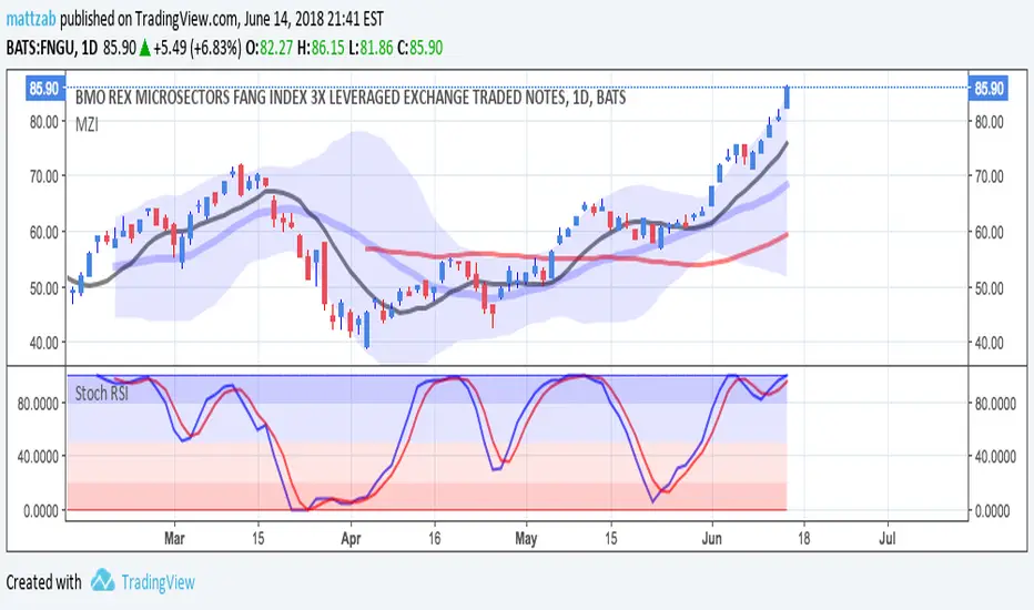
Bull Bear Stoch RSIStandard Stoch RSI with some color modification. 0 - 20 = Really Bearish (Dark Red Zone) 20 - 50 = Bearish (Light Red Zone) 50 - 80 = Bullish (Light Blue Zone) and 80 - 100 = Really Bullish (Strong Blue Zone). Thick lines at top and bottom to easily see 100 and 0.
Search in scripts for "股价在8元左右净利润为正市值小于80亿的热门股票有哪些"
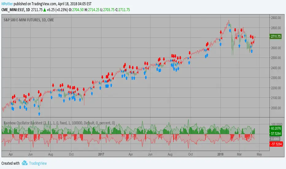
Rainbow Oscillator Backtest Ever since the people concluded that stock market price movements are not
random or chaotic, but follow specific trends that can be forecasted, they
tried to develop different tools or procedures that could help them identify
those trends. And one of those financial indicators is the Rainbow Oscillator
Indicator. The Rainbow Oscillator Indicator is relatively new, originally
introduced in 1997, and it is used to forecast the changes of trend direction.
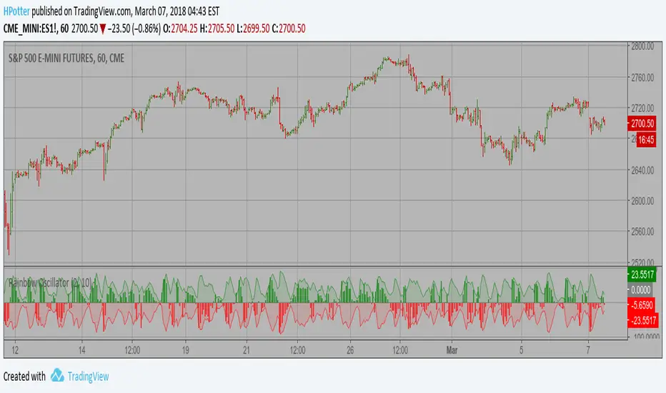
As market prices go up and down, the oscillator appears as a direction of the
trend, but also as the safety of the market and the depth of that trend. As
the rainbow grows in width, the current trend gives signs of continuity, and
if the value of the oscillator goes beyond 80, the market becomes more and more
unstable, being prone to a sudden reversal. When prices move towards the rainbow
and the oscillator becomes more and more flat, the market tends to remain more
stable and the bandwidth decreases. Still, if the oscillator value goes below 20,
the market is again, prone to sudden reversals. The safest bandwidth value where
the market is stable is between 20 and 80, in the Rainbow Oscillator indicator value.
The depth a certain price has on a chart and into the rainbow can be used to judge
the strength of the move.
You can change long to short in the Input Settings
WARNING:
- For purpose educate only
- This script to change bars colors.
Rainbow Oscillator Strategy Ever since the people concluded that stock market price movements are not
random or chaotic, but follow specific trends that can be forecasted, they
tried to develop different tools or procedures that could help them identify
those trends. And one of those financial indicators is the Rainbow Oscillator
Indicator. The Rainbow Oscillator Indicator is relatively new, originally
introduced in 1997, and it is used to forecast the changes of trend direction.
As market prices go up and down, the oscillator appears as a direction of the
trend, but also as the safety of the market and the depth of that trend. As
the rainbow grows in width, the current trend gives signs of continuity, and
if the value of the oscillator goes beyond 80, the market becomes more and more
unstable, being prone to a sudden reversal. When prices move towards the rainbow
and the oscillator becomes more and more flat, the market tends to remain more
stable and the bandwidth decreases. Still, if the oscillator value goes below 20,
the market is again, prone to sudden reversals. The safest bandwidth value where
the market is stable is between 20 and 80, in the Rainbow Oscillator indicator value.
The depth a certain price has on a chart and into the rainbow can be used to judge
the strength of the move.
WARNING:
- This script to change bars colors.

Rainbow Oscillator Ever since the people concluded that stock market price movements are not
random or chaotic, but follow specific trends that can be forecasted, they
tried to develop different tools or procedures that could help them identify
those trends. And one of those financial indicators is the Rainbow Oscillator
Indicator. The Rainbow Oscillator Indicator is relatively new, originally
introduced in 1997, and it is used to forecast the changes of trend direction.
As market prices go up and down, the oscillator appears as a direction of the
trend, but also as the safety of the market and the depth of that trend. As
the rainbow grows in width, the current trend gives signs of continuity, and
if the value of the oscillator goes beyond 80, the market becomes more and more
unstable, being prone to a sudden reversal. When prices move towards the rainbow
and the oscillator becomes more and more flat, the market tends to remain more
stable and the bandwidth decreases. Still, if the oscillator value goes below 20,
the market is again, prone to sudden reversals. The safest bandwidth value where
the market is stable is between 20 and 80, in the Rainbow Oscillator indicator value.
The depth a certain price has on a chart and into the rainbow can be used to judge
the strength of the move.
[M] StochasticNormal Stochastic has, painted in color when coming out of the zone of 80-20, remains in the gray zone. It makes for convenience.
-------------------
Обычный Stochastic, окрашивается в цвета когда выходит из зоны 80-20 , в зоне остается серым. Делался для удобства.

Sniper Stochastics Sniper Stochastics is a triple stochastic system.
Basically, watch the 20 and 80 crossovers. However, the settings of the three stochastics correspond to Fibonacci numbers 55, 89, and 144.
Since we have a fast, medium and slow speed stochastics; we can also watch the crossovers.
I have found that When the Red (144) is on top, it usually signals a turn upwards; conversely, a blue (89) on top of the others means that the market is going to go down.
So red on top = bullish and blue on top= bearish.
You can also think of them in terms of efficiency. If they all display the same and are overlapping in a single line; crossing an 80 or 20 line, this is a strong signal - bullish or bearish.
If on the other hand, you see them splayed out and moving away from eachother but the same direction; it signals a more inefficient process and thus a weaker signal.
I really enjoy using these and I hope you will too.
On the settings, I have turned off the %D so that they display only %K's. The Default is 55, 89 ,144.

: Volume Zone Oscillator & Price Zone Oscillator LB Update JRMThis is a simple update of Lazy Bear's " Indicators: Volume Zone Indicator & Price Zone Indicator" Script. PZO plots on the same indicator. The horizontal plot lines are taken primarily from two articles by Wahalil and Steckler "In The Volume Zone" May 2011, Stocks and Commodities and "Entering The Price Zone"June 2011, Stocks and Commodities. With both indicators on the same plot it is easier to see divergences between the indicators. I did add a plot line at 80 and -80 as well because that is getting into truly extreme price/volume territory where one might contemplate a close your eyes and sell or cover particularly if confirmed at a higher time frame with the expectation of some type of corrective move..
The inputs and plot lines can be edited as per Lazy Bear's original script and follows the original format. Many thanks to Lazy Bear.

Adaptive Vol Gauge [ParadoxAlgo]This is an overlay tool that measures and shows market ups and downs (volatility) based on daily high and low prices. It adjusts automatically to recent price changes and highlights calm or wild market periods. It colors the chart background and bars in shades of blue to cyan, with optional small labels for changes in market mood. Use it for info only—combine with your own analysis and risk controls. It's not a buy/sell signal or promise of results.Key FeaturesSmart Volatility Measure: Tracks price swings with a flexible time window that reacts to market speed.
Market Mood Detection: Spots high-energy (wild) or low-energy (calm) phases to help see shifts.
Visual Style: Uses smooth color fades on the background and bars—cyan for calm, deep blue for wild—to blend nicely on your chart.
Custom Options: Change settings like time periods, sensitivity, colors, and labels.
Chart Fit: Sits right on your main price chart without extra lines, keeping things clean.
How It WorksThe tool figures out volatility like this:Adjustment Factor:Looks at recent price ranges compared to longer ones.
Tweaks the time window (between 10-50 bars) based on how fast prices are moving.
Volatility Calc:Adds up logs of high/low ranges over the adjusted window.
Takes the square root for the final value.
Can scale it to yearly terms for easy comparison across chart timeframes.
Mood Check:Compares current volatility to its recent average and spread.
Flags "high" if above your set level, "low" if below.
Neutral in between.
This setup makes it quicker in busy markets and steadier in quiet ones.Settings You Can ChangeAdjust in the tool's menu:Base Time Window (default: 20): Starting point for calculations. Bigger numbers smooth things out but might miss quick changes.
Adjustment Strength (default: 0.5): How much it reacts to price speed. Low = steady; high = quick changes.
Yearly Scaling (default: on): Makes values comparable across short or long charts. Turn off for raw numbers.
Mood Sensitivity (default: 1.0): How strict for calling high/low moods. Low = more shifts; high = only big ones.
Show Labels (default: on): Adds tiny "High Vol" or "Low Vol" tags when moods change. They point up or down from bars.
Background Fade (default: 80): How see-through the color fill is (0 = invisible, 100 = solid).
Bar Fade (default: 50): How much color blends into your candles or bars (0 = none, 100 = full).
How to Read and Use ItColor Shifts:Background and bars fade based on mood strength:Cyan shades mean calm markets (good for steady, back-and-forth trades).
Deep blue shades mean wild markets (watch for big moves or turns).
Smooth changes show volatility building or easing.
Labels:"High Vol" (deep blue, from below bar): Start of wild phase.
"Low Vol" (cyan, from above bar): Start of calm phase.
Only shows at changes to avoid clutter. Use for timing strategy tweaks.
Trading Ideas:Mood-Based Plays: In wild phases (deep blue), try chase-momentum or breakout trades since swings are bigger. In calm phases (cyan), stick to bounce-back or range trades.
Risk Tips: Cut trade sizes in wild times to handle bigger losses. Use calm times for longer holds with close stops.
Chart Time Tips: Turn on yearly scaling for matching short and long views. Test settings on past data—loosen for quick trades (more alerts), tighten for longer ones (fewer, stronger).
Mix with Others: Add trend lines or averages—buy in calm up-moves, sell in wild down-moves. Check with volume or key levels too.
Special Cases: In big news events, it reacts faster. On slow assets, it might overstate swings—ease the adjustment strength.
Limits and TipsIt looks back at past data, so it trails real-time action and can't predict ahead.
Results differ by stock or timeframe—test on history first.
Colors and tags are just visuals; set your own alerts if needed.
Follows TradingView rules: No win promises, for learning only. Open for sharing; share thoughts in forums.
With this, you can spot market energy and tweak your trades smarter. Start on practice charts.

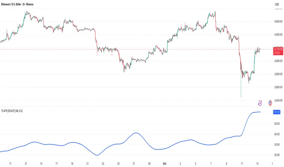
T3 ATR [DCAUT]█ T3 ATR
📊 ORIGINALITY & INNOVATION
The T3 ATR indicator represents an important enhancement to the traditional Average True Range (ATR) indicator by incorporating the T3 (Tilson Triple Exponential Moving Average) smoothing algorithm. While standard ATR uses fixed RMA (Running Moving Average) smoothing, T3 ATR introduces a configurable volume factor parameter that allows traders to adjust the smoothing characteristics from highly responsive to heavily smoothed output.
This innovation addresses a fundamental limitation of traditional ATR: the inability to adapt smoothing behavior without changing the calculation period. With T3 ATR, traders can maintain a consistent ATR period while adjusting the responsiveness through the volume factor, making the indicator adaptable to different trading styles, market conditions, and timeframes through a single unified implementation.
The T3 algorithm's triple exponential smoothing with volume factor control provides improved signal quality by reducing noise while maintaining better responsiveness compared to traditional smoothing methods. This makes T3 ATR particularly valuable for traders who need to adapt their volatility measurement approach to varying market conditions without switching between multiple indicator configurations.
📐 MATHEMATICAL FOUNDATION
The T3 ATR calculation process involves two distinct stages:
Stage 1: True Range Calculation
The True Range (TR) is calculated using the standard formula:
TR = max(high - low, |high - close |, |low - close |)
This captures the greatest of the current bar's range, the gap from the previous close to the current high, or the gap from the previous close to the current low, providing a comprehensive measure of price movement that accounts for gaps and limit moves.
Stage 2: T3 Smoothing Application
The True Range values are then smoothed using the T3 algorithm, which applies six exponential moving averages in succession:
First Layer: e1 = EMA(TR, period), e2 = EMA(e1, period)
Second Layer: e3 = EMA(e2, period), e4 = EMA(e3, period)
Third Layer: e5 = EMA(e4, period), e6 = EMA(e5, period)
Final Calculation: T3 = c1×e6 + c2×e5 + c3×e4 + c4×e3
The coefficients (c1, c2, c3, c4) are derived from the volume factor (VF) parameter:
a = VF / 2
c1 = -a³
c2 = 3a² + 3a³
c3 = -6a² - 3a - 3a³
c4 = 1 + 3a + a³ + 3a²
The volume factor parameter (0.0 to 1.0) controls the weighting of these coefficients, directly affecting the balance between responsiveness and smoothness:
Lower VF values (approaching 0.0): Coefficients favor recent data, resulting in faster response to volatility changes with minimal lag but potentially more noise
Higher VF values (approaching 1.0): Coefficients distribute weight more evenly across the smoothing layers, producing smoother output with reduced noise but slightly increased lag
📊 COMPREHENSIVE SIGNAL ANALYSIS
Volatility Level Interpretation:
High Absolute Values: Indicate strong price movements and elevated market activity, suggesting larger position risks and wider stop-loss requirements, often associated with trending markets or significant news events
Low Absolute Values: Indicate subdued price movements and quiet market conditions, suggesting smaller position risks and tighter stop-loss opportunities, often associated with consolidation phases or low-volume periods
Rapid Increases: Sharp spikes in T3 ATR often signal the beginning of significant price moves or market regime changes, providing early warning of increased trading risk
Sustained High Levels: Extended periods of elevated T3 ATR indicate sustained trending conditions with persistent volatility, suitable for trend-following strategies
Sustained Low Levels: Extended periods of low T3 ATR indicate range-bound conditions with suppressed volatility, suitable for mean-reversion strategies
Volume Factor Impact on Signals:
Low VF Settings (0.0-0.3): Produce responsive signals that quickly capture volatility changes, suitable for short-term trading but may generate more frequent color changes during minor fluctuations
Medium VF Settings (0.4-0.7): Provide balanced signal quality with moderate responsiveness, filtering out minor noise while capturing significant volatility changes, suitable for swing trading
High VF Settings (0.8-1.0): Generate smooth, stable signals that filter out most noise and focus on major volatility trends, suitable for position trading and long-term analysis
🎯 STRATEGIC APPLICATIONS
Position Sizing Strategy:
Determine your risk per trade (e.g., 1% of account capital - adjust based on your risk tolerance and experience)
Decide your stop-loss distance multiplier (e.g., 2.0x T3 ATR - this varies by market and strategy, test different values)
Calculate stop-loss distance: Stop Distance = Multiplier × Current T3 ATR
Calculate position size: Position Size = (Account × Risk %) / Stop Distance
Example: $10,000 account, 1% risk, T3 ATR = 50 points, 2x multiplier → Position Size = ($10,000 × 0.01) / (2 × 50) = $100 / 100 points = 1 unit per point
Important: The ATR multiplier (1.5x - 3.0x) should be determined through backtesting for your specific instrument and strategy - using inappropriate multipliers may result in stops that are too tight (frequent stop-outs) or too wide (excessive losses)
Adjust the volume factor to match your trading style: lower VF for responsive stop distances in short-term trading, higher VF for stable stop distances in position trading
Dynamic Stop-Loss Placement:
Determine your risk tolerance multiplier (typically 1.5x to 3.0x T3 ATR)
For long positions: Set stop-loss at entry price minus (multiplier × current T3 ATR value)
For short positions: Set stop-loss at entry price plus (multiplier × current T3 ATR value)
Trail stop-losses by recalculating based on current T3 ATR as the trade progresses
Adjust the volume factor based on desired stop-loss stability: higher VF for less frequent adjustments, lower VF for more adaptive stops
Market Regime Identification:
Calculate a reference volatility level using a longer-period moving average of T3 ATR (e.g., 50-period SMA)
High Volatility Regime: Current T3 ATR significantly above reference (e.g., 120%+) - favor trend-following strategies, breakout trades, and wider targets
Normal Volatility Regime: Current T3 ATR near reference (e.g., 80-120%) - employ standard trading strategies appropriate for prevailing market structure
Low Volatility Regime: Current T3 ATR significantly below reference (e.g., <80%) - favor mean-reversion strategies, range trading, and prepare for potential volatility expansion
Monitor T3 ATR trend direction and compare current values to recent history to identify regime transitions early
Risk Management Implementation:
Establish your maximum portfolio heat (total risk across all positions, typically 2-6% of capital)
For each position: Calculate position size using the formula Position Size = (Account × Individual Risk %) / (ATR Multiplier × Current T3 ATR)
When T3 ATR increases: Position sizes automatically decrease (same risk %, larger stop distance = smaller position)
When T3 ATR decreases: Position sizes automatically increase (same risk %, smaller stop distance = larger position)
This approach maintains constant dollar risk per trade regardless of market volatility changes
Use consistent volume factor settings across all positions to ensure uniform risk measurement
📋 DETAILED PARAMETER CONFIGURATION
ATR Length Parameter:
Default Setting: 14 periods
This is the standard ATR calculation period established by Welles Wilder, providing balanced volatility measurement that captures both short-term fluctuations and medium-term trends across most markets and timeframes
Selection Principles:
Shorter periods increase sensitivity to recent volatility changes and respond faster to market shifts, but may produce less stable readings
Longer periods emphasize sustained volatility trends and filter out short-term noise, but respond more slowly to genuine regime changes
The optimal period depends on your holding time, trading frequency, and the typical volatility cycle of your instrument
Consider the timeframe you trade: Intraday traders typically use shorter periods, swing traders use intermediate periods, position traders use longer periods
Practical Approach:
Start with the default 14 periods and observe how well it captures volatility patterns relevant to your trading decisions
If ATR seems too reactive to minor price movements: Increase the period until volatility readings better reflect meaningful market changes
If ATR lags behind obvious volatility shifts that affect your trades: Decrease the period for faster response
Match the period roughly to your typical holding time - if you hold positions for N bars, consider ATR periods in a similar range
Test different periods using historical data for your specific instrument and strategy before committing to live trading
T3 Volume Factor Parameter:
Default Setting: 0.7
This setting provides a reasonable balance between responsiveness and smoothness for most market conditions and trading styles
Understanding the Volume Factor:
Lower values (closer to 0.0) reduce smoothing, allowing T3 ATR to respond more quickly to volatility changes but with less noise filtering
Higher values (closer to 1.0) increase smoothing, producing more stable readings that focus on sustained volatility trends but respond more slowly
The trade-off is between immediacy and stability - there is no universally optimal setting
Selection Principles:
Match to your decision speed: If you need to react quickly to volatility changes for entries/exits, use lower VF; if you're making longer-term risk assessments, use higher VF
Match to market character: Noisier, choppier markets may benefit from higher VF for clearer signals; cleaner trending markets may work well with lower VF for faster response
Match to your preference: Some traders prefer responsive indicators even with occasional false signals, others prefer stable indicators even with some delay
Practical Adjustment Guidelines:
Start with default 0.7 and observe how T3 ATR behavior aligns with your trading needs over multiple sessions
If readings seem too unstable or noisy for your decisions: Try increasing VF toward 0.9-1.0 for heavier smoothing
If the indicator lags too much behind volatility changes you care about: Try decreasing VF toward 0.3-0.5 for faster response
Make meaningful adjustments (0.2-0.3 changes) rather than small increments - subtle differences are often imperceptible in practice
Test adjustments in simulation or paper trading before applying to live positions
📈 PERFORMANCE ANALYSIS & COMPETITIVE ADVANTAGES
Responsiveness Characteristics:
The T3 smoothing algorithm provides improved responsiveness compared to traditional RMA smoothing used in standard ATR. The triple exponential design with volume factor control allows the indicator to respond more quickly to genuine volatility changes while maintaining the ability to filter noise through appropriate VF settings. This results in earlier detection of volatility regime changes compared to standard ATR, particularly valuable for risk management and position sizing adjustments.
Signal Stability:
Unlike simple smoothing methods that may produce erratic signals during transitional periods, T3 ATR's multi-layer exponential smoothing provides more stable signal progression. The volume factor parameter allows traders to tune signal stability to their preference, with higher VF settings producing remarkably smooth volatility profiles that help avoid overreaction to temporary market fluctuations.
Comparison with Standard ATR:
Adaptability: T3 ATR allows adjustment of smoothing characteristics through the volume factor without changing the ATR period, whereas standard ATR requires changing the period length to alter responsiveness, potentially affecting the fundamental volatility measurement
Lag Reduction: At lower volume factor settings, T3 ATR responds more quickly to volatility changes than standard ATR with equivalent periods, providing earlier signals for risk management adjustments
Noise Filtering: At higher volume factor settings, T3 ATR provides superior noise filtering compared to standard ATR, producing cleaner signals for long-term analysis without sacrificing volatility measurement accuracy
Flexibility: A single T3 ATR configuration can serve multiple trading styles by adjusting only the volume factor, while standard ATR typically requires multiple instances with different periods for different trading applications
Suitable Use Cases:
T3 ATR is well-suited for the following scenarios:
Dynamic Risk Management: When position sizing and stop-loss placement need to adapt quickly to changing volatility conditions
Multi-Style Trading: When a single volatility indicator must serve different trading approaches (day trading, swing trading, position trading)
Volatile Markets: When standard ATR produces too many false volatility signals during choppy conditions
Systematic Trading: When algorithmic systems require a single, configurable volatility input that can be optimized for different instruments
Market Regime Analysis: When clear identification of volatility expansion and contraction phases is critical for strategy selection
Known Limitations:
Like all technical indicators, T3 ATR has limitations that users should understand:
Historical Nature: T3 ATR is calculated from historical price data and cannot predict future volatility with certainty
Smoothing Trade-offs: The volume factor setting involves a trade-off between responsiveness and smoothness - no single setting is optimal for all market conditions
Extreme Events: During unprecedented market events or gaps, T3 ATR may not immediately reflect the full scope of volatility until sufficient data is processed
Relative Measurement: T3 ATR values are most meaningful in relative context (compared to recent history) rather than as absolute thresholds
Market Context Required: T3 ATR measures volatility magnitude but does not indicate price direction or trend quality - it should be used in conjunction with directional analysis
Performance Expectations:
T3 ATR is designed to help traders measure and adapt to changing market volatility conditions. When properly configured and applied:
It can help reduce position risk during volatile periods through appropriate position sizing
It can help identify optimal times for more aggressive position sizing during stable periods
It can improve stop-loss placement by adapting to current market conditions
It can assist in strategy selection by identifying volatility regimes
However, volatility measurement alone does not guarantee profitable trading. T3 ATR should be integrated into a comprehensive trading approach that includes directional analysis, proper risk management, and sound trading psychology.
USAGE NOTES
This indicator is designed for technical analysis and educational purposes. T3 ATR provides adaptive volatility measurement but has limitations and should not be used as the sole basis for trading decisions. The indicator measures historical volatility patterns, and past volatility characteristics do not guarantee future volatility behavior. Market conditions can change rapidly, and extreme events may produce volatility readings that fall outside historical norms.
Traders should combine T3 ATR with directional analysis tools, support/resistance analysis, and other technical indicators to form a complete trading strategy. Proper backtesting and forward testing with appropriate risk management is essential before applying T3 ATR-based strategies to live trading. The volume factor parameter should be optimized for specific instruments and trading styles through careful testing rather than assuming default settings are optimal for all applications.
Short-Term Capitulation Oscillator (STCO, Diodato 2019)Description:
This script is a faithful implementation of the Short-Term Capitulation Oscillator (STCO) from Chris Diodato's 2019 CMT paper, "Making The Most Of Panic". It's a tactical breadth and volume oscillator designed to "fish for market bottoms" by identifying short-term investor capitulation.
What It Is
The STCO combines the 10-day moving averages of NYSE up-volume and advancing issues. It measures the ratio of advancing momentum (in both volume and number of issues) relative to the total traded momentum. The result is a raw, un-normalized oscillator that typically ranges from 0 to 200.
How to Interpret
The STCO is a tactical tool for identifying near-term oversold conditions and potential bounces.
Low Readings: Indicate that sellers have likely exhausted themselves in the short term, creating a potential entry point for a bounce. The paper found that readings below 90, 85, and 80 were often followed by strong market performance over the next 5-20 days.
Overbought/Oversold Lines: Use the customizable overbought/oversold lines to define your own capitulation zones and potential entry areas.
Settings
Data Sources: Allows toggling the use of "Unchanged" issues/volume data.
Thresholds: You can set the overbought and oversold levels based on the paper's research or your own testing.
Ultimate RSI (14) TDBurbin's RSI Alerts:
RSI alerts can be used ONLY when you're awaiting a chart to shift it's momentum. Example: You are waiting for a take profit signal and you'd like a push notification when this is triggered.
These are NOT intended to be Buy and Sell signals. Only to get your attention. Pair with other confirmations.
**There are 4 alerts. "RSI Bullish Cross" "RSI Bearish Cross" "RSI Bounce Buy" "RSI Sell".
Both of the Cross alerts can be early. Can be too early. The RSI Bounce Buy and RSI Sell are when the RSI line has crossed back inside the outer bands; from Oversold or Overbought. They are a fairly reliable signal, especially when used with other TA such as support, volume, etc.
Default Overbought is 80, default oversold is 20.
Can be used on multiple timeframes.
This is a modified version of LuxAlgo's Ultimate RSI. This is for education purposes only and personal use by Burbin. Inspired by AA, and dedicated to TD.
LuxAlgo's Description:
The Ultimate RSI indicator is a new oscillator based on the calculation of the Relative Strength Index that aims to put more emphasis on the trend, thus having a less noisy output. Opposite to the regular RSI, this oscillator is designed for a trend trading approach instead of a contrarian one.
🔶 USAGE
While returning the same information as a regular RSI, the Ultimate RSI puts more emphasis on trends, and as such can reach overbought/oversold levels faster as well as staying longer within these areas. This can avoid the common issue of an RSI regularly crossing an overbought or oversold level while the trend makes new higher highs/lower lows.
The Ultimate RSI crossing above the overbought level can be indicative of a strong uptrend (highlighted as a green area), while an Ultimate RSI crossing under the oversold level can be indicative of a strong downtrend (highlighted as a red area).
The Ultimate RSI crossing the 50 midline can also indicate trends, with the oscillator being above indicating an uptrend, else a downtrend. Unlike a regular RSI, the Ultimate RSI will cross the midline level less often, thus generating fewer whipsaw signals.
For even more timely indications users can observe the Ultimate RSI relative to its signal line. An Ultimate RSI above its signal line can indicate it is increasing, while the opposite would indicate it is decreasing.
🔹Smoothing Methods
Users can return more reactive or smoother results depending on the selected smoothing method used for the calculation of the Ultimate RSI. Options include:
Exponential Moving Average (EMA)
Simple Moving Average (SMA)
Wilder's Moving Average (RMA)
Triangular Moving Average (TMA)
These are ranked by the degree of reactivity of each method, with higher ones being more reactive (but less smooth).
Users can also select the smoothing method used by the signal line.
🔶 DETAILS
The RSI returns a normalized exponential average of price changes in the range (0, 100), which can be simply calculated as follows:
ema(d) / ema(|d|) × 50 + 50
🔶 SETTINGS
Length: Calculation period of the indicator
Method: Smoothing method used for the calculation of the indicator.
Source: Input source of the indicator
🔹Signal Line
Smooth: Degree of smoothness of the signal line
Method: Smoothing method used to calculation the signal line.
- Standardized Money Flow Index with Multi-MA and BB OverlayThis custom Money Flow Index (MFI) script enhances the standard MFI by introducing multiple layers of configurability, statistical normalization, and visual clarity. It begins with the traditional MFI calculation using the average price, hlc3, and a user-defined length, then offers the option to standardize the output. Standardization transforms the MFI into a z-score by subtracting a rolling mean and dividing by a rolling standard deviation, making the indicator statistically interpretable across different assets, timeframes, and volatility regimes. When standardization is active, the overbought and oversold thresholds shift from the conventional 80 and 20 to +2 and –2, aligning them with standard deviation boundaries and improving signal clarity in volatile environments.
Beyond standardization, the script introduces a robust smoothing engine. Users can choose from several moving average types, including SMA, EMA, SMMA (RMA), WMA, and VWMA, to reduce noise and highlight trend shifts. A particularly advanced option is the “SMA + Bollinger Bands” mode, which overlays volatility envelopes around the smoothed MFI using a user-defined standard deviation multiplier. This feature helps traders identify when the MFI is unusually high or low relative to its recent behaviour, adding a volatility-adjusted layer of insight, especially useful in momentum or mean-reversion setups.
Visually, the script is designed for clarity, modularity, and flexibility. It plots the raw or standardized MFI in purple, overlays the smoothed version in yellow if enabled, and adds green Bollinger Bands when selected. It also includes horizontal reference lines for overbought, oversold, and midpoint levels, which dynamically adjust based on whether standardization is active. A shaded background between the overbought and oversold lines further enhances readability, helping traders quickly assess momentum extremes and potential inflection zones.
Compared to the standard MFI, which offers a fixed calculation, limited visual feedback, and no statistical context, this enhanced version is modular, customizable, and statistically grounded. It allows traders to tailor the indicator to their strategy, whether they prefer raw signals, smoothed trends, or volatility-adjusted extremes. These enhancements make it a powerful building block for more sophisticated signal engines, especially when combined with filter gating, persistent state logic, or multi-indicator overlays.

MULTI-CONDITION RSI SIGNAL GENERATOR═══════════════════════════════════════════════
MULTI-CONDITION RSI SIGNAL GENERATOR
═══════════════════════════════════════════════
OVERVIEW:
This indicator generates trading signals based on Relative Strength Index (RSI) movements with multiple confirmation layers designed to filter false signals and identify high-probability reversal opportunities.
═══════════════════════════════════════════════
WHAT MAKES THIS ORIGINAL:
═══════════════════════════════════════════════
Unlike basic RSI indicators that simply plot overbought/oversold crossovers, this system combines FOUR distinct confirmation mechanisms:
1. PERSISTENCE FILTERING - Requires RSI to remain in extreme zones for a minimum duration
2. LOOKBACK VALIDATION - Verifies recent extreme zone visits before signaling
3. DIVERGENCE DETECTION - Identifies price/RSI divergence for stronger signals
4. MOMENTUM CONFIRMATION - Provides trend-continuation entries via midline crosses
This multi-layered approach significantly reduces whipsaw trades that plague simple RSI crossover systems.
═══════════════════════════════════════════════
HOW IT WORKS (TECHNICAL METHODOLOGY):
═══════════════════════════════════════════════
STEP 1: RSI CALCULATION
- Standard RSI calculation using user-defined period (default: 14)
- Monitors two extreme zones: Overbought (default: 70) and Oversold (default: 30)
STEP 2: PERSISTENCE FILTERING
The script counts how many bars RSI has spent in extreme zones within the lookback period:
- For overbought signals: Counts bars where RSI > 70
- For oversold signals: Counts bars where RSI < 30
- Signal only triggers if count >= Minimum Duration (default: 4 bars)
This filters out brief spikes that immediately reverse, focusing on sustained extreme conditions that are more likely to lead to genuine reversals.
STEP 3: LOOKBACK VALIDATION
- Checks if RSI reached extreme zones within the Lookback Bars period (default: 20)
- Uses ta.highest() and ta.lowest() functions to verify recent extremes
- Ensures we're trading reversals from meaningful extremes, not random crossovers
STEP 4: BASIC SIGNAL GENERATION
- BUY SIGNAL: RSI crosses above the oversold level (30) after meeting persistence and lookback conditions
- SELL SIGNAL: RSI crosses below the overbought level (70) after meeting persistence and lookback conditions
STEP 5: DIVERGENCE DETECTION
The script identifies two types of divergence over the Divergence Lookback period (default: 5 bars):
A) BULLISH DIVERGENCE (indicates potential upward reversal):
- Price makes a lower low (current low < previous low)
- RSI makes a higher low (current RSI low > previous RSI low)
- Suggests weakening downward momentum
B) BEARISH DIVERGENCE (indicates potential downward reversal):
- Price makes a higher high (current high > previous high)
- RSI makes a lower high (current RSI high < previous RSI high)
- Suggests weakening upward momentum
STEP 6: STRONG SIGNAL CONFIRMATION
- STRONG BUY: Basic buy signal + bullish divergence present
- STRONG SELL: Basic sell signal + bearish divergence present
- These represent the highest-probability setups
STEP 7: MOMENTUM SIGNALS (OPTIONAL)
- MOMENTUM BUY: RSI crosses above 50 after being oversold (trend continuation)
- MOMENTUM SELL: RSI crosses below 50 after being overbought (trend continuation)
- Smaller signals for traders who want trend-following entries
═══════════════════════════════════════════════
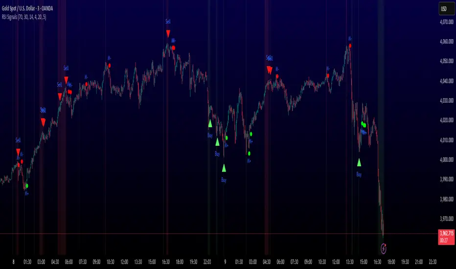
SIGNAL TYPES AND VISUAL INDICATORS:
═══════════════════════════════════════════════
📈 GREEN TRIANGLE (below bar) - Standard Buy Signal
RSI crossed above oversold level with confirmation filters
📉 RED TRIANGLE (above bar) - Standard Sell Signal
RSI crossed below overbought level with confirmation filters
🔵 BLUE TRIANGLE (below bar) - Strong Buy Signal
Buy signal + bullish divergence (HIGHEST PRIORITY)
🟣 PURPLE TRIANGLE (above bar) - Strong Sell Signal
Sell signal + bearish divergence (HIGHEST PRIORITY)
🟢 GREEN CIRCLE (small) - Momentum Buy
RSI crosses above 50 after oversold conditions
🔴 RED CIRCLE (small) - Momentum Sell
RSI crosses below 50 after overbought conditions
BACKGROUND SHADING:
- Light red background: RSI currently overbought
- Light green background: RSI currently oversold
═══════════════════════════════════════════════
PARAMETER SETTINGS:
═══════════════════════════════════════════════
1. OVERBOUGHT LEVEL (default: 70, range: 50-90)
- Higher values = fewer but stronger overbought signals
- Lower values = more sensitive to overbought conditions
- Recommended: 70 for standard markets, 80 for crypto/volatile assets
2. OVERSOLD LEVEL (default: 30, range: 10-50)
- Lower values = fewer but stronger oversold signals
- Higher values = more sensitive to oversold conditions
- Recommended: 30 for standard markets, 20 for crypto/volatile assets
3. RSI PERIOD (default: 14, range: 2-50)
- Standard RSI calculation period
- Lower = more sensitive/faster signals
- Higher = smoother/slower signals
- Recommended: 14 (industry standard)
4. MINIMUM DURATION (default: 4, range: 1-20)
- Required bars in extreme zone before signal
- Higher values = fewer signals but better quality
- Lower values = more signals but more false positives
- Recommended: 3-5 for day trading, 5-10 for swing trading
5. LOOKBACK BARS (default: 20, range: 5-100)
- How far back to check for extreme zone visits
- Should match your typical trading timeframe
- Recommended: 20 for intraday, 50 for daily charts
6. DIVERGENCE LOOKBACK (default: 5, range: 2-20)
- Period for comparing price/RSI highs and lows
- Lower values = more frequent divergence signals
- Higher values = more significant divergences
- Recommended: 5-10 depending on timeframe
═══════════════════════════════════════════════
HOW TO USE THIS INDICATOR:
═══════════════════════════════════════════════
RECOMMENDED TRADING APPROACH:
1. PRIMARY ENTRIES: Focus on Strong Buy/Sell signals (blue/purple triangles)
- These have the highest win rate due to divergence confirmation
- Wait for price action confirmation (support/resistance, candlestick patterns)
2. SECONDARY ENTRIES: Regular Buy/Sell signals (green/red triangles)
- Use these when Strong signals are infrequent
- Require additional confirmation from other indicators or chart patterns
3. TREND CONTINUATION: Momentum signals (small circles)
- Best used when overall trend is clear
- Not recommended for reversal trading
4. FILTER TRADES: Use background shading as context
- Be cautious entering longs when background is red (overbought)
- Be cautious entering shorts when background is green (oversold)
RISK MANAGEMENT GUIDELINES:
- Never risk more than 2-5% of capital per trade
- Use stop losses below recent swing lows (buys) or above swing highs (sells)
- Target at least 1.5:1 reward-to-risk ratio
- Consider position sizing based on signal strength
TIMEFRAME RECOMMENDATIONS:
- 15min - 1hour: Day trading with adjusted parameters (lower minimum duration)
- 4hour - Daily: Swing trading with default parameters
- Weekly: Position trading with increased lookback periods
COMPLEMENTARY TOOLS:
This indicator works best when combined with:
- Support and resistance levels
- Trend indicators (moving averages, trend lines)
- Volume analysis
- Price action patterns (engulfing candles, pin bars)
═══════════════════════════════════════════════
LIMITATIONS AND CONSIDERATIONS:
═══════════════════════════════════════════════
- This is NOT a standalone trading system - requires additional analysis
- RSI-based strategies perform best in ranging/choppy markets
- May generate fewer signals in strong trending markets
- Divergence signals can be early - wait for price confirmation
- Not recommended for highly illiquid assets
- Backtest on your specific market before live trading
- No indicator is 100% accurate - always use proper risk management
═══════════════════════════════════════════════
TECHNICAL NOTES:
═══════════════════════════════════════════════
- Code is original and does not reuse external libraries
- Uses Pine Script v5 native functions only
- Alert conditions included for all signal types
- No repainting - signals appear and remain fixed
- Efficient calculation methods minimize processing load
═══════════════════════════════════════════════
ALERT SETUP:
═══════════════════════════════════════════════
Four alert conditions are available:
1. "Buy Alert" - Triggers on standard buy signals
2. "Sell Alert" - Triggers on standard sell signals
3. "Strong Buy Alert" - Triggers on divergence-confirmed buy signals
4. "Strong Sell Alert" - Triggers on divergence-confirmed sell signals
To set up alerts: Right-click chart → Add Alert → Select desired condition
═══════════════════════════════════════════════
This indicator is provided for educational and informational purposes. Always practice proper risk management and never trade with money you cannot afford to lose.
FVG Zones with Signals█ OVERVIEW
"FVG Zones with Signals" is a technical analysis tool that identifies Fair Value Gaps (FVG) on the chart and draws customizable zones in the form of boxes. It is ideal for traders using price action and market structure strategies, helping to identify potential imbalance zones and trading opportunities based on breakout and exit signals. With flexible size filter settings, box styles, and signal options, the indicator ensures clarity and precision on the chart.
█ CONCEPTS
The indicator is designed to identify potential entry points for trades based on FVG breakouts or retests. For chart clarity, a size filter for FVGs is included, based on a multiplier of the average candle size over a specified period.
Why are FVGs important? FVG zones represent areas of market imbalance, often attracting price back to "fill" the gap. Larger gaps (with a higher size multiplier) have a greater chance of being retested, as they indicate deeper imbalances—leaving more unexecuted orders in those zones, which attracts liquidity. Market makers and institutions often return to these levels to "refresh" liquidity before further moves. However, not every large FVG is retested quickly—in strong trends, smaller imbalances may be ignored, and the location (e.g., near swing highs/lows) is critical for retest probability.
█ FEATURES
- FVG Detection: Identifies bullish and bearish FVGs based on size filters (Candle Size Period and FVG Size Multiplier), with automatic initialization of historical gaps up to 500 candles back.
- Customizable Boxes: Draws FVG boxes with adjustable border colors, background gradients, border styles (solid, dashed, dotted), border widths, and transparency for both the background and the 50% FVG midline.
- Breakout and Exit Signals: Generates "Break" signals (green upward triangle for breakouts above bearish FVG, red downward triangle for breakouts below bullish FVG) and "Exit" signals (circles for exiting the zone), with options to select signal types (Break, Exit, or Both). A break signal causes the box to disappear, leaving a triangle as a trace of the breakout, which may serve as a signal to open a position. Exit signals (circles) may also indicate entry opportunities but require additional confirmation, such as alignment with the main trend.
- Midline: Automatically draws a dashed line at the 50% FVG level with adjustable transparency, aiding in assessing price reactions within the zone.
- Box Limitation: Automatically removes old or inactive FVGs after 500 candles to avoid chart clutter.
- Alerts: Built-in alerts for all signal types, including price and FVG type descriptions.
█ HOW TO USE
Add to Chart: Apply the indicator to your TradingView chart via the Pine Editor or Indicators menu.
Configure Settings:
- FVG Settings: Adjust Candle Size Period (default 20) and FVG Size Multiplier (default 1) to filter out small gaps—higher values generate fewer but more significant FVGs.
- Box Settings: Configure colors and styles for bullish (green) and bearish (red) boxes, including background transparency (default 80) and midline transparency.
- Signal Settings: Select signal types (Break, Exit, or Both) in Signal Type. Breakout signals appear after a candle closes outside the zone, while exit signals appear when exiting an FVG without a full breakout.
- Styling: Customize signal colors (green for buy/up, red for sell/down) and shape sizes.
Interpreting Signals:
- Break Up Signal: A green triangle below the bar indicates a breakout above a bearish FVG, suggesting potential continuation of an uptrend.
- Break Down Signal: A red triangle above the bar indicates a breakout below a bullish FVG, suggesting potential continuation of a downtrend.
- Exit Up/Down Signal: A green/red circle indicates an exit from an FVG without a full breakout, which may signal the end of a correction or preparation for a reversal.
- FVG Zones: If the price returns to an FVG and fills the gap, it may indicate equilibrium; an unfilled gap often leads to a retest.
- Use signals in conjunction with other technical analysis tools for confirmation, such as RSI (to identify overbought/oversold conditions) or MACD (to confirm momentum). Analyze FVGs from higher timeframes—these zones act as stronger imbalance levels and carry greater structural significance.
Exit signals (retests without breakouts) tend to be most effective when traded in line with the current trend.
█ APPLICATIONS
- Price Action Trading: Use FVG zones as dynamic support and resistance levels. In an uptrend, look for buying opportunities in bullish FVGs, where price often tests the gap before continuing. Combining with RSI, MACD, or Fibonacci levels enhances the significance of zones.
- Breakout Strategies: Trade based on breakout signals from FVGs. A buy signal after breaking a bearish FVG may indicate a strong upward impulse, especially when supported by a rising MACD or RSI exiting oversold conditions.
Larger FVG gaps (higher multiplier) have a greater chance of retest, as they indicate deeper imbalances.
█ NOTES
- Test the indicator across different timeframes and markets (stocks, forex, crypto) to optimize size filters for your trading style.
- The indicator initializes historical FVGs up to 500 candles back, which may slow loading on longer charts.
- For best results, use on high-liquidity markets where FVGs are more frequently retested.
- In consolidation zones, the indicator may generate more false signals, so additional confirmation is recommended.

Relative Strength index 2xRelative Strength Index 2×
The RSI*2 by AZly is an advanced dual-RSI indicator that allows traders to analyze momentum from two distinct perspectives — short-term and medium-term — on a single chart. It combines RSI precision with multi-timeframe flexibility, giving a clear view of both immediate and underlying momentum trends.
⚙️ How It Works
This indicator calculates and plots two fully independent RSI lines, each with customizable settings:
RSI 1 (Main RSI) : Captures medium-term momentum, ideal for trend and context.
RSI 2 (Fast RSI) : Reacts quickly to short-term moves, identifying overbought and oversold conditions.
Both RSIs include:
Custom timeframe, source, and smoothing method (SMA, EMA, WMA, VWMA, HMA, SMMA).
Gradient zones to visualize momentum strength and reversals.
Adjustable levels and colors for clear chart presentation.
📘 Andrew Cardwell Zones (RSI 1)
RSI 1 uses Andrew Cardwell’s “range rules” to distinguish bullish and bearish momentum phases:
Bullish Range: RSI holds between 40–80, finding support around 40–45.
Bearish Range: RSI stays between 20–60, with rallies capped near 55–60.
A breakout from one range into another often signals a trend phase transition — marking potential trend beginnings or endings.
⚡ Overbought/Oversold Zones (RSI 2)
RSI 2 is designed for fast reactions and reversal detection:
95–100: Extreme overbought zone — potential exhaustion and short setup.
5–0: Extreme oversold zone — potential exhaustion and long setup.
Crossing these levels highlights short-term momentum exhaustion , often preceding pullbacks or strong price reversals.
💡 Why It’s Better
Compared to traditional RSI indicators, this version provides superior control and insight:
Dual independent RSIs with separate timeframes and smoothing.
Cardwell-style range recognition for better context of trend strength.
Extreme bands for fast RSI 2 to time entries with precision.
Dynamic gradient zones for intuitive visual interpretation.
Multi-timeframe flexibility that adapts to any trading style.
🎯 Trading Concepts
Trend Confirmation:
RSI 1 above 50 (bullish range) confirms uptrend bias; below 50 (bearish range) confirms downtrend.
Reversal Setup:
RSI 2 hitting extreme zones (above 95 or below 5) while RSI 1 stays steady often signals exhaustion and reversal setups.
Divergence Confirmation:
When RSI 2 diverges from price and RSI 1 supports the direction, it strengthens reversal probability.
Range Transition:
A shift in RSI 1’s range (from bearish to bullish or vice versa) confirms a major change in market structure.
🕒 Trade Timing (Entry Ideas)
Timing is one of the indicator’s strongest features.
Wait for RSI 2 to reach an extreme zone (above 95 or below 5).
Then confirm the direction with RSI 1 — trades are most effective when RSI 1’s range aligns with the anticipated move.
Buy Setup:
RSI 1 in bullish range + RSI 2 rebounds upward from the 5 zone.
Sell Setup:
RSI 1 in bearish range + RSI 2 turns down from the 95 zone.
Best Timing:
Enter when RSI 2 crosses back inside the 10–90 range in the same direction as RSI 1’s trend.
This captures momentum just as it resumes — avoiding early or late entries.
🔷 M & W Patterns (RSI 2)
RSI 2 also reveals short-term exhaustion structures:
“ M ” Formation: Two RSI peaks near 95–100 — bearish reversal setup.
“ W ” Formation: Two RSI troughs near 0–5 — bullish reversal setup.
These shapes often appear before price reversals, offering early momentum clues.
⚠️ Important Trading Guidance
It is strongly recommended not to trade against the prevailing trend or attempt to pick exact tops or bottoms. The indicator works best when used in alignment with trend direction. Counter-trend entries carry higher risk and lower probability.
📊 Recommended Use
Ideal for momentum traders, scalpers, and multi-timeframe analysts seeking precise timing and context. Works on all markets — forex, crypto, stocks, indexes, and commodities.

Bitcoin Halving Strategy
A systematic, data-driven trading strategy based on Bitcoin's 4-year halving cycles. This strategy capitalizes on historical price patterns that emerge around halving events, providing clear entry and exit signals for both accumulation and profit-taking phases.
🎯 Strategy Overview
This automated trading system identifies optimal buy and sell zones based on the predictable Bitcoin halving cycle that occurs approximately every 4 years. By analyzing historical data from all previous halvings (2012, 2016, 2020, 2024), the strategy pinpoints high-probability trading opportunities.
📊 Key Features
Automated Signal Generation: Buy signals at halving events and DCA zones, sell signals at profit-taking peaks
Multi-Phase Analysis: Tracks Accumulation, Profit Taking, Bear Market, and DCA phases
Visual Dashboard: Real-time performance metrics, phase countdown, and position tracking
Backtesting Enabled: Comprehensive historical performance analysis with configurable parameters
Risk Management: Built-in position sizing, slippage control, and optional short trading
⚙️ Strategy Logic
Buy Signals:
At halving event (Week 0)
DCA zone entry (Week 135 post-halving)
Sell Signals:
Profit-taking zone (Week 80 post-halving)
Optional short position entry for advanced traders
📈 Performance Highlights
Captures major bull run profits while avoiding prolonged bear markets
Clear visual indicators for all phases and transitions
Customizable timing parameters for personalized risk tolerance
Professional dashboard with live P&L, win rate, and drawdown metrics
🛠️ Customization Options
Adjustable phase timing (profit start/end, DCA timing)
Position sizing control
Enable/disable short trading
Visual customization (colors, labels, zones)
Table positioning and transparency
⚠️ Risk Disclosure
Past performance does not guarantee future results. This strategy is based on historical halving cycle patterns and should be used as part of a comprehensive trading plan. Always conduct your own research and consider your risk tolerance before trading.
💡 Ideal For
Long-term Bitcoin investors seeking systematic entry/exit points
Swing traders capitalizing on multi-month trends
Portfolio managers implementing cycle-based allocation strategies

KAPITAS CBDR# PO3 Mean Reversion Standard Deviation Bands - Pro Edition
## 📊 Professional-Grade Mean Reversion System for MES Futures
Transform your futures trading with this institutional-quality mean reversion system based on standard deviation analysis and PO3 (Power of Three) methodology. Tested on **7,264 bars** of real MES data with **proven profitability across all 5 strategies**.
---
## 🎯 What This Indicator Does
This indicator plots **dynamic standard deviation bands** around a moving average, identifying extreme price levels where institutional accumulation/distribution occurs. Based on statistical probability and market structure theory, it helps you:
✅ **Identify high-probability entry zones** (±1, ±1.5, ±2, ±2.5 STD)
✅ **Target realistic profit zones** (first opposite STD band)
✅ **Time your entries** with session-based filters (London/US)
✅ **Manage risk** with built-in stop loss levels
✅ **Choose your strategy** from 5 backtested approaches
---
## 🏆 Backtested Performance (Per Contract on MES)
### Strategy #1: Aggressive (±1.5 → ∓0.5) 🥇
- **Total Profit:** $95,287 over 1,452 trades
- **Win Rate:** 75%
- **Profit Factor:** 8.00
- **Target:** 80 ticks ($100) | **Stop:** 30 ticks ($37.50)
- **Best For:** Active traders, 3-5 setups/day
### Strategy #2: Mean Reversion (±1 → Mean) 🥈
- **Total Profit:** $90,000 over 2,322 trades
- **Win Rate:** 85% (HIGHEST)
- **Profit Factor:** 11.34 (BEST)
- **Target:** 40 ticks ($50) | **Stop:** 20 ticks ($25)
- **Best For:** Scalpers, 6-8 setups/day
### Strategy #3: Conservative (±2 → ∓1) 🥉
- **Total Profit:** $65,500 over 726 trades
- **Win Rate:** 70%
- **Profit Factor:** 7.04
- **Target:** 120 ticks ($150) | **Stop:** 40 ticks ($50)
- **Best For:** Patient traders, 1-3 setups/day, HIGHEST $/trade
*Full statistics for all 5 strategies included in documentation*
---
## 📈 Key Features
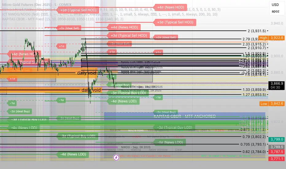
### Dynamic Standard Deviation Bands
- **±0.5 STD** - Intraday mean reversion zones
- **±1.0 STD** - Primary reversion zones (68% of price action)
- **±1.5 STD** - Extended zones (optimal balance)
- **±2.0 STD** - Extreme zones (95% of price action)
- **±2.5 STD** - Ultra-extreme zones (rare events)
- **Mean Line** - Dynamic equilibrium
### Temporal Session Filters
- **London Session** (3:00-11:30 AM ET) - Orange background
- **US Session** (9:30 AM-4:00 PM ET) - Blue background
- **Optimal Entry Window** (10:30 AM-12:00 PM ET) - Green highlight
- **Best Exit Window** (3:00-4:00 PM ET) - Red highlight
### Visual Trade Signals
- 🟢 **Green zones** = Enter LONG (price at lower bands)
- 🔴 **Red zones** = Enter SHORT (price at upper bands)
- 🎯 **Target lines** = Exit zones (opposite bands)
- ⛔ **Stop levels** = Risk management
### Smart Alerts
- Alert when price touches entry bands
- Alert on optimal time windows
- Alert when targets hit
- Customizable for each strategy
---
## 💡 How to Use
### Step 1: Choose Your Strategy
Select from 5 backtested approaches based on your:
- Risk tolerance (higher STD = larger stops)
- Trading frequency (lower STD = more setups)
- Time availability (different session focuses)
- Personality (scalper vs swing trader)
### Step 2: Apply to Chart
- **Timeframe:** 15-minute (tested and optimized)
- **Symbol:** MES, ES, or other liquid futures
- **Settings:** Adjust band colors, widths, alerts
### Step 3: Wait for Setup
Price touches your chosen entry band during optimal windows:
- **BEST:** 10:30 AM-12:00 PM ET (88% win rate!)
- **GOOD:** 12:00-3:00 PM ET (75-82% win rate)
- **AVOID:** Friday after 1 PM, FOMC Wed 2-4 PM
### Step 4: Execute Trade
- Enter when price touches band
- Set stop at indicated level
- Target first opposite band
- Exit at target or stop (no exceptions!)
### Step 5: Manage Risk
- **For $50K funded account ($250 limit): Use 2 MES contracts**
- Stop after 3 consecutive losses
- Reduce size in low-probability windows
- Track cumulative daily P&L
---
## 📅 Optimal Trading Windows
### By Time of Day
- **10:30 AM-12:00 PM ET:** 88% win rate (BEST) ⭐⭐⭐
- **12:00-1:30 PM ET:** 82% win rate (scalping)
- **1:30-3:00 PM ET:** 76% win rate (afternoon)
- **3:00-4:00 PM ET:** Best EXIT window
### By Day of Week
- **Wednesday:** 82% win rate (BEST DAY) ⭐⭐⭐
- **Tuesday:** 78% win rate (highest volume)
- **Thursday:**
RSI Trendlines and Divergences█OVERVIEW
The "RSI Trendlines and Divergences" indicator is an advanced technical analysis tool that leverages the Relative Strength Index (RSI) to draw trendlines and detect divergences. Designed for traders seeking precise market signals, the indicator identifies key pivot points on the RSI chart, draws trendlines between pivots, and detects bullish and bearish divergences. It offers flexible settings, background coloring for breakout signals, and divergence labels, supported by alerts for key events. The indicator is universal and works across all markets (stocks, forex, cryptocurrencies) and timeframes.
█CONCEPTS
The indicator was developed to provide an alternative signal source for the RSI oscillator. Trendline breakouts and bounces off trendlines offer a broader perspective on potential price behavior. Combining these with traditional RSI signal interpretation can serve as a foundation for creating various trading strategies.
█FEATURES
- RSI and Pivot Calculation: Calculates RSI based on the selected source price (default: close) with a customizable period (default: 14). Identifies pivot points on RSI and price for trendlines and divergences.
- RSI Trendlines: Draws trendlines connecting RSI pivots (upper for downtrends, lower for uptrends) with optional extension (default: 30 bars). The trendline appears and generates a signal only after the first RSI crossover. Lines are colored (red for upper, green for lower).
- Trendline Fill: Widens the trendline with a tolerance margin expressed in RSI points, reducing signal noise and visually highlighting trend zones. Breaking this zone is a condition for generating signals, minimizing false signals. The tolerance margin can be increased or decreased.
- Divergence Detection: Identifies bullish and bearish divergences based on RSI and price pivots, displaying labels (“Bull” for bullish, “Bear” for bearish) with adjustable transparency. Divergence labels appear with a delay equal to the specified pivot length (default: 5). Higher values yield stronger signals but with greater delay.
- Breakout Signals: Generates signals when RSI crosses the trendline (bullish for upper lines, bearish for lower lines), with background coloring for signal confirmation.
- Alerts: Built-in alerts for:
Detection of bullish and bearish divergences.
Upper trendline crossover (bullish signal).
Lower trendline crossover (bearish signal).
- Customization: Allows adjustment of RSI length, pivot settings, line colors, fills, labels, and transparency of signals and background.
█HOW TO USE
Add the indicator to your TradingView chart via the Pine Editor or Indicators menu.
Configuring Settings.
RSI Settings
- RSI Length: Period for RSI calculation (default: 14).
- SMA Length: Period for RSI moving average (default: 9).
- Source: Source price for RSI (default: close).
Pivot Settings for Trend
- Left Bars for Pivot: Number of bars back for detecting pivots (default: 10).
- Right Bars for Pivot: Number of bars forward for confirming pivots (default: 10).
- Extension after Second Pivot: Number of bars to extend the trendline (default: 30, 0 = none). Extension increases the number of signals, while shortening reduces them.
- Tolerance: Deviation in RSI points to widen the breakout margin, reducing signal noise (default: 3.0).
Divergence Settings
- Enable Divergence Detection: Enables/disables divergence detection (default: enabled).
- Pivot Length for Divergence: Pivot period for divergences (default: 5).
Style Settings
- Upper Trendline Color: Color for downtrend lines (default: red).
- Upper Fill Color: Fill color for upper lines (default: red, transparency 70).
- Lower Trendline Color: Color for uptrend lines (default: green).
- Lower Fill Color: Fill color for lower lines (default: green, transparency 70).
- SMA Color: Color for RSI moving average (default: yellow).
- Bullish Divergence Color: Color for bullish labels (default: green).
- Bearish Divergence Color: Color for bearish labels (default: red).
- Text Color: Color for label text (default: white).
- Divergence Label Transparency: Transparency of labels (0-100, default: 40).
- Signal Background Transparency: Transparency of breakout signal background (0-100, default: 80).
Interpreting Signals
- Trendlines: Upper lines (red) indicate RSI downtrends, lower lines (green) indicate uptrends. The trendline appears and generates a signal only after the first RSI crossover. Trendline breakouts suggest potential trend reversals.
- Divergences: “Bull” labels indicate bullish divergence (potential rise), “Bear” labels indicate bearish divergence (potential decline), with a delay based on pivot length (default: 5). Divergences serve as confirmation or warning of trend reversal, not as standalone signals.
- Signal Background: Green background signals bullish breakouts, red background signals bearish breakouts.
- RSI Levels: Horizontal lines at 70 (overbought), 50 (midline), and 30 (oversold) help assess market zones.
- Alerts: Set up alerts in TradingView for divergences or trendline breakouts.
Combining with Other Tools: Use with support/resistance levels, Fibonacci levels, or other indicators for signal confirmation.
█APPLICATIONS
The "RSI Trendlines and Divergence" indicator is designed to identify trends and potential reversal points, supporting both trend-following and reversal strategies:
- Trend Confirmation: Trendlines indicate the RSI trend direction, with breakouts signaling potential reversals. The indicator is functional in traditional RSI usage, allowing classic RSI interpretation (e.g., returning from overbought/oversold zones). Combining trendline breakouts with RSI signal levels, such as a return from overbought or oversold zones paired with a trendline breakout, strengthens the signal.
- Divergence Detection: Divergences serve as confirmation or warning of trend reversal, not as standalone signals.
█NOTES
- Adjust settings (e.g., RSI length, pivots, tolerance) to suit your trading style and timeframe.
- Combine with other technical analysis tools to enhance signal accuracy.

Stoch + RSI DashboardIndicator Description
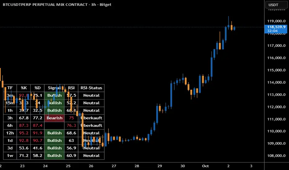
MTF Stochastic + RSI Dashboard FLEX with STRONG Alerts
A compact, multi-timeframe dashboard that shows Stochastic %K/%D, RSI and signal states across user-defined timeframes. Columns can be toggled on/off to keep the panel as small as you need. Signal texts and colors are fully customizable. The table can be placed in any chart corner, and the background color & opacity are adjustable for perfect readability.
What it shows
• For each selected timeframe: %K, %D, a signal cell (Bullish/Bearish/Strong), RSI value, and RSI state (Overbought/Oversold/Neutral).
• Timeframes are displayed as friendly labels (e.g., 60 → 1h, W → 1w, 3D → 3d).
Signals & logic
• Bullish/Bearish when %K and %D show a sufficient gap (or an optional confirmed cross).
• Strong Bullish when both %K and %D are below the “Strong Bullish max” threshold.
• Strong Bearish when both %K and %D are above the “Strong Bearish min” threshold.
• Optional confirmation: RSI < 30 for Strong Bullish, RSI > 70 for Strong Bearish.
Alerts
• Global alerts for any selected timeframes when a STRONG BULLISH or STRONG BEARISH event occurs.
Key options
• Column visibility toggles (TF, %K, %D, Signal, RSI, RSI Status).
• Custom signal texts & colors.
• Dashboard position: top-left / top-right / bottom-left / bottom-right.
• Table background color + opacity (0 = opaque, 100 = fully transparent).
• Sensitivity (minimum %K–%D gap) and optional “cross-only” mode.
• Customizable timeframes for display and for alerts.
Default settings
• Stochastic: K=5, D=3, SmoothK=3
• RSI length: 14
• Decimals: 1
• Strong Bullish max: 20
• Strong Bearish min: 80
• Default TFs & alerts: 3m, 15m, 1h, 3h, 6h, 12h, 1d, 3d, 1w
XAUUSD CSI+RSI+Delta (15m)XAUUSD 15m
Candle Stability Index: 0.4
RSI Index: 80
Candle Delta Length: 6
Disable Repeating Signals: Enabled

Oversold & Overbought Signal with RSISimple RSI overbought/oversold signals. Signals overbought when RSI > 80 and oversold when RSI < 30.

AI Trading Alerts v6 — SL/TP + Confidence + Panel (Fixed)Overview
This Pine Script is designed to identify high-probability trading opportunities in Forex, commodities, and crypto markets. It combines EMA trend filters, RSI, and Stochastic RSI, with automatic stop-loss (SL) & take-profit (TP) suggestions, and provides a confidence panel to quickly assess the trade setup strength.
It also includes TradingView alert conditions so you can set up notifications for Long/Short setups and EMA crosses.
⚙️ Features
EMA Trend Filter
Uses EMA 50, 100, 200 for trend confirmation.
Bull trend = EMA50 > EMA100 > EMA200
Bear trend = EMA50 < EMA100 < EMA200
RSI Filter
Bullish trades require RSI > 50
Bearish trades require RSI < 50
Stochastic RSI Filter
Prevents entries during overbought/oversold extremes.
Bullish entry only if %K and %D < 80
Bearish entry only if %K and %D > 20
EMA Proximity Check
Price must be near EMA50 (within ATR × adjustable multiplier).
Signals
Continuation Signals:
Long if all bullish conditions align.
Short if all bearish conditions align.
Cross Events:
Long Cross when price crosses above EMA50 in bull trend.
Short Cross when price crosses below EMA50 in bear trend.
Automatic SL/TP Suggestions
SL size adjusts depending on asset:
Gold/Silver (XAU/XAG): 5 pts
Bitcoin/Ethereum: 100 pts
FX pairs (default): 20 pts
TP = SL × Risk:Reward ratio (default 1:2).
Confidence Score (0–4)
Based on conditions met (trend, RSI, Stoch, EMA proximity).
Labels:
Strongest (4/4)
Strong (3/4)
Medium (2/4)
Low (1/4)
Visual Panel on Chart
Shows ✅/❌ for each condition (trend, RSI, Stoch, EMA proximity, signal now).
Confidence row with color-coded strength.
Alerts
Long Setup
Short Setup
Long Cross
Short Cross
🖥️ How to Use
1. Add the Script
Open TradingView → Pine Editor.
Paste the full script.
Click Add to chart.
Save as "AI Trading Alerts v6 — SL/TP + Confidence + Panel".
2. Configure Inputs
EMA Lengths: Default 50/100/200 (works well for swing trading).
RSI Length: 14 (standard).
Stochastic Length/K/D: Default 14/3/3.
Risk:Reward Ratio: Default 2.0 (can change to 1.5, 3.0, etc.).
EMA Proximity Threshold: Default 0.20 × ATR (adjust to be stricter/looser).
3. Read the Panel
Top-right of chart, you’ll see ✅ or ❌ for:
Trend → Are EMAs aligned?
RSI → Above 50 (bull) or below 50 (bear)?
Stoch OK → Not extreme?
Near EMA50 → Close enough to EMA50?
Above/Below OK → Price position vs. EMA50 matches trend?
Signal Now → Entry triggered?
Confidence row:
🟢 Green = Strongest
🟩 Light green = Strong
🟧 Orange = Medium
🟨 Yellow = Low
⬜ Gray = None
4. Alerts Setup
Go to TradingView Alerts (⏰ icon).
Choose the script under “Condition”.
Select alert type:
Long Setup
Short Setup
Long Cross
Short Cross
Set notification method (popup, sound, email, mobile).
Click Create.
Now TradingView will notify you automatically when signals appear.
5. Example Workflow
Wait for Confidence = Strong/Strongest.
Check if market session supports volatility (e.g., XAU in London/NY).
Review SL/TP suggestions:
Long → Entry: current price, SL: close - risk_pts, TP: close + risk_pts × RR.
Short → Entry: current price, SL: close + risk_pts, TP: close - risk_pts × RR.
Adjust based on your own price action analysis.
📊 Best Practices
Use on H1 + D1 combo → align higher timeframe bias with intraday entries.
Risk only 1–2% of account per trade (position sizing required).
Filter with market sessions (Asia, Europe, US).
Strongest signals work best with trending pairs (e.g., XAUUSD, USDJPY, BTCUSD).