AI Adaptive Oscillator [PhenLabs]📊 Algorithmic Adaptive Oscillator
Version: PineScript™ v6
📌 Description
The AI Adaptive Oscillator is a sophisticated technical indicator that employs ensemble learning and adaptive weighting techniques to analyze market conditions. This innovative oscillator combines multiple traditional technical indicators through an AI-driven approach that continuously evaluates and adjusts component weights based on historical performance. By integrating statistical modeling with machine learning principles, the indicator adapts to changing market dynamics, providing traders with a responsive and reliable tool for market analysis.
🚀 Points of Innovation:
Ensemble learning framework with adaptive component weighting
Performance-based scoring system using directional accuracy
Dynamic volatility-adjusted smoothing mechanism
Intelligent signal filtering with cooldown and magnitude requirements
Signal confidence levels based on multi-factor analysis
🔧 Core Components
Ensemble Framework : Combines up to five technical indicators with performance-weighted integration
Adaptive Weighting : Continuous performance evaluation with automated weight adjustment
Volatility-Based Smoothing : Adapts sensitivity based on current market volatility
Pattern Recognition : Identifies potential reversal patterns with signal qualification criteria
Dynamic Visualization : Professional color schemes with gradient intensity representation
Signal Confidence : Three-tiered confidence assessment for trading signals
🔥 Key Features
The indicator provides comprehensive market analysis through:
Multi-Component Ensemble : Integrates RSI, CCI, Stochastic, MACD, and Volume-weighted momentum
Performance Scoring : Evaluates each component based on directional prediction accuracy
Adaptive Smoothing : Automatically adjusts based on market volatility
Pattern Detection : Identifies potential reversal patterns in overbought/oversold conditions
Signal Filtering : Prevents excessive signals through cooldown periods and minimum change requirements
Confidence Assessment : Displays signal strength through intuitive confidence indicators (average, above average, excellent)
🎨 Visualization
Gradient-Filled Oscillator : Color intensity reflects strength of market movement
Clear Signal Markers : Distinct bullish and bearish pattern signals with confidence indicators
Range Visualization : Clean representation of oscillator values from -6 to 6
Zero Line : Clear demarcation between bullish and bearish territory
Customizable Colors : Color schemes that can be adjusted to match your chart style
Confidence Symbols : Intuitive display of signal confidence (no symbol, +, or ++) alongside direction markers
📖 Usage Guidelines
⚙️ Settings Guide
Color Settings
Bullish Color
Default: #2b62fa (Blue)
This setting controls the color representation for bullish movements in the oscillator. The color appears when the oscillator value is positive (above zero), with intensity indicating the strength of the bullish momentum. A brighter shade indicates stronger bullish pressure.
Bearish Color
Default: #ce9851 (Amber)
This setting determines the color representation for bearish movements in the oscillator. The color appears when the oscillator value is negative (below zero), with intensity reflecting the strength of the bearish momentum. A more saturated shade indicates stronger bearish pressure.
Signal Settings
Signal Cooldown (bars)
Default: 10
Range: 1-50
This parameter sets the minimum number of bars that must pass before a new signal of the same type can be generated. Higher values reduce signal frequency and help prevent overtrading during choppy market conditions. Lower values increase signal sensitivity but may generate more false positives.
Min Change For New Signal
Default: 1.5
Range: 0.5-3.0
This setting defines the minimum required change in oscillator value between consecutive signals of the same type. It ensures that new signals represent meaningful changes in market conditions rather than minor fluctuations. Higher values produce fewer but potentially higher-quality signals, while lower values increase signal frequency.
AI Core Settings
Base Length
Default: 14
Minimum: 2
This fundamental setting determines the primary calculation period for all technical components in the ensemble (RSI, CCI, Stochastic, etc.). It represents the lookback window for each component’s base calculation. Shorter periods create a more responsive but potentially noisier oscillator, while longer periods produce smoother signals with potential lag.
Adaptive Speed
Default: 0.1
Range: 0.01-0.3
Controls how quickly the oscillator adapts to new market conditions through its volatility-adjusted smoothing mechanism. Higher values make the oscillator more responsive to recent price action but potentially more erratic. Lower values create smoother transitions but may lag during rapid market changes. This parameter directly influences the indicator’s adaptiveness to market volatility.
Learning Lookback Period
Default: 150
Minimum: 10
Determines the historical data range used to evaluate each ensemble component’s performance and calculate adaptive weights. This setting controls how far back the AI “learns” from past performance to optimize current signals. Longer periods provide more stable weight distribution but may be slower to adapt to regime changes. Shorter periods adapt more quickly but may overreact to recent anomalies.
Ensemble Size
Default: 5
Range: 2-5
Specifies how many technical components to include in the ensemble calculation.
Understanding The Interaction Between Settings
Base Length and Learning Lookback : The base length determines the reactivity of individual components, while the lookback period determines how their weights are adjusted. These should be balanced according to your timeframe - shorter timeframes benefit from shorter base lengths, while the lookback should generally be 10-15 times the base length for optimal learning.
Adaptive Speed and Signal Cooldown : These settings control sensitivity from different angles. Increasing adaptive speed makes the oscillator more responsive, while reducing signal cooldown increases signal frequency. For conservative trading, keep adaptive speed low and cooldown high; for aggressive trading, do the opposite.
Ensemble Size and Min Change : Larger ensembles provide more stable signals, allowing for a lower minimum change threshold. Smaller ensembles might benefit from a higher threshold to filter out noise.
Understanding Signal Confidence Levels
The indicator provides three distinct confidence levels for both bullish and bearish signals:
Average Confidence (▲ or ▼) : Basic signal that meets the minimum pattern and filtering criteria. These signals indicate potential reversals but with moderate confidence in the prediction. Consider using these as initial alerts that may require additional confirmation.
Above Average Confidence (▲+ or ▼+) : Higher reliability signal with stronger underlying metrics. These signals demonstrate greater consensus among the ensemble components and/or stronger historical performance. They offer increased probability of successful reversals and can be traded with less additional confirmation.
Excellent Confidence (▲++ or ▼++) : Highest quality signals with exceptional underlying metrics. These signals show strong agreement across oscillator components, excellent historical performance, and optimal signal strength. These represent the indicator’s highest conviction trade opportunities and can be prioritized in your trading decisions.
Confidence assessment is calculated through a multi-factor analysis including:
Historical performance of ensemble components
Degree of agreement between different oscillator components
Relative strength of the signal compared to historical thresholds
✅ Best Use Cases:
Identify potential market reversals through oscillator extremes
Filter trade signals based on AI-evaluated component weights
Monitor changing market conditions through oscillator direction and intensity
Confirm trade signals from other indicators with adaptive ensemble validation
Detect early momentum shifts through pattern recognition
Prioritize trading opportunities based on signal confidence levels
Adjust position sizing according to signal confidence (larger for ++ signals, smaller for standard signals)
⚠️ Limitations
Requires sufficient historical data for accurate performance scoring
Ensemble weights may lag during dramatic market condition changes
Higher ensemble sizes require more computational resources
Performance evaluation quality depends on the learning lookback period length
Even high confidence signals should be considered within broader market context
💡 What Makes This Unique
Adaptive Intelligence : Continuously adjusts component weights based on actual performance
Ensemble Methodology : Combines strength of multiple indicators while minimizing individual weaknesses
Volatility-Adjusted Smoothing : Provides appropriate sensitivity across different market conditions
Performance-Based Learning : Utilizes historical accuracy to improve future predictions
Intelligent Signal Filtering : Reduces noise and false signals through sophisticated filtering criteria
Multi-Level Confidence Assessment : Delivers nuanced signal quality information for optimized trading decisions
🔬 How It Works
The indicator processes market data through five main components:
Ensemble Component Calculation :
Normalizes traditional indicators to consistent scale
Includes RSI, CCI, Stochastic, MACD, and volume components
Adapts based on the selected ensemble size
Performance Evaluation :
Analyzes directional accuracy of each component
Calculates continuous performance scores
Determines adaptive component weights
Oscillator Integration :
Combines weighted components into unified oscillator
Applies volatility-based adaptive smoothing
Scales final values to -6 to 6 range
Signal Generation :
Detects potential reversal patterns
Applies cooldown and magnitude filters
Generates clear visual markers for qualified signals
Confidence Assessment :
Evaluates component agreement, historical accuracy, and signal strength
Classifies signals into three confidence tiers (average, above average, excellent)
Displays intuitive confidence indicators (no symbol, +, ++) alongside direction markers
💡 Note:
The AI Adaptive Oscillator performs optimally when used with appropriate timeframe selection and complementary indicators. Its adaptive nature makes it particularly valuable during changing market conditions, where traditional fixed-weight indicators often lose effectiveness. The ensemble approach provides a more robust analysis by leveraging the collective intelligence of multiple technical methodologies. Pay special attention to the signal confidence indicators to optimize your trading decisions - excellent (++) signals often represent the most reliable trade opportunities.
Adaptive
EMA Adaptive Trailing StopThe EMA Adaptive Trailing Stop Strategy is a versatile and comprehensive Pine Script designed for TradingView. This script provides an adaptive trailing stop mechanism that leverages the Exponential Moving Average (EMA) to adjust trailing stops based on market conditions. The strategy dynamically switches between trending and ranging markets by utilizing both Average True Range (ATR) and Average Directional Index (ADX) to detect market conditions.
Key Features:
EMA-Based Trailing Stop:
The script uses the EMA value to set trailing stops precisely. The EMA offers a more responsive calculation to price changes, ensuring closer and more accurate trailing stops that follow market movements effectively.
Market Condition Detection:
The script employs ATR and ADX to distinguish between trending and ranging markets. ATR measures market volatility, while ADX gauges trend strength. The combination of these two indicators provides a more accurate market condition detection.
Customizable Settings:
The script offers various flexible parameters to adjust EMA length, multipliers, and ATR length. Users can customize these settings according to their preferences and trading strategy.
Two Modes:
The script adapts to market conditions by providing two modes: trending mode and ranging mode. In trending mode, the trailing stop is tighter to follow price movements closely, whereas in ranging mode, the trailing stop is looser to accommodate lower volatility.
Entry and Exit Conditions:
The script detects market conditions to set buy and sell signals. These conditions include the calculations of EMA, ATR, and ADX to ensure the signals generated are valid and profitable.
Alerts:
The script provides buy and sell signals through alert conditions for efficient trade management. Users can enable these alerts to get real-time notifications when valid buy or sell signals are detected.
Suitable for Scalping and Swing Trading:
The script is well-suited for both scalping and swing trading strategies. Scalpers can benefit from the responsive and tighter trailing stops during trending conditions, while swing traders can take advantage of the adaptive and looser trailing stops during ranging conditions, allowing them to capture larger price movements.
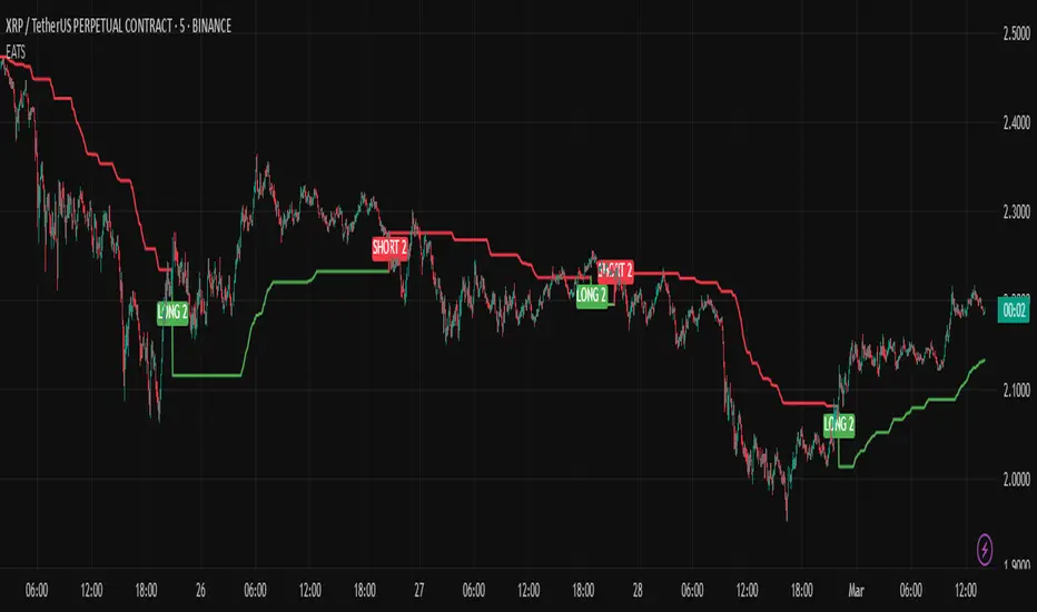
Explanation of Mode 1 and Mode 2:
Mode 1: Trending Market:
In this mode, the market is identified as trending based on the ADX and ATR values.
LONG 1: This label indicates a buy signal in the trending market mode. It signifies that the trailing stop has been activated and a long position (buy) should be taken when the market is trending.
SHORT 1: This label indicates a sell signal in the trending market mode. It signifies that the trailing stop has been activated and a short position (sell) should be taken when the market is trending.
Mode 2: Ranging Market:
In this mode, the market is identified as ranging based on the ADX and ATR values.
LONG 2: This label indicates a buy signal in the ranging market mode. It signifies that the trailing stop has been activated and a long position (buy) should be taken with a looser trailing stop when the market is ranging.
SHORT 2: This label indicates a sell signal in the ranging market mode. It signifies that the trailing stop has been activated and a short position (sell) should be taken with a looser trailing stop when the market is ranging.
Technical Usage:
Variable Initialization:
The script initializes variables to store values such as trailing stop, long position status, and short position status.
Market Condition Detection:
The script calculates ATR and ADX values to detect whether the market is trending or ranging. This includes the use of f_adx function to calculate ADX values and determine market conditions.
EMA-Based Trailing Stop Calculation:
The script adjusts the trailing stop based on EMA values and ATR. The calculation involves customizable multipliers and parameters that influence the trailing stop's precision.
Plot Trailing Stop:
The script displays the trailing stop on the chart for clear visualization. This includes plotting the trailing stop line with appropriate colors to indicate long and short positions.
Entry and Exit Conditions:
The script determines the entry (buy) and exit (sell) conditions based on market condition detection and trailing stop settings. These conditions are crucial for generating valid buy or sell signals.
Plotshape and Alert:
The script provides plotshapes for buy and sell signals and sets up alert conditions for real-time notifications when a valid buy or sell signal is detected.
Adaptive Supply and Demand [EdgeTerminal]Adaptive Supply and Demand is a dynamic supply and demand indicator with a few unique twists. It considers volume pressure, volatility-based adjustments and multi-time frame momentum for confidence scoring (multi-step confirmation) to generate dynamic lines that adjust based on the market and also to generate dynamic support/resistance levels for the supply and demand lines.
The dynamic support and resistance lines shown gives you a better situational awareness of the current state of the market and add more context to why the market is moving into a certain direction.
> Trading Scenarios
When the confidence score is over 80%, strong volume pressure in trend direction (up or down), volatility is low and momentum is aligned across timeframes, there is an indication of a strong upward or downward trend.
When the supply and demand line crossover, the confidence score is over 75% and the volume pressure is shifting, this can be an indicator of trend reversal. Use tight initial stops, scale into position as trend develops, monitor the volume pressure for continuation and wait for confidence confirmation.
When the confiance score is below 60%, the volume pressure is choppy, volatility is high, you want to avoid trading or reduce position size, wait for confidence improvements, use support and resistance for entries/exits and use tighter stops due to market conditions. This is an indication of a ranging market.
Another scenario is when there is a sudden volume pressure increase, and a raising confidence score, the volatility is expanding and the bar momentum is aligning the volatility direction. This can indicate a breakout scenario.
> How it Works
1. Volume Pressure Analysis
Volume Pressure Analysis is a key component that measures the true buying and selling force in the market. Here's a detailed breakdown. The idea is to standardize volume to prevent large spikes from skewing results.
The indicator employs an adaptive volume normalization technique to detect genuine buying and selling pressure.
It takes current volume and divides it by average volume.
If normVol > 1: Current volume is above average
If normVol < 1: Current volume is below average
An example if this would be If current volume is 1500 and average is 1000, normVol = 1.5 (50% above average)
Another component of the volume pressure analysis is the Price Change Calculation sub-module. The purpose of this is to measure price movement relative to recent average.
It works by subtracting the average price from the current price. If the value is positive, price is average and if negative, price is below average.
Finally, the volume pressure is calculated to combine volume and price for true pressure reading.
2. Savitzky-Golay Filtering
SG filtering implements advanced signal smoothing while preserving important trend features. It uses weighted moving average approximation, preserves higher moments of data and reduces noise while maintaining signal integrity.
This results in smoother signal lines, reduced false crossovers and better trend identification. Traditional moving averages tend to lag and smooth out important features. Additionally, simple moving averages can miss critical turning points and regular smoothing can delay signal generation.
SG filtering preserves higher moments such as peaks, valleys and trends, reduces noise while maintaining signal sharpness.
It works by creating a symmetric weighting scheme. This way center points get the highest weights while edge points get the lowest weight.
3. Parkinson's Volatility
Parkinson's Volatility is an advanced volatility measurement formula using high-low range data. It uses high-low range for volatility calculation, incorporates logarithmic returns and annualized the volatility measure.
This results in more accurate volatility measurement, better risk assessment and dynamic signal sensitivity.
4. Multi-timeframe Momentum
This combines signals from each module for each timeframe to calculate momentum across three timeframes. It also applies weighted importance to each timeframe and generates a composite momentum signal.
This results in a more comprehensive trend analysis, reduced timeframe bias and better trend confirmation.
> Indicator Settings
Short-term Period:
Lower values makes it more sensitive, meaning it will generate more signals. Higher values makes it less sensitive, resulting in fewer signals. We recommend a 5 to 15 range for day trading, and 10 to 20 for swing trading
Medium-term Period:
Lower values result in faster trend confirmation and higher values show slower and more reliable confirmation. We recommend a range of 15-25 for day trading and 20-30 for swing trading.
Long-term Period:
Lower values makes it more responsive to trend changes and higher values are better for major trend identification. We recommend a range of 40-60 for day trading and 50-100 for swing trading.
Volume Analysis Window:
Lower values result in more sensitivity to volume changes and higher values result in smoother volume analysis. The optimal range is 15-25 for most trading styles.
Confidence Threshold:
Lower values generate more signals but quality decreases. Higher values generate fewer signals but accuracy increases.The optimal range is 0.65-0.8 for most trading conditions.

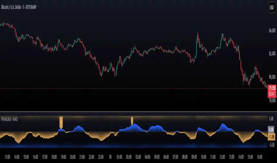
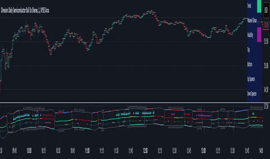
Adaptive Sharp Momentum█ Introduction
The Adaptive Sharp Momentum Study has the following all-in-one features:
• A noise-free, trend-following indicator.
• Automatically detects implied tops and bottoms within fast price cycles.
• It identifies price consolidations and periods of indecision; often challenging to spot.
• Includes a unique feature for detecting directional price squeezes.
• An integrated volatility measure helps avoid false signals and clarifies trend direction.
• Lastly, it alerts traders when a volume climax is likely reached during a move.
This study primarily focuses on capturing momentum while concurrently alerting traders to shifting market dynamics, thereby aiding in the decision to either extend a position’s duration or optimize exit timing. The set of analytical tools, deployed alongside the trend-following indicator, are integrated to reflect the concepts outlined above. Furthermore, this framework utilizes distinctive methods for trend identification, consolidation recognition, directional squeeze assessment, and volume climax analysis—approaches that are not currently documented in publicly available resources.
█ Explanation of Core Components
1. Trend Following Consolidated Adaptive Moving Average:
At the core of the study is the Jurik Adaptive Average Curve, a fast-response adaptive moving average refined with an adaptive Relative Strength Index (RSX) function, known as Jurik RSX. This curve displays three trend modes—bullish, bearish, and indecisive—each customizable in color.
Users can adjust parameters such as the Phase and Consolidation Period:
• Phase: Influences the timing of trend signals, accommodating various trading styles. A lower phase value can produce leading signals, while a higher value may result in lagging signals.
• Consolidation Period: Helps filter out false signals. Optimize this period based on the time frame and instrument.
• Momentum Slope Threshold: As mentioned earlier, the Jurik moving average values are consolidated against the Dynamic Jurik RSX. Crossing the slope threshold of the Jurik RSX will trigger consolidation.
The main curve in the middle represents the overall trend. The issue with moving averages is that they work well in trends but when market is in consolidation, many false signals can be generated. The consolidation period acts as a second fast signal curve that helps eliminate the false signals generated through the standard adaptive moving average. This is basically done by measuring the momentum of the move itself through the Jurik RSX. There are other tools in this study that should also help the trader avoid false signals which will be fully described below.
2. Implied Tops and Bottoms
The study also detects Implied Tops and Bottoms during market cycles using the Composite Momentum and Projections. It offers three detection modes:
• Strong Signals: Indicate significant potential reversal points.
• Medium Signals: Typically displayed near the end of a trend, suggesting traders should prepare to exit.
• Rolling Signals: Alert traders to set tight stop losses to secure profits, as the market may be approaching a turning point.
By default, the colors of Rolling Signals and Medium Signals are the same for simplicity.
Note the following:
• The fast and slow period have the most effect on implied tops and bottoms detection.
• Adjusting the main period will also have an overall effect.
The above chart shows rolling tops, rolling bottoms, strong tops, and strong bottoms. A rolling top of bottom indicate an increase in momentum in that direction and thus a tight stoploss would be recommended, while a strong top/bottom indicates that an exit is warranted.
3. Consolidation and Volatility
If enabled, '+' will appear above the ceiling and floor plots if consolidation is detected. Consolidation is detected by using lookback function that determine if price is below a threshold or not. If below, then consolidation would be confirmed. This is accomplished by adjusting the ' Price Consolidation Threshold ' period
The above chart demonstrates detection of consolidation on a 1-minute chart. Also, note the ceiling and floor plot, it expands when volatility is high.
Consolidation detection helps weed out long and short signals indicated by the main curve.
4. Directional Squeeze
Another unique feature of this indicator is the detection of directional price squeeze. Directional squeeze is defined as a price push in the direction indicated by momentum whether upward or downward. This is different from the common squeeze indicators found on the web since this one is detecting a directional push.
The Directional Squeeze feature, indicated by up and down triangles above the main curve, highlights strong trends in the market's current direction:
• Trend Continuation: Allows traders to stay in profitable trades longer during strong trending markets.
• Multiple Modes: Offers single-bar (short-term) and longer-term squeezes. Single-bar squeezes can signal potential market reversals, while longer-term squeezes are useful in sustained trends.
Be mindful that under certain conditions, the directional squeeze could be directionless(sideways) if consolidation is outlined by the indicator. This is another useful feature the trader could utilize. The chart above mostly demonstrates directional squeeze but directionless can also be observed.
5. Volume Volatility and Volume Climax Detection
An essential feature of the Adaptive Sharp Momentum Study is its ability to measure Volume Volatility and detect Volume Climax moments:
• Volume Volatility Measure: Integrated into the study to help avoid false signals by assessing the strength of market moves. It provides better clarity on trend direction by indicating when the market is experiencing significant volume changes.
• Volume Climax Alerts: The study alerts traders when a volume climax is likely reached during a move, which is helpful for identifying potential reversal points or the culmination of a trend. Brighter confirmation signal dots indicate these climaxes, helping traders make timely entry/exit decisions.
• Adjustable Parameters: Traders can set the Volume Volatility Threshold and adjust the Volume Lookback Period to tailor the sensitivity of volume climax detection according to their trading strategy.
5. The indicator contains other useful features:
• Cycles: Helps determine when to enter long or short trades based on upward or downward market cycles. It also aids in recognizing retracement levels during a trend, allowing traders to capitalize on brief counter-trend movements. Those cycles can be observed as the up and down gray lines on the chart.
• Real-Time Table: The table is another visual aid that summarizes the status of each feature in real-time.
█ How to Use this Study Effectively
The main curve in the middle is your final decision point. Prior to entering a trade look for the following:
• Is the market in consolidation? If yes, then you'd be advised not to enter the trade until the study clearly shows no consolidation
• Is the ceil or floor plots showing a strong top or bottom, or even a volume climax in the direction to intend to enter? If yes, then either ensure you enter at a tight stop or don't enter
• Is there an indication of a directional squeeze with no consolidation or volume climax? Then this would be an ideal place to enter. Be mindful though that entering directional squeeze too late is not recommended.
• Once you are in the trade, look at consolidation, implied tops and bottoms, and volume climax to determine exit point. You will quickly realize if you entered a trade prematurely.
• Utilize the directional squeeze and the prevalent trend to help you stay in the trade longer.
• Adjust your stop losses depending on whether you are seeing a rolling implied top/bottom or a strong top/bottom.
• Also, at volume climaxes, be ready to exit. The approach with volume climax detection should be the same as the implied tops/bottoms.
Below is a chart demonstrating trading on a 1-minute chart. The study could be used for any time frame:
** Important Note **
This study relies on volume readings. Incorrect evaluation will be concluded without proper volume data.
█ How the Adaptive Sharp Momentum Works?
---Main Curve - Jurik Moving Average and RSX---
The Jurik Moving Average (JMA) and the Jurik RSX with Fisher transform (Relative Strength Index Extended) are technical tools designed to enhance data processing efficiency. The JMA uses an adaptive smoothing algorithm to dynamically adjust to market conditions, reducing lag while maintaining high responsiveness to price changes. the JMA incorporates a mechanism that determines smoothness based on input volatility. The RSX, on the other hand, tracks relative strength without introducing the overshoots and noise commonly seen in other momentum indicators. It achieves this by applying a yet another JMA smoothing function that ensures stability and consistency, making it a better candidate for identifying shifts.
This is a unique approach, but can simply be equated to two moving averages crossing over, except in this case, the RSX is crossing over with the JMA.
The process of determining market trends and consolidation for the main curve revolves around evaluating multiple conditions and rankings of indicators such as Jurik RSX, Fisher Transform, and Volume-based metrics (Adaptive On Balance Volume and Price Volatility). Here's how consolidation and trends are identified:
1. Trend Override Logic: The core logic evaluates whether specific conditions override the default trend determined by the JMA.
• Bearish Overrides: A trend is classified as bearish if specific conditions involving negative slopes of the RSX, bearish Fisher Transform readings, and other auxiliary rankings (AOBV trend rank or volatility ranks) are met.
• Bullish Overrides: Similarly, bullish trends are determined by the presence of positive RSX slopes, bullish Fisher readings, and supporting AOBV and volatility ranks.
• Neutral Overrides: If neither bullish nor bearish overrides dominate, and conflicting conditions are detected (e.g., a bearish Fisher with a bullish OBV), the trend can be overridden to neutral.
2. Dynamic Slope and Rank Analysis: RSX and Jurik Slopes: The slopes of the RSX and Jurik indicators play an important role. Increasing slopes suggest bullish momentum, while decreasing slopes imply bearish momentum.
3. Narrow Spread Analysis: Consolidation zones are identified by examining conditions like narrow spreads in price action and mixed indicator signals (e.g., a positive RSX slope alongside a neutral or bearish AOBV).
• When consolidation is detected, the system looks for confirming signals (AOBV or Fisher alignment) to determine whether the next move is likely to be bullish or bearish.
4.Fallback Logic:
If no explicit conditions are met for bullish, bearish, or neutral trends, the system defaults to comparing the current and previous values of the Jurik Moving Average. If the JMA is rising, the trend is set to bullish; otherwise, it defaults to bearish.
The process of consolidating The RSX with JMA, attempts to confirm the trend suggested by the Jurik moving average. As shown above, several factors play into this, but it is mostly motivated by the RSX and its slope
-- Detecting Tops and Bottoms --
• Composite Momentum
The Composite Momentum indicator analyzes the market's directional strength to identify implied tops and bottoms, especially at extreme values. It evaluates momentum by categorizing it into ranges that reflect moderate or strong trends for both bullish and bearish conditions. When momentum exceeds a positive threshold, it indicates a strong top, whereas values below a negative threshold then it's a strong bottom.
• Laguerre Dynamic Projection Bands
The Laguerre Dynamic Projection Bands focuses on price positioning within calculated dynamic boundaries. By applying linear regression, it projects upper and lower price bands, which serve as potential resistance and support levels. The oscillator value ranges from 0 to 100, representing the relative position of the current price. A value above 70 indicates the price is near a projected top, while a value below 30 suggests proximity to a projected bottom. Through custom Laguerre smoothing, the setup ensures that its signals remain stable and actionable.
• How They Work Together
The Composite Momentum and Projection Oscillator complement each other in detecting market tops and bottoms. The Projection Oscillator provides an early indication when price nears a critical level, while the Composite Momentum confirms whether the momentum supports the formation of a significant top or bottom.
-- Consolidation Detection, Volatility, and Volume Climax Detection --
• Summary of Consolidation Detection:
Consolidation is identified through a combination of statistical and smoothing applied to price data. The approach calculates deviations around the main plot using squared price inputs, smoothed averages, and adaptive multipliers. These deviations form dynamic upper and lower boundaries that adapt to changing market conditions. The system further evaluates these boundaries against historical bars to calculate a volume percentage, which indicates how often recent price action remains within these bands. A low percentage suggests consolidation, characterized by reduced volatility and price movement confined within a tighter range.
The bands around the main plot are derived from the calculated maximum deviations, creating adaptive ceilings and floors that expand or contract based on market dynamics. The Ceiling and Floor plots represent the outermost boundaries, while additional retracement plots are drawn based on the Composite Momentum wave rank. For example, during an uptrend, the retrace levels adjust upward in fractional steps relative to the deviation, signaling possible resistance levels. In downtrends, similar logic applies in reverse to determine support levels. These bands visually represent the volatility envelope and help contextualize price movements relative to expected ranges. Whenever, low volatility is detected, a visual "+" indicator is added to the plot to highlight that the market is likely in consolidation mode.
• How the Adaptive OBV Applies the Same Logic:
The Adaptive On-Balance Volume (OBV) uses a similar mechanism to detect volume climaxes by analyzing deviations in volume data. Instead of price, the OBV logic applies the squared input and smoothing methods to volume flows. By comparing these deviations to historical norms, the system identifies periods of high or low volatility in volume, which often coincide with potential breakouts or consolidation zones.
• How They Work Together
The consolidation detection process and the adaptive bands work in tandem to provide traders with a clear visualization of market conditions. When consolidation is detected, the dynamic bands narrow and a "+" sign is visualized, signaling reduced volatility and potential breakout opportunities. Similarly, volume-based analysis through the adaptive OBV helps confirm whether a breakout is accompanied by significant volume, adding confidence to trade decisions. Together, they enable anticipation of market shifts.
-- Directional Squeeze --
A directional price squeeze refers to a market condition where price compresses in a particular direction. This provides traders with an opportunity to stay in trades longer by aligning with the prevailing directional bias. This unique concept generates dynamic limits based on lookback period. Their convergence upward or downward is typically a strong indication of a price push toward the respective direction.
In this approach, the system looks at the highest and lowest values of a smoothed momentum reading over a recent period and measures the distance between them. Instead of relying on a static “overbought” or “oversold” line, it calculates new boundaries as a fraction of that distance, scaling the thresholds to match the price behavior. When these dynamically adjusted limits converge, it suggests a “directional squeeze”—meaning price is moving within a more compressed or focused range. Because these boundaries adapt to the market’s own highs and lows, they provide a more responsive indication of when price may be shifting into or out of a strong directional move.
• Determining the Directional Squeeze
Directional squeeze is identified using dynamic limits derived from two key factors:
Schaff Trend Cycle (STC) for single-bar squeezes. and the Slow RSI (SRSI) for multi-bar or longer-term squeezes. Both are utilizing a custom alpha factor for adaptability and conformance with the JMA and Dynamic RSX studies.
• Directional Trend Confirmation:
If the SRSI or STC approaches the limits, additional conditions such as Fisher RSX (momentum signals) and AOBV (volume signals) and the trend already established by the JMA are aligned. If so, then a squeezed in that trend directional is established.
█ Why These Components All Work Together?
The Adaptive Sharp Momentum Study integrates multiple components to provide a framework for analyzing market dynamics. Each feature addresses specific challenges in trading:
• Core Trend Identification:
The Jurik Adaptive Moving Average (JMA) and Jurik RSX ensure better trend detection by reducing noise and dynamically confirming momentum, thus minimizing lag and false signals.
• Implied Tops and Bottoms:
The combination of Composite Momentum and Laguerre Dynamic Projection Bands highlights critical turning points. This dual-layered approach identifies potential reversals and key support/resistance levels with improved clarity.
• Consolidation and Volatility:
Adaptive ceilings, floors, and consolidation detection filter out indecisive market phases. This helps avoid unreliable signals and provides a better perspective on potential breakouts or continuations.
• Directional Squeeze:
The Directional Squeeze feature identifies directional bias in price compression. Its dynamic thresholds adapt to market conditions, aiding in the assessment of strong directional moves.
• Volume Climax:
Volume volatility and climax detection highlight key moments of market activity, aiding in the evaluation of trend strength and potential turning points.
• Integrated Framework:
The integration of these components creates a system where each element complements the others.
This study offers a methodical approach to analyzing trends, momentum, and volatility while filtering noise. It is a tool designed to assist traders in navigating complex market conditions.
█ Disclaimer
This script is provided for educational and informational purposes only and should not be considered financial advice. Trading financial instruments carries a high level of risk and may not be suitable for all investors. Before using this script, please consult with a qualified financial advisor to ensure it aligns with your individual circumstances. The author does not guarantee the accuracy or completeness of the script and is not responsible for any losses or damages that may occur from its use. Use this script at your own risk.
Adaptive On Balance Volume with Trend█ Introduction
The Adaptive On Balance Volume (AOBV) indicator enhances the traditional On Balance Volume (OBV) by introducing adaptability, volatility detection, and trend analysis. It helps traders identify the direction of volume flow, assess volume momentum, and spot potential reversals in the market.
Detecting market tops and bottoms is crucial for making informed trading decisions. The AOBV indicator offers a method for identifying these points by using an adaptive volatility detection function that highlights potential volume peaks or climaxes, suggesting when a price top or bottom may be forming.
█ Understanding the AOBV
Note: Details on how calculations are conducted can be found at the end of this script description.
1. The Basics of the AOBV Function:
• Adaptive Momentum Calculation: Instead of using a fixed momentum formula, the AOBV uses the original formula for basic momentum and enhances it based on relative strength and applies an adaptive smoothing function.
• Dynamic Smoothing:
• Strong Momentum: When the AOBV detects significant changes (strong momentum), it reduces smoothing. This makes the indicator more responsive to major market movements.
• Weak Momentum: When momentum is weak (small changes), it increases smoothing to filter out market noise.
This adaptability allows the AOBV to more accurately reflect volume momentum, responding promptly during significant market moves and remaining stable during quieter periods.
To determine the trend direction (bullish or bearish), the indicator calculates a signal curve and displays the difference as bars:
• Bar Above the Middle Line: Indicates a bullish trend.
• Bar Below the Middle Line: Indicates a bearish trend.
2. Volatility Function:
The volatility function measures how much the AOBV deviates from its average by comparing it to its smoothed version. It calculates the exponential standard deviation to estimate volatility.
• Purpose: Identifies when volume momentum is near a climax or when a trend is nearing exhaustion.
• How It Works:
• Compares current volatility to previous bars.
• Computes a percentage indicating how often the current volatility is higher than past values.
• If this percentage exceeds a defined threshold, it signals a significant volatility event by plotting a dot above or below the bar.
This pattern typically manifests itself during strong runs on price followed by a period of consolidation. Thus, estimating volatility would be an acceptable measure of when a market is reaching or nearing an implied top or bottom.
3. The Trend Function:
The trend function combines several common indicators to gauge buildup toward a reversal or a continuation of a trend when the AOBV changes direction.
• Components:
• AOBV Strength Percentage: Calculates the percentage change in the AOBV to gauge its strength and direction.
• Supertrend Indicator: Acts as the main driver for trend buildup.
• Vertical Horizontal Filter (VHF): Measures market consolidation, adjusting the trend strength accordingly.
• Adaptive RSI: Further refines the trend strength based on volume momentum.
• Trend Ranking:
• Assigns a trend rank to the AOBV that reflects both market direction and momentum.
• Colors are used to represent different trend strengths: Strong Bullish, Bullish, Strong Bearish, and Bearish.
█ How to Use the AOBV
• Above the Middle Line: Suggests a bullish trend.
• Below the Middle Line: Suggests a bearish trend
• The Volatility dots:
• Indicate strong momentum relative to previous bars.
• Signal that the trend may be nearing a climax or exhaustion.
• Can imply a potential market top or bottom.
• Consolidation can be detected by visually comparing current bars to previous ones. This should be obvious since, and as described, the AOBV bars represent volume momentum.
• The trend function is used to gauge the likelihood of a reversal or a continuation of a trend; trend is represented with several colors: strong bullish trend, bullish trend, strong bearish trend, and finally simply a bearish trend.
It is important to understand that this trend function is not the typical trend function found on other technical indicators. It must be viewed within the context of the AOBV momentum. For example, if AOBV is exerting a bullish trend (bars above middle line), then a bearish trend with no major change in momentum and no volatility indication could mean a false reversal. Conversely, a large charge in AOBV could be a strong indication of a market reversal.
█ Key Features
• Two Display Modes: Curve and Bars:
The Adaptive OBV can be viewed in two different display modes: Curve and Bars Mode. "Curve Mode" offers the classic OBV representation (but as AOBV) with trend, while "Bars Mode" incorporates volatility detection and trend, making it the recommended mode.
• Volatility Function:
• Dots appear above or below the volume bars when significant volatility events are detected.
• The sensitivity can be adjusted by changing the percentage threshold.
• Trend Analysis:
• Helps gauge the likelihood of a trend continuation or reversal.
• Uses color-coded trend ranks for easy interpretation.
• Flexible Lookback Period:
Lookback periods for the main AOBV, its signal line, trend function, and volatility function can be customized.
• Recommendations:
• Match the main lookback period with the volatility period: Ensures consistency in momentum and volatility measurements.
• Match the trend lookback period with the signal AOBV lookback period: Aligns trend analysis with the underlying momentum signals.
Below is a sample demonstrating the utility on a 1- minute chart.
█ Calculation Details:
• AOBV Calculations
The AOBV differs the traditional OBV by focusing on the differences in OBV values rather than absolute price movements. Initially, it calculates the standard OBV by accumulating volume based on whether the closing price is higher or lower than the previous close. Next, it computes the difference between the current OBV and the previous OBV to measure changes in volume momentum. It calculates the average net change and average total change of these OBV differences over a specified period using a selected averaging method (e.g., EMA, SMA). By dividing the average net change by the average total change, it obtains a change ratio that reflects the strength and direction of volume momentum.
This change ratio is then scaled to an RSI-like value between 0 and 100, which is used to derive an adaptive smoothing factor (alpha). The alpha adjusts dynamically—when the change ratio indicates strong momentum, alpha increases, making the indicator more responsive to recent changes; when momentum is weak, alpha decreases, increasing smoothing to filter out noise.
The adaptive OBV is calculated by applying this alpha to combine the current OBV and the previous adaptive OBV value. This adaptive smoothing allows the indicator to adjust its sensitivity based on market conditions, becoming more responsive during strong momentum and more stable during weak momentum.
A smoothed OBV signal line is also computed using weighted moving averages for comparison. By analyzing the difference between the adaptive OBV and this smoothed signal line, the indicator identifies bullish or bearish trends. Positive differences suggest bullish momentum (bars above the middle line), while negative differences indicate bearish momentum (bars below the middle line).
• Volatility Calculations
The volatility function in the AOBV indicator identifies significant changes in volume momentum by estimating the variability of recent momentum shifts. It begins by calculating the difference between the AOBV and its smoothed signal line, capturing the current change in volume momentum. To assess volatility, the function employs exponential smoothing to compute adaptive averages of both the volume and the squared volume over a specified lookback period. By combining these averages, it estimates the current standard deviation of the volume momentum changes, effectively measuring how much the momentum deviates from its average level.
This estimated volatility is then compared to historical volatility values over the lookback period to determine how frequently the current volatility exceeds past levels. If the proportion of times the current volatility is higher than previous values and it surpasses a user-defined threshold, it signals a significant volatility event, indicating a potential volume climax
• Trend Calculations
As outlined earlier in description, the trend function is composed of several components:
The Supertrend indicator calculates dynamic support and resistance levels based on price movements and volatility using the Average True Range. It assesses whether the closing price is above or below these levels to determine the primary trend direction. If the price is above the Supertrend line: The market is considered to be in an uptrend. If the price is below the Supertrend line: The market is considered to be in a downtrend.
The Vertical Horizontal Filter measures the strength of the trend by comparing the price range over a period to the sum of absolute price changes. It does this by comparing the difference between the highest and lowest prices over a given period (the "vertical" movement) to the sum of the absolute differences between consecutive prices (the "horizontal" movement). A higher VHF value indicates a stronger, more directional trend, while a lower value suggests that the market is moving sideways without a clear trend.. If the VHF detects consolidation, it downgrades the trend strength indicated by the Supertrend. This prevents the trend function from overemphasizing the Supertrend's signals when the market lacks clear direction.
The Adaptive RSI Analyzes recent changes in the AOBV to identify whether volume momentum is strengthening or weakening (based on the volume percent change) correlating price movement with volume momentum. It only upgrades or downgrades on a bar by bar basis if price movement is correlating with percent change. This acts as a corrective measure against the VHF since quiet periods (consolidation) can occur between strong moves. The alpha generated from the adaptive function is the same as the one generated with the AOBV calculations.
█ Disclaimer
This script is provided for educational and informational purposes only and should not be considered financial advice. Trading financial instruments carries a high level of risk and may not be suitable for all investors. Before using this script, please consult with a qualified financial advisor to ensure it aligns with your individual circumstances. The author does not guarantee the accuracy or completeness of the script and is not responsible for any losses or damages that may occur from its use. Use this script at your own risk.

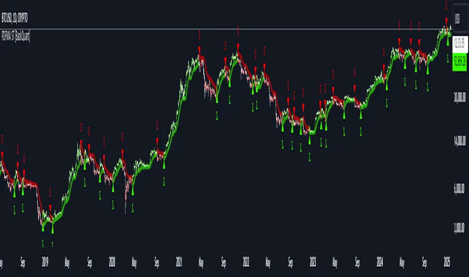
PDF-MA Supertrend [BackQuant]PDF-MA Supertrend
The PDF-MA Supertrend combines the innovative Probability Density Function (PDF) smoothing with the widely popular Supertrend methodology, creating a robust tool for identifying trends and generating actionable trading signals. This indicator is designed to provide precise entries and exits by dynamically adapting to market volatility while visualizing long and short opportunities directly on the chart.
Core Feature: PDF Smoothing
At the foundation of this indicator is the PDF smoothing technique, which applies a Probability Density Function to calculate a smoothed moving average. This method allows the indicator to assign adaptive weights to data points, making it responsive to market changes without overreacting to short-term volatility.
Key parameters include:
Variance: Controls the spread of the PDF weighting. A smaller variance results in sharper responses, while a larger variance smooths out the curve.
Mean: Shifts the PDF’s center, allowing traders to tweak how weights are distributed around the data points.
Smoothing Method: Offers the choice between EMA (Exponential Moving Average) and SMA (Simple Moving Average) for blending the PDF-smoothed data with traditional moving average methods.
By combining these parameters, the PDF smoothing creates a moving average that effectively captures underlying trends.
Supertrend: Adaptive Trend and Volatility Tracking
The Supertrend is a well-known volatility-based indicator that dynamically adjusts to market conditions using the ATR (Average True Range). In this script, the PDF-smoothed moving average acts as the price input, making the Supertrend calculation more adaptive and precise.
Key Supertrend Features:
ATR Period: Determines the lookback period for calculating market volatility.
Factor: Multiplies the ATR to set the distance between the Supertrend and the price. A higher factor creates wider bands, filtering out smaller price movements, while a lower factor captures tighter trends.
Dynamic Direction: The Supertrend flips its direction based on price interactions with the calculated upper and lower bands:
Uptrend : When the price is above the Supertrend, the direction turns bullish.
Downtrend : When the price is below the Supertrend, the direction turns bearish.
This combination of PDF smoothing and Supertrend calculation ensures that trends are detected with greater accuracy, while volatility filters out market noise.
Long and Short Signal Generation
The PDF-MA Supertrend generates actionable trading signals by detecting transitions in the trend direction:
Long Signal (𝕃): Triggered when the trend transitions from bearish to bullish. This is visually represented with a green triangle below the price bars.
Short Signal (𝕊): Triggered when the trend transitions from bullish to bearish. This is marked with a red triangle above the price bars.
These signals provide traders with clear entry and exit points, ensuring they can capitalize on emerging trends while avoiding false signals.
Customizable Visualization Options
The indicator offers a range of visualization settings to help traders interpret the data with ease:
Show Supertrend: Option to toggle the visibility of the Supertrend line.
Candle Coloring: Automatically colors candlesticks based on the trend direction:
Green for long trends.
Red for short trends.
Long and Short Signals (𝕃 + 𝕊): Displays long (𝕃) and short (𝕊) signals directly on the chart for quick identification of trade opportunities.
Line Color Customization: Allows users to customize the colors for long and short trends.
Alert Conditions
To ensure traders never miss an opportunity, the PDF-MA Supertrend includes built-in alerts for trend changes:
Long Signal Alert: Notifies when a bullish trend is identified.
Short Signal Alert: Notifies when a bearish trend is identified.
These alerts can be configured for real-time notifications via SMS, email, or push notifications, making it easier to stay updated on market movements.
Suggested Parameter Adjustments
The indicator’s effectiveness can be fine-tuned using the following guidelines:
Variance:
For low-volatility assets (e.g., indices): Use a smaller variance (1.0–1.5) for smoother trends.
For high-volatility assets (e.g., cryptocurrencies): Use a larger variance (1.5–2.0) to better capture rapid price changes.
ATR Factor:
A higher factor (e.g., 2.0) is better suited for long-term trend-following strategies.
A lower factor (e.g., 1.5) captures shorter-term trends.
Smoothing Period:
Shorter periods provide more reactive signals but may increase noise.
Longer periods offer stability and better alignment with significant trends.
Experimentation is encouraged to find the optimal settings for specific assets and trading strategies.
Trading Applications
The PDF-MA Supertrend is a versatile indicator suited to a variety of trading approaches:
Trend Following : Use the Supertrend line and signals to follow market trends and ride sustained price movements.
Reversal Trading : Spot potential trend reversals as the Supertrend flips direction.
Volatility Analysis : Adjust the ATR factor to filter out minor price fluctuations or capture sharp movements.
Final Thoughts
The PDF-MA Supertrend combines the precision of Probability Density Function smoothing with the adaptability of the Supertrend methodology, offering traders a powerful tool for identifying trends and volatility. With its customizable parameters, actionable signals, and built-in alerts, this indicator is an excellent choice for traders seeking a robust and reliable system for trend detection and entry/exit timing.
As always, backtesting and incorporating this indicator into a broader strategy are recommended for optimal results.
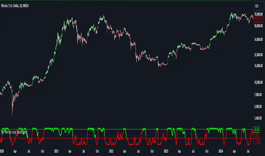
PDF MA For Loop [BackQuant]PDF MA For Loop
Introducing the PDF MA For Loop, an innovative trading indicator that combines Probability Density Function (PDF) smoothing with a dynamic for-loop scoring mechanism. This advanced tool provides traders with precise trend-following signals, helping to identify long and short opportunities with improved clarity and adaptability to market conditions.
If you would like to check out the stand alone PDF Moving Average:
Core Concept: Probability Density Function (PDF) Smoothing
The PDF smoothing method is a unique approach that applies adaptive weights to price data based on a Probability Density Function. This ensures that recent data points receive appropriate emphasis while maintaining a smooth transition across the data set. The result is a moving average that is not only smoother but also more responsive to market changes.
Key parameters in PDF smoothing:
Variance : Controls the spread of the PDF, where a higher value results in broader smoothing and a lower value makes the moving average more sensitive.
Mean : Centers the PDF around a specific value, influencing the weighting and responsiveness of the smoothing process.
By combining PDF smoothing with traditional moving averages (EMA or SMA), the indicator creates a hybrid signal that balances responsiveness and reliability.
For-Loop Scoring Mechanism
At the heart of this indicator is the for-loop scoring mechanism, which evaluates the smoothed PDF moving average over a defined range of historical data points. This process assigns a score to the current market condition based on whether the PDF moving average is greater than or less than previous values.
Long Signal: A long signal is generated when the score exceeds the Long Threshold (default set at 40), indicating upward momentum.
Short Signal: A short signal is triggered when the score crosses below the Short Threshold (default set at -10), suggesting potential downward momentum.
This dynamic scoring system ensures that the indicator remains adaptive, capturing trends and shifts in market sentiment effectively.
Customization Options
The PDF MA For Loop includes a variety of customizable settings to fit different trading styles and strategies:
Calculation Settings
Price Source : Select the input price for the calculation (default is the close price).
Smoothing Method : Choose between EMA or SMA for the additional smoothing layer, providing flexibility to adapt to market conditions.
Smoothing Period : Adjust the lookback period for the smoothing function, with shorter periods providing more sensitivity and longer periods offering greater stability.
Variance & Mean : Fine-tune the PDF function parameters to control the weighting of the smoothing process.
Signal Settings
Thresholds : Customize the upper and lower thresholds to define the sensitivity of the long and short signals.
For Loop Range : Set the range of historical data points analyzed by the for-loop, influencing the depth of the scoring mechanism.
UI Settings
Signal Line Width: Adjust the thickness of the plotted signal line for better visibility.
Candle Coloring: Enable or disable the coloring of candlesticks based on trend direction (green for long, red for short, gray for neutral).
Background Coloring: Add background shading to highlight long and short signals for an enhanced visual experience.
Alerts and Automation
The indicator includes built-in alert conditions to notify traders of important market events:
Long Signal Alert: Notifies when the score exceeds the upper threshold, indicating a bullish trend.
Short Signal Alert: Notifies when the score crosses below the lower threshold, signaling a bearish trend.
These alerts can be configured for real-time notifications, allowing traders to respond quickly to market changes without constant chart monitoring.
Trading Applications
The PDF MA For Loop is versatile and can be applied across various trading strategies and market conditions:
Trend Following: The PDF smoothing method combined with for-loop scoring makes this indicator particularly effective for identifying and following trends.
Reversal Trading: By observing the thresholds and score, traders can anticipate potential reversals when the trend shifts from long to short (or vice versa).
Risk Management: The dynamic thresholds and scoring provide clear signals, allowing traders to enter and exit trades with greater confidence and precision.
Final Thoughts
The PDF MA For Loopis merges advanced mathematical concepts with practical trading tools. By leveraging Probability Density Function smoothing and a dynamic for-loop scoring system, it provides traders with clear, actionable signals while adapting to market conditions.
Whether you’re looking for an edge in trend-following strategies or seeking precision in identifying reversals, this indicator offers the flexibility and power to enhance your trading decisions
As always, backtesting and integrating the PDF MA For Loop into a comprehensive trading strategy is recommended for optimal performance, as no single indicator should be used in isolation.
Thus following all of the key points here are some sample backtests on the 1D Chart
Disclaimer: Backtests are based off past results, and are not indicative of the future.
INDEX:BTCUSD
INDEX:ETHUSD
BINANCE:SOLUSD
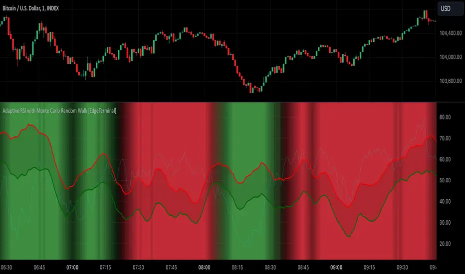
Adaptive RSI with Monte Carlo Random Walk [EdgeTerminal]The Monte Carlo Random Walk RSI indicator revolutionizes the traditional RSI by replacing static overbought/oversold levels with dynamic, statistically-driven bands that adapt to market conditions. Enhanced with smooth transitions, visual cues, and advanced filtering, this indicator provides a sophisticated approach to market analysis.
How it works:
In this indicator, the machine learning simulation works by combining multiple market signals in a weighted system that adapts to market conditions. Instead of just using simple RSI overbought/oversold levels, it analyzes the relationships between RSI, price momentum, and volatility to generate a comprehensive score.
The RSI component contributes 40% to the final signal, while momentum and volatility each contribute 30%. These signals are normalized and combined to create a score between 0-100, similar to how a machine learning model would generate probability predictions.
When this score is very high (above 80) along with traditional RSI signals, it suggests a stronger likelihood of a price reversal than using RSI alone.
The indicator doesn't use actual Monte Carlo simulations, but it does incorporate the concept of probability through its scoring system. Rather than giving simple buy/sell signals, it provides different levels of conviction (strong vs weak signals) based on how multiple factors align.
For example, a strong buy signal only occurs when both the ML score is above 80 AND the RSI is in oversold territory, indicating that multiple market conditions are favorable. This multi-factor approach helps reduce false signals that might occur with traditional RSI and provides traders with more nuanced information about potential trade opportunities.
Key Innovations:
Dynamic Bands vs Static Levels: Traditional RSI uses fixed 70/30 or 80/20 levels, this adaptive RSI creates adaptive bands based on market behavior and automatically adjusts to volatility and trend changes to reduce false signals in trending markets.
1. Calculate price volatility: σ = stdDev(returns)
2. Generate random walks: R(t) = R(t-1) + N(0,σ)
3. Transform to RSI space
4. Create probability distribution
5. Extract confidence intervals
Statistical Analysis: We use Monte Carlo simulations to generate probability bands. This allows the indicator levels to automatically adapt to current market conditions, generating more accurate overbought and oversold levels.
1. Measure deviation: D = |RSI - nearestBand|
2. Normalize by volatility: N = D/ATR
3. Calculate strength multiplier: max(1, N)
The indicator uses Monte Carlo simulations to model potential RSI paths. For each simulation, we generate random returns using market volatility, then calculate RSI components, calculate RSI, and finally, repeat N times (default 200 simulations)
Settings:
RSI Length: Controls the lookback period for the RSI calculation. Higher values result in smoother RSI, and slower signals. It affects exponential smoothing factor, impacts volatility measurement and influences random walk generation.
Number of Simulations: Controls Monte Carlo simulation count. Higher values result in more accurate bands, but lower calculation. More simulation means you get a better normal distribution, reducing random variation in bands.
Confidence Level: this controls statistical significance of bands. Higher values result in wider bands, meaning fewer trading signals are generated.
- 0.95 = 95% confidence interval
- Captures 2 standard deviations
- Controls false signal probability
Band Smoothing: Applies SMA to raw band values. Higher values mean smoother brands but result in more lag.
Minimum Signal Strength: Normalizes RSI deviation by ATR. The higher the value, it requires stronger moves. It uses ATR for volatility normalization and creates standard deviation equivalent.
Trend Sensitivity: Measures trend strength relative to volatility. Higher values filter more trending conditions
Volume Threshold: Compares current volume to average. Higher values require stronger volume confirmation. It validates price movement and confirms institutional participation.
How to Use:
Background gradually turns red in overbought and turns green in oversold conditions. Based on your trade direction, you want to pay attention when overbought or oversold levels start shifting.
For example, if you're going long on a trade, wait for oversold conditions (green) to start shifting toward red, this can indicate a move into a long direction, helping you catch the trend.
Additionally, the bands represent statistically significant levels where the RSI is likely to reverse, based on recent market behavior. The indicator runs multiple simulations of potential RSI paths. Each simulation uses recent market volatility and characteristics, then creates a statistical distribution of where RSI tends to turn around.
The Upper Band (red line) represents a statistically significant overbought level, when RSI crosses above this band and stays there for a while, the background starts to turn red, indicating it's more extended than normal. This is a lot more reliable than fixed RSI 70 level because it adapts to market conditions. Finally, the probability of reversal increases above this band. You can think of it as a dynamic overbought level.
The Lower Band (green line) is the opposite of the red line, and it represents a statistically significant oversold level. When RSI crosses below this band, it's more oversold than normal. This is a lot more reliable than fixed RSI 30 level because it adapts to market trend and the probability of reversal increases below this band.
Finally, the band width itself represents how volatile the market is. A wider band means the market is more volatile and a narrower band means the market is not as volatile. The width automatically adjusts based on market conditions.
Hybrid Adaptive Double Exponential Smoothing🙏🏻 This is HADES (Hybrid Adaptive Double Exponential Smoothing) : fully data-driven & adaptive exponential smoothing method, that gains all the necessary info directly from data in the most natural way and needs no subjective parameters & no optimizations. It gets applied to data itself -> to fit residuals & one-point forecast errors, all at O(1) algo complexity. I designed it for streaming high-frequency univariate time series data, such as medical sensor readings, orderbook data, tick charts, requests generated by a backend, etc.
The HADES method is:
fit & forecast = a + b * (1 / alpha + T - 1)
T = 0 provides in-sample fit for the current datum, and T + n provides forecast for n datapoints.
y = input time series
a = y, if no previous data exists
b = 0, if no previous data exists
otherwise:
a = alpha * y + (1 - alpha) * a
b = alpha * (a - a ) + (1 - alpha) * b
alpha = 1 / sqrt(len * 4)
len = min(ceil(exp(1 / sig)), available data)
sig = sqrt(Absolute net change in y / Sum of absolute changes in y)
For the start datapoint when both numerator and denominator are zeros, we define 0 / 0 = 1
...
The same set of operations gets applied to the data first, then to resulting fit absolute residuals to build prediction interval, and finally to absolute forecasting errors (from one-point ahead forecast) to build forecasting interval:
prediction interval = data fit +- resoduals fit * k
forecasting interval = data opf +- errors fit * k
where k = multiplier regulating intervals width, and opf = one-point forecasts calculated at each time t
...
How-to:
0) Apply to your data where it makes sense, eg. tick data;
1) Use power transform to compensate for multiplicative behavior in case it's there;
2) If you have complete data or only the data you need, like the full history of adjusted close prices: go to the next step; otherwise, guided by your goal & analysis, adjust the 'start index' setting so the calculations will start from this point;
3) Use prediction interval to detect significant deviations from the process core & make decisions according to your strategy;
4) Use one-point forecast for nowcasting;
5) Use forecasting intervals to ~ understand where the next datapoints will emerge, given the data-generating process will stay the same & lack structural breaks.
I advise k = 1 or 1.5 or 4 depending on your goal, but 1 is the most natural one.
...
Why exponential smoothing at all? Why the double one? Why adaptive? Why not Holt's method?
1) It's O(1) algo complexity & recursive nature allows it to be applied in an online fashion to high-frequency streaming data; otherwise, it makes more sense to use other methods;
2) Double exponential smoothing ensures we are taking trends into account; also, in order to model more complex time series patterns such as seasonality, we need detrended data, and this method can be used to do it;
3) The goal of adaptivity is to eliminate the window size question, in cases where it doesn't make sense to use cumulative moving typical value;
4) Holt's method creates a certain interaction between level and trend components, so its results lack symmetry and similarity with other non-recursive methods such as quantile regression or linear regression. Instead, I decided to base my work on the original double exponential smoothing method published by Rob Brown in 1956, here's the original source , it's really hard to find it online. This cool dude is considered the one who've dropped exponential smoothing to open access for the first time🤘🏻
R&D; log & explanations
If you wanna read this, you gotta know, you're taking a great responsability for this long journey, and it gonna be one hell of a trip hehe
Machine learning, apprentissage automatique, машинное обучение, digital signal processing, statistical learning, data mining, deep learning, etc., etc., etc.: all these are just artificial categories created by the local population of this wonderful world, but what really separates entities globally in the Universe is solution complexity / algorithmic complexity.
In order to get the game a lil better, it's gonna be useful to read the HTES script description first. Secondly, let me guide you through the whole R&D; process.
To discover (not to invent) the fundamental universal principle of what exponential smoothing really IS, it required the review of the whole concept, understanding that many things don't add up and don't make much sense in currently available mainstream info, and building it all from the beginning while avoiding these very basic logical & implementation flaws.
Given a complete time t, and yet, always growing time series population that can't be logically separated into subpopulations, the very first question is, 'What amount of data do we need to utilize at time t?'. Two answers: 1 and all. You can't really gain much info from 1 datum, so go for the second answer: we need the whole dataset.
So, given the sequential & incremental nature of time series, the very first and basic thing we can do on the whole dataset is to calculate a cumulative , such as cumulative moving mean or cumulative moving median.
Now we need to extend this logic to exponential smoothing, which doesn't use dataset length info directly, but all cool it can be done via a formula that quantifies the relationship between alpha (smoothing parameter) and length. The popular formulas used in mainstream are:
alpha = 1 / length
alpha = 2 / (length + 1)
The funny part starts when you realize that Cumulative Exponential Moving Averages with these 2 alpha formulas Exactly match Cumulative Moving Average and Cumulative (Linearly) Weighted Moving Average, and the same logic goes on:
alpha = 3 / (length + 1.5) , matches Cumulative Weighted Moving Average with quadratic weights, and
alpha = 4 / (length + 2) , matches Cumulative Weighted Moving Average with cubic weghts, and so on...
It all just cries in your shoulder that we need to discover another, native length->alpha formula that leverages the recursive nature of exponential smoothing, because otherwise, it doesn't make sense to use it at all, since the usual CMA and CMWA can be computed incrementally at O(1) algo complexity just as exponential smoothing.
From now on I will not mention 'cumulative' or 'linearly weighted / weighted' anymore, it's gonna be implied all the time unless stated otherwise.
What we can do is to approach the thing logically and model the response with a little help from synthetic data, a sine wave would suffice. Then we can think of relationships: Based on algo complexity from lower to higher, we have this sequence: exponential smoothing @ O(1) -> parametric statistics (mean) @ O(n) -> non-parametric statistics (50th percentile / median) @ O(n log n). Based on Initial response from slow to fast: mean -> median Based on convergence with the real expected value from slow to fast: mean (infinitely approaches it) -> median (gets it quite fast).
Based on these inputs, we need to discover such a length->alpha formula so the resulting fit will have the slowest initial response out of all 3, and have the slowest convergence with expected value out of all 3. In order to do it, we need to have some non-linear transformer in our formula (like a square root) and a couple of factors to modify the response the way we need. I ended up with this formula to meet all our requirements:
alpha = sqrt(1 / length * 2) / 2
which simplifies to:
alpha = 1 / sqrt(len * 8)
^^ as you can see on the screenshot; where the red line is median, the blue line is the mean, and the purple line is exponential smoothing with the formulas you've just seen, we've met all the requirements.
Now we just have to do the same procedure to discover the length->alpha formula but for double exponential smoothing, which models trends as well, not just level as in single exponential smoothing. For this comparison, we need to use linear regression and quantile regression instead of the mean and median.
Quantile regression requires a non-closed form solution to be solved that you can't really implement in Pine Script, but that's ok, so I made the tests using Python & sklearn:
paste.pics
^^ on this screenshot, you can see the same relationship as on the previous screenshot, but now between the responses of quantile regression & linear regression.
I followed the same logic as before for designing alpha for double exponential smoothing (also considered the initial overshoots, but that's a little detail), and ended up with this formula:
alpha = sqrt(1 / length) / 2
which simplifies to:
alpha = 1 / sqrt(len * 4)
Btw, given the pattern you see in the resulting formulas for single and double exponential smoothing, if you ever want to do triple (not Holt & Winters) exponential smoothing, you'll need len * 2 , and just len * 1 for quadruple exponential smoothing. I hope that based on this sequence, you see the hint that Maybe 4 rounds is enough.
Now since we've dealt with the length->alpha formula, we can deal with the adaptivity part.
Logically, it doesn't make sense to use a slower-than-O(1) method to generate input for an O(1) method, so it must be something universal and minimalistic: something that will help us measure consistency in our data, yet something far away from statistics and close enough to topology.
There's one perfect entity that can help us, this is fractal efficiency. The way I define fractal efficiency can be checked at the very beginning of the post, what matters is that I add a square root to the formula that is not typically added.
As explained in the description of my metric QSFS , one of the reasons for SQRT-transformed values of fractal efficiency applied in moving window mode is because they start to closely resemble normal distribution, yet with support of (0, 1). Data with this interesting property (normally distributed yet with finite support) can be modeled with the beta distribution.
Another reason is, in infinitely expanding window mode, fractal efficiency of every time series that exhibits randomness tends to infinitely approach zero, sqrt-transform kind of partially neutralizes this effect.
Yet another reason is, the square root might better reflect the dimensional inefficiency or degree of fractal complexity, since it could balance the influence of extreme deviations from the net paths.
And finally, fractals exhibit power-law scaling -> measures like length, area, or volume scale in a non-linear way. Adding a square root acknowledges this intrinsic property, while connecting our metric with the nature of fractals.
---
I suspect that, given analogies and connections with other topics in geometry, topology, fractals and most importantly positive test results of the metric, it might be that the sqrt transform is the fundamental part of fractal efficiency that should be applied by default.
Now the last part of the ballet is to convert our fractal efficiency to length value. The part about inverse proportionality is obvious: high fractal efficiency aka high consistency -> lower window size, to utilize only the last data that contain brand new information that seems to be highly reliable since we have consistency in the first place.
The non-obvious part is now we need to neutralize the side effect created by previous sqrt transform: our length values are too low, and exponentiation is the perfect candidate to fix it since translating fractal efficiency into window sizes requires something non-linear to reflect the fractal dynamics. More importantly, using exp() was the last piece that let the metric shine, any other transformations & formulas alike I've tried always had some weird results on certain data.
That exp() in the len formula was the last piece that made it all work both on synthetic and on real data.
^^ a standalone script calculating optimal dynamic window size
Omg, THAT took time to write. Comment and/or text me if you need
...
"Versace Pip-Boy, I'm a young gun coming up with no bankroll" 👻
∞
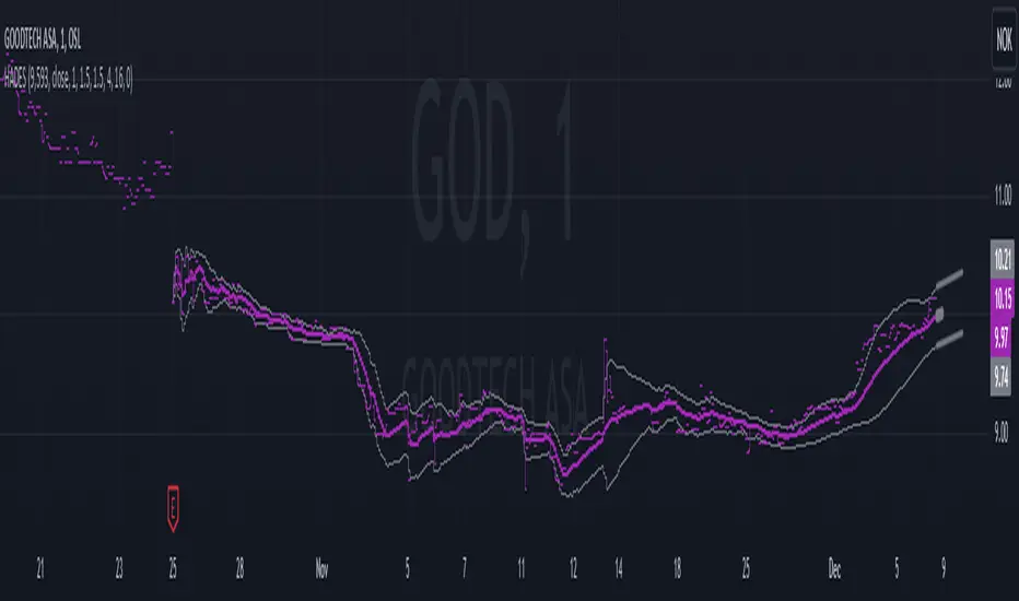
Adaptive Supertrend with Dynamic Optimization [EdgeTerminal]The Enhanced Adaptive Supertrend represents a significant evolution of the traditional Supertrend indicator, incorporating advanced mathematical optimization, dynamic volatility adjustment, intelligent signal filtering, reduced noise and false positives.
Key Features
Dynamic volatility-adjusted bands
Self-optimizing multiplier
Intelligent signal filtering system
Cooldown period to prevent signal clustering
Clear buy/sell signals with optimal positioning
Smooth trend visualization
RSI and MACD integration for confirmation
Performance-based optimization
Dynamic Band Calculation
Dynamic Band Calculation automatically adapts to market volatility, generates wider bands in volatile periods, reducing false signals. It also generates tighter bands in stable periods, capturing smaller moves and smooth transitions between different volatility regimes.
RSI Integration
The RSI and MACD play multiple crucial roles in the Adaptive Supertrend.
It first helps with momentum factor calculation. This dynamically adjusts band width based on momentum conditions. When the RSI is oversold, bands widen by 20% to prevent false signals during strong downtrends and provide more room for price movements in extreme conditions.
When the RSI is overbought, brands tighten by 20% and they become more sensitive to potential reversals to help catch trend changes earlier.
This reduces false signals in strong trends, helps detect potential reversals earlier than the usual, create adaptive band width based on market conditions and finally, better protection against whipsaws.
MACD Integration
The MACD in this supertrend indicator serves as a trend confirmation tool. The idea is to use MACD crossovers to confirm trend changes to reduce false trend change signals and enhance the signal quality.
For this to become a signal, MACD crossovers must align with price movement to help filter out weak or false signals, which acts as an additional layer of trend confirmation.
Additionally, MACD line position relative to signal line indicates trend strength, helps maintain positions in strong trends and assists in early detection of trend weakening.
Momentum Integration
Momentum Integration prevents false signals in extreme conditions, It adjusts dynamic bands based on market momentum, improves trend confirmation in strong moves and reduces whipsaws during consolidations.
Improved signals
There are a few systems to generate better signals, allowing for generally faster signals compared to original supertrend, such as:
Enforced cooldown period between signals
Prevents signal clustering
Clearer entry/exit points
Reduced false signals during choppy markets
Performance Optimization
This script implements a Sharpe ratio-inspired optimization algorithm to balance returns against risk, penalize large drawdowns, adapt parameters in real-time and improve risk-adjusted performance
Parameter Settings
ATR Period: 10 (default) - adjust based on timeframe
Initial Multiplier: 3.0 (default) - will self-optimize
Optimization Period: 50 (default) - longer periods for more stability
Smoothing Period: 3 (default) - adjust for signal smoothness
Best Practices
Use on multiple timeframes for confirmation
Allow the optimization process to run for at least 50 bars
Monitor the adaptive multiplier for trend strength indication
Consider RSI and MACD alignment for stronger signals
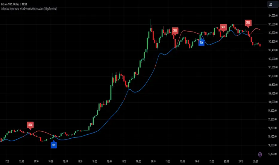
Moment-Based Adaptive DetectionMBAD (Moment-Based Adaptive Detection) : a method applicable to a wide range of purposes, like outlier or novelty detection, that requires building a sensible interval/set of thresholds. Unlike other methods that are static and rely on optimizations that inevitably lead to underfitting/overfitting, it dynamically adapts to your data distribution without any optimizations, MLE, or stuff, and provides a set of data-driven adaptive thresholds, based on closed-form solution with O(n) algo complexity.
1.5 years ago, when I was still living in Versailles at my friend's house not knowing what was gonna happen in my life tomorrow, I made a damn right decision not to give up on one idea and to actually R&D it and see what’s up. It allowed me to create this one.
The Method Explained
I’ve been wandering about z-values, why exactly 6 sigmas, why 95%? Who decided that? Why would you supersede your opinion on data? Based on what? Your ego?
Then I consciously noticed a couple of things:
1) In control theory & anomaly detection, the popular threshold is 3 sigmas (yet nobody can firmly say why xD). If your data is Laplace, 3 sigmas is not enough; you’re gonna catch too many values, so it needs a higher sigma.
2) Yet strangely, the normal distribution has kurtosis of 3, and 6 for Laplace.
3) Kurtosis is a standardized moment, a moment scaled by stdev, so it means "X amount of something measured in stdevs."
4) You generate synthetic data, you check on real data (market data in my case, I am a quant after all), and you see on both that:
lower extension = mean - standard deviation * kurtosis ≈ data minimum
upper extension = mean + standard deviation * kurtosis ≈ data maximum
Why not simply use max/min?
- Lower info gain: We're not using all info available in all data points to estimate max/min; we just pick the current higher and lower values. Lol, it’s the same as dropping exponential smoothing with alpha = 0 on stationary data & calling it a day.
You can’t update the estimates of min and max when new data arrives containing info about the matter. All you can do is just extend min and max horizontally, so you're not using new info arriving inside new data.
- Mixing order and non-order statistics is a bad idea; we're losing integrity and coherence. That's why I don't like the Hurst exponent btw (and yes, I came up with better metrics of my own).
- Max & min are not even true order statistics, unlike a percentile (finding which requires sorting, which requires multiple passes over your data). To find min or max, you just need to do one traversal over your data. Then with or without any weighting, 100th percentile will equal max. So unlike a weighted percentile, you can’t do weighted max. Then while you can always check max and min of a geometric shape, now try to calculate the 56th percentile of a pentagram hehe.
TL;DR max & min are rather topological characteristics of data, just as the difference between starting and ending points. Not much to do with statistics.
Now the second part of the ballet is to work with data asymmetry:
1) Skewness is also scaled by stdev -> so it must represent a shift from the data midrange measured in stdevs -> given asymmetric data, we can include this info in our models. Unlike kurtosis, skewness has a sign, so we add it to both thresholds:
lower extension = mean - standard deviation * kurtosis + standard deviation * skewness
upper extension = mean + standard deviation * kurtosis + standard deviation * skewness
2) Now our method will work with skewed data as well, omg, ain’t it cool?
3) Hold up, but what about 5th and 6th moments (hyperskewness & hyperkurtosis)? They should represent something meaningful as well.
4) Perhaps if extensions represent current estimated extremums, what goes beyond? Limits, beyond which we expect data not to be able to pass given the current underlying process generating the data?
When you extend this logic to higher-order moments, i.e., hyperskewness & hyperkurtosis (5th and 6th moments), they measure asymmetry and shape of distribution tails, not its core as previous moments -> makes no sense to mix 4th and 3rd moments (skewness and kurtosis) with 5th & 6th, so we get:
lower limit = mean - standard deviation * hyperkurtosis + standard deviation * hyperskewness
upper limit = mean + standard deviation * hyperkurtosis + standard deviation * hyperskewness
While extensions model your data’s natural extremums based on current info residing in the data without relying on order statistics, limits model your data's maximum possible and minimum possible values based on current info residing in your data. If a new data point trespasses limits, it means that a significant change in the data-generating process has happened, for sure, not probably—a confirmed structural break.
And finally we use time and volume weighting to include order & process intensity information in our model.
I can't stress it enough: despite the popularity of these non-weighted methods applied in mainstream open-access time series modeling, it doesn’t make ANY sense to use non-weighted calculations on time series data . Time = sequence, it matters. If you reverse your time series horizontally, your means, percentiles, whatever, will stay the same. Basically, your calculations will give the same results on different data. When you do it, you disregard the order of data that does have order naturally. Does it make any sense to you? It also concerns regressions applied on time series as well, because even despite the slope being opposite on your reversed data, the centroid (through which your regression line always comes through) will be the same. It also might concern Fourier (yes, you can do weighted Fourier) and even MA and AR models—might, because I ain’t researched it extensively yet.
I still can’t believe it’s nowhere online in open access. No chance I’m the first one who got it. It’s literally in front of everyone’s eyes for centuries—why no one tells about it?
How to use
That’s easy: can be applied to any, even non-stationary and/or heteroscedastic time series to automatically detect novelties, outliers, anomalies, structural breaks, etc. In terms of quant trading, you can try using extensions for mean reversion trades and limits for emergency exits, for example. The market-making application is kinda obvious as well.
The only parameter the model has is length, and it should NOT be optimized but picked consciously based on the process/system you’re applying it to and based on the task. However, this part is not about sharing info & an open-access instrument with the world. This is about using dem instruments to do actual business, and we can’t talk about it.
∞

Machine Learning RSI [BackQuant]Machine Learning RSI
The Machine Learning RSI is a cutting-edge trading indicator that combines the power of Relative Strength Index (RSI) with Machine Learning (ML) clustering techniques to dynamically determine overbought and oversold thresholds. This advanced indicator adapts to market conditions in real-time, offering traders a robust tool for identifying optimal entry and exit points with increased precision.
Core Concept: Relative Strength Index (RSI)
The RSI is a well-known momentum oscillator that measures the speed and change of price movements, oscillating between 0 and 100. Typically, RSI values above 70 are considered overbought, and values below 30 are considered oversold. However, static thresholds may not be effective in all market conditions.
This script enhances the RSI by integrating a dynamic thresholding system powered by Machine Learning clustering, allowing it to adapt thresholds based on historical RSI behavior and market context.
Machine Learning Clustering for Dynamic Thresholds
The Machine Learning (ML) component uses clustering to calculate dynamic thresholds for overbought and oversold levels. Instead of relying on fixed RSI levels, this indicator clusters historical RSI values into three groups using a percentile-based initialization and iterative optimization:
Cluster 1: Represents lower RSI values (typically associated with oversold conditions).
Cluster 2: Represents mid-range RSI values.
Cluster 3: Represents higher RSI values (typically associated with overbought conditions).
Dynamic thresholds are determined as follows:
Long Threshold: The upper centroid value of Cluster 3.
Short Threshold: The lower centroid value of Cluster 1.
This approach ensures that the indicator adapts to the current market regime, providing more accurate signals in volatile or trending conditions.
Smoothing Options for RSI
To further enhance the effectiveness of the RSI, this script allows traders to apply various smoothing methods to the RSI calculation, including:
Simple Moving Average (SMA)
Exponential Moving Average (EMA)
Weighted Moving Average (WMA)
Hull Moving Average (HMA)
Linear Regression (LINREG)
Double Exponential Moving Average (DEMA)
Triple Exponential Moving Average (TEMA)
Adaptive Linear Moving Average (ALMA)
T3 Moving Average
Traders can select their preferred smoothing method and adjust the smoothing period to suit their trading style and market conditions. The option to smooth the RSI reduces noise and makes the indicator more reliable for detecting trends and reversals.
Long and Short Signals
The indicator generates long and short signals based on the relationship between the RSI value and the dynamic thresholds:
Long Signals: Triggered when the RSI crosses above the long threshold, signaling bullish momentum.
Short Signals: Triggered when the RSI falls below the short threshold, signaling bearish momentum.
These signals are dynamically adjusted to reflect real-time market conditions, making them more robust than static RSI signals.
Visualization and Clustering Insights
The Machine Learning RSI provides an intuitive and visually rich interface, including:
RSI Line: Plotted in real-time, color-coded based on its position relative to the dynamic thresholds (green for long, red for short, gray for neutral).
Dynamic Threshold Lines: The script plots the long and short thresholds calculated by the ML clustering process, providing a clear visual reference for overbought and oversold levels.
Cluster Plots: Each RSI cluster is displayed with distinct colors (green, orange, and red) to give traders insights into how RSI values are grouped and how the dynamic thresholds are derived.
Customization Options
The Machine Learning RSI is highly customizable, allowing traders to tailor the indicator to their preferences:
RSI Settings : Adjust the RSI length, source price, and smoothing method to match your trading strategy.
Threshold Settings : Define the range and step size for clustering thresholds, allowing you to fine-tune the clustering process.
Optimization Settings : Control the performance memory, maximum clustering steps, and maximum data points for ML calculations to ensure optimal performance.
UI Settings : Customize the appearance of the RSI plot, dynamic thresholds, and cluster plots. Traders can also enable or disable candle coloring based on trend direction.
Alerts and Automation
To assist traders in staying on top of market movements, the script includes alert conditions for key events:
Long Signal: When the RSI crosses above the long threshold.
Short Signal: When the RSI crosses below the short threshold.
These alerts can be configured to notify traders in real-time, enabling timely decisions without constant chart monitoring.
Trading Applications
The Machine Learning RSI is versatile and can be applied to various trading strategies, including:
Trend Following: By dynamically adjusting thresholds, this indicator is effective in identifying and following trends in real-time.
Reversal Trading: The ML clustering process helps identify extreme RSI levels, offering reliable signals for reversals.
Range-Bound Trading: The dynamic thresholds adapt to market conditions, making the indicator suitable for trading in sideways markets where static thresholds often fail.
Final Thoughts
The Machine Learning RSI represents a significant advancement in RSI-based trading indicators. By integrating Machine Learning clustering techniques, this script overcomes the limitations of static thresholds, providing dynamic, adaptive signals that respond to market conditions in real-time. With its robust visualization, customizable settings, and alert capabilities, this indicator is a powerful tool for traders seeking to enhance their momentum analysis and improve decision-making.
As always, thorough backtesting and integration into a broader trading strategy are recommended to maximize the effectiveness!
Entropy-Based Adaptive SuperTrendOverview:
Introducing the Entropy-Based Adaptive SuperTrend – a groundbreaking trading indicator designed to adapt dynamically to market conditions using market entropy. This enhanced SuperTrend indicator adjusts its sensitivity according to the level of chaos (or order) in price movements, providing more stable signals during volatile periods and more responsive signals when the market becomes orderly.
Key Features:
Entropy-Adaptive Mechanism: By incorporating an entropy measure, this indicator estimates the degree of unpredictability in the market. During high entropy periods (more chaotic), signals are made less sensitive, while during low entropy periods, the indicator reacts more quickly to price changes.
Adaptive ATR Multiplier: Unlike traditional SuperTrend indicators that use a fixed ATR multiplier, this version calculates a dynamic ATR multiplier based on the entropy score, ensuring more flexibility and adaptability in setting stop levels.
Visual Clarity: The indicator is overlayed on the price chart with customizable visual elements. The bullish and bearish trends are color-coded for ease of use, and optional entry signals ("L" for long and "S" for short) are plotted to clearly mark potential entry opportunities.
Alerts for Key Opportunities : Never miss an opportunity with built-in alerts for buy and sell signals. Traders can easily configure these alerts to be notified instantly when market conditions trigger a new trend.
How It Works:
Entropy Calculation: The entropy of the price data is calculated over a user-defined period, giving an indication of the degree of randomness in the price movements. The result is then smoothed to reduce noise and create a meaningful trend indication.
Dynamic ATR Adjustment: The ATR (Average True Range) multiplier, which controls the distance of the trailing stop, is adjusted based on the entropy score. This allows the SuperTrend line to widen in chaotic times, reducing false signals, while tightening in orderly times, allowing quicker trend captures.
Parameters Explained:
Entropy Settings: Control the sensitivity of entropy calculations, including the look-back period, number of bins for price distribution, and smoothing length.
Adaptive Settings: Adjust how the indicator adapts to different levels of entropy, including the adaptation period and the filtering weight.
SuperTrend Settings : Customize the ATR period and the dynamic multiplier range to fine-tune the trailing stops for your trading style.
Visual Settings: Choose your preferred colors for bullish and bearish trends, and decide if you want the entry labels displayed directly on the chart.
Use Cases:
Swing Traders can utilize the indicator to capture trend reversals while filtering out the noise during high entropy periods.
Intraday Traders can adapt the settings for shorter time frames to benefit from dynamic adjustments that reduce overtrading and false signals.
Risk Management: The entropy-based adaptive feature provides an edge in risk management by reducing sensitivity during times of increased chaos, thus helping to limit unnecessary trades.
How to Use It:
Look for entry labels ("L" for long, "S" for short) to identify potential opportunities.
Use the color-coded trendlines to determine market bias: greenish hue for bullish trends, reddish hue for bearish trends.
Customize the input settings to align with your preferred market timeframe and risk profile.
Alerts & Notifications:
Built-in alerts notify you of significant trend changes. Simply enable these alerts to receive updates when a new long or short opportunity is detected, helping you stay ahead without needing to watch the screen constantly.
Customization Tips:
Longer Timeframes : Increase the Entropy Period to better capture macro trends in high timeframe charts.
Higher Volatility Markets: Increase the ATR Max Multiplier to ensure stops are set farther away during high entropy.
Lower Volatility Markets: Use a lower ATR Base Multiplier and tighter entropy thresholds to capture rapid price movements.
Final Thoughts:
The Entropy-Based Adaptive SuperTrend indicator merges traditional trend-following logic with an adaptive mechanism driven by market entropy, aiming to address the challenges of whipsaws and false signals common in conventional SuperTrend setups. This indicator offers an intelligent and flexible way to track market trends, suitable for both beginners and experienced trade

PDF Smoothed Moving Average [BackQuant]PDF Smoothed Moving Average
Introducing BackQuant’s PDF Smoothed Moving Average (PDF-MA) — an innovative trading indicator that applies Probability Density Function (PDF) weighting to moving averages, creating a unique, trend-following tool that offers adaptive smoothing to price movements. This advanced indicator gives traders an edge by blending PDF-weighted values with conventional moving averages, helping to capture trend shifts with enhanced clarity.
Core Concept: Probability Density Function (PDF) Smoothing
The Probability Density Function (PDF) provides a mathematical approach to applying adaptive weighting to data points based on a specified variance and mean. In the PDF-MA indicator, the PDF function is used to weight price data, adding a layer of probabilistic smoothing that enhances the detection of trend strength while reducing noise.
The PDF weights are controlled by two key parameters:
Variance: Determines the spread of the weights, where higher values spread out the weighting effect, providing broader smoothing.
Mean : Centers the weights around a particular price value, influencing the trend’s directionality and sensitivity.
These PDF weights are applied to each price point over the chosen period, creating an adaptive and smooth moving average that more closely reflects the underlying price trend.
Blending PDF with Standard Moving Averages
To further improve the PDF-MA, this indicator combines the PDF-weighted average with a traditional moving average, selected by the user as either an Exponential Moving Average (EMA) or Simple Moving Average (SMA). This blended approach leverages the strengths of each method: the responsiveness of PDF smoothing and the robustness of conventional moving averages.
Smoothing Method: Traders can choose between EMA and SMA for the additional moving average layer. The EMA is more responsive to recent prices, while the SMA provides a consistent average across the selected period.
Smoothing Period: Controls the length of the lookback period, affecting how sensitive the average is to price changes.
The result is a PDF-MA that provides a reliable trend line, reflecting both the PDF weighting and traditional moving average values, ideal for use in trend-following and momentum-based strategies.
Trend Detection and Candle Coloring
The PDF-MA includes a built-in trend detection feature that dynamically colors candles based on the direction of the smoothed moving average:
Uptrend: When the PDF-MA value is increasing, the trend is considered bullish, and candles are colored green, indicating potential buying conditions.
Downtrend: When the PDF-MA value is decreasing, the trend is considered bearish, and candles are colored red, signaling potential selling or shorting conditions.
These color-coded candles provide a quick visual reference for the trend direction, helping traders make real-time decisions based on the current market trend.
Customization and Visualization Options
This indicator offers a range of customization options, allowing traders to tailor it to their specific preferences and trading environment:
Price Source : Choose the price data for calculation, with options like close, open, high, low, or HLC3.
Variance and Mean : Fine-tune the PDF weighting parameters to control the indicator’s sensitivity and responsiveness to price data.
Smoothing Method : Select either EMA or SMA to customize the conventional moving average layer used in conjunction with the PDF.
Smoothing Period : Set the lookback period for the moving average, with a longer period providing more stability and a shorter period offering greater sensitivity.
Candle Coloring : Enable or disable candle coloring based on trend direction, providing additional clarity in identifying bullish and bearish phases.
Trading Applications
The PDF Smoothed Moving Average can be applied across various trading strategies and timeframes:
Trend Following : By smoothing price data with PDF weighting, this indicator helps traders identify long-term trends while filtering out short-term noise.
Reversal Trading : The PDF-MA’s trend coloring feature can help pinpoint potential reversal points by showing shifts in the trend direction, allowing traders to enter or exit positions at optimal moments.
Swing Trading : The PDF-MA provides a clear trend line that swing traders can use to capture intermediate price moves, following the trend direction until it shifts.
Final Thoughts
The PDF Smoothed Moving Average is a highly adaptable indicator that combines probabilistic smoothing with traditional moving averages, providing a nuanced view of market trends. By integrating PDF-based weighting with the flexibility of EMA or SMA smoothing, this indicator offers traders an advanced tool for trend analysis that adapts to changing market conditions with reduced lag and increased accuracy.
Whether you’re trading trends, reversals, or swings, the PDF-MA offers valuable insights into the direction and strength of price movements, making it a versatile addition to any trading strategy.
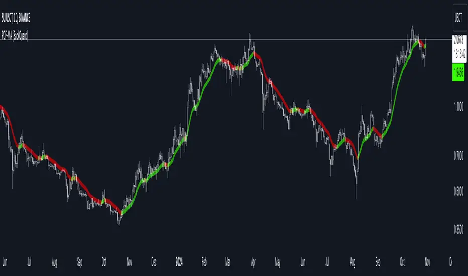
Savitzky Golay Median Filtered RSI [BackQuant]Savitzky Golay Median Filtered RSI
Introducing BackQuant's Savitzky Golay Median Filtered RSI, a cutting-edge indicator that enhances the classic Relative Strength Index (RSI) by applying both a Savitzky-Golay filter and a median filter to provide smoother and more reliable signals. This advanced approach helps reduce noise and captures true momentum trends with greater precision. Let’s break down how the indicator works, the features it offers, and how it can improve your trading strategy.
Core Concept: Relative Strength Index (RSI)
The Relative Strength Index (RSI) is a widely used momentum oscillator that measures the speed and change of price movements. It oscillates between 0 and 100, with levels above 70 typically indicating overbought conditions and levels below 30 indicating oversold conditions. However, the standard RSI can sometimes generate noisy signals, especially in volatile markets, making it challenging to identify reliable entry and exit points.
To improve upon the traditional RSI, this indicator introduces two powerful filters: the Savitzky-Golay filter and a median filter.
Savitzky-Golay Filter: Smoothing with Precision
The Savitzky-Golay filter is a digital filtering technique used to smooth data while preserving important features, such as peaks and trends. Unlike simple moving averages that can distort important price data, the Savitzky-Golay filter uses polynomial regression to fit the data, providing a more accurate and less lagging result.
In this script, the Savitzky-Golay filter is applied to the RSI values to smooth out short-term fluctuations and provide a more reliable signal. By using a window size of 5 and a polynomial degree of 2, the filter effectively reduces noise without compromising the integrity of the underlying price movements.
Median Filter: Reducing Outliers
After applying the Savitzky-Golay filter, the median filter is applied to the smoothed RSI values. The median filter is particularly effective at removing short-lived outliers, further enhancing the accuracy of the RSI by reducing the impact of sudden and temporary price spikes or drops. This combination of filters creates an ultra-smooth RSI that is better suited for detecting true market trends.
Long and Short Signals
The Savitzky Golay Median Filtered RSI generates long and short signals based on user-defined threshold levels:
Long Signals: A long signal is triggered when the filtered RSI exceeds the Long Threshold (default set at 176). This indicates that momentum is shifting upward, and it may present a good buying opportunity.
Short Signals: A short signal is generated when the filtered RSI falls below the Short Threshold (default set at 162). This suggests that momentum is weakening, potentially signaling a selling opportunity or exit from a long position.
These threshold levels can be adjusted to suit different market conditions and timeframes, allowing traders to fine-tune the sensitivity of the indicator.
Customization and Visualization Options
The Savitzky Golay Median Filtered RSI comes with several customization options, enabling traders to tailor the indicator to their specific needs:
Calculation Source: Select the price source for the RSI calculation (default is OHLC4, but it can be changed to close, open, high, or low prices).
RSI Period: Adjust the lookback period for the RSI calculation (default is 14).
Median Filter Length: Control the length of the median filter applied to the smoothed RSI, affecting how much noise is removed from the signal.
Threshold Levels: Customize the long and short thresholds to define the sensitivity for generating buy and sell signals.
UI Settings: Choose whether to display the RSI and thresholds on the chart, color the bars according to trend direction, and adjust the line width and colors used for long and short signals.
Visual Feedback: Color-Coded Signals and Thresholds
To make the signals easier to interpret, the indicator offers visual feedback by coloring the price bars and the RSI plot according to the current market trend:
Green Bars indicate long signals when momentum is bullish.
Red Bars indicate short signals when momentum is bearish.
Gray Bars indicate neutral or undecided conditions when no clear signal is present.
In addition, the Long and Short Thresholds can be plotted directly on the chart to provide a clear reference for when signals are triggered, allowing traders to visually gauge the strength of the RSI relative to its thresholds.
Alerts for Automation
For traders who prefer automated notifications, the Savitzky Golay Median Filtered RSI includes built-in alert conditions for long and short signals. You can configure these alerts to notify you when a buy or sell condition is met, ensuring you never miss a trading opportunity.
Trading Applications
This indicator is versatile and can be used in a variety of trading strategies:
Trend Following: The combination of Savitzky-Golay and median filtering makes this RSI particularly useful for identifying strong trends without being misled by short-term noise. Traders can use the long and short signals to enter trades in the direction of the prevailing trend.
Reversal Trading: By adjusting the threshold levels, traders can use this indicator to spot potential reversals. When the RSI moves from overbought to oversold levels (or vice versa), it may signal a shift in market direction.
Swing Trading: The smoothed RSI provides a clear signal for short to medium-term price movements, making it an excellent tool for swing traders looking to capitalize on momentum shifts.
Risk Management: The filtered RSI can be used as part of a broader risk management strategy, helping traders avoid false signals and stay in trades only when the momentum is strong.
Final Thoughts
The Savitzky Golay Median Filtered RSI takes the classic RSI to the next level by applying advanced smoothing techniques that reduce noise and improve signal reliability. Whether you’re a trend follower, swing trader, or reversal trader, this indicator provides a more refined approach to momentum analysis, helping you make better-informed trading decisions.
As with all indicators, it is important to backtest thoroughly and incorporate sound risk management strategies when using the Savitzky Golay Median Filtered RSI in your trading system.
Thus following all of the key points here are some sample backtests on the 1D Chart
Disclaimer: Backtests are based off past results, and are not indicative of the future.
INDEX:BTCUSD
INDEX:ETHUSD
BINANCE:SOLUSD

Adaptive Gaussian MA For Loop [BackQuant]Adaptive Gaussian MA For Loop
PLEASE Read the following carefully before applying this indicator to your trading system. Knowing the core logic behind the tools you're using allows you to integrate them into your strategy with confidence and precision.
Introducing BackQuant's Adaptive Gaussian Moving Average For Loop (AGMA FL) — a sophisticated trading indicator that merges the Gaussian Moving Average (GMA) with adaptive volatility to provide dynamic trend analysis. This unique indicator further enhances its effectiveness by utilizing a for-loop scoring mechanism to detect potential shifts in market direction. Let's dive into the components, the rationale behind them, and how this indicator can be practically applied to your trading strategies.
Understanding the Gaussian Moving Average (GMA)
The Gaussian Moving Average (GMA) is a smoothed moving average that applies Gaussian weighting to price data. Gaussian weighting gives more significance to data points near the center of the lookback window, making the GMA particularly effective at reducing noise while maintaining sensitivity to changes in price direction. In contrast to simpler moving averages like the SMA or EMA, GMA provides a more refined smoothing function, which can help traders follow the true trend in volatile markets.
In this script, the GMA is calculated over a defined Calculation Period (default 14), applying a Gaussian filter to smooth out market fluctuations and provide a clearer view of underlying trends.
Adaptive Volatility: A Dynamic Edge
The Adaptive feature in this indicator gives it the ability to adjust its sensitivity based on current market volatility. If the Adaptive option is enabled, the GMA uses a standard deviation-based volatility measure (with a default period of 20) to dynamically adjust the width of the Gaussian filter, allowing the GMA to react faster in volatile markets and more slowly in calm conditions. This dynamic nature ensures that the GMA stays relevant across different market environments.
When the Adaptive setting is disabled, the script defaults to a constant standard deviation value (default 1.0), providing a more stable but less responsive smoothing function.
Why Use Adaptive Gaussian Moving Average?
The Gaussian Moving Average already provides smoother results than standard moving averages, but by adding an adaptive component, the indicator becomes even more responsive to real-time price changes. In fast-moving or highly volatile markets, this adaptation allows traders to react quicker to emerging trends. Conversely, in quieter markets, it reduces over-sensitivity to minor fluctuations, thus lowering the risk of false signals.
For-Loop Scoring Mechanism
The heart of this indicator lies in its for-loop scoring system, which evaluates the smoothed price data (the GMA) over a specified range, comparing it to previous values. This scoring system assigns a numerical value based on whether the current GMA is higher or lower than previous values, creating a trend score.
Long Signals: These are generated when the for-loop score surpasses the Long Threshold (default set at 40), signaling that the GMA is gaining upward momentum, potentially identifying a favorable buying opportunity.
Short Signals: These are triggered when the score crosses below the Short Threshold (default set at -10), indicating that the market may be losing strength and that a selling or shorting opportunity could be emerging.
Thresholds & Customization Options
This indicator offers a high degree of flexibility, allowing you to fine-tune the settings according to your trading style and risk preferences:
Calculation Period: Adjust the lookback period for the Gaussian filter, affecting how smooth or responsive the indicator is to price changes.
Adaptive Mode: Toggle the adaptive feature on or off, allowing the GMA to dynamically adjust based on market volatility or remain consistent with a fixed standard deviation.
Volatility Settings: Control the standard deviation period for adaptive mode, fine-tuning how quickly the GMA responds to shifts in volatility.
For-Loop Settings: Modify the start and end points for the for-loop score calculation, adjusting the depth of analysis for trend signals.
Thresholds for Signals: Set custom long and short thresholds to determine when buy or sell signals should be generated.
Visualization Options: Choose to color bars based on trend direction, plot signal lines, or adjust the background color to reflect current market sentiment visually.
Trading Applications
The Adaptive Gaussian MA For Loop can be applied to a variety of trading styles and markets. Here are some key ways you can use this indicator in practice:
Trend Following: The combination of Gaussian smoothing and adaptive volatility helps traders stay on top of market trends, identifying significant momentum shifts while filtering out noise. The for-loop scoring system enhances this by providing a numerical representation of trend strength, making it easier to spot when a new trend is emerging or when an existing one is gaining strength.
Mean Reversion: For traders looking to capitalize on short-term market corrections, the adaptive nature of this indicator makes it easier to identify when price action is deviating too far from its smoothed trend, allowing for strategic entries and exits based on overbought or oversold conditions.
Swing Trading: With its ability to capture medium-term price movements while avoiding the noise of short-term fluctuations, this indicator is well-suited for swing traders who aim to profit from market reversals or short-to-mid-term trends.
Volatility Management: The adaptive feature allows the indicator to adjust dynamically in volatile markets, ensuring that it remains responsive in times of increased uncertainty while avoiding unnecessary noise in calmer periods. This makes it an effective tool for traders who want to manage risk by staying in tune with changing market conditions.
Final Thoughts
The Adaptive Gaussian MA For Loop is a powerful and flexible indicator that merges the elegance of Gaussian smoothing with the adaptability of volatility-based adjustments. By incorporating a for-loop scoring mechanism, this indicator provides traders with a comprehensive view of market trends and potential trade opportunities.
It’s important to test the settings on historical data and adapt them to your specific trading style, timeframe, and market conditions. As with any technical tool, the AGMA For Loop should be used in conjunction with other indicators and solid risk management practices for the best results.
Thus following all of the key points here are some sample backtests on the 1D Chart
Disclaimer: Backtests are based off past results, and are not indicative of the future.
INDEX:BTCUSD
INDEX:ETHUSD
BINANCE:SOLUSD

Two Pole Butterworth For Loop [BackQuant]Two Pole Butterworth For Loop
PLEASE read the following carefully, as understanding the underlying concepts and logic behind the indicator is key to incorporating it into your trading system in a sound and methodical manner.
Introducing BackQuant's Two Pole Butterworth For Loop (2P BW FL) — an advanced indicator that fuses the power of the Two Pole Butterworth filter with a dynamic for-loop scoring mechanism. This unique approach is designed to extract actionable trading signals by smoothing out price data and then analyzing it using a comparative scoring method. Let's delve into how this indicator works, why it was created, and how it can be used in various trading scenarios.
Understanding the Two Pole Butterworth Filter
The Butterworth filter is a signal processing tool known for its smooth response and minimal distortion. It's often used in electronic and communication systems to filter out unwanted noise. In trading, the Butterworth filter can be applied to price data to smooth out the volatility, providing traders with a clearer view of underlying trends without the whipsaws often associated with market noise.
The Two Pole Butterworth variant further enhances this effect by applying the filter with two poles, effectively creating a sharper transition between the passband and stopband. In simple terms, this allows the filter to follow the price action more closely, reacting to changes while maintaining smoothness.
In this script, the Two Pole Butterworth filter is applied to the Calculation Source (default is set to the closing price), creating a smoothed price series that serves as the foundation for further analysis.
Why Use a Two Pole Butterworth Filter?
The Two Pole Butterworth filter is chosen for its ability to reduce lag while maintaining a smooth output. This makes it an ideal choice for traders who want to capture trends without being misled by short-term volatility or market noise. By filtering the price data, the Two Pole Butterworth enables traders to focus on the broader market movements and avoid false signals.
The For-Loop Scoring Mechanism
In addition to the Butterworth filter, this script uses a for-loop scoring system to evaluate the smoothed price data. The for-loop compares the current value of the filtered price (referred to as "subject") to previous values over a defined range (set by the start and end input). The score is calculated based on whether the subject is higher or lower than the previous points, and the cumulative score is used to determine the strength of the trend.
Long and Short Signal Logic
Long Signals: A long signal is triggered when the score surpasses the Long Threshold (default set at 40). This suggests that the price has built sufficient upward momentum, indicating a potential buying opportunity.
Short Signals: A short signal is triggered when the score crosses under the Short Threshold (default set at -10). This indicates weakening price action or a potential downtrend, signaling a possible selling or shorting opportunity.
By utilizing this scoring system, the indicator identifies moments when the price momentum is shifting, helping traders enter positions at opportune times.
Customization and Visualization Options
One of the strengths of this indicator is its flexibility. Traders can customize various settings to fit their personal trading style or adapt it to different markets and timeframes:
Calculation Periods: Adjust the lookback period for the Butterworth filter, allowing for shorter or longer smoothing depending on the desired sensitivity.
Threshold Levels: Set the long and short thresholds to define when signals should be triggered, giving you control over the balance between sensitivity and specificity.
Signal Line Width and Colors: Customize the visual presentation of the indicator on the chart, including the width of the signal line and the colors used for long and short conditions.
Candlestick and Background Colors: If desired, the indicator can color the candlesticks or the background according to the detected trend, offering additional clarity at a glance.
Trading Applications
This Two Pole Butterworth For Loop indicator is versatile and can be adapted to various market conditions and trading strategies. Here are a few use cases where this indicator shines:
Trend Following: The Butterworth filter smooths the price data, making it easier to follow trends and identify when they are gaining or losing strength. The for-loop scoring system enhances this by providing a clear indication of how strong the current trend is compared to recent history.
Mean Reversion: For traders looking to identify potential reversals, the indicator’s ability to compare the filtered price to previous values over a range of periods allows it to spot moments when the trend may be losing steam, potentially signaling a reversal.
Swing Trading: The combination of smoothing and scoring allows swing traders to capture short to medium-term price movements by filtering out the noise and focusing on significant shifts in momentum.
Risk Management: By providing clear long and short signals, this indicator helps traders manage their risk by offering well-defined entry and exit points. The smooth nature of the Butterworth filter also reduces the risk of getting caught in false signals due to market noise.
Final Thoughts
The Two Pole Butterworth For Loop indicator offers traders a powerful combination of smoothing and scoring to detect meaningful trends and shifts in price momentum. Whether you are a trend follower, swing trader, or someone looking to refine your entry and exit points, this indicator provides the tools to make more informed trading decisions.
As always, it's essential to backtest the indicator on historical data and tailor the settings to your specific trading style and market. While the Butterworth filter helps reduce noise and smooth trends, no indicator can predict the future with absolute certainty, so it should be used in conjunction with other tools and sound risk management practices.
Thus following all of the key points here are some sample backtests on the 1D Chart
Disclaimer: Backtests are based off past results, and are not indicative of the future.
INDEX:BTCUSD
INDEX:ETHUSD
BINANCE:SOLUSD

Kalman PSaR [BackQuant]Kalman PSaR
Overview and Innovation
The Kalman PSaR combines the well-known Parabolic SAR (PSaR) with the advanced smoothing capabilities of the Kalman Filter . This innovative tool aims to enhance the traditional PSaR by integrating Kalman filtering, which reduces noise and improves trend detection. The Kalman PSaR adapts dynamically to price movements, making it a highly effective indicator for spotting trend shifts while minimizing the impact of false signals caused by market volatility.
Please Find the Basic Kalman Here:
Kalman Filter Dynamics
The Kalman Filter is a powerful algorithm for estimating the true value of a system amidst noisy data. In the Kalman PSaR, this filter is applied to the high, low, and closing prices, resulting in a smoother and more accurate representation of price action. The filter’s parameters—process noise and measurement noise—are customizable, allowing traders to fine-tune the sensitivity of the indicator to market conditions. By reducing the impact of noise, the Kalman-filtered PSaR offers clearer signals for identifying trend reversals and continuations.
Enhanced PSaR Calculation
The traditional Parabolic SAR is a popular trend-following indicator that highlights potential entry and exit points based on price acceleration. In the Kalman PSaR, this calculation is enhanced by the Kalman-filtered prices, providing a smoother and more reliable signal. The indicator continuously updates based on the acceleration factor and max step values, while the Kalman filter ensures that sudden price spikes or market noise do not trigger false signals.
Min Step and Max Step: These settings control the sensitivity of the PSaR. The Min Step sets the initial acceleration factor, while the Max Step limits how fast the PSaR adapts to price changes, helping traders fine-tune the indicator’s responsiveness.
Optional Smoothing Techniques To further enhance the signal clarity, the Kalman PSaR includes an optional smoothing feature. Traders can choose from various smoothing methods, such as SMA, Hull, EMA, WMA, TEMA, and more, to reduce short-term fluctuations and emphasize the underlying trend. The smoothing period is customizable, allowing traders to adjust the indicator’s behavior according to their preferred trading style and timeframe.
Color-Coded Candle Painting The Kalman PSaR features color-coded candles that change according to the trend direction. When the price is above the PSaR, candles are painted green to indicate a long trend, and when the price is below the PSaR, candles are painted red to signal a short trend. This visual representation makes it easy to interpret market sentiment at a glance, improving decision-making speed during fast-moving markets.
Key Features and Customization
Kalman Filter Customization: The process noise and measurement noise parameters allow traders to adjust how aggressively the filter adapts to price changes, making it suitable for both volatile and stable markets.
Smoothing Options: A variety of moving average types, such as SMA, Hull, EMA, and more, can be applied to smooth the PSaR values, ensuring that the signal remains clear even in choppy markets.
Dynamic Trend Detection: The Kalman PSaR dynamically updates based on price movements, helping traders spot trend reversals early while filtering out false signals caused by short-term volatility.
Bar Coloring and PSaR Plotting: Traders can choose to color candles based on trend direction or plot the PSaR directly on the chart for additional visual clarity.
Practical Applications
Trend-Following Strategies: The Kalman PSaR excels in trend-following strategies by providing timely signals of trend changes. The dynamic nature of the indicator allows traders to capture significant price movements while avoiding market noise.
Reversal Identification: The indicator’s ability to filter out noise and provide smoother signals makes it ideal for identifying reversals in volatile markets.
Risk Management: By plotting clear stop levels based on the PSaR, traders can use this indicator to effectively manage risk, placing stop-loss orders at key points based on the trend direction.
Conclusion
The Kalman PSaR is a fusion of the classic Parabolic SAR and the Kalman filter, offering enhanced trend detection with reduced noise. Its customizable filtering and smoothing options, combined with dynamic trend-following capabilities, make it a versatile tool for traders seeking to improve their timing and signal accuracy. The adaptive nature of the Kalman filter, combined with the robust PSaR logic, helps traders stay on the right side of the market and manage risk more effectively.

Fisher Divergence Overlay [BackQuant]Fisher Divergence Overlay
You can find the other Fisher Script Here !
Overlay Adaptation The Fisher Divergence Overlay is a newly enhanced version of the original Fisher Transformation indicator, designed specifically to be plotted directly on price charts. This adaptation allows traders to visualize Fisher Transform signals, divergences, and trend shifts directly over the price action, offering a more intuitive way to monitor market trends and potential reversals without the need for separate indicator windows. The overlay structure is particularly useful for spotting divergences and shifts in momentum as they relate to key price levels.
Why Turn the Fisher into an Overlay?
By transforming the Fisher Divergence indicator into an overlay, traders gain a more direct view of the relationship between price movements and the Fisher Transformation's signals. Divergences and midline crossovers, key components of the Fisher strategy, can now be clearly seen relative to the current price action. The decision to integrate this functionality as an overlay allows for a cleaner and more insightful trading experience, helping traders make quicker, more informed decisions based on market dynamics.
Midline Cross Signals : The overlay makes it easy to see when the Fisher Transform crosses above or below the midline, a critical signal for potential trend reversals.
Divergence Signals : Both regular and hidden divergences are plotted directly over price bars, offering immediate visual confirmation of potential trend shifts.
Key Features of the Overlay Version
Kaufman Adaptive Moving Average (KAMA): The Fisher Transformation in this overlay version can be adapted using Kaufman’s Adaptive Moving Average (KAMA). This enhances the Fisher's responsiveness to current market volatility, smoothing out price data while maintaining the accuracy of trend signals.
Divergence Detection: The overlay includes both regular and hidden bullish and bearish divergence detection, with these divergences plotted directly on the price chart. This visual feedback makes it easier for traders to spot when the momentum of the Fisher Transform deviates from the actual price movement, often signaling potential reversals.
Dynamic Bar Coloring: The bars are color-coded based on either the Fisher trend or divergences, allowing traders to visually interpret market sentiment without additional analysis. Green bars signal an upward trend or bullish divergence, while red bars indicate a downward trend or bearish divergence.
Take Profit Hues: In conjunction with a normalized RSI, the overlay includes background hues for overbought and oversold conditions, providing additional context for exit points or potential reversals.
How to Use the Fisher Overlay Traders can use this overlay to streamline their workflow by having both the Fisher signals and price action in the same visual space. The key signals include:
Midline Cross Signals: A crossover of the Fisher Transform above the midline often indicates a shift toward bullish momentum, while a cross below suggests bearish momentum.
Divergences: Regular and hidden divergences, displayed directly on the chart, help traders identify moments when the momentum of the Fisher Transform is in contrast with price movements, signaling potential reversals.
RSI Confluence: Overbought and oversold signals, provided by the integrated RSI, give further insight into potential exhaustion points in the market, marked by background color changes on the chart.
Strategic Value of the Fisher Divergence Overlay
This overlay offers a streamlined, efficient way to interpret Fisher Transform signals, divergences, and confluence signals like RSI in real-time. The visual integration of these signals with price action enhances decision-making by providing immediate context, making it easier to spot high-probability trade setups.
Trend Confirmation: The overlay version helps confirm trends by visually aligning Fisher Transform signals with price levels. Traders can use this feature to strengthen their conviction before entering or exiting a trade.
Adaptability: With the option to use KAMA for adaptive price smoothing, this overlay remains responsive across different market environments, making it suitable for both trending and volatile markets.
Summary and Interpretation Tips
It enhances the traditional Fisher Transform with visual elements like divergence detection, RSI confluence, and midline cross signals. By overlaying these elements directly on the price chart, traders can quickly interpret key signals and make better trading decisions.
Use this indicator to identify trend shifts and potential reversals by focusing on midline crossovers and divergences. The visual cues—bar colors, divergence labels, and background hues—make it easy to spot actionable moments without cluttering the chart. For best results, combine this overlay with other trend-following tools to confirm your trades and maximize the utility of Fisher Transform signals.

Multi-Kernel CCI [BackQuant]Multi-Kernel CCI
Conceptual Foundation and Innovation
It offers a fresh take on the Commodity Channel Index (CCI) by integrating three distinct kernel functions—Exponential Decay, Gaussian Decay, and Cosine Decay—to create a more robust and adaptive momentum indicator. The use of these kernel functions allows the CCI calculation to be more responsive to price changes while smoothing out noise, providing traders with clearer trend signals and reducing false alerts in varying market conditions.
Technical Composition and Calculation
The core of this indicator is a multi-kernel approach to calculating the CCI, where three different decay kernels are applied to the price source. Each kernel provides a unique weighting mechanism for price data over a user-defined lookback period. The result is an average of these three kernel calculations, which serves as the foundation for the CCI calculation. This innovative approach makes the Multi-Kernel CCI more adaptive to different market conditions compared to traditional CCI calculations.
Exponential Decay Kernel: Applies an exponential weighting to recent price data, giving more importance to recent values while smoothing out older data.
Gaussian Decay Kernel: Weights data using a Gaussian function, ensuring smooth transitions between price points and reducing outliers' impact.
Cosine Decay Kernel: Utilizes a cosine function to apply a unique oscillating weight to the data, capturing cyclical market movements more effectively.
Adaptive Thresholding: Like the Adaptive Momentum Oscillator, this indicator adjusts its long and short thresholds dynamically using percentile-based calculations over historical CCI values.
Features and User Inputs The Multi-Kernel CCI offers a wide range of customization options for traders:
Kernel Calculation Length & Alpha: Traders can fine-tune the sensitivity of the CCI by adjusting the length of the kernel calculation and the alpha parameter for the Exponential Decay Kernel.
Adaptive Thresholds: The indicator provides percentile-based thresholds for both long and short signals, allowing traders to dynamically adjust their signals based on historical data.
Extreme Value Detection: This feature highlights extreme overbought and oversold conditions with customizable thresholds and background hues, visually aiding in identifying high-probability reversal zones.
Divergence Detection: The script includes a divergence detection feature, identifying regular and hidden bullish or bearish divergences to help traders spot potential trend reversals.
Practical Applications The Multi-Kernel CCI excels in markets where adaptive trend detection and momentum confirmation are critical. Traders can leverage this tool in several ways:
Adaptive Trend Following: The dynamically adjusting thresholds allow traders to capture trends more effectively while avoiding false signals during consolidations or choppy markets.
Reversal Detection: The multi-kernel approach ensures that reversals are detected with greater precision, particularly in volatile markets where traditional indicators might fail.
Divergence Identification: With built-in divergence detection, the indicator provides traders with an early warning of potential trend reversals, helping to time their entries and exits more effectively.
Advantages and Strategic Value The Multi-Kernel CCI offers several strategic advantages over traditional CCI indicators:
Multi-Kernel Smoothing:
By using multiple decay kernels, this CCI calculation is better suited to detect subtle changes in market momentum, reducing the impact of noise and providing clearer trend signals.
Dynamic Thresholds:
The adaptive percentile-based thresholds ensure that the indicator remains relevant across different market conditions, enhancing signal accuracy.
Visual and Analytical Aids:
With features like extreme value detection and divergence spotting, this indicator equips traders with powerful tools to confirm trend strength and identify potential reversals.
Summary and Usage Tips
The Multi-Kernel CCI is a highly versatile tool for traders seeking a more adaptive and robust momentum indicator. Its multi-kernel foundation provides smoother, more reliable signals, while the adaptive thresholds and divergence detection features help traders refine their entries and exits. The dynamic nature of this indicator makes it ideal for both trend-following and reversal strategies in volatile markets.
Traders should experiment with the kernel calculation length and alpha parameter to align the indicator's sensitivity with their specific trading style and market conditions. Additionally, the adaptive thresholds can be fine-tuned to ensure the CCI captures the most significant trend changes without being overly reactive to short-term fluctuations.
Thus following all of the key points here are some sample backtests on the 1D Chart
Disclaimer: Backtests are based off past results, and are not indicative of the future.
INDEX:BTCUSD
INDEX:ETHUSD
BINANCE:SOLUSD
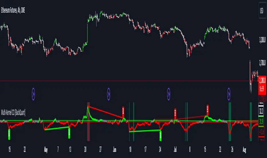
Kalman Filter RoC with Adaptive Thresholds [BackQuant]Kalman Filter RoC with Adaptive Thresholds
Another Kalman Script !!
Please Find the Basic Kalman Here:
Overview and Purpose
The Kalman Filter RoC with Adaptive Thresholds is an advanced tool designed for traders seeking to refine their trend detection and momentum analysis. By combining the robustness of the Kalman filter with the Rate of Change (RoC) indicator, this tool offers a highly responsive and adaptive method to identify shifts in market trends. The inclusion of adaptive thresholding further enhances the indicator’s precision by dynamically adjusting to market volatility, providing traders with reliable entry and exit signals.
Kalman Filter Dynamics
The Kalman Filter is renowned for its ability to estimate the true state of a system amidst noisy data. In this indicator, the Kalman filter is applied to the price data to smooth out fluctuations and generate a more accurate representation of the underlying trend. This is particularly useful in volatile markets where noise can obscure the true direction of price movements. The Kalman filter adapts in real-time based on user-defined parameters, such as process noise and measurement noise, making it highly customizable for different market conditions.
Rate of Change (RoC) and Smoothing The Rate of Change (RoC) is a classic momentum indicator that measures the percentage change in price over a specific period. By integrating it with the Kalman-filtered price, the RoC becomes more responsive to genuine price trends while filtering out short-term noise. An optional smoothing feature using the ALMA (Arnaud Legoux Moving Average) further refines the signal, allowing traders to adjust the calculation length and smoothing factor (sigma) for even greater precision.
Adaptive Thresholds A key innovation in this indicator is the adaptive thresholding mechanism. Traditional RoC indicators rely on static thresholds to identify overbought or oversold conditions, but the Kalman Filter RoC adapts these thresholds dynamically. The adaptive thresholds are calculated based on the historical volatility of the filtered RoC values, allowing the indicator to adjust in response to changing market conditions. This feature reduces the risk of false signals in choppy or highly volatile markets.
Divergence Detection The Kalman Filter RoC also includes divergence detection, helping traders identify when the momentum of the RoC diverges from the price action. Divergences can often signal potential reversals or trend continuations, making them a valuable tool in any trader’s toolkit. Regular and hidden divergences are plotted directly on the chart, providing visual cues for traders to act upon.
Customization and Flexibility This indicator offers a wide range of customization options, making it suitable for various trading strategies and market conditions:
Process Noise & Measurement Noise: These parameters control how sensitive the Kalman filter is to price changes and help traders fine-tune the balance between noise reduction and signal responsiveness.
ALMA Smoothing: Traders can apply ALMA smoothing to the RoC signal to reduce short-term volatility and improve signal clarity.
Adaptive Threshold Calculation Period: The length of the lookback period for the adaptive thresholds can be adjusted, allowing traders to tailor the indicator to fit their specific trading style.
Practical Applications
Trend Detection: The Kalman-filtered RoC helps identify shifts in momentum, making it easier for traders to spot emerging trends early. The dynamic thresholding ensures that these signals are reliable, even in volatile markets.
Divergence Trading: Divergences between the RoC and price action are clear indicators of potential trend reversals. The visual plotting of divergences simplifies the process of identifying these opportunities.
Momentum Analysis: The combination of Kalman filtering and RoC provides a smoother, more accurate view of market momentum, helping traders stay on the right side of the market.
Conclusion
The Kalman Filter RoC is a powerful and adaptable tool that merges advanced filtering techniques with momentum analysis. Its real-time responsiveness and dynamic thresholding make it a highly effective indicator for identifying trends, managing risk, and capitalizing on divergence signals. Traders looking to enhance their trend-following or momentum strategies will find this indicator to be a valuable addition to their toolkit.
Thus following all of the key points here are some sample backtests on the 1D Chart
Disclaimer: Backtests are based off past results, and are not indicative of the future.
INDEX:BTCUSD
INDEX:ETHUSD
BINANCE:SOLUSD

DEMA Adaptive DMI [BackQuant]DEMA Adaptive DMI
PLEASE Read the following, knowing what an indicator does at its core before adding it into a system is pivotal. The core concepts can allow you to include it in a logical and sound manner.
Conceptual Foundation and Innovation
The DEMA Adaptive DMI blends the Double Exponential Moving Average (DEMA) with the Directional Movement Index (DMI) to offer a unique approach to trend-following. By applying DEMA to the high and low prices, this indicator refines the traditional DMI calculation, enhancing its responsiveness to price changes. This results in a more adaptive and timely measure of market trends and momentum, providing traders with a more refined tool for capturing directional movements in the market.
Technical Composition and Calculation
At its core, the DEMA Adaptive DMI calculates the DEMA for both the high and low prices over a user-defined period. This dual application of DEMA serves to smooth out price fluctuations while retaining sensitivity to market movements. The DMI is then derived from the changes in these DEMA values, producing a set of plus and minus directional indicators that reflect the prevailing trend. Additionally, an Average Directional Index (ADX) is computed to measure the strength of the trend, with the entire process being dynamically adjusted based on the DEMA calculations.
DEMA Application:
The DEMA is applied to both high and low prices to reduce lag and provide a smoother representation of price action.
Directional Movement Calculation: The DMI is calculated using the smoothed price changes, resulting in plus and minus indicators that accurately reflect market trends.
ADX Calculation:
The ADX is computed to quantify the strength of the trend, offering traders insight into whether the market is trending strongly or is in a phase of consolidation.
Features and User Inputs The DEMA Adaptive DMI offers a range of customizable options to suit different trading styles and market conditions:
DEMA Calculation Period: Users can set the period for the DEMA calculation, allowing for adjustments based on the desired sensitivity.
DMI Length: The length of the DMI calculation can be adjusted, providing flexibility in how trends are measured.
ADX Smoothing Period: The smoothing period for the ADX can be customized to fine-tune the trend strength measurement.
Divergence Detection: Optional divergence detection features allow traders to spot potential reversals based on the DMI and price action.
Visualization options include static high and low levels to mark extreme DMI thresholds, the ability to color bars according to trend direction, and background hues to highlight overbought and oversold conditions.
Practical Applications
The DEMA Adaptive DMI is particularly effective in markets where trend strength and direction are crucial for successful trading. Traders can leverage this indicator to:
Identify Trend Reversals:
Detect potential trend reversals by monitoring the DMI and ADX in conjunction with divergence signals.
Trend Confirmation:
Use the DEMA-based DMI to confirm the strength and direction of a trend, aiding in the timing of entries and exits.
Strategic Positioning:
The indicator's responsiveness allows traders to position themselves effectively in fast-moving markets, reducing the risk of late entries or exits.
Advantages and Strategic Value
By integrating the DEMA with the DMI, this indicator provides a more adaptive and timely measure of market trends. The reduced lag from the DEMA ensures that traders receive signals that are closely aligned with current market conditions, while the dynamic DMI calculation offers a more accurate representation of trend direction and strength. This makes the DEMA Adaptive DMI a valuable tool for traders looking to enhance their trend-following strategies with a focus on precision and adaptability.
Summary and Usage Tips
The DEMA Adaptive DMI is a sophisticated trend-following indicator that combines the benefits of DEMA and DMI into a single, powerful tool. Traders are encouraged to incorporate this indicator into their trading systems for a more nuanced and responsive approach to trend detection and confirmation. Whether used for identifying trend reversals, confirming trend strength, or strategically positioning in the market, the DEMA Adaptive DMI offers a versatile and reliable solution for trend-following strategies.
Thus following all of the key points here are some sample backtests on the 1D Chart
Disclaimer: Backtests are based off past results, and are not indicative of the future.
INDEX:BTCUSD
INDEX:ETHUSD
BINANCE:SOLUSD

Adaptive RSI BandsThe RSI Band Optimizer is an innovative technical analysis tool designed to identify and display the most effective Relative Strength Index (RSI) band values for any given trading instrument. This powerful indicator dynamically calculates optimal overbought and oversold levels, moving beyond the traditional static 70/30 or 80/20 bands.
Core Functionality:
Dynamic RSI Band Calculation:
The indicator analyzes historical price data to determine the most effective RSI levels for identifying overbought and oversold conditions specific to the current trading instrument and timeframe.
Adaptive Optimization:
Rather than relying on external factors, the tool uses a proprietary algorithm that focuses solely on the relationship between historical RSI values and subsequent price movements. This pure RSI-based approach ensures that the bands are optimized for the indicator's own dynamics.
Continuous Recalibration:
The optimal RSI bands are continuously recalculated as new price data becomes available, ensuring that the indicator adapts to changing market conditions and remains relevant over time.
Key Inputs:
RSI Length:
Allows users to set the period for the RSI calculation. While the default is typically 14, users can adjust this to suit their trading style and the characteristics of the instrument they're trading.
Optimization Lookback:
Defines the historical period the indicator uses to calculate optimal bands. This balance between recent market behavior and longer-term patterns.
Band Sensitivity:
Enables fine-tuning of how aggressively the indicator adjusts the RSI bands. Higher sensitivity results in more frequent band adjustments, while lower sensitivity provides more stable levels.
What Makes It Unique:
Self-Contained Optimization:
Unlike indicators that rely on external data sources or comparisons, this tool focuses purely on optimizing RSI bands based on the indicator's own historical performance.
Instrument-Specific Bands:
By calculating optimal bands for each specific instrument, the indicator acknowledges that different assets may have different typical RSI ranges and behaviors.
Timeframe Adaptability:
The optimization process adapts to the selected timeframe, recognizing that optimal RSI bands may differ between short-term and long-term charts.
Dynamic Band Adjustment:
The continuous recalibration of bands allows the indicator to adapt to changing market volatility and trends, providing more relevant signals over time.
Enhanced RSI Interpretation:
By providing optimized, asset-specific overbought and oversold levels, the indicator offers a more nuanced and potentially more accurate interpretation of RSI values.
The RSI Band Optimizer represents a significant advancement in the application of the Relative Strength Index. By dynamically calculating optimal band values, it addresses one of the main criticisms of traditional RSI usage – the reliance on static, one-size-fits-all overbought and oversold levels. This tool empowers traders to make more informed decisions based on RSI readings that are truly tailored to the specific characteristics of the asset they're trading.