FUNCTION: Goertzel algorithm -- DFT of a specific frequency binThis function implements the Goertzel algorithm (for integer N).
The Goertzel algorithm is a technique in digital signal processing (DSP) for efficient evaluation of the individual terms of the discrete Fourier transform (DFT).
In short, it measure the power of a specific frequency like one bin of a DFT, over a rolling window (N) of samples.
Here you see an input signal that changes frequency and amplitude (from 7 bars to 17). I am running the indicator 3 times to show it measuring both frequencies and one in between (13). You can see it very accurately measures the signals present and their power, but is noisy in the transition. Changing the block len will cause it to be more responsive but noisier.
Here is a picture of the same signal, but with white noise added.
If you have a cycle you think is present you could use this to test it, but the function is designed for integration in to more complicated scripts. I think power is best interrupted on a log scale.
Given a period (in bars or samples) and a block_len (N in Goertzel terminology) the function returns the Real (InPhase) and Quadrature (Imaginary) components of your signal as well as calculating the power and the instantaneous angle (in radians).
I hope this proves useful to the DSP folks here.
Dsp

Filter Information Box - PineCoders FAQWhen designing filters it can be interesting to have information about their characteristics, which can be obtained from the set of filter coefficients (weights). The following script analyzes the impulse response of a filter in order to return the following information:
Lag
Smoothness via the Herfindahl index
Percentage Overshoot
Percentage Of Positive Weights
The script also attempts to determine the type of the analyzed filter, and will issue warnings when the filter shows signs of unwanted behavior.
DISPLAYED INFORMATION AND METHODS
The script displays one box on the chart containing two sections. The filter metrics section displays the following information:
- Lag : Measured in bars and calculated from the convolution between the filter's impulse response and a linearly increasing sequence of value 0,1,2,3... . This sequence resets when the impulse response crosses under/over 0.
- Herfindahl index : A measure of the filter's smoothness described by Valeriy Zakamulin. The Herfindahl index measures the concentration of the filter weights by summing the squared filter weights, with lower values suggesting a smoother filter. With normalized weights the minimum value of the Herfindahl index for low-pass filters is 1/N where N is the filter length.
- Percentage Overshoot : Defined as the maximum value of the filter step response, minus 1 multiplied by 100. Larger values suggest higher overshoots.
- Percentage Positive Weights : Percentage of filter weights greater than 0.
Each of these calculations is based on the filter's impulse response, with the impulse position controlled by the Impulse Position setting (its default is 1000). Make sure the number of inputs the filter uses is smaller than Impulse Position and that the number of bars on the chart is also greater than Impulse Position . In order for these metrics to be as accurate as possible, make sure the filter weights add up to 1 for low-pass and band-stop filters, and 0 for high-pass and band-pass filters.
The comments section displays information related to the type of filter analyzed. The detection algorithm is based on the metrics described above. The script can detect the following type of filters:
All-Pass
Low-Pass
High-Pass
Band-Pass
Band-Stop
It is assumed that the user is analyzing one of these types of filters. The comments box also displays various warnings. For example, a warning will be displayed when a low-pass/band-stop filter has a non-unity pass-band, and another is displayed if the filter overshoot is considered too important.
HOW TO SET THE SCRIPT UP
In order to use this script, the user must first enter the filter settings in the section provided for this purpose in the top section of the script. The filter to be analyzed must then be entered into the:
f(input)
function, where `input` is the filter's input source. By default, this function is a simple moving average of period length . Be sure to remove it.
If, for example, we wanted to analyze a Blackman filter, we would enter the following:
f(input)=>
pi = 3.14159,sum = 0.,sumw = 0.
for i = 0 to length-1
k = i/length
w = 0.42 - 0.5 * cos(2 * pi * k) + 0.08 * cos(4 * pi * k)
sumw := sumw + w
sum := sum + w*input
sum/sumw
EXAMPLES
In this section we will look at the information given by the script using various filters. The first filter we will showcase is the linearly weighted moving average (WMA) of period 9.
As we can see, its lag is 2.6667, which is indeed correct as the closed form of the lag of the WMA is equal to (period-1)/3 , which for period 9 gives (9-1)/3 which is approximately equal to 2.6667. The WMA does not have overshoots, this is shown by the the percentage overshoot value being equal to 0%. Finally, the percentage of positive weights is 100%, as the WMA does not possess negative weights.
Lets now analyze the Hull moving average of period 9. This moving average aims to provide a low-lag response.
Here we can see how the lag is way lower than that of the WMA. We can also see that the Herfindahl index is higher which indicates the WMA is smoother than the HMA. In order to reduce lag the HMA use negative weights, here 55% (as there are 45% of positive ones). The use of negative weights creates overshoots, we can see with the percentage overshoot being 26.6667%.
The WMA and HMA are both low-pass filters. In both cases the script correctly detected this information. Let's now analyze a simple high-pass filter, calculated as follows:
input - sma(input,length)
Most weights of a high-pass filters are negative, which is why the lag value is negative. This would suggest the indicator is able to predict future input values, which of course is not possible. In the case of high-pass filters, the Herfindahl index is greater than 0.5 and converges toward 1, with higher values of length . The comment box correctly detected the type of filter we were using.
Let's now test the script using the simple center of gravity bandpass filter calculated as follows:
wma(input,length) - sma(input,length)
The script correctly detected the type of filter we are using. Another type of filter that the script can detect is band-stop filters. A simple band-stop filter can be made as follows:
input - (wma(input,length) - sma(input,length))
The script correctly detect the type of filter. Like high-pass filters the Herfindahl index is greater than 0.5 and converges toward 1, with greater values of length . Finally the script can detect all-pass filters, which are filters that do not change the frequency content of the input.
WARNING COMMENTS
The script can give warning when certain filter characteristics are detected. One of them is non-unity pass-band for low-pass filters. This warning comment is displayed when the weights of the filter do not add up to 1. As an example, let's use the following function as a filter:
sum(input,length)
Here the filter pass-band has non unity, and the sum of the weights is equal to length . Therefore the script would display the following comments:
We can also see how the metrics go wild (note that no filter type is detected, as the detected filter could be of the wrong type). The comment mentioning the detection of high overshoot appears when the percentage overshoot is greater than 50%. For example if we use the following filter:
5*wma(input,length) - 4*sma(input,length)
The script would display the following comment:
We can indeed see high overshoots from the filter:
@alexgrover for PineCoders
Look first. Then leap.

Reflex & Trendflex█ OVERVIEW
Reflex and Trendflex are zero-lag oscillators that decompose price into independent cycle and trend components using SuperSmoother filtering. These indicators isolate each component separately, providing clearer identification of cyclical reversals (Reflex) versus trending movements (Trendflex).
Based on Dr. John F. Ehlers' "Reflex: A New Zero-Lag Indicator" article (February 2020, TASC), both oscillators use normalized slope deviation analysis to minimize lag while maintaining signal clarity. The SuperSmoother filter removes high-frequency noise, then deviations from linear regression (Reflex) or current value (Trendflex) are measured and normalized by RMS for consistent amplitude across instruments and timeframes.
█ CONCEPTS
SuperSmoother Filter
Both oscillators begin with a two-pole Butterworth low-pass filter that smooths price data without the excessive lag of simple moving averages. The filter uses exponential decay coefficients and cosine modulation based on the cutoff period, providing aggressive smoothing while preserving signal timing.
Reflex: Cycle Component
Reflex isolates cyclical price behavior by measuring deviation from a linear regression line fitted through the SuperSmoother output. For each bar, the filter calculates a linear slope over the lookback period, then sums how much the smoothed price deviates from this trendline. These deviations represent pure cyclical movement - price oscillations around the dominant trend. The result is normalized by RMS (root mean square) to produce consistent amplitude regardless of volatility or timeframe.
Trendflex: Trend Component
Trendflex extracts trending behavior by measuring cumulative deviation from the current SuperSmoother value. Instead of comparing to a regression line, it simply sums the differences between the current smoothed value and all past values in the period. This captures sustained directional movement rather than oscillations. Like Reflex, normalization by RMS ensures comparable readings across different instruments.
RMS Normalization
Both oscillators normalize their raw deviation measurements using an exponentially weighted RMS calculation: `rms = 0.04 * deviation² + 0.96 * rms `. This adaptive normalization ensures the oscillator amplitude remains stable as volatility changes, making threshold levels meaningful across different market conditions.
█ INTERPRETATION
Reflex (Cycle Component)
Oscillates around zero representing cyclical price behavior isolated from trend:
• Above zero : Price is in upward phase of cycle
• Below zero : Price is in downward phase of cycle
• Zero crossings : Potential cycle reversal points
• Extremes : Indicate stretched cyclical condition, often precede mean reversion
Best used for identifying cyclical turning points in ranging or oscillating markets. More sensitive to reversals than Trendflex.
Trendflex (Trend Component)
Oscillates around zero representing trending behavior isolated from cycles:
• Above zero : Sustained upward trend
• Below zero : Sustained downward trend
• Zero crossings : Trend direction changes
• Magnitude : Strength of trend (larger absolute values = stronger trend)
Best used for confirming trend direction and identifying trend exhaustion. Less noisy than Reflex due to focus on directional movement rather than oscillations.
Combined Analysis
Using both oscillators together provides powerful signal confirmation:
• Both positive: Strong uptrend with positive cycle phase (high probability long setup)
• Both negative: Strong downtrend with negative cycle phase (high probability short setup)
• Divergent signals: Conflicting cycle and trend (choppy conditions, reduce position size)
• Reflex reversal with Trendflex agreement: Cyclical turn within established trend (entry/exit timing)
Dynamic Thresholds
Threshold bands identify statistically significant oscillator readings that warrant attention:
• Breach above +threshold : Strong bullish cycle (Reflex) or trend (Trendflex) behavior - potential overbought condition
• Breach below -threshold : Strong bearish cycle or trend behavior - potential oversold condition
• Return inside thresholds : Signal strength normalizing, potential reversal or consolidation ahead
• Threshold compression : During low volatility, thresholds narrow (especially with StdDev mode), making breaches more frequent
• Threshold expansion : During high volatility, thresholds widen, filtering out minor oscillations
Combine threshold breaches with zero-line position for stronger signals:
• Threshold breach + zero-line cross = high-conviction signal
• Threshold breach without zero-line support = monitor for confirmation
Alert Conditions
Six built-in alerts trigger on bar close (no repainting):
• Above +Threshold : Oscillator crossed above positive threshold (strong bullish behavior)
• Below -Threshold : Oscillator crossed below negative threshold (strong bearish behavior)
• Reflex Above Zero : Reflex crossed above zero (bullish cycle phase)
• Reflex Below Zero : Reflex crossed below zero (bearish cycle phase)
• Trendflex Above Zero : Trendflex crossed above zero (bullish trend shift)
• Trendflex Below Zero : Trendflex crossed below zero (bearish trend shift)
█ SETTINGS & PARAMETER TUNING
Oscillator Settings
• Source : Price series to decompose
• Reflex Period (5-50): SuperSmoother period for cycle component. Lower values increase responsiveness to cyclical turns but add noise. Default 20.
• Trendflex Period (5-50): SuperSmoother period for trend component. Lower values respond faster to trend changes. Default 20.
Display Settings
• Reflex/Trendflex Display : Toggle visibility and customize colors for each oscillator independently
• Zero Line : Reference line showing neutral oscillator position
Dynamic Thresholds
Optional significance bands that identify when oscillator readings indicate strong cyclical or trending behavior:
• Threshold Mode : Choose calculation method based on market characteristics
- MAD (Median Absolute Deviation) : Outlier-resistant, best for markets with occasional spikes (default)
- Standard Deviation : Volatility-sensitive, adapts quickly to regime changes
- Percentile Rank : Fixed probability bands (e.g., 90% = only 10% of values exceed threshold)
• Apply To : Select which oscillator (Reflex or Trendflex) to calculate thresholds for
• Period (2-200): Lookback window for threshold calculation. Default 50.
• Multiplier (k) : Scaling factor for MAD/StdDev modes. Higher values = fewer threshold breaches (default 1.5)
• Percentile (%) : For Percentile mode only. Higher percentile = more selective threshold (default 90%)
Parameter Interactions
• Shorter periods make both oscillators more sensitive but noisier
• Reflex typically more volatile than Trendflex at same period settings
• For ranging markets: shorter Reflex period (10-15) captures swings better
• For trending markets: shorter Trendflex period (10-15) follows trend shifts faster
█ LIMITATIONS
Inherent Characteristics
• Near-zero lag, not zero-lag : Despite the name, some lag remains from SuperSmoother filtering
• Normalization artifacts : RMS normalization can produce unusual readings during volatility regime changes
• Period dependency : Oscillator characteristics change significantly with different period settings - no "correct" universal parameter
Market Conditions to Avoid
• Very low volatility : Normalization amplifies noise in quiet markets, producing false signals
• Sudden gaps : SuperSmoother assumes continuous data; large gaps disrupt filter continuity requiring bars to stabilize
• Micro timeframes : Sub-minute charts contain microstructure noise that overwhelms signal quality
Parameter Selection Pitfalls
• Matching periods to dominant cycle : If period doesn't align with actual market cycle period, signals degrade
• Threshold over-tuning : Optimizing threshold parameters for past data often fails forward - use conservative defaults
• Ignoring component differences : Reflex and Trendflex measure different aspects - don't expect identical behavior
█ NOTES
Credits
These indicators are based on Dr. John F. Ehlers' "Reflex: A New Zero-Lag Indicator" published in the February 2020 issue of Technical Analysis of Stocks & Commodities (TASC) magazine. The article introduces a novel approach to isolating cycle and trend components using SuperSmoother filtering combined with normalized deviation analysis.
For those interested in the underlying mathematics and DSP concepts:
• Ehlers, J.F. (February 2020). "Reflex: A New Zero-Lag Indicator" - Technical Analysis of Stocks & Commodities magazine
• Ehlers, J.F. (2001). Rocket Science for Traders: Digital Signal Processing Applications . John Wiley & Sons
• Various TASC articles by John Ehlers on SuperSmoother filters and oscillator design
by ♚@e2e4

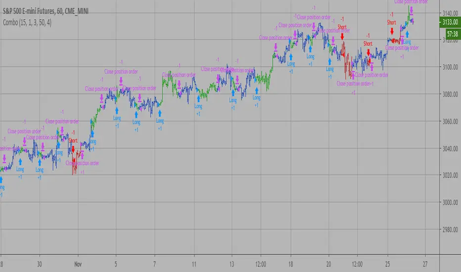
Combo Backtest 123 Reversal & D_ELI (Ehlers Leading Indicator) This is combo strategies for get a cumulative signal.
First strategy
This System was created from the Book "How I Tripled My Money In The
Futures Market" by Ulf Jensen, Page 183. This is reverse type of strategies.
The strategy buys at market, if close price is higher than the previous close
during 2 days and the meaning of 9-days Stochastic Slow Oscillator is lower than 50.
The strategy sells at market, if close price is lower than the previous close price
during 2 days and the meaning of 9-days Stochastic Fast Oscillator is higher than 50.
Second strategy
This Indicator plots a single
Daily DSP (Detrended Synthetic Price) and a Daily ELI (Ehlers Leading
Indicator) using intraday data.
Detrended Synthetic Price is a function that is in phase with the dominant
cycle of real price data. This one is computed by subtracting a 3 pole Butterworth
filter from a 2 Pole Butterworth filter. Ehlers Leading Indicator gives an advanced
indication of a cyclic turning point. It is computed by subtracting the simple
moving average of the detrended synthetic price from the detrended synthetic price.
Buy and Sell signals arise when the ELI indicator crosses over or under the detrended
synthetic price.
See "MESA and Trading Market Cycles" by John Ehlers pages 64 - 70.
WARNING:
- For purpose educate only
- This script to change bars colors.

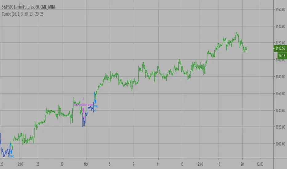
Combo Backtest 123 Reversal & Detrended Synthetic Price V 2 This is combo strategies for get a cumulative signal.
First strategy
This System was created from the Book "How I Tripled My Money In The
Futures Market" by Ulf Jensen, Page 183. This is reverse type of strategies.
The strategy buys at market, if close price is higher than the previous close
during 2 days and the meaning of 9-days Stochastic Slow Oscillator is lower than 50.
The strategy sells at market, if close price is lower than the previous close price
during 2 days and the meaning of 9-days Stochastic Fast Oscillator is higher than 50.
Second strategy
Detrended Synthetic Price is a function that is in phase with the
dominant cycle of real price data. This DSP is computed by subtracting
a half-cycle exponential moving average (EMA) from the quarter cycle
exponential moving average.
See "MESA and Trading Market Cycles" by John Ehlers pages 64 - 70.
WARNING:
- For purpose educate only
- This script to change bars colors.
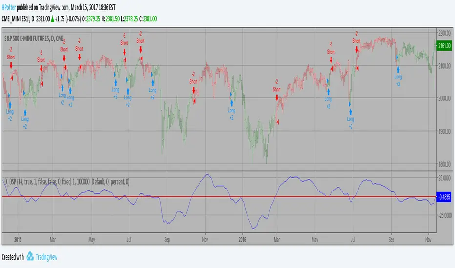
Combo Backtest 123 Reversal & D_DSP (Detrended Synthetic Price) This is combo strategies for get a cumulative signal.
First strategy
This System was created from the Book "How I Tripled My Money In The
Futures Market" by Ulf Jensen, Page 183. This is reverse type of strategies.
The strategy buys at market, if close price is higher than the previous close
during 2 days and the meaning of 9-days Stochastic Slow Oscillator is lower than 50.
The strategy sells at market, if close price is lower than the previous close price
during 2 days and the meaning of 9-days Stochastic Fast Oscillator is higher than 50.
Second strategy
Detrended Synthetic Price is a function that is in phase with the
dominant cycle of real price data. This DSP is computed by subtracting
a half-cycle exponential moving average (EMA) from the quarter cycle
exponential moving average.
See "MESA and Trading Market Cycles" by John Ehlers pages 64 - 70.
WARNING:
- For purpose educate only
- This script to change bars colors.

Fourier series Model Of The Market█ OVERVIEW
The Fourier Series Model of the Market (FSMM) decomposes price action into harmonic components using bandpass filtering, then reconstructs a composite wave weighted by rolling energy ratios. This approach isolates cyclical market behavior at multiple frequencies, emphasizing dominant cycles for cleaner signal generation. The energy-adaptive weighting is the key differentiator from simple harmonic summation: cycles that dominate current price action contribute more to the output.
Based on Fourier analysis principles applied to financial markets, the indicator extracts harmonics (fundamental, 2nd, 3rd, etc.) using second-order IIR bandpass filters, then weights each harmonic's contribution by its relative energy compared to adjacent harmonics. This energy-adaptive weighting naturally emphasizes the cycles that are most prominent in current market conditions.
█ CONCEPTS
Fourier Decomposition
Fourier analysis represents any periodic signal as a sum of sine waves at different frequencies. In market analysis, price action can be decomposed into a fundamental cycle (the base period) plus harmonics at integer multiples of that frequency (period/2, period/3, etc.). Each harmonic captures oscillations at a specific frequency band, and their sum reconstructs the original cyclical behavior.
Bandpass Filtering
Each harmonic is extracted using a second-order IIR (Infinite Impulse Response) bandpass filter tuned to that harmonic's frequency. The filter isolates price activity within a narrow frequency range while rejecting both higher-frequency noise and lower-frequency trend drift. Before filtering, the source is debiased via 2-bar momentum to remove DC offset, ensuring each bandpass operates around true zero.
Energy-Weighted Reconstruction
Rather than simply summing all harmonics equally, FSMM weights each harmonic by its rolling energy relative to the previous harmonic. The energy score combines the current harmonic value with its rate of change, so it reflects both amplitude and momentum. Higher harmonics that hold comparatively more energy therefore contribute more to the composite wave, while weaker harmonics fade out. This adaptive weighting allows the model to respond to changing market cyclicality.
Quadrature Component (Rate of Change)
The rate of change output represents the 90°-phase-shifted (quadrature) component of the wave. When the wave is at zero and rising, the rate of change is at maximum positive. This provides complementary information about cycle phase and can be used for timing entries relative to cycle position.
█ INTERPRETATION
Wave Output
The composite wave oscillates around zero, representing the sum of all extracted harmonic components weighted by energy:
• Above zero : Net bullish cyclical momentum across harmonics
• Below zero : Net bearish cyclical momentum across harmonics
• Zero crossings : Cycle phase transitions - potential reversal points
• Wave amplitude : Strength of cyclical behavior; larger swings indicate cleaner cycles
Rate of Change
The quadrature component (90° phase-shifted) provides cycle phase information:
• Maximum rate of change : Wave is near zero and accelerating - early cycle phase
• Zero rate of change : Wave is at peak or trough - cycle extremes
• Rate/Wave divergence : When wave makes new highs/lows but rate of change does not confirm (lower momentum), suggests cycle exhaustion or impending phase shift
Combined Analysis
• Wave crossing above zero with positive rate of change: Strong bullish cycle initiation
• Wave crossing below zero with negative rate of change: Strong bearish cycle initiation
• Wave at extreme with rate of change reversing: Potential cycle peak/trough
Threshold Bands
When enabled, threshold bands define statistically significant wave deviations:
• Breach above +threshold : Unusually strong bullish cyclical behavior
• Breach below -threshold : Unusually strong bearish cyclical behavior
• Return inside thresholds : Normalizing behavior, potential mean reversion ahead
Alert Conditions
Four built-in alerts trigger on bar close (no repainting):
• Above +Threshold : Strong bullish cycle behavior
• Below -Threshold : Strong bearish cycle behavior
• Above Zero : Bullish cycle phase shift
• Below Zero : Bearish cycle phase shift
█ SETTINGS & PARAMETER TUNING
Fourier Series Model
• Source : Price series to decompose into harmonic components.
• Period (6-100): Base period for the fundamental harmonic. Higher harmonics divide this period (harmonic 2 = period/2, harmonic 3 = period/3). Match to the dominant market cycle for best results. Default 20.
• Bandwidth (0.05-0.5): Bandpass filter selectivity. Lower values create narrower passbands that isolate harmonics more precisely but may miss slightly off-frequency cycles. Higher values capture broader ranges but reduce harmonic separation. Default 0.1 balances precision and robustness.
• Harmonics (1-20): Number of harmonic components to extract. More harmonics capture finer cyclical detail but increase computation. For most applications, 3-5 harmonics suffice. The fundamental alone (1 harmonic) functions as a simple bandpass filter.
Display Settings
• Wave Outputs : Toggle visibility and color of the composite Fourier wave.
• Rate of Change : Toggle visibility and color of the quadrature component (90° phase-shifted wave).
• Zero Line : Reference line for oscillator neutrality.
Diagnostics - Dynamic Thresholds
Optional significance bands that identify when wave readings indicate strong cyclical behavior:
• Dynamic Threshold : Toggle threshold bands and set colors.
• Threshold Mode : Select calculation method:
- MAD (Median Absolute Deviation) : Robust, outlier-resistant measure using k * MAD where MAD ≈ 0.6745 * stdev.
- Standard Deviation : Volatility-sensitive, calculated as k * stdev of wave over the lookback period.
- Percentile Rank : Fixed probability bands using percentile of |wave| (90% means only 10% of values exceed threshold).
• Period (2-200): Lookback for threshold calculations. Default 50.
• Multiplier (k) : Scaling for MAD/Standard Deviation modes. Default 1.5.
• Percentile (%) (0-100): For Percentile Rank mode only. Default 90%.
Parameter Interactions
• Shorter periods respond faster to cycle changes but may capture noise.
• Lower bandwidth + more harmonics = more precise decomposition but requires accurate period setting.
• Higher bandwidth is more forgiving of period mismatches.
• For strongly trending markets, restrict harmonics to 1-2 so the model tracks the dominant cycle with fewer higher-frequency components.
• For ranging/oscillating markets, more harmonics (4-6) capture complex cycles.
█ LIMITATIONS
Inherent Characteristics
• Period dependency : Effectiveness depends on correctly matching the Period parameter to actual market cycles. Use cycle measurement tools (autocorrelation, FFT, dominant cycle indicators) to identify appropriate periods.
• Stationarity assumption : The indicator assumes cycle frequencies remain relatively stable within the lookback window. Rapidly shifting dominant cycles (regime transitions) may produce inconsistent results until the buffer adapts.
• Filter lag : Despite bandpass design, some lag remains inherent to causal filtering. Higher harmonics have less lag but more noise sensitivity.
• Energy weighting artifacts : During regime changes when harmonic energy ratios shift rapidly, weighting may produce transient anomalies.
Market Conditions to Avoid
• Strong trending markets : Pure trends with no cyclicality produce weak, meandering signals. The indicator assumes cyclical market behavior.
• News events/gaps : Large discontinuities disrupt filter continuity. Requires 1-2 full periods to stabilize.
• Period mismatch : If the Period parameter doesn't match actual market cycles, harmonic extraction produces noise rather than signal.
Parameter Selection Pitfalls
• Too many harmonics : Beyond 5-6 harmonics, additional components often capture noise rather than meaningful cycles.
• Bandwidth too narrow : Very low bandwidth (< 0.05) requires extremely precise period matching; slight mismatches cause signal loss.
• Over-optimization : Perfect historical parameter fits typically fail forward. Use robust defaults across multiple instruments.
█ NOTES
Credits
This indicator applies Fourier analysis principles to financial market data, building on the extensive work of Dr. John F. Ehlers in applying digital signal processing to trading. The bandpass filter implementation and harmonic decomposition approach draw from DSP fundamentals as presented in Ehlers' publications.
For those interested in the underlying mathematics and DSP concepts:
• Ehlers, J.F. (2001). Rocket Science for Traders: Digital Signal Processing Applications . John Wiley & Sons.
• Ehlers, J.F. (2013). Cycle Analytics for Traders . John Wiley & Sons.
• Various TASC articles by John Ehlers on bandpass filters, cycle analysis, and harmonic decomposition.
by ♚@e2e4

Voss Predictive Filter█ OVERVIEW
The Voss Predictive Filter (VPF) is a negative group delay (NGD) filter that anticipates cyclical price movement through phase compensation. The VPF isolates band-limited cyclical components via a bandpass filter, then applies negative group delay to shift the signal's phase forward, causing the output to lead the input by a fraction of the cycle period.
Based on Dr. John F. Ehlers' "Voss Predictive Filter" article in Technical Analysis of Stocks & Commodities (TASC) magazine, the VPF displays a predictive oscillator with optional dynamic threshold bands for identifying significant cycle behavior. The indicator is timeframe-agnostic - the mathematics work identically from tick charts to monthly bars, though shorter timeframes require more careful parameter selection due to noise.
█ CONCEPTS
Bandpass Filtering
A bandpass filter isolates price activity within a specific frequency range, removing both high-frequency noise and low-frequency trend drift. The VPF uses a second-order IIR (Infinite Impulse Response) bandpass filter characterized by the center frequency (the Bandpass Period input) and bandwidth. The center frequency determines which cycle period the filter emphasizes, while bandwidth controls the damping coefficient - how tightly the filter focuses around that frequency. Before filtering, the source is debiased via 2-bar momentum to remove DC offset, ensuring the filter operates around a true zero centerline.
Negative Group Delay Filtering
The predictive capability stems from negative group delay (NGD) - a filter characteristic where output appears to "lead" the input. Most causal filters introduce lag (positive group delay), but by combining the bandpass filter output with appropriately weighted past values, the VPF achieves negative group delay characteristics.
This is a universal NGD filter application for band-limited signals: the bandpass filter isolates the cyclical component of interest, then the NGD stage advances the phase within this limited frequency range to create an anticipatory output. This isn't statistical forecasting; it's phase compensation that shifts the signal's timing forward, causing peaks and troughs to appear before they occur in the bandpass output.
Negative Group Delay Stage
The NGD stage combines the current bandpass output with weighted historical values to produce an output that leads the input. By subtracting a weighted average of past deviations from a scaled version of the current filter value, the algorithm advances the signal's phase: peaks and zero-crossings in the voss output appear before the corresponding events in the bandpass filter.
The prediction order (`3 * Prediction Multiplier`) controls how many past values contribute to the phase advance. Higher orders provide smoother output but reduce the leading effect; lower orders maximize anticipation at the cost of stability.
█ INTERPRETATION
Zero-Line Crossovers
Crossings above zero suggest bullish momentum in the filtered cycle; below zero suggests bearish momentum. Crossings from near-zero regions are most reliable, as extreme excursions need time to return to equilibrium.
Threshold Bands
Threshold bands define "significant" deviation. Breaches indicate unusually strong behavior and can serve as:
• Trend confirmation when aligned with price direction
• Overbought/oversold warnings at extremes
• Trade entry filters (requiring threshold breach in the intended direction)
Threshold Mode affects sensitivity: MAD (outlier-resistant), Standard Deviation (volatility-sensitive), Percentile Rank (fixed probability bands).
Alert Conditions
Four built-in alerts trigger on bar close (no repainting): Above +Threshold (strong bullish cycle), Below -Threshold (strong bearish cycle), Above Zero (bullish phase shift), Below Zero (bearish phase shift).
█ SETTINGS & PARAMETER TUNING
Voss Predictive Filter
• Source : Price series to filter.
• Bandpass Period (1-100): Primary tuning parameter determining which cycle length the filter emphasizes. Short periods (8-15) are more responsive but noisier; medium periods (16-30) balance responsiveness and smoothness; long periods (31-100) focus on longer cycles with more smoothing.
• Bandwidth (0.01-0.45): Controls filter selectivity. Narrow bandwidths (0.01-0.15) isolate specific cycle periods precisely; medium (0.16-0.30) tolerate cycle irregularity; wide (0.31-0.45) capture broader cycle ranges. Shorter periods pair well with narrower bandwidths.
• Prediction Multiplier (2-10): Controls how many past values contribute to the phase advance. Higher values provide smoother output but reduce the leading effect; lower values maximize anticipation at the cost of stability.
Display Settings
Control visibility and colors of the Voss output, bandpass filter, and zero reference lines.
Diagnostics - Dynamic Thresholds
Three methods identify significant signal deviation:
• MAD (Median Absolute Deviation) : Robust, outlier-resistant measure using `k * MAD` where `MAD ≈ 0.6745 * stdev`.
• Standard Deviation : Volatility-sensitive, calculated as `k * stdev` of Voss over the lookback period.
• Percentile Rank : Fixed probability bands using the percentile of |Voss| (e.g., 90% means only 10% of values exceed threshold).
Settings:
• Dynamic Threshold : Toggle threshold bands and set colors.
• Threshold Mode : Select MAD, Standard Deviation, or Percentile Rank.
• Period (2-200): Lookback for threshold calculations. Default 50.
• Multiplier (k) : Scaling for MAD/Standard Deviation modes. Default 1.5.
• Percentile (%) (0-100): For Percentile Rank mode only. Default 90%.
█ LIMITATIONS
Inherent Characteristics
• Residual lag : Despite negative group delay design, some lag remains relative to price action.
• Cyclical markets required : Performs best on instruments with clear cyclical components. Strongly trending markets with little cyclicality produce less useful signals.
• Signal interpretation : Absolute Voss values are instrument-specific. Always interpret relative to adaptive threshold bands, not fixed levels.
Market Conditions to Avoid
• Sudden news events/gaps : Major discontinuities disrupt cycle continuity, causing erratic signals. Requires 1-2 full cycle periods to re-stabilize.
• Low volume/illiquid markets : Sporadic trading produces false cycles from liquidity artifacts. Use only on actively traded instruments during liquid hours.
• Regime changes : During cyclical ↔ trending transitions, watch for persistent extremes without mean reversion, increasing price/indicator divergence, or unresolved threshold breaches.
Parameter Selection Pitfalls
• Mismatched period : If Bandpass Period doesn't match actual market cycles, the filter produces weak signals. Use cycle measurement tools (FFT, autocorrelation, Dominant Cycle) to identify appropriate periods first.
• Overoptimization : Perfect historical fits typically fail forward. Choose robust parameters that work across multiple instruments and timeframes.
█ NOTES
Credits
This indicator is based on concepts from Dr. John F. Ehlers' work on predictive filters and bandpass techniques for technical analysis. Dr. Ehlers has published extensively on applying digital signal processing methods to financial markets in Technical Analysis of Stocks & Commodities (TASC) magazine. His articles on bandpass filters and predictive techniques, particularly the Voss Predictive Filter concept, provided the theoretical foundation for this implementation.
For those interested in the underlying mathematics and DSP concepts:
• Ehlers, J.F. (2001). Rocket Science for Traders: Digital Signal Processing Applications . John Wiley & Sons.
• Various TASC articles by John Ehlers on bandpass filters, cycle analysis, and predictive filtering techniques.
• Ehlers, J.F. "Voss Predictive Filter" - Technical Analysis of Stocks & Commodities magazine.
by ♚@e2e4

D_ELI (Ehlers Leading Indicator) Strategy This Indicator plots a single
Daily DSP (Detrended Synthetic Price) and a Daily ELI (Ehlers Leading
Indicator) using intraday data.
Detrended Synthetic Price is a function that is in phase with the dominant
cycle of real price data. This one is computed by subtracting a 3 pole Butterworth
filter from a 2 Pole Butterworth filter. Ehlers Leading Indicator gives an advanced
indication of a cyclic turning point. It is computed by subtracting the simple
moving average of the detrended synthetic price from the detrended synthetic price.
Buy and Sell signals arise when the ELI indicator crosses over or under the detrended
synthetic price.
See "MESA and Trading Market Cycles" by John Ehlers pages 64 - 70.

D_DSP (Detrended Synthetic Price) Strategy 2 Backtest Detrended Synthetic Price is a function that is in phase with the
dominant cycle of real price data. This DSP is computed by subtracting
a half-cycle exponential moving average (EMA) from the quarter cycle
exponential moving average.
See "MESA and Trading Market Cycles" by John Ehlers pages 64 - 70.
You can change long to short in the Input Settings
Please, use it only for learning or paper trading. Do not for real trading.

D_DSP (Detrended Synthetic Price) Strategy 2 Detrended Synthetic Price is a function that is in phase with the
dominant cycle of real price data. This DSP is computed by subtracting
a half-cycle exponential moving average (EMA) from the quarter cycle
exponential moving average.
See "MESA and Trading Market Cycles" by John Ehlers pages 64 - 70.

D_DSP (Detrended Synthetic Price) Strategy Backtest Detrended Synthetic Price is a function that is in phase with the
dominant cycle of real price data. This DSP is computed by subtracting
a half-cycle exponential moving average (EMA) from the quarter cycle
exponential moving average.
See "MESA and Trading Market Cycles" by John Ehlers pages 64 - 70.
D_DSP (Detrended Synthetic Price) Strategy Detrended Synthetic Price is a function that is in phase with the
dominant cycle of real price data. This DSP is computed by subtracting
a half-cycle exponential moving average (EMA) from the quarter cycle
exponential moving average.
See "MESA and Trading Market Cycles" by John Ehlers pages 64 - 70.
