Expected Value Monte CarloI created this indicator after noticing that there was no Expected Value indicator here on TradingView.
The EVMC provides statistical Expected Value to what might happen in the future regarding the asset you are analyzing.
It uses 2 quantitative methods:
Historical Backtest to ground your analysis in long-term, factual data.
Monte Carlo Simulation to project a cone of probable future outcomes based on recent market behavior.
This gives you a data-driven edge to quantify risk, and make more informed trading decisions.
The indicator includes:
Dual analysis: Combines historical probability with forward-looking simulation.
Quantified projections: Provides the Expected Value ($ and %), Win Rate, and Sharpe Ratio for both methods.
Asset-aware: Automatically adjusts its calculations for Stocks (252 trading days) and Crypto (365 days) for mathematical accuracy.
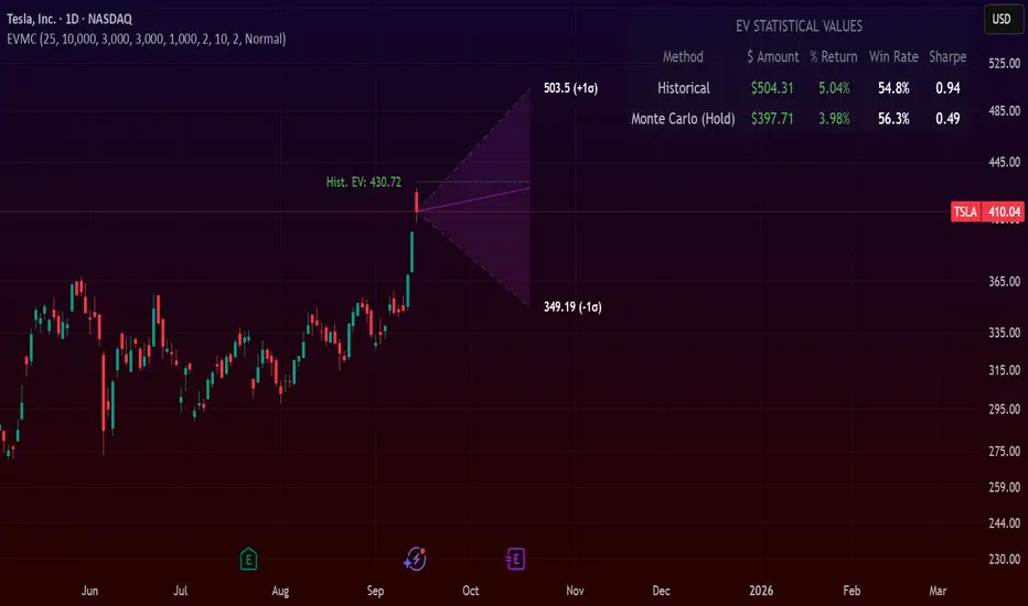
The projection cone shows the mean expected path and the +/- 1 standard deviation range of outcomes.
No repainting
Calculation:
1. Historical Expected Value:
This is a systematic backtest over thousands of bars. It calculates the return Rᵢ for N past trades (buy-and-hold). The Historical EV is the simple average of these returns, giving a baseline performance measure.
Historical EV % = (Σ Rᵢ) / N
2. Monte Carlo Projection:
This projection uses the Geometric Brownian Motion (GBM) model to simulate thousands of future price paths based on the market's recent behavior.
It first measures the drift (μ), or recent trend, and volatility (σ), or recent risk, from the Projection Lookback period. It then projects a final return for each simulation using the core GBM formula:
Projected Return = exp( (μ - σ²/2)T + σ√T * Z ) - 1
(Where T is the time horizon and Z is a random variable for the simulation.)
The purple line on the chart is the average of all simulated outcomes (the Monte Carlo EV). The cone represents one standard deviation of those outcomes.
The dashed lines represent one standard deviation (+/- 1σ) from the average, forming a cone of probable outcomes. Roughly 68% of the simulated paths ended within this cone.
This projection answers the question: "If the recent trend and volatility continue, where is the price most likely to go?"
Here's how to read the indicator
Expected Value ($/%): Is my average trade profitable?
Win Rate: How often can I expect to be right?
Sharpe Ratio: Am I being adequately compensated for the risk I'm taking?
User Guide
Max trade duration (bars): This is your analysis timeframe. Are you interested in the probable outcome over the next month (21 bars), quarter (63 bars), or year (252 bars)?
Position size ($): Set this to your typical trade size to see the Expected Value in real dollar terms.
Projection lookback (bars): This is the most important input for the Monte Carlo model. A short lookback (e.g., 50) makes the projection highly sensitive to recent momentum. Use this to identify potential recency bias. A long lookback (e.g., 252) provides a more stable, long-term projection of trend and volatility.
Historical Lookback (bars): For the historical backtest, more data is always better. Use the maximum that your TradingView plan allows for the most statistically significant results.
Use TP/SL for Historical EV: Check this box to see how the historical performance would have changed if you had used a simple Take Profit and Stop Loss, rather than just holding for the full duration.
I hope you find this indicator useful and please let me know if you have any suggestions. 😊
Expectedvalue
Stop Loss vs Take Profit Probability and EVThis stop loss and take profit calculator uses a Monte Carlo simulation to calculate the probability of hitting your Stop Loss or Take Profit levels across different time horizons (expressed in bars).
It provides data-driven insights to optimize your risk management and position sizing by showing Expected Value for each scenario.
As a quant, I love using statistical data to help my decisions and get better EV from my trades.
🔬 How It's Calculated
Monte Carlo Simulation: Runs 1,000-10,000 price simulations using a random walk model
Volatility Analysis: Combines ATR-based and Historical Volatility for accurate price movement modeling
Expected Value: Calculates profit/loss expectation using formula: (TP_Probability × Reward) - (SL_Probability × Risk)
Time Horizons: Tests multiple timeframes (1, 5, 10, 20, 50 bars) to find optimal holding periods
Risk/Reward Ratios: Automatically calculates and displays R:R ratios for quick assessment
💡 Use Cases
Position Sizing - Determine optimal risk per trade based on Expected Value
Time Horizon Optimization - Find the best holding period for your strategy
Stop Loss Placement - Validate SL levels using probability analysis
Take Profit Optimization - Set TP levels with statistical backing
Strategy Backtesting - Compare different R:R setups before entering trades
Risk Management - Avoid trades with negative Expected Value
Swing vs Day Trading - Choose timeframes with highest success probability
🎯 How to Use
Setup Trade: Enter your entry price, stop loss, and take profit levels
You can add or remove time horizons denominated in bars. Say you are looking at 1h candles, adding a 24-bar time horizon means you are looking into 24 hours
Choose Direction: Select Long or Short position
Review Table
Analyze Expected Value: Focus on positive EV scenarios (green background)
Optimize Timing: Select time horizons with best risk/reward profile
Adjust Parameters: Modify volatility calculation method and simulation count if needed
Examples
Here's how you can read the tables.
Example 1:
In this chart, we are analyzing the TP and SL probabilities as well as the EV (expected value) for a stock. I want to check what the likelihood is that my SL and TP get triggered over the next 5 days. The stock market is open for 6.5 hours per day, which is 13 bars in this 30-minute bar chart. 26 bars is 2 days, 39 bars is 3 days and so on.
Although this trade is more likely to trigger my SL than my TP, in some of the time horizons we have a positive expected value because of the risk/reward of our trade (i.e. distance of the SL and TP from the price) and the probability of hitting SL and TP.
Example 2:
In this example, we have applied the indicator to gold. Because the TP is much closer to the price, the probability of hitting the TP is much higher.
We can also observe that the expected Value in the shorter time frames is better than in the longer ones. This can give us some clues to set up our trade. If we know that the EV is positive, we can allocate more to that specific trade.
Enjoy, and please let me know your feedback! 😊🥂
