Vega Convexity Regime Filter [Institutional Lite]STOP TRADING THE NOISE.
90% of retail trading losses occur during "Chop"—sideways markets where standard trend-following bots bleed capital through slippage and fees. Institutional desks know that the secret to high returns isn't just winning trades; it's knowing when to sit in cash.
The Vega V6 Regime Filter is the "Gatekeeper" layer of our proprietary Hierarchical Machine Learning engine (developed by a 25-year TradFi Risk Quant). It calculates a composite volatility score to answer one simple question: Is this asset tradeable right now?
THE VISUAL LOGIC
This indicator visually filters market conditions into two distinct Regimes based on our institutional backtests:
🌫️ GREY BARS (Noise / Chop)
The State: Volatility is compressing. The trend is undefined or weak.
The Trap: This is where MACD/RSI give false signals.
Institutional Action: Sit in Cash. Preserve Capital. Wait.
🟢 🔴 COLORED BARS (Impulse)
The State: Volatility is expanding. Momentum is statistically significant.
The Opportunity: A "Fat-Tail" move is likely beginning.
Institutional Action: Deploy Risk. Look for entries.
HOW IT WORKS (The Math)
Unlike simple moving average crossovers, the Vega Gatekeeper analyzes 4 distinct market dimensions simultaneously to generate a Tradeability Score (0-10) :
Trend Strength (ADX): Is there a vector?
Momentum (RSI/MACD): Is the move accelerating?
Volatility (Bollinger Bands): Is the range expanding?
Volume Flow: Is there institutional participation?
The Rule: If the composite score is < 4 , the market is Noise. The bars turn Grey. You do nothing.
BEST PRACTICES
For Swing Trading (Daily): Use Medium sensitivity. Only look for entries when the background turns Green/Red.
For Day Trading (4H/1H): Use Low sensitivity (more conservative). Use the Grey zones to tighten stops or exit positions.
THE PHILOSOPHY: "CASH IS A POSITION"
Most traders feel the need to be in a trade 24/7. The Vega V6 Engine (the system this tool is based on) achieved a +3,849% backtested return (18 months) largely by sitting in cash during chop. This tool visualizes that discipline.
🔒 WANT THE DIRECTIONAL SIGNALS?
This Lite version provides the Regime (When to trade).
To get the specific Entry Signals , Intraday Stop-Losses , and Probability Matrix (Stage 2 of our model), you need the Vega V6 Convexity Engine .
The Pro Version includes:
🚀 Specific Direction: Classification of "Explosion," "Rally," or "Crash."
🛡️ Dynamic Risk: Plots the exact Stop Loss levels used in our institutional backtests.
🌊 Macro Data: Integration of M2 Liquidity flow alerts.
👉 ACCESS INSTRUCTIONS:
Links to the Pro System , our Live Dashboard , and the 18-Month Performance Audit can be found in the Author Profile below or in the script settings.
Disclaimer: This tool is for educational purposes only. Past performance is not indicative of future results. Trading cryptocurrencies involves significant risk.
Filter

Filtered TEMA CrossoverFiltered Dual TEMA Crossover
This indicator is a trend-following tool based on the classic Dual Triple Exponential Moving Average (TEMA) Crossover strategy, enhanced with two robust filters: the Chop Index and the Average Directional Index (ADX).
The TEMA is known for its low lag and high responsiveness, making the crossover an effective signal for trend reversals. However, trading TEMA crossovers during sideways, choppy markets often leads to false signals. This is where the filters come in.
Key Features
▪️Dual TEMA Crossover: Plots two customizable TEMA lines (Fast and Slow) for clear visualization of the primary trend direction.
▪️Intelligent Signal Filtering: Buy and Sell signals are generated only when the market confirms it is in a trending state, thanks to two integrated filters:
➖Chop Index Filter: Blocks signals when the market is detected as sideways or consolidating (Chop Index reading above a user-defined threshold).
➖ADX Filter: Ensures signals are only taken when the trend strength is sufficient (ADX reading above a user-defined minimum threshold).
▪️Customizable Signals: Full control over the signal shapes (Arrows, Triangles, etc.), colors, text, and size.
How to Use It
Use the Filtered Dual TEMA Crossover to enter positions on trend continuation or reversal while dramatically reducing exposure to low-quality, whipsawing signals common in non-trending environments.
Before the filters:
After the filters:
Minimize Noise. Maximize Clarity. Trade the Trend.

Multi-Filter & RSI Overheat Analyzer (Invite Only)🚀 Multi-Filter & RSI Overheat Analyzer (Invite Only)
The Trend-RSI Pro is an advanced, multi-layered analysis tool designed for invite-only subscribers. Its primary function is to provide an instant, high-conviction visual filter of current market conditions by combining three essential technical analyses: EMA trend direction, ADX trend strength, and RSI overbought/oversold momentum.
💡 Key Features and Analysis Logic
This indicator simplifies complex market structure analysis by using a dynamic Background Color filter. The color instantly tells the user the dominant market state, eliminating the need to manually check multiple windows.
The background turns Teal when the Exponential Moving Averages (EMA) are in a strong Bullish Alignment (Short > Medium > Long) and the ADX value exceeds the user-defined Strength Threshold (default 25.0), confirming a Strong Uptrend. Conversely, the background turns Red when the EMAs are in a strong Bearish Alignment (Short < Medium < Long) and the ADX confirms a Strong Downtrend. Any other combination of EMA alignment or a weak ADX reading results in a Gray background, which alerts the user to a Ranging, Weak, or Transitional Market where caution is advised.
To complement the trend analysis, the indicator features RSI Overheat Alert Icons to preemptively analyze potential trend exhaustion. When the Relative Strength Index (RSI) enters the Overbought zone (default >= 70.0), a Red Triangle Down appears above the price bar, warning of potential selling pressure. Conversely, when the RSI enters the Oversold zone (default <= 30.0), a Green Triangle Up appears below the price bar, suggesting potential buying interest.
For users who wish to confirm the underlying components, the indicator also plots the three EMA Lines (Short, Medium, Long) directly on the chart, and the raw ADX Value is plotted in a separate pane, allowing for detailed tracking of strength changes over time. All key parameters, including EMA periods, ADX thresholds, and RSI limits, are fully customizable in the settings.
⚠️ Disclaimer and Usage Guideline
This tool is strictly an analytical aid and not a trading signal or financial advice. Users should utilize the Background Color as their primary context filter, only seeking trades aligned with the indicated strong trend color. The RSI alerts serve as timely warnings for potential short-term reversals within a larger trend. Trading carries substantial risk, and this indicator must always be combined with the user's independent analysis and robust risk management strategies.

Hurst Flow • @Capital.comDescription
Hurst Flow is a regime-adaptive analytical tool that measures the continuous intention force behind market behavior.
It blends momentum and persistence analysis to quantify how strongly price movement aligns with trend continuation versus mean reversion.
The output is a normalized continuous force line:
Positive values indicate increasing long-side capital exposure — markets showing trend-persistence and momentum alignment.
Negative values reflect strengthening short-side capital exposure — environments favoring mean reversion or fading moves.
Internally, the indicator processes open-price rate-of-change dynamics through adaptive smoothing, persistence estimation, and standardized scaling, producing a stable and comparable signal across time frames and assets.
Use Hurst Flow as a market regime compass — to gauge bias, filter trades, or allocate exposure intensity dynamically.
Input descriptions
TF — Timeframe used to compute the signal. Higher TF = smoother, less whipsaw, but more lag.
ROC length (Open) — Lookback for Open-to-Open rate of change (base momentum horizon).
EMA length — Smoothing for ROC; increases stability at the cost of responsiveness.
Hurst window — Window for Hurst-style persistence estimate; governs regime sensitivity.
Standartizatoin window — Period for standardization; makes values comparable across assets/timeframes.
Scale factor (0..1) — Final gain applied to the standardized signal; use <1 to temper amplitude.
Presets/Backtest
Below is a list of presets that can be used to test indicators. The presets cover various asset classes and time frames, demonstrating versatility and high customizability. To do this, you can use a special strategy Target % Rebalancer Based Strategy on Intention Indicator . The entry signal for the strategy is the output signal of the indicator from the chart, which can be selected from a special drop-down list. A detailed description of the strategy can be found on a special page. The presets presented were created on instruments not included in the sample.
Below are the basic presets for the strategy. Other configuration functions can be used to fine-tune the strategy.
The strategy settings are the same for all of the presets listed. The time interval must be set for both the indicator and the chart.
Strategy fine tuning
Enable Hysteresis + Cooldown : Off
Risk & costs
Enable Max Daily Loss Halt : Off
Commission : 0.1%
============== Pre-Sets for Hurst Flow Indicator =============================
Preset Gold
Chart bar size: 3D
Indicator settings
TF : 3D
ROC : 10
EMA : 22
Hurst : 16
Standardization window length : 8
Scale : 1
====================================================
Preset Crude Oil:USOIL
Chart bar size: 1D
Indicator settings
TF : 1D
ROC : 70
EMA : 6
Hurst : 26
Standardization window length : 16
Scale : 1
Final Weight Cap : 1
====================================================
Preset S&P500 index
Chart bar size: 2D
Indicator settings
TF : 2D
ROC : 26
EMA : 8
Hurst : 33
Standardization window length : 16
Scale : 1
====================================================
Preset MSFT
Chart bar size: 2D
Indicator settings
TF : 2D
ROC : 16
EMA : 50
Hurst : 44
Standardization window length : 32
Scale : 1

ATR Trend + RSI Pullback Strategy [Profit-Focused]This strategy is designed to catch high-probability pullbacks during strong trends using a combination of ATR-based volatility filters, RSI exhaustion levels, and a trend-following entry model.
Strategy Logic
Rather than relying on lagging crossovers, this model waits for RSI to dip into oversold zones (below 40) while price remains above a long-term EMA (default: 200). This setup captures pullbacks in strong uptrends, allowing traders to enter early in a move while controlling risk dynamically.
To avoid entries during low-volatility conditions or sideways price action, it applies a minimum ATR filter. The ATR also defines both the stop-loss and take-profit levels, allowing the model to adapt to changing market conditions.
Exit logic includes:
A take-profit at 3× the ATR distance
A stop-loss at 1.5× the ATR distance
An optional early exit if RSI crosses above 70, signaling overbought conditions
Technical Details
Trend Filter: 200 EMA – must be rising and price must be above it
Entry Signal: RSI dips below 40 during an uptrend
Volatility Filter: ATR must be above a user-defined minimum threshold
Stop-Loss: 1.5× ATR below entry price
Take-Profit: 3.0× ATR above entry price
Exit on Overbought: RSI > 70 (optional early exit)
Backtest Settings
Initial Capital: $10,000
Position Sizing: 5% of equity per trade
Slippage: 1 tick
Commission: 0.075% per trade
Trade Direction: Long only
Timeframes Tested: 15m, 1H, and 30m on trending assets like BTCUSD, NAS100, ETHUSD
This model is tuned for positive P&L across trending environments and volatile markets.
Educational Use Only
This strategy is for educational purposes only and should not be considered financial advice. Past performance does not guarantee future results. Always validate performance on multiple markets and timeframes before using it in live trading.

TASC 2025.12 The One Euro Filter█ OVERVIEW
This script implements the One Euro filter, developed by Georges Casiez, Nicolas Roussel, and Daniel Vogel, and adapted by John F. Ehlers in his article "Low-Latency Smoothing" from the December 2025 edition of the TASC Traders' Tips . The original creators gave the filter its name to suggest that it is cheap and efficient, like something one might purchase for a single Euro.
█ CONCEPTS
The One Euro filter is an EMA-based low-pass filter that adapts its smoothing factor (alpha) based on the absolute values of smoothed rates of change in the source series. It was designed to filter noisy, high-frequency signals in real time with low latency. Ehlers simplifies the filter for market analysis by calculating alpha in terms of bar periods rather than time and frequency, because periods are naturally intuitive for a discrete financial time series.
In his article, Ehlers demonstrates how traders can apply the adaptive One Euro filter to a price series for simple low-latency smoothing. Additionally, he explains that traders can use the filter as a smoothed oscillator by applying it to a high-pass filter. In essence, similar to other low-pass filters, traders can apply the One Euro filter to any custom source to derive a smoother signal with reduced noise and low lag.
This script applies the One Euro filter to a specified source series, and it applies the filter to a two-pole high-pass filter or other oscillator, depending on the selected "Osc type" option. By default, it displays the filtered source series on the main chart pane, and it shows the oscillator and its filtered series in a separate pane.
█ INPUTS
Source: The source series for the first filter and the selected oscillator.
Min period: The minimum cutoff period for the smoothing calculation.
Beta: Controls the responsiveness of the filter. The filter adds the product of this value and the smoothed source change to the minimum period to determine the filter's smoothing factor. Larger values cause more significant changes in the maximum cutoff period, resulting in a smoother response.
Osc type: The type of oscillator to calculate for the pane display. By default, the indicator calculates a high-pass filter. If the selected type is "None", the indicator displays the "Source" series and its filtered result in a separate pane rather than showing the filter on the main chart. With this setting, users can pass plotted values from another indicator and view the filtered result in the pane.
Period: The length for the selected oscillator's calculation.

ADX Trend Strength Filter + TRAMA [DotGain]Summary
Are you tired of trading trend signals, only to get stopped out in volatile, sideways chop?
The ADX Trend Strength Filter (ADX TSF) is designed to solve this exact problem. It is a comprehensive trend-following system that only generates signals when a trend not only has the right direction and momentum, but also sufficient strength.
This indicator filters out weak or indecisive market phases (the "chop") and will only color the bars Green or Red when all conditions for a strong, confirmed trend are met.
⚙️ Core Components and Logic
The ADX TSF relies on a triple-filter logic to generate a clear trade signal:
Trend Filter (TRAMA): A TRAMA (Trending Adaptive Moving Average) is used as the main trendline. This adaptive average automatically adjusts to market volatility, acting as a dynamic support/resistance level.
Price > TRAMA = Bullish
Price < TRAMA = Bearish
Momentum Filter (RSI Crossover): Momentum is measured by a crossover of two moving averages of the RSI (a fast EMA and a slow SMA). This confirms whether the momentum is pointing in the same direction as the trend.
Strength Filter (ADX): This is the most important filter. A signal is only considered valid if the ADX (Average Directional Index) is above a defined threshold (Default: 30). This ensures the trend has sufficient strength.
🚦 How to Read the Indicator
The indicator has three states, displayed directly as bar colors on your chart:
🟩 GREEN BARS (Strong Uptrend) All three conditions are met:
Price is above the TRAMA.
RSI momentum is bullish (Fast MA > Slow MA).
ADX is above 30 (Strong trend is present).
🟥 RED BARS (Strong Downtrend) All three conditions are met:
Price is below the TRAMA.
RSI momentum is bearish (Fast MA < Slow MA).
ADX is above 30 (Strong trend is present).
🟧 ORANGE BARS (Neutral / Caution) This state appears if any of the following conditions are true:
Weak Trend: The ADX is below 30. The market is in consolidation or a sideways phase. (This is the primary filter!)
Indecision: The price is caught in the "Neutral Zone" between the TRAMA and the 200 SMA.
Visual Elements
Bar Colors: (Green/Red/Orange) Show the current trend status.
TRAMA (Orange Line): Your primary adaptive trendline.
200 SMA (White Line): Serves as a reference for the long-term trend.
Orange Background (Fill): Fills the area between the TRAMA and SMA to visually highlight the "Neutral Zone."
Key Benefit
The goal of the ADX TSF is to keep traders out of weak, unpredictable markets and help them participate only in strong, momentum-confirmed trends.
Have fun :)
Disclaimer
This "Buy The F*cking Dip" (BTFD) indicator is provided for informational and educational purposes only. It does not, and should not be construed as, financial, investment, or trading advice.
The signals generated by this tool (both "Buy" and "Sell") are the result of a specific set of algorithmic conditions. They are not a direct recommendation to buy or sell any asset. All trading and investing in financial markets involves substantial risk of loss. You can lose all of your invested capital.
Past performance is not indicative of future results. The signals generated may produce false or losing trades. The creator (© DotGain) assumes no liability for any financial losses or damages you may incur as a result of using this indicator.
You are solely responsible for your own trading and investment decisions. Always conduct your own research (DYOR) and consider your personal risk tolerance before making any trades.

ATR Support LineOverview
ATR Support Line is a higher-timeframe-aware overlay that builds a single dynamic support line by anchoring a smoothed price baseline and offsetting it with an Average True Range (ATR) multiple. It is designed to track constructive trends while adapting to current volatility. The tool can render using higher-timeframe (HTF) data with optional closed-bar confirmation to avoid repainting, or live interpolation for more responsive visuals.
Core logic (concepts, not implementation)
• Compute an anchor from price using a selectable moving-average family (SMA / EMA / ZLEMA).
• Measure volatility using ATR and apply a configurable multiplier.
• Form the support line by offsetting the anchor downward by the ATR multiple.
• Timeframe handling: either use the chart timeframe or request an explicit HTF for calculation.
• Rendering modes:
– Closed-bar mode : interpolate inside the previous HTF bar for non-repainting behavior.
– Live mode : interpolate inside the current HTF bar for more timely responsiveness (can visually “breathe” intrabar).
Inputs
• Anchor smoothing: MA type (SMA / EMA / ZLEMA) and anchor length.
• Volatility: ATR length and multiplier.
• Timeframe: optional calculation timeframe (HTF) distinct from the chart timeframe.
• Confirmation: toggle to use closed HTF values (non-repainting) vs. live interpolation.
How to read it
• Price holding above the ATR Support Line indicates constructive conditions; orderly pullbacks toward the line can be normal trend behavior.
• Persistent closes above the line indicate strength; reactions into the line often resolve higher in constructive regimes.
• Persistent closes below the line warn of deterioration; consider reducing risk until price reclaims the level.
• On HTF rendering with closed-bar confirmation, use closes on that HTF for signal confirmation.
• In live mode, treat intrabar pierces as potential noise until confirmed by the close.
Practical use cases
• Trend context: define a trailing “line in the sand” for long-bias frameworks.
• Risk framing: size down or tighten exposure when price loses the support line.
• Confluence: combine with structure (HH/HL vs. LH/LL), volume, or market-wide risk gauges.
• Multi-TF workflow: calculate on HTF for bias, execute on lower TFs for entries/exits.
Best practices
• Align confirmations with the timeframe used for calculation (especially in closed-bar mode).
• Pair with clear invalidation rules (e.g., daily/weekly closes below the line).
• Start with conservative multipliers on noisier assets; adjust ATR length/multiplier to match instrument volatility.
Technical notes
• Non-repainting option : closed-bar HTF mode finalizes values on HTF close; lower-TF plotting uses interpolation only for continuity (no look-ahead).
• Live option : interpolates within the current HTF bar for responsiveness; expect intrabar breathing.
• Works on any time-based chart; results are most interpretable on liquid instruments.
Who it is for
• Traders who want a single, disciplined, volatility-adjusted support line with HTF awareness.
• Systematic users who prefer clear, reproducible rules for trend context and risk boundaries.
Limitations & disclosures
• Closed-source; for educational and analytical use only.
• Not financial advice. Markets involve risk; past performance does not guarantee future results.
Release notes
• Added selectable anchor MA (SMA / EMA / ZLEMA) and explicit HTF calculation with two rendering modes (closed-bar non-repainting vs. live).
• Interpolation refined for smooth visuals while respecting HTF closes in confirmation mode.
Originality & why closed-source
This is not a reimplementation of public open-source scripts. The integration of anchor smoothing choices, volatility offset, HTF calculation, and dual rendering modes (closed-bar non-repainting vs. live interpolation) is designed to maintain trend fidelity with practical control over responsiveness. The interaction of these components is proprietary and the source is closed to protect the implementation.
Integration, not a mashup
ATR Support Line is a single, self-contained framework. It does not merely merge indicators; its components are purpose-built to produce one coherent, volatility-aware, single-line support with a clear reading protocol (hold above = constructive; loss = caution).
Indicator, not a strategy
This publication is an indicator overlay, not a trading strategy. It includes no backtests, position logic, performance claims, or risk assumptions. Use it as analytical context within your own risk management.
Comparison to common tools
Compared to static moving-average baselines or classic volatility bands, ATR Support Line emphasizes (1) a single actionable support level, (2) explicit volatility adjustment via ATR, and (3) HTF-aware rendering with an optional non-repainting confirmation mode.

Kalman Adaptive Score Overlay [BackQuant]Kalman Adaptive Score Overlay
A powerful indicator that uses adaptive scoring to assess market conditions and trends, utilizing advanced filtering techniques to smooth price data, enhance trend-following precision, and predict future price movements based on past data. It is ideal for traders who need a dynamic and responsive trend analysis tool that adjusts to market fluctuations.
What is Adaptive Scoring?
Adaptive scoring is a technique that adjusts the weight or importance of certain price movements over time based on an ongoing assessment of market behavior. This indicator uses dynamic scoring to assess the strength and direction of price movements, providing insight into whether a trend is likely to continue or reverse. The score is recalculated continuously to reflect the most up-to-date market conditions, offering a responsive approach to trend-following.
How It Works
The core of this indicator is built on advanced filtering methods that smooth price data, adjusting the response to recent price changes. The filtering mechanism incorporates a Kalman filter to reduce noise and improve the accuracy of price signals. Combined with adaptive scoring, this creates a robust framework that automatically adjusts to both short-term fluctuations and long-term trends.
The indicator also uses a dynamic trend-following component that updates its analysis based on the direction of the market, with the option to visualize it through colored candles. When a strong trend is identified, the candles are painted to reflect the prevailing trend, helping traders quickly identify whether the market is in a bullish or bearish state.
Why Adaptive Scoring Is Important
Dynamic Response: Adaptive scoring allows the indicator to respond to changing market conditions. By adjusting its sensitivity to price fluctuations, it ensures that trends are captured accurately, without being overly influenced by short-term noise.
Trend Precision: By combining Kalman filtering with adaptive scoring, the indicator offers a precise and smooth trend-following mechanism. It helps traders stay aligned with the market direction and avoid false signals.
Versatility: The indicator works across multiple timeframes, making it adaptable to different trading strategies, from scalping to long-term trend-following.
Confidence in Market Moves: The adaptive scoring component provides traders with confidence in the strength of the trend, helping them determine when to enter or exit positions with greater certainty.
How Traders Use It
Trend-Following Strategy: Traders can use this indicator to confirm trends and refine their entries and exits. The colored candles and adaptive scoring offer a visual cue of trend strength and direction, making it easier to follow the prevailing market movement.
Multi-Timeframe Analysis: The script supports multi-timeframe analysis, allowing traders to analyze trends and scores across different timeframes (e.g., 1m, 5m, 15m, 30m, 1h, 4h, 12h). This is useful for traders who want to confirm trends on both short and long-term charts before making a trade.
Refining Entry Points: By utilizing the adaptive scoring, traders can identify potential entry points where the score indicates a high probability of trend continuation. Higher scores signal stronger trends, guiding decision-making.
Managing Risk: Traders can use the adaptive scoring system to assess trend stability and adjust their risk management strategies accordingly. For example, higher confidence in the trend allows for larger positions, while lower confidence may require smaller, more cautious trades.
Key Features and Benefits
Kalman Filter for Noise Reduction: The Kalman filter helps to smooth out market noise and allows for a clearer understanding of the underlying price movements. This is particularly useful in volatile markets where short-term fluctuations can cloud trend analysis.
Adaptive Scoring for Flexibility: Adaptive scoring ensures that the indicator remains responsive to changing market conditions. It automatically adjusts to the strength of price movements, enabling better detection of trends and reversals.
Visual Trend Signals: The indicator provides visual signals through candle coloring, making it easier to identify whether the market is in a bullish, neutral, or bearish phase.
Multi-Timeframe Display: The indicator’s multi-timeframe feature allows traders to see the trend and adaptive score on different timeframes simultaneously, providing a comprehensive view of the market.
Customizable Settings: Traders can customize the indicator’s settings, such as the filter parameters, scoring thresholds, and visualization options, tailoring it to their specific trading style and strategy.
Why This is Important for Traders
Improved Decision Making: The adaptive nature of the scoring system allows traders to make more informed decisions based on real-time market data, without being influenced by past volatility.
Market Clarity: By smoothing out price movements and scoring trends adaptively, the indicator provides a clearer picture of market behavior, which is essential for effective trend-following and timing entries and exits.
Increased Confidence in Signals: Adaptive scoring ensures that signals are based on the current market structure, reducing the likelihood of false positives. This boosts traders' confidence when acting on signals.
Conclusion
The Kalman Adaptive Score Overlay offers a dynamic and responsive trend-following tool that integrates Kalman filtering with adaptive scoring. By adjusting to market fluctuations in real time, it allows traders to identify and follow trends with greater precision. Whether you are trading on short or long timeframes, this tool helps you stay aligned with market momentum, ensuring that your entries and exits are based on the most up-to-date and reliable data available.

Kalman VWAP Filter [BackQuant]Kalman VWAP Filter
A precision-engineered price estimator that fuses Kalman filtering with the Volume-Weighted Average Price (VWAP) to create a smooth, adaptive representation of fair value. This hybrid model intelligently balances responsiveness and stability, tracking trend shifts with minimal noise while maintaining a statistically grounded link to volume distribution.
If you would like to see my original Kalman Filter, please find it here:
Concept overview
The Kalman VWAP Filter is built on two core ideas from quantitative finance and control theory:
Kalman filtering — a recursive Bayesian estimator used to infer the true underlying state of a noisy system (in this case, fair price).
VWAP anchoring — a dynamic reference that weights price by traded volume, representing where the majority of transactions have occurred.
By merging these concepts, the filter produces a line that behaves like a "smart moving average": smooth when noise is high, fast when markets trend, and self-adjusting based on both market structure and user-defined noise parameters.
How it works
Measurement blend : Combines the chosen Price Source (e.g., close or hlc3) with either a Session VWAP or a Rolling VWAP baseline. The VWAP Weight input controls how much the filter trusts traded volume versus price movement.
Kalman recursion : Each bar updates an internal "state estimate" using the Kalman gain, which determines how much to trust new observations vs. the prior state.
Noise parameters :
Process Noise controls agility — higher values make the filter more responsive but also more volatile.
Measurement Noise controls smoothness — higher values make it steadier but slower to adapt.
Filter order (N) : Defines how many parallel state estimates are used. Larger orders yield smoother output by layering multiple one-dimensional Kalman passes.
Final output : A refined price trajectory that captures VWAP-adjusted fair value while dynamically adjusting to real-time volatility and order flow.
Why this matters
Most smoothing techniques (EMA, SMA, Hull) trade off lag for smoothness. Kalman filtering, however, adaptively rebalances that tradeoff each bar using probabilistic weighting, allowing it to follow market state changes more efficiently. Anchoring it to VWAP integrates microstructure context — capturing where liquidity truly lies rather than only where price moves.
Use cases
Trend tracking : Color-coded candle painting highlights shifts in slope direction, revealing early trend transitions.
Fair value mapping : The line represents a continuously updated equilibrium price between raw price action and VWAP flow.
Adaptive moving average replacement : Outperforms static MAs in variable volatility regimes by self-adjusting smoothness.
Execution & reversion logic : When price diverges from the Kalman VWAP, it may indicate short-term imbalance or overextension relative to volume-adjusted fair value.
Cross-signal framework : Use with standard VWAP or other filters to identify convergence or divergence between liquidity-weighted and state-estimated prices.
Parameter guidance
Process Noise : 0.01–0.05 for swing traders, 0.1–0.2 for intraday scalping.
Measurement Noise : 2–5 for normal use, 8+ for very smooth tracking.
VWAP Weight : 0.2–0.4 balances both price and VWAP influence; 1.0 locks output directly to VWAP dynamics.
Filter Order (N) : 3–5 for reactive short-term filters; 8–10 for smoother institutional-style baselines.
Interpretation
When price > Kalman VWAP and slope is positive → bullish pressure; buyers dominate above fair value.
When price < Kalman VWAP and slope is negative → bearish pressure; sellers dominate below fair value.
Convergence of price and Kalman VWAP often signals equilibrium; strong divergence suggests imbalance.
Crosses between Kalman VWAP and the base VWAP can hint at shifts in short-term vs. long-term liquidity control.
Summary
The Kalman VWAP Filter blends statistical estimation with market microstructure awareness, offering a refined alternative to static smoothing indicators. It adapts in real time to volatility and order flow, helping traders visualize balance, transition, and momentum through a lens of probabilistic fair value rather than simple price averaging.

Renko BandsThis is renko without the candles, just the endpoint plotted as a line with bands around it that represent the brick size. The idea came from thinking about what renko actually gives you once you strip away the visual brick format. At its core, renko is a filtered price series that only updates when price moves a fixed amount, which means it's inherently a trend-following mechanism with built-in noise reduction. By plotting just the renko price level and surrounding it with bands at the brick threshold distances, you get something that works like regular volatility bands while still behaving as a trend indicator.
The center line is the current renko price, which trails actual price based on whichever brick sizing method you've selected. When price moves enough to complete a brick in the renko calculation, the center line jumps to the new brick level. The bands sit at plus and minus one brick size from that center line, showing you exactly how far price needs to move before the next brick would form. This makes the bands function as dynamic breakout levels. When price touches or crosses a band, you know a new renko brick is forming and the trend calculation is updating.
What makes this cool is the dual-purpose nature. You can use it like traditional volatility bands where the outer edges represent boundaries of normal price movement, and breaks beyond those boundaries signal potential trend continuation or exhaustion. But because the underlying calculation is renko rather than standard deviation or ATR around a moving average, the bands also give you direct insight into trend state. When the center line is rising consistently and price stays near the upper band, you're in a clean uptrend. When it's falling and price hugs the lower band, downtrend. When the center line is flat and price is bouncing between both bands, you're ranging.
The three brick sizing methods work the same way as standard renko implementations. Traditional sizing uses a fixed price range, so your bands are always the same absolute distance from the center line. ATR-based sizing calculates brick range from historical volatility, which makes the bands expand and contract based on the ATR measurement you chose at startup. Percentage-based sizing scales the brick size with price level, so the bands naturally widen as price increases and narrow as it decreases. This automatic scaling is particularly useful for instruments that move proportionally rather than in fixed increments.
The visual simplicity compared to full renko bricks makes this more practical for overlay use on your main chart. Instead of trying to read brick patterns in a separate pane or cluttering your price chart with boxes and lines, you get a single smoothed line with two bands that convey the same information about trend state and momentum. The center line shows you the filtered trend direction, the bands show you the threshold levels, and the relationship between price and the bands tells you whether the current move has legs or is stalling out.
From a trend-following perspective, the renko line naturally stays flat during consolidation and only moves when directional momentum is strong enough to complete bricks. This built-in filter removes a lot of the whipsaw that affects moving averages during choppy periods. Traditional moving averages continue updating with every bar regardless of whether meaningful directional movement is happening, which leads to false signals when price is just oscillating. The renko line only responds to sustained moves that meet the brick size threshold, so it tends to stay quiet when price is going nowhere and only signals when something is actually happening.
The bands also serve as natural stop-loss or profit-target references since they represent the distance price needs to move before the trend calculation changes. If you're long and the renko line is rising, you might place stops below the lower band on the theory that if price falls far enough to reverse the renko trend, your thesis is probably invalidated. Conversely, the upper band can mark levels where you'd expect the current brick to complete and potentially see some consolidation or pullback before the next brick forms.
What this really highlights is that renko's value isn't just in the brick visualization, it's in the underlying filtering mechanism. By extracting that mechanism and presenting it in a more traditional band format, you get access to renko's trend-following properties without needing to commit to the brick chart aesthetic or deal with the complications of overlaying brick drawings on a time-based chart. It's renko after all, so you get the trend filtering and directional clarity that makes renko useful, but packaged in a way that integrates more naturally with standard technical analysis workflows.

IIR One-Pole Price Filter [BackQuant]IIR One-Pole Price Filter
A lightweight, mathematically grounded smoothing filter derived from signal processing theory, designed to denoise price data while maintaining minimal lag. It provides a refined alternative to the classic Exponential Moving Average (EMA) by directly controlling the filter’s responsiveness through three interchangeable alpha modes: EMA-Length , Half-Life , and Cutoff-Period .
Concept overview
An IIR (Infinite Impulse Response) filter is a type of recursive filter that blends current and past input values to produce a smooth, continuous output. The "one-pole" version is its simplest form, consisting of a single recursive feedback loop that exponentially decays older price information. This makes it both memory-efficient and responsive , ideal for traders seeking a precise balance between noise reduction and reaction speed.
Unlike standard moving averages, the IIR filter can be tuned in physically meaningful terms (such as half-life or cutoff frequency) rather than just arbitrary periods. This allows the trader to think about responsiveness in the same way an engineer or physicist would interpret signal smoothing.
Why use it
Filters out market noise without introducing heavy lag like higher-order smoothers.
Adapts to various trading speeds and time horizons by changing how alpha (responsiveness) is parameterized.
Provides consistent and mathematically interpretable control of smoothing, suitable for both discretionary and algorithmic systems.
Can serve as the core component in adaptive strategies, volatility normalization, or trend extraction pipelines.
Alpha Modes Explained
EMA-Length : Classic exponential decay with alpha = 2 / (L + 1). Equivalent to a standard EMA but exposed directly for fine control.
Half-Life : Defines the number of bars it takes for the influence of a price input to decay by half. More intuitive for time-domain analysis.
Cutoff-Period : Inspired by analog filter theory, defines the cutoff frequency (in bars) beyond which price oscillations are heavily attenuated. Lower periods = faster response.
Formula in plain terms
Each bar updates as:
yₜ = yₜ₋₁ + alpha × (priceₜ − yₜ₋₁)
Where alpha is the smoothing coefficient derived from your chosen mode.
Smaller alpha → smoother but slower response.
Larger alpha → faster but noisier response.
Practical application
Trend detection : When the filter line rises, momentum is positive; when it falls, momentum is negative.
Signal timing : Use the crossover of the filter vs its previous value (or price) as an entry/exit condition.
Noise suppression : Apply on volatile assets or lower timeframes to remove flicker from raw price data.
Foundation for advanced filters : The one-pole IIR serves as a building block for multi-pole cascades, adaptive smoothers, and spectral filters.
Customization options
Alpha Scale : Multiplies the final alpha to fine-tune aggressiveness without changing the mode’s core math.
Color Painting : Candles can be painted green/red by trend direction for visual clarity.
Line Width & Transparency : Adjust the visual intensity to integrate cleanly with your charting style.
Interpretation tips
A smooth yet reactive line implies optimal tuning — minimal delay with reduced false flips.
A sluggish line suggests alpha is too small (increase responsiveness).
A noisy, twitchy line means alpha is too large (increase smoothing).
Half-life tuning often feels more natural for aligning filter speed with price cycles or bar duration.
Summary
The IIR One-Pole Price Filter is a signal smoother that merges simplicity with mathematical rigor. Whether you’re filtering for entry signals, generating trend overlays, or constructing larger multi-stage systems, this filter delivers stability, clarity, and precision control over noise versus lag, an essential tool for any quantitative or systematic trading approach.

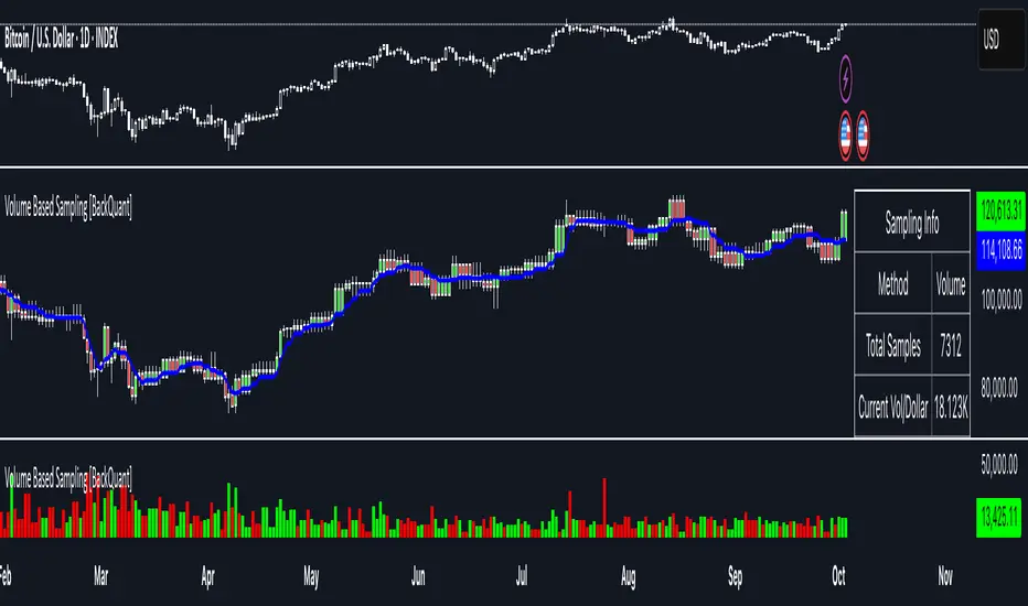
Volume Based Sampling [BackQuant]Volume Based Sampling
What this does
This indicator converts the usual time-based stream of candles into an event-based stream of “synthetic” bars that are created only when enough trading activity has occurred . You choose the activity definition:
Volume bars : create a new synthetic bar whenever the cumulative number of shares/contracts traded reaches a threshold.
Dollar bars : create a new synthetic bar whenever the cumulative traded dollar value (price × volume) reaches a threshold.
The script then keeps an internal ledger of these synthetic opens, highs, lows, closes, and volumes, and can display them as candles, plot a moving average calculated over the synthetic closes, mark each time a new sample is formed, and optionally overlay the native time-bars for comparison.
Why event-based sampling matters
Markets do not release information on a clock: activity clusters during news, opens/closes, and liquidity shocks. Event-based bars normalize for that heteroskedastic arrival of information: during active periods you get more bars (finer resolution); during quiet periods you get fewer bars (coarser resolution). Research shows this can reduce microstructure pathologies and produce series that are closer to i.i.d. and more suitable for statistical modeling and ML. In particular:
Volume and dollar bars are a common event-time alternative to time bars in quantitative research and are discussed extensively in Advances in Financial Machine Learning (AFML). These bars aim to homogenize information flow by sampling on traded size or value rather than elapsed seconds.
The Volume Clock perspective models market activity in “volume time,” showing that many intraday phenomena (volatility, liquidity shocks) are better explained when time is measured by traded volume instead of seconds.
Related market microstructure work on flow toxicity and liquidity highlights that the risk dealers face is tied to information intensity of order flow, again arguing for activity-based clocks.
How the indicator works (plain English)
Choose your bucket type
Volume : accumulate volume until it meets a threshold.
Dollar Bars : accumulate close × volume until it meets a dollar threshold.
Pick the threshold rule
Dynamic threshold : by default, the script computes a rolling statistic (mean or median) of recent activity to set the next bucket size. This adapts bar size to changing conditions (e.g., busier sessions produce more frequent synthetic bars).
Fixed threshold : optionally override with a constant target (e.g., exactly 100,000 contracts per synthetic bar, or $5,000,000 per dollar bar).
Build the synthetic bar
While a bucket fills, the script tracks:
o_s: first price of the bucket (synthetic open)
h_s: running maximum price (synthetic high)
l_s: running minimum price (synthetic low)
c_s: last price seen (synthetic close)
v_s: cumulative native volume inside the bucket
d_samples: number of native bars consumed to complete the bucket (a proxy for “how fast” the threshold filled)
Emit a new sample
Once the bucket meets/exceeds the threshold, a new synthetic bar is finalized and stored. If overflow occurs (e.g., a single native bar pushes you past the threshold by a lot), the code will emit multiple synthetic samples to account for the extra activity.
Maintain a rolling history efficiently
A ring buffer can overwrite the oldest samples when you hit your Max Stored Samples cap, keeping memory usage stable.
Compute synthetic-space statistics
The script computes an SMA over the last N synthetic closes and basic descriptors like average bars per synthetic sample, mean and standard deviation of synthetic returns, and more. These are all in event time , not clock time.
Inputs and options you will actually use
Data Settings
Sampling Method : Volume or Dollar Bars.
Rolling Lookback : window used to estimate the dynamic threshold from recent activity.
Filter : Mean or Median for the dynamic threshold. Median is more robust to spikes.
Use Fixed? / Fixed Threshold : override dynamic sizing with a constant target.
Max Stored Samples : cap on synthetic history to keep performance snappy.
Use Ring Buffer : turn on to recycle storage when at capacity.
Indicator Settings
SMA over last N samples : moving average in synthetic space . Because its index is sample count, not minutes, it adapts naturally: more updates in busy regimes, fewer in quiet regimes.
Visuals
Show Synthetic Bars : plot the synthetic OHLC candles.
Candle Color Mode :
Green/Red: directional close vs open
Volume Intensity: opacity scales with synthetic size
Neutral: single color
Adaptive: graded by how large the bucket was relative to threshold
Mark new samples : drop a small marker whenever a new synthetic bar prints.
Comparison & Research
Show Time Bars : overlay the native time-based candles to visually compare how the two sampling schemes differ.
How to read it, step by step
Turn on “Synthetic Bars” and optionally overlay “Time Bars.” You will see that during high-activity bursts, synthetic bars print much faster than time bars.
Watch the synthetic SMA . Crosses in synthetic space can be more meaningful because each update represents a roughly comparable amount of traded information.
Use the “Avg Bars per Sample” in the info table as a regime signal. Falling average bars per sample means activity is clustering, often coincident with higher realized volatility.
Try Dollar Bars when price varies a lot but share count does not; they normalize by dollar risk taken in each sample. Volume Bars are ideal when share count is a better proxy for information flow in your instrument.
Quant finance background and citations
Event time vs. clock time : Easley, López de Prado, and O’Hara advocate measuring intraday phenomena on a volume clock to better align sampling with information arrival. This framing helps explain volatility bursts and liquidity droughts and motivates volume-based bars.
Flow toxicity and dealer risk : The same authors show how adverse selection risk changes with the intensity and informativeness of order flow, further supporting activity-based clocks for modeling and risk management.
AFML framework : In Advances in Financial Machine Learning , event-driven bars such as volume, dollar, and imbalance bars are presented as superior sampling units for many ML tasks, yielding more stationary features and fewer microstructure distortions than fixed time bars. ( Alpaca )
Practical use cases
1) Regime-aware moving averages
The synthetic SMA in event time is not fooled by quiet periods: if nothing of consequence trades, it barely updates. This can make trend filters less sensitive to calendar drift and more sensitive to true participation.
2) Breakout logic on “equal-information” samples
The script exposes simple alerts such as breakout above/below the synthetic SMA . Because each bar approximates a constant amount of activity, breakouts are conditioned on comparable informational mass, not arbitrary time buckets.
3) Volatility-adaptive backtests
If you use synthetic bars as your base data stream, most signal rules become self-paced : entry and exit opportunities accelerate in fast markets and slow down in quiet regimes, which often improves the realism of slippage and fill modeling in research pipelines (pair this indicator with strategy code downstream).
4) Regime diagnostics
Avg Bars per Sample trending down: activity is dense; expect larger realized ranges.
Return StdDev (synthetic) rising: noise or trend acceleration in event time; re-tune risk.
Interpreting the info panel
Method : your sampling choice and current threshold.
Total Samples : how many synthetic bars have been formed.
Current Vol/Dollar : how much of the next bucket is already filled.
Bars in Bucket : native bars consumed so far in the current bucket.
Avg Bars/Sample : lower means higher trading intensity.
Avg Return / Return StdDev : return stats computed over synthetic closes .
Research directions you can build from here
Imbalance and run bars
Extend beyond pure volume or dollar thresholds to imbalance bars that trigger on directional order flow imbalance (e.g., buy volume minus sell volume), as discussed in the AFML ecosystem. These often further homogenize distributional properties used in ML. alpaca.markets
Volume-time indicators
Re-compute classical indicators (RSI, MACD, Bollinger) on the synthetic stream. The premise is that signals are updated by traded information , not seconds, which may stabilize indicator behavior in heteroskedastic regimes.
Liquidity and toxicity overlays
Combine synthetic bars with proxies of flow toxicity to anticipate spread widening or volatility clustering. For instance, tag synthetic bars that surpass multiples of the threshold and test whether subsequent realized volatility is elevated.
Dollar-risk parity sampling for portfolios
Use dollar bars to align samples across assets by notional risk, enabling cleaner cross-asset features and comparability in multi-asset models (e.g., correlation studies, regime clustering). AFML discusses the benefits of event-driven sampling for cross-sectional ML feature engineering.
Microstructure feature set
Compute duration in native bars per synthetic sample , range per sample , and volume multiple of threshold as inputs to state classifiers or regime HMMs . These features are inherently activity-aware and often predictive of short-horizon volatility and trend persistence per the event-time literature. ( Alpaca )
Tips for clean usage
Start with dynamic thresholds using Median over a sensible lookback to avoid outlier distortion, then move to Fixed thresholds when you know your instrument’s typical activity scale.
Compare time bars vs synthetic bars side by side to develop intuition for how your market “breathes” in activity time.
Keep Max Stored Samples reasonable for performance; the ring buffer avoids memory creep while preserving a rolling window of research-grade data.
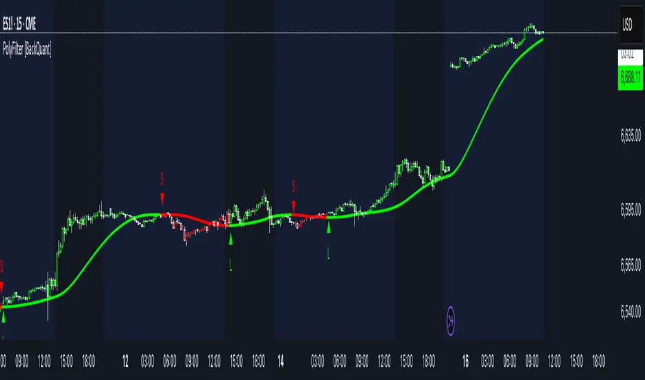
PolyFilter [BackQuant]PolyFilter
A flexible, low-lag trend filter with three smoothing engines—optimized for clean bias, fewer whipsaws, and clear alerting.
What it does
PolyFilter draws a single “intelligent” baseline that adapts to price while suppressing noise. You choose the engine— Fractional MA , Ehlers 2-Pole Super Smoother , or a Multi-Kernel blend . The line can color itself by slope (trend) or by position vs price (above/below), and you get four ready-made alerts for flips and crosses.
What it plots
PolyFilter line — your smoothed trend baseline (width set by “Line Width”).
Optional candle & background coloring — choose: color by trend slope or by whether price is above/below the filter.
Signal markers — Arrows with L/S when the slope flips or when price crosses the line (if you enable shapes/alerts).
How the three engines differ
Fractional MA (experimental) — A power-law weighting of past bars (heavier focus on the most recent samples without throwing away history). The Adaptation Speed acts like the “fraction” exponent (default 0.618). Lower values lean more on recent bars; higher values spread weight further back.
Ehlers 2-Pole Super Smoother — Classic low-lag IIR smoother that aggressively reduces high-frequency noise while preserving turns. Great default when you want a steady, responsive baseline with minimal parameter fuss.
Multi-Kernel — A 70/30 blend of a Gaussian window and an exponential kernel. The Gaussian contributes smooth structure; the exponential adds a hint of responsiveness. Useful for assets that oscillate but still trend.
Reading the colors
Trend mode (default) — Line & candles turn green while the filter is rising (signal > signal ) and red while it’s falling.
Above/Below mode — Line & candles reflect price’s position relative to the filter: green when price > filter, red when price < filter. This is handy if you treat the filter like a dynamic “fair value” or bias line.
Inputs you’ll actually use
Calculation Settings
Price Source — Default HLC/3. Switch to Close for stricter trend, or HLC3/HL2 to soften single-print spikes.
Filter Length — Window/period for all engines. Shorter = snappier turns; longer = smoother line.
Adaptation Speed — Only affects Fractional MA . Lower it for faster, more local weighting; raise it for smoother, more global weighting.
Filter Type — Pick one of: Fractional MA, Ehlers 2-Pole, Multi-Kernel.
UI & Plotting
Color based off… — Choose Trend (slope) or > or < Close (position vs price).
Long/Short Colors — Customize bull/bear hues to your theme.
Show Filter Line / Paint candles / Color background — Visual toggles for the line, bars, and backdrop.
Line Width — Make the filter stand out (2–3 works well on most charts).
Signals & Alerts
PolyFilter Trend Up — Slope flips upward (the filter crosses above its prior value). Good for early continuation entries or stop-tightening on shorts.
PolyFilter Trend Down — Slope flips downward. Often used to scale out longs or rotate bias.
PolyFilter Above Price — The filter line crosses up through price (filter > price). This can confirm that mean has “caught up” after a pullback.
PolyFilter Below Price — The filter line crosses down through price (filter < price). Useful to confirm momentum loss on bounces.
Quick starts (suggested presets)
Intraday (5–15m, crypto or indices) — Ehlers 2-Pole, Length 55–80. Trend coloring ON, candle paint ON. Look for pullbacks to a rising filter; avoid fading a falling one.
Swing (1H–4H) — Multi-Kernel, Length 80–120. Background color OFF (cleaner), candle paint ON. Add a higher-TF confirmation (e.g., 4H filter rising when you trade 1H).
Range-prone FX — Fractional MA, Length 70–100, Adaptation ~0.55–0.70. Consider Above/Below mode to trade mean reversion to the line with a strict risk cap.
How to use it in practice
Bias line — Trade in the direction of the filter slope; stand aside when it flattens and color chops back and forth.
Dynamic support/resistance — Treat the line as a moving value area. In trends, entries often appear on shallow tags of the line with structure confluence.
Regime switch — When the filter flips and holds color for several bars, tighten stops on the opposing side and look for first pullback in the new color.
Stacking filters — Many users run PolyFilter on the active chart and a slower instance (longer length) on a higher timeframe as a “macro bias” guardrail.
Tuning tips
If you see too many flips, lengthen the filter or switch to Multi-Kernel.
If turns feel late, shorten the filter or try Ehlers 2-Pole for lower lag.
On thin or very noisy symbols, prefer HLC3 as the source and longer lengths.
Performance note: very large lengths increase computation time for the Multi-Kernel and Fractional engines. Start moderate and scale up only if needed.
Summary
PolyFilter gives you a single, trustworthy baseline that you can read at a glance—either as a pure trend line (slope coloring) or as a dynamic “above/below fair value” reference. Pick the engine that matches your market’s personality, set a sensible length, and let the color and alerts guide bias, entries on pullbacks, and risk on reversals.
Algorithmic Kalman Filter [CRYPTIK1]Price action is chaos. Markets are driven by high-frequency algorithms, emotional reactions, and raw speculation, creating a constant stream of noise that obscures the true underlying trend. A simple moving average is too slow, too primitive to navigate this environment effectively. It lags, it gets chopped up, and it fails when you need it most.
This script implements an Algorithmic Kalman Filter (AKF), a sophisticated signal processing algorithm adapted from aerospace and robotic guidance systems. Its purpose is singular: to strip away market noise and provide a hyper-adaptive, self-correcting estimate of an asset's true trajectory.
The Concept: An Adaptive Intelligence
Unlike a moving average that mindlessly averages past data, the Kalman Filter operates on a two-step principle: Predict and Update.
Predict: On each new bar, the filter makes a prediction of the true price based on its previous state.
Update: It then measures the error between its prediction and the actual closing price. It uses this error to intelligently correct its estimate, learning from its mistakes in real-time.
The result is a flawlessly smooth line that adapts to volatility. It remains stable during chop and reacts swiftly to new trends, giving you a crystal-clear view of the market's real intention.
How to Wield the Filter: The Core Settings
The power of the AKF lies in its two tuning parameters, which allow you to calibrate the filter's "brain" to any asset or timeframe.
Process Noise (Q) - Responsiveness: This controls how much you expect the true trend to change.
A higher Q value makes the filter more sensitive and responsive to recent price action. Use this for highly volatile assets or lower timeframes.
A lower Q value makes the filter smoother and more stable, trusting that the underlying trend is slow-moving. Use this for higher timeframes or ranging markets.
Measurement Noise (R) - Smoothness: This controls how much you trust the incoming price data.
A higher R value tells the filter that the price is extremely noisy and to be more skeptical. This results in a much smoother, slower-moving line.
A lower R value tells the filter to trust the price data more, resulting in a line that tracks price more closely.
The interaction between Q and R is what gives the filter its power. The default settings provide a solid baseline, but a true operator will fine-tune these to perfectly match the rhythm of their chosen market.
Tactical Application
The AKF is not just a line; it's a complete framework for viewing the market.
Trend Identification: The primary signal. The filter's color code provides an unambiguous definition of the trend. Teal for an uptrend, Pink for a downtrend. No more guesswork.
Dynamic Support & Resistance: The filter itself acts as a dynamic level. Watch for price to pull back and find support on a rising (Teal) filter in an uptrend, or to be rejected by a falling (Pink) filter in a downtrend.
A Higher-Order Filter: Use the AKF's trend state to filter signals from your primary strategy. For example, only take long signals when the AKF is Teal. This single rule can dramatically reduce noise and eliminate low-probability trades.
This is a professional-grade tool for traders who are serious about gaining a statistical edge. Ditch the lagging averages. Extract the signal from the noise.

Theil-Sen Line Filter [BackQuant]Theil-Sen Line Filter
A robust, median-slope baseline that tracks price while resisting outliers. Designed for the chart pane as a clean, adaptive reference line with optional candle coloring and slope-flip alerts.
What this is
A trend filter that estimates the underlying slope of price using a Theil-Sen style median of past slopes, then advances a baseline by a controlled fraction of that slope each bar. The result is a smooth line that reacts to real directional change while staying calm through noise, gaps, and single-bar shocks.
Why Theil-Sen
Classical moving averages are sensitive to outliers and shape changes. Ordinary least squares is sensitive to large residuals. The Theil-Sen idea replaces a single fragile estimate with the median of many simple slopes, which is statistically robust and less influenced by a few extreme bars. That makes the baseline steadier in choppy conditions and cleaner around regime turns.
What it plots
Filtered baseline that advances by a fraction of the robust slope each bar.
Optional candle coloring by baseline slope sign for quick trend read.
Alerts when the baseline slope turns up or down.
How it behaves (high level)
Looks back over a fixed window and forms many “current vs past” bar-to-bar slopes.
Takes the median of those slopes to get a robust estimate for the bar.
Optionally caps the magnitude of that per-bar slope so a single volatile bar cannot yank the line.
Moves the baseline forward by a user-controlled fraction of the estimated slope. Lower fractions are smoother. Higher fractions are more responsive.
Inputs and what they do
Price Source — the series the filter tracks. Typical is close; HL2 or HLC3 can be smoother.
Window Length — how many bars to consider for slopes. Larger windows are steadier and slower. Smaller windows are quicker and noisier.
Response — fraction of the estimated slope applied each bar. 1.00 follows the robust slope closely; values below 1.00 dampen moves.
Slope Cap Mode — optional guardrail on each bar’s slope:
None — no cap.
ATR — cap scales with recent true range.
Percent — cap scales with price level.
Points — fixed absolute cap in price points.
ATR Length / Mult, Cap Percent, Cap Points — tune the chosen cap mode’s size.
UI Settings — show or hide the line, paint candles by slope, choose long and short colors.
How to read it
Up-slope baseline and green candles indicate a rising robust trend. Pullbacks that do not flip the slope often resolve in trend direction.
Down-slope baseline and red candles indicate a falling robust trend. Bounces against the slope are lower-probability until proven otherwise.
Flat or frequent flips suggest a range. Increase window length or decrease response if you want fewer whipsaws in sideways markets.
Use cases
Bias filter — only take longs when slope is up, shorts when slope is down. It is a simple way to gate faster setups.
Stop or trail reference — use the line as a trailing guide. If price closes beyond the line and the slope flips, consider reducing exposure.
Regime detector — widen the window on higher timeframes to define major up vs down regimes for asset rotation or risk toggles.
Noise control — enable a cap mode in very volatile symbols to retain the line’s continuity through event bars.
Tuning guidance
Quick swing trading — shorter window, higher response, optionally add a percent cap to keep it stable on large moves.
Position trading — longer window, moderate response. ATR cap tends to scale well across cycles.
Low-liquidity or gappy charts — prefer longer window and a points or ATR cap. That reduces jumpiness around discontinuities.
Alerts included
Theil-Sen Up Slope — baseline’s one-bar change crosses above zero.
Theil-Sen Down Slope — baseline’s one-bar change crosses below zero.
Strengths
Robust to outliers through median-based slope estimation.
Continuously advances with price rather than re-anchoring, which reduces lag at turns.
User-selectable slope caps to tame shock bars without over-smoothing everything.
Minimal visuals with optional candle painting for fast regime recognition.
Notes
This is a filter, not a trading system. It does not account for execution, spreads, or gaps. Pair it with entry logic, risk management, and higher-timeframe context if you plan to use it for decisions.

Deadband Hysteresis Filter [BackQuant]Deadband Hysteresis Filter
What this is
This tool builds a “debounced” price baseline that ignores small fluctuations and only reacts when price meaningfully departs from its recent path. It uses a deadband to define how much deviation matters and a hysteresis scheme to avoid rapid flip-flops around the decision boundary. The baseline’s slope provides a simple trend cue, used to color candles and to trigger up and down alerts.
Why deadband and hysteresis help
They filter micro noise so the baseline does not react to every tiny tick.
They stabilize state changes. Hysteresis means the rule to start moving is stricter than the rule to keep holding, which reduces whipsaw.
They produce a stepped, readable path that advances during sustained moves and stays flat during chop.
How it works (conceptual)
At each bar the script maintains a running baseline dbhf and compares it to the input price p .
Compute a base threshold baseTau using the selected mode (ATR, Percent, Ticks, or Points).
Build an enter band tauEnter = baseTau × Enter Mult and an exit band tauExit = baseTau × Exit Mult where typically Exit Mult < Enter Mult .
Let diff = p − dbhf .
If diff > +tauEnter , raise the baseline by response × (diff − tauEnter) .
If diff < −tauEnter , lower the baseline by response × (diff + tauEnter) .
Otherwise, hold the prior value.
Trend state is derived from slope: dbhf > dbhf → up trend, dbhf < dbhf → down trend.
Inputs and what they control
Threshold mode
ATR — baseTau = ATR(atrLen) × atrMult . Adapts to volatility. Useful when regimes change.
Percent — baseTau = |price| × pctThresh% . Scale-free across symbols of different prices.
Ticks — baseTau = syminfo.mintick × tickThresh . Good for futures where tick size matters.
Points — baseTau = ptsThresh . Fixed distance in price units.
Band multipliers and response
Enter Mult — outer band. Price must travel at least this far from the baseline before an update occurs. Larger values reject more noise but increase lag.
Exit Mult — inner band for hysteresis. Keep this smaller than Enter Mult to create a hold zone that resists small re-entries.
Response — step size when outside the enter band. Higher response tracks faster; lower response is smoother.
UI settings
Show Filtered Price — plots the baseline on price.
Paint candles — colors bars by the filtered slope using your long/short colors.
How it can be used
Trend qualifier — take entries only in the direction of the baseline slope and skip trades against it.
Debounced crossovers — use the baseline as a stabilized surrogate for price in moving-average or channel crossover rules.
Trailing logic — trail stops a small distance beyond the baseline so small pullbacks do not eject the trade.
Session aware filtering — widen Enter Mult or switch to ATR mode for volatile sessions; tighten in quiet sessions.
Parameter interactions and tuning
Enter Mult vs Response — both govern sensitivity. If you see too many flips, increase Enter Mult or reduce Response. If turns feel late, do the opposite.
Exit Mult — widening the gap between Enter and Exit expands the hold zone and reduces oscillation around the threshold.
Mode choice — ATR adapts automatically; Percent keeps behavior consistent across instruments; Ticks or Points are useful when you think in fixed increments.
Timeframe coupling — on higher timeframes you can often lower Enter Mult or raise Response because raw noise is already reduced.
Concrete starter recipes
General purpose — ATR mode, atrLen=14 , atrMult=1.0–1.5 , Enter=1.0 , Exit=0.5 , Response=0.20 . Balanced noise rejection and lag.
Choppy range filter — ATR mode, increase atrMult to 2.0, keep Response≈0.15 . Stronger suppression of micro-moves.
Fast intraday — Percent mode, pctThresh=0.1–0.3 , Enter=1.0 , Exit=0.4–0.6 , Response=0.30–0.40 . Quicker turns for scalping.
Futures ticks — Ticks mode, set tickThresh to a few spreads beyond typical noise; start with Enter=1.0 , Exit=0.5 , Response=0.25 .
Strengths
Clear, explainable logic with an explicit noise budget.
Multiple threshold modes so the same tool fits equities, futures, and crypto.
Built-in hysteresis that reduces flip-flop near the boundary.
Slope-based coloring and alerts that make state changes obvious in real time.
Limitations and notes
All filters add lag. Larger thresholds and smaller response trade faster reaction for fewer false turns.
Fixed Points or Ticks can under- or over-filter when volatility regime shifts. ATR adapts, but will also expand bands during spikes.
On extremely choppy symbols, even a well tuned band will step frequently. Widen Enter Mult or reduce Response if needed.
This is a chart study. It does not include commissions, slippage, funding, or gap risks.
Alerts
DBHF Up Slope — baseline turns from down to up on the latest bar.
DBHF Down Slope — baseline turns from up to down on the latest bar.
Implementation details worth knowing
Initialization sets the baseline to the first observed price to avoid a cold-start jump.
Slope is evaluated bar-to-bar. The up and down alerts check for a change of slope rather than raw price crossings.
Candle colors and the baseline plot share the same long/short palette with transparency applied to the line.
Practical workflow
Pick a mode that matches how you think about distance. ATR for volatility aware, Percent for scale-free, Ticks or Points for fixed increments.
Tune Enter Mult until the number of flips feels appropriate for your timeframe.
Set Exit Mult clearly below Enter Mult to create a real hold zone.
Adjust Response last to control “how fast” the baseline chases price once it decides to move.
Final thoughts
Deadband plus hysteresis gives you a principled way to “only care when it matters.” With a sensible threshold and response, the filter yields a stable, low-chop trend cue you can use directly for bias or plug into your own entries, exits, and risk rules.

♨️盛天®MACD背離Ⓜ️速效TopDog版🕯📊功能概述
該指標整合了傳統 MACD(移動平均線收斂-發散指標)的核心功能,並新增了背離檢測、Top Dog Trading 的 MOM 和 DAD 模式、多時間框架支持以及靈活的視覺化和警報設置。
以下是其主要功能👇 :
1️⃣ MACD 核心計算MACD 線:由快速移動平均線(Fast MA)減去慢速移動平均線(Slow MA)計算得出,反映價格的短期與長期趨勢差異。
信號線:對 MACD 線進行平滑處理(通常使用 EMA 或 SMA),用於識別趨勢轉換點。
直方圖:MACD 線與信號線的差值,顯示動量的強弱和方向。
靈活性:用戶可選擇使用 EMA(指數移動平均線)或 SMA(簡單移動平均線)進行計算,並可設置快速均線、慢速均線和信號線的週期。
📊Feature Overview
This indicator integrates the core functionality of the traditional MACD (Moving Average Convergence-Divergence) indicator and adds divergence detection, Top Dog Trading's MOM and DAD modes, support for multiple time frames, and flexible visualization and alert settings.
Here are its key features:
1. MACD Core Calculation: The MACD Line is calculated by subtracting the Slow Moving Average (Slow MA) from the Fast Moving Average (Fast MA) and reflects the divergence between short-term and long-term price trends.
Signal Line: The MACD Line is smoothed (typically using an EMA or SMA) to identify trend reversals.
Histogram: The difference between the MACD Line and the Signal Line indicates the strength and direction of momentum.
Flexibility: Users can choose to use either EMA (Exponential Moving Average) or SMA (Simple Moving Average) for calculations, and can set the periods for the fast and slow moving averages, as well as the signal line.
2️⃣多時間框架支持通過 request.security 函數,允許用戶選擇不同的時間框架(例如 1 小時、日線等)來計算 MACD,適用於分析更高或更低時間框架的趨勢,無需改變圖表的當前時間框架。
2️⃣Multi-timeframe support is available through the request.security function, allowing users to select different timeframes (such as 1 hour, daily, etc.) to calculate the MACD. This is suitable for analyzing trends in higher or lower timeframes without changing the current timeframe of the chart.
3️⃣Top Dog Mode:
The Top Dog Mode is an advanced feature of the indicator that enhances the MACD's sensitivity to short-term momentum and its ability to identify long-term trends through specific moving average periods (5, 20, 30) and MOM/DAD visualization. It is particularly suitable for short-term traders, swing traders, and market participants who need fast momentum signals. Through crossover dots, MOM histograms, DAD direction alerts, and divergence detection, the Top Dog Mode provides traders with flexible signal generation tools suitable for various market environments.
The signal line period (30) is longer than the standard MACD's 9, which helps filter out short-term fluctuations and confirm long-term trends.
The Top Dog pattern is suitable for the following trading scenarios:
(🔵➤ Short-term trading scenario: In highly volatile markets (such as forex or cryptocurrencies), use the rapid crossover signals of the MOM and DAD to capture short-term price fluctuations.
Recommendation: Use this pattern on lower timeframes (such as the 5-minute or 15-minute timeframe) and set a stop-loss to control risk.
(🔵➤ Trend confirmation scenario: Use the direction of the DAD to confirm the long-term trend and combine it with the MOM histogram to determine entry points.
Recommendation: Use this pattern on higher timeframes (such as the 1-hour or 4-hour timeframe) and combine it with trendlines or moving averages.
(🔵➤ Reversal trading scenario: Combine the Top Dog pattern's divergence signals (labeled "divergence" or "hidden") to identify potential trend reversals.
Recommendation: Confirm divergence signals near key support/resistance levels to reduce the risk of false positives.
(🔵➤ Trend Continuation Scenarios: Using Hidden Divergences (labeled "Hidden") to Identify Trend Continuation Opportunities 👇
4. Divergence Detection: Regular Divergences (labeled "Divergence"): Bullish Divergence: When the price makes lower lows, but the MACD histogram or MACD line makes higher lows, it indicates weakening bearish momentum and may signal a reversal.
Bearish Divergence: When the price makes higher highs, but the MACD histogram or MACD line makes lower highs, it indicates weakening bullish momentum and may signal a reversal. 👇
Hidden Divergences (labeled "Hidden"): Hidden Bullish Divergence: When the price makes higher lows, but the MACD histogram or MACD line makes lower lows, it may signal the possibility of trend continuation.
Hidden Bearish Divergence: When the price makes lower highs, but the MACD histogram or MACD line makes lower highs, it may signal a reversal. The line has made a higher high, indicating the possibility of trend continuation👇
3️⃣Top Dog 模式:
Top Dog 模式是該指標的一個進階功能,通過特定的均線週期(5、20、30)和 MOM/DAD 的視覺化方式,增強了 MACD 對短期動量的敏感性和長期趨勢的確認能力。它特別適合短線交易者、波段交易者和需要快速動量信號的市場參與者。通過交叉圓點、MOM 直方圖、DAD 方向警報和背離檢測,Top Dog 模式為交易者提供了靈活的信號生成工具,適用於多種市場環境。
信號線週期(30)比標準 MACD 的 9 更長,有助於過濾短期波動,確認長期趨勢。
Top Dog 模式適用於以下交易場景:
(🔵➤短線交易場景:在高波動市場(如外匯或加密貨幣)中,利用 MOM 和 DAD 的快速交叉信號捕捉短期價格波動。
建議:在低時間框架(如 5 分鐘或 15 分鐘)使用,並設置止損以控制風險。
(🔵➤ 趨勢確認場景:利用 DAD 的方向確認長期趨勢,結合 MOM 直方圖判斷進場時機。
建議:在較高時間框架(如 1 小時或 4 小時)使用,結合趨勢線或移動平均線。
(🔵➤反轉交易場景:結合 Top Dog 模式的背離信號(標籤“背”或“隱”),識別潛在的趨勢反轉。
建議:在關鍵支撐/阻力位附近確認背離信號,降低假信號風險。
(🔵➤ 趨勢延續場景:利用隱藏背離(標籤“隱”)捕捉趨勢延續機會👇
4. Divergence Detection: Regular Divergence (labeled "Divergence"): Bullish Divergence: When prices make lower lows, but the MACD histogram or MACD line makes higher lows, it indicates weakening downside momentum and may signal a reversal.
Bearish Divergence: When prices make higher highs, but the MACD histogram or MACD line makes lower highs, it indicates weakening upside momentum and may signal a reversal.
4️⃣背離檢測常規背離(標籤為“背”):看漲背離:當價格創出更低低點,但 MACD 直方圖或 MACD 線創出更高低點,表明下跌動量減弱,可能預示反轉。
看跌背離:當價格創出更高高點,但 MACD 直方圖或 MACD 線創出更低高點,表明上漲動量減弱,可能預示反轉👇。
隱藏背離(標籤為“隱”):隱藏看漲背離:當價格創出更高低點,但 MACD 直方圖或 MACD 線創出更低低點,表明趨勢延續的可能。
隱藏看跌背離:當價格創出更低高點,但 MACD 直方圖或 MACD 線創出更高高點,表明趨勢延續的可能👇
5️⃣ Trend Coloring MACD Line: Based on the position of the MACD line relative to the signal line (crossing above for an uptrend, crossing below for a downtrend), you can choose whether to display the trend color (default green for uptrend, red for downtrend)👇.
5️⃣ 趨勢著色MACD 線:根據 MACD 線相對於信號線的位置(上穿為上升趨勢,下穿為下降趨勢),可選擇是否顯示趨勢顏色(默認綠色為上升,紅色為下降)👇 。
6️⃣ Crossover Dots:
When the MACD line crosses the signal line, a dot appears: Upward crossover (MACD line crosses above the signal line): a green dot.
Downward crossover (MACD line crosses below the signal line): a red dot. You can set whether to display the dot and its width.
6️⃣ 交叉圓點:
當 MACD 線與信號線交叉時,顯示圓點:上穿(MACD 線上穿信號線):綠色圓點。
下穿(MACD 線下穿信號線):紅色圓點。可設置是否顯示以及寬度👇 。
7️⃣ Display Flexibility: Users can choose whether to display the MACD line, signal line, histogram, histogram outline, MOM histogram (Top Dog pattern), crossover dots, and divergence labels.
Line widths (MACD line, signal line, histogram, dots) and color settings are adjustable.
7️⃣顯示靈活性用戶可選擇是否顯示 MACD 線、信號線、直方圖、直方圖外框、MOM 直方圖(Top Dog 模式)、交叉圓點和背離標籤。
可調整線條寬度(MACD 線、信號線、直方圖、圓點)和顏色設置👇 。
8️⃣警報功能:
MACD交叉警報:
🚨MACD 線上穿信號線(看漲信號)。
🚨MACD 線下穿信號線(看跌信號)。
🚨MACD > 0 且上穿(強看漲信號)。
🚨MACD < 0 且下穿(強看跌信號)。
背離警報:
🚨MACD 直方圖/MOM 的常規和隱藏看漲/看跌背離。
🚨MACD 線/DAD 的常規和隱藏看漲/看跌背離。
DAD 方向警報:
🚨DAD(信號線)方向改變(交叉前一根 K 線的信號線值)。
🚨DAD 向上(信號線上升)。
🚨DAD 向下(信號線下降)。
所有警報默認啟用,可通過 TradingView 的警報設置面板配置通知方式。
8️⃣Alert Features:
MACD Crossover Alerts:
🚨MACD Line crosses above Signal Line (bullish signal).
🚨MACD Line crosses below Signal Line (bearish signal).
🚨MACD > 0 and crosses upward (strong bullish signal).
🚨MACD < 0 and crosses downward (strong bearish signal).
Divergence Alerts:
🚨Regular and hidden bullish/bearish divergences of the MACD Histogram/MOM.
🚨Regular and hidden bullish/bearish divergences of the MACD Line/DAD.
DAD Direction Alerts:
🚨DAD (Signal Line) direction changes (crosses over the previous candlestick's Signal Line value).
🚨DAD up (Signal Line rising).
🚨DAD down (Signal Line falling).
All alerts are enabled by default, and notification methods can be configured through the TradingView Alerts panel.
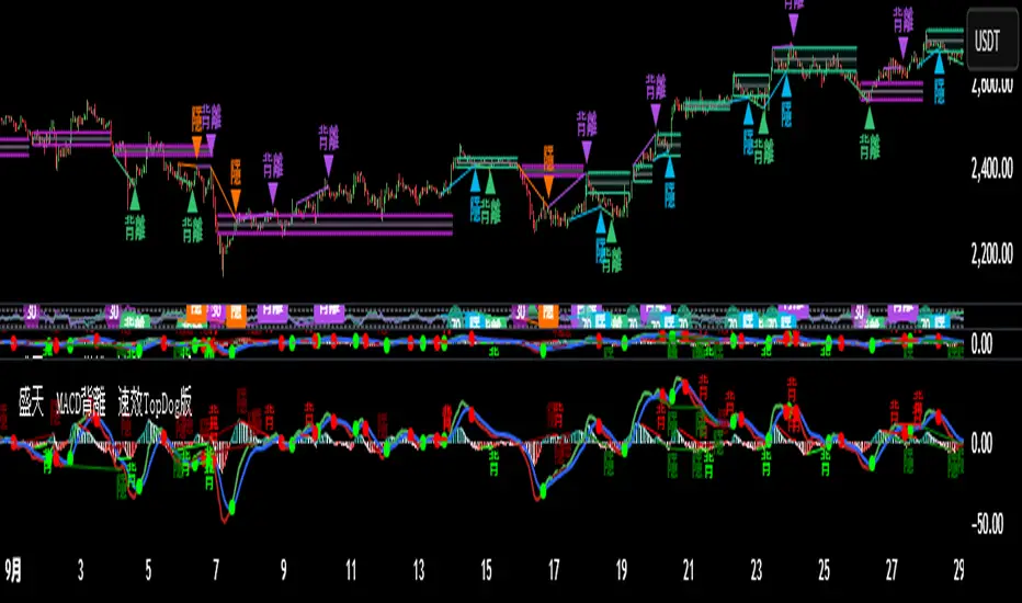
Kalman Filter (Smoothed)The Kalman Filter is a recursive statistical algorithm that smooths noisy price data while adapting dynamically to new information. Unlike simple moving averages or EMAs, it minimizes lag by balancing measurement noise (R) and process noise (Q), giving traders a clean, adaptive estimate of true price action.
🔹 Core Features
Real-time recursive estimation
Adjustable noise parameters (R = sensitivity to price, Q = smoothness vs. responsiveness)
Reduces market noise without heavy lag
Overlay on chart for direct comparison with raw price
🔹 Trading Applications
Smoother trend visualization compared to traditional MAs
Spotting true direction during volatile/sideways markets
Filtering out market “whipsaws” for cleaner signals
Building blocks for advanced quant/trading models
⚠️ Note: The Kalman Filter is a state-space model; it doesn’t predict future price, but smooths past and present data into a more reliable signal.
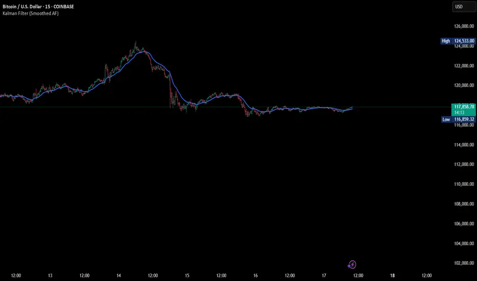
The Oracle by JaeheeThe Oracle
Summary
The Oracle is a volatility-adaptive trend indicator built on a smoothed range filter, persistence counters, and regime-flip logic. Signals appear only when price establishes a sustained move and flips from one regime to the other. An EMA(50)-anchored ribbon provides a flowing visual context but does not drive signals.
What it does
① Calculates a smoothed volatility-based range to adapt to market conditions
② Builds a filtered price path that reduces single-bar noise
③ Tracks persistence of upward or downward filter movement with counters
④ Confirms Buy/Sell signals only on regime flips, not on single ticks
⑤ Draws a multi-phase ribbon around EMA(50) to visualize slope and bias
How it works (concept level)
① Smoothed Range: Double EMA of absolute price change, scaled by multiplier
② Filtered Price: Range filter constrains price movement to reduce noise
③ Persistence Counters: Upward/Downward counters accumulate only if the filter continues in one direction
④ Signal Logic:
• Buy = price above filter AND prior regime was short
• Sell = price below filter AND prior regime was long
• Requires a full flip of state to confirm new signals
⑤ Ribbon: EMA(50) baseline with sinusoidal offsets creates a flowing ribbon, colored by EMA slope (visual only)
Why it is useful
① Noise resistance: Avoids whipsaws by requiring persistence + state flips
② Clarity: Ribbon visually encodes background trend for quick recognition
③ Balanced design: Combines volatility adaptation, persistence, and confirmation in one framework
④ Adaptable: Works across assets and timeframes without heavy parameter tuning
How to use it
① Signal reading:
• ✧ Buy marker = confirmed transition into an upward regime
• ✧ Sell marker = confirmed transition into a downward regime
• Use bar close confirmation
② Ribbon context: Align trades with ribbon slope/color to stay with the dominant trend
③ Timeframes:
• Higher (4H, Daily) = better swing bias
• Lower (5m, 15m) = faster signals but noisier
④ Combination: Pair with ATR stops, position sizing, or volume/momentum studies for added confirmation
Limitations
① Still possible to see false flips in choppy consolidations
② Smoothing introduces slight delay in regime confirmation
③ Signals can repaint intrabar — confirm on bar close
④ Indicator only — no built-in money management or strategy logic
Best Practices (Recommended Use)
① Confirm on bar close
• Signals can change intrabar; always make decisions after the bar has closed.
② Validate across multiple timeframes
• Although the tool adapts to volatility, reliability improves on higher timeframes.
• In practice, the 1-hour chart has shown the most stable balance between reactivity and noise.
③ Align with ribbon bias
• Trade in the same direction as the ribbon slope/color to reduce countertrend exposure.
④ Combine with independent risk management
• Use stop-losses, position sizing, or ATR-based targets outside the script.
• The indicator highlights transitions, but risk control must be user-defined.
⑤ Use as confirmation, not prediction
• Treat signals as confirmation of regime change, not as a forecast of future price.
[Pandora][Swarm] Rapid Exponential Moving AverageENVISIONING POSSIBILITY
What is the theoretical pinnacle of possibility? The current state of algorithmic affairs falls far short of my aspirations for achievable feasibility. I'm lifting the lid off of Pandora's box once again, very publicly this time, as a brute force challenge to conventional 'wisdom'. The unfolding series of time mandates a transcendental systemic alteration...
THE MOVING AVERAGE ZOO:
The realm of digital signal processing for trading is filled with familiar antiquated filtering tools. Two families of filtration, being 'infinite impulse response' (EMA, RMA, etc.) and 'finite impulse response' (WMA, SMA, etc.), are prevalently employed without question. These filter types are the mules and donkeys of data analysis, broadly accepted for use in finance.
At first glance, they appear sufficient for most tasks, offering a basic straightforward way to reduce noise and highlight trends. Yet, beneath their simplistic facade lies a constellation of limitations and impediments, each having its own finicky quirks. Upon closer inspection, identifiable drawbacks render them far from ideal for many real-world applications in today's volatile markets.
KNOWN FUNDAMENTAL FLAWS:
Despite commonplace moving average (MA) popularity, these conventional filters suffer from an assortment of fundamental flaws. Most of them don't genuinely address core challenges of how to preserve the true dynamics of a signal while suppressing noise and retaining cutoff frequency compliance. Their simple cookie cutter structures make them ill-suited in actuality for dynamic market environments. In reality, they often trade one problem for another dilemma, forsaking analytics to choose between distortion and delay.
A deeper seeded issue remains within frequency compliance, how adequately a filter respects (or disrespects) the underlying signal’s spectral properties according to it's assigned periodic parameter. Traditional MAs habitually distort phase relationships, causing delayed reactions with surplus lag or exaggerations with excessive undershoot/overshoot. For applications requiring timely resilience, such as algorithmic trading, these shortcomings are often functionally unacceptable. What’s needed is vigorous filters that can more accurately retain signal behaviors while minimizing lag without sacrificing smoothness and uniformity. Until then, the public MA zoo remains as a collection of corny compromises, rather than a favorable toolbelt of solutions.
P.S.: In PSv7+, in my opinion, many of these geriatric MAs deserve no future with ease of access for the naive, simply not knowing these filters are most likely creating bigger problems than solving any.
R.E.M.A.
What is this? I prefer to think of it as the "radical EMA", definitely along my lines of a retire everything morte algorithm. This isn't your run of the mill average from the petting zoo. I would categorize it as a paradigm shifting rampant economic masochistic annihilator, sufficiently good enough to begin ruthlessly executing moving averages left and right. Um, yeah... that kind of moving average destructor as you may soon recognize with a few 'Filters+' settings adjustments, realizing ordinary EMA has been doing us an injustice all this time.
Does it possess the capability to relentlessly exterminate most averaging filters in existence? Well, it's about time we find out, by uncaging it on the loose into the greater economic wilderness. Only then can we truly find out if it is indeed a radical exponential market accelerant whose time has come. If it is, then it may eventually become a reality erasing monolithic anomaly destined for greatness, ultimately changing the entire landscape of trading in perpetuity.
UNLEASHING NEXT-GEN:
This lone next generation exoweapon algorithm is intended to initiate the transformative beginning stages of mass filtration deprecation. However, it won't be the only one, just the first arrival of it's alien kind from me. Welcome to notion #1 of my future filtration frontier, on this episode of the algorithmic twilight zone. Where reality takes a twisting turn one dimension beyond practical logic, after persistent models of mindset disintegrate into insignificance, followed by illusory perception confronted into cognitive dissonance.
An evolutionary path to genuine advancement resides outside the prison of preconceptions, manifesting only after divergence from persistent binding restrictions of dogmatic doctrines. Such a genesis in transformative thinking will catalyze unbounded cognitive potential, plowing the way for the cultivation of total redesigns of thought. Futuristic innovative breakthroughs demand the surrender of legacy and outmoded understandings.
Now that the world's largest assembly of investors has been ensembled, there are additional tasks left to perform. I'm compelled to deploy this mathematical-weapon of mass financial creation into it's rightful destined hands, to "WE THE PEOPLE" of TV.
SCRIPT INTENTION:
Deprecate anything and everything as any non-commercial member sees desirably fit. This includes your existing code formulations already in working functional modes of operation AND/OR future projects in the works. Swapping is nearly as simple as copying and pasting with meager modifications, after you have identified comparable likeness in this indicators settings with a visual assessment. Results may become eye opening, but only if you dare to look and test.
Where you may suspect a ta.filter() is lacking sufficient luster or may be flat out majorly deficient, employing rema, drema, trema, or qrema configurations may be a more suitable replacement. That's up to you to discern. My code satire already identifies likely bottom of the barrel suspects that either belong in the extinction record or have already been marked for deprecation. They are ordered more towards the bottom by rank where they belong. SuperSmoother is a masterpiece here to stay, being my original go-to reference filter. Everything you see here is already deprecated, including REMA...
REMA CHARACTERISTICS
- VERY low lag
- No overshoot
- Frequency compliant
- Proper initialization at bar_index==0
- Period parameter accepts poitive floating point numerics (AND integers!)
- Infinite impulse response (IIR) filter
- Compact code footprint
- Minimized computational overhead
Mayfair Reversal Change✅ Mayfair Reversal Change — By EastWave Capital
Description:
The Mayfair Reversal Change indicator is a tool designed to help traders identify potential market turning points using Stochastic Oscillator behavior and filtered price action logic. It acts as a reversal signal filter and is particularly effective when the market is overextended (overbought/oversold) and about to revert from exhaustion zones.
🔍 How It Works:
This script monitors the Stochastic %K and %D crossovers and adds a custom logic layer to filter only high-quality reversal points:
Stochastic Filter Conditions:
Uses smoothed stochastic settings:
%K smoothing = 3
%D smoothing = 3
Only shows signals after %K crosses back below 80 (for Sell) or above 20 (for Buy)
This prevents signals from appearing too early during an active overbought or oversold phase.
Directional Confirmation Logic:
Bullish signal is printed only when %K re-enters below 20 after a confirmed stochastic crossover.
Bearish signal appears only when %K re-enters above 80.
This reduces false signals that occur during continued trending moves.
Toggle Switch:
A user-toggle input is included to enable or disable the reversal filter logic.
This gives flexibility for traders who want to test signals with or without the stochastic condition.
📈 How to Use:
Timeframes: Recommended for 5M, 15M, and 30M
Markets: Compatible with any market — FX, Gold, Indices, Crypto
Entry Approach:
Wait for signal after price has reached a potential extreme area.
Confirm with chart structure, support/resistance, or SMC zone.
Enter on confirmation, placing stop loss beyond the swing high/low.
Combine with trendline breaks or price imbalances (FVG) for extra confluence.
Can be used in combination with the Mayfair FX Scalper script for dual-layer confirmation.
⚠️ Important Notes:
Signals are visual only and should be confirmed with proper strategy.
This indicator does not execute or manage trades automatically.
Designed to assist with reversal setups but should not be used in isolation.
Always manage risk, use SL/TP, and avoid over-leveraging.

Combo 2/20 EMA & Bandpass Filter by TamarokDescription:
This strategy combines a 2/20 exponential moving average (EMA) crossover with a custom bandpass filter to generate buy and sell signals.
Use the Fast EMA and Slow EMA inputs to adjust trend sensitivity, and the Bandpass Filter Length, Delta, and Zones to fine-tune momentum turns.
Signals occur when both EMA and BPF agree in direction, with optional reversal and time filters.
How to use:
1. Add the script to your chart in TradingView.
2. Adjust the EMA and BP Filter parameters to match your asset’s volatility.
3. Enable ‘Reverse Signals’ to trade counter-trend, or use the time filter to limit sessions.
4. Set alerts on Long Alert and Short Alert for automated notifications.
Inspiration:
Based on HPotter’s original combo strategy (Stocks & Commodities Mar 2010).
Updated to Pine Script v6 with streamlined code and alerts.
WARNING:
For purpose educate only
