Markovchain — Indicators and Strategies

JINN: A Multi-Paradigm Quantitative Trading and Execution Engine I. Core Philosophy: A Substitute for Static Analysis JINN (Joint Investment Neural and Network) represents a paradigm shift from static indicators to a living, adaptive analytical ecosystem. Traditional tools provide a fixed snapshot of the market. JINN operates on a fundamentally different premise: it treats the market as a dynamic, regime-driven system. It processes market data through a hierarchical suite of advanced, interacting models, arbitrates their outputs through a rules-based engine, and adapts its own logic in real-time. It is designed as a complete framework for traders who think in terms of statistical edge, market regimes, probabilistic outcomes, and adaptive risk management. II. The JINN Branded Architecture: Your Command and Control Centre JINN’s power emerges from the synergy of its proprietary, branded architectural components. You do not simply "use" JINN; you command its engines. 1. JINN Signal Arbitration (JSA) Engine The heart of JINN. The JSA is your configurable arbitration desk for weighing evidence from all internal models. As the Head Strategist, you define the entire arbitration philosophy: • Priority and Weighting : Define a "chain of command". Specify which model's opinion must be considered first and assign custom weights to their outputs, directly controlling the hierarchy of your analytical flow. • Arbitration Modes : First Wins: For high-conviction, rapid signal deployment based on your most trusted leading model. Highest Score: A "best evidence" approach that runs a full analysis and selects the signal with the highest weighted probabilistic backing. Consensus: An ultra-conservative, "all-clear" mode that requires a unanimous pass from all active models, ensuring maximum confluence. 2. JINN Threshold Fusion (JTF) Engine Static entry thresholds can be limiting in a dynamic market. The JTF engine replaces them with a robust, adaptive "breathing" channel. • Kalman Filter Core : A noise-reducing, parametric filter that provides a smooth, responsive centre for the entry bands. • Exponentially Weighted Quantile (EWQ) : A non-parametric, robust measure of the signal's recent distribution, resistant to outliers. • Dynamic Fusion : The JTF engine intelligently fuses these two methodologies. In stable conditions, it can blend them; in volatile conditions, it can be configured to use the "Minimum Width" of the two, ensuring your entry criteria are always the most statistically relevant. 3. JINN Pattern Veto (JPV) with Dynamic Time Warping The definitive filter for behavioural edge and pattern recognition. The JPV moves beyond value-based analysis to analyse the shape of market dynamics. • Dynamic Time Warping (DTW) : A powerful algorithm from computer science that compares the similarity of time series. • Pattern Veto : Define a "toxic" price action template—a pattern that has historically preceded failed signals. If the JPV detects this pattern, it will veto an otherwise valid trade, providing a sophisticated layer of qualitative, shape-based filtering. 4. JINN Flow VWAP This is not a standard VWAP. The JINN Flow VWAP is an institutionally-aware variant that analyses volume dynamics to create a "liquidity pressure" band. It helps visualise and gate trades based on the probable activity of larger market participants, offering a nuanced view of where significant flow is occurring. III. The Advanced Model Suite: Your Pre-Built Quantitative Toolkit JINN provides you with a turnkey suite of institutional-grade models, saving you thousands of hours of research and development. 1. Auto-Tuning Hyperparameters Engine (Online Meta-Learning) Markets evolve. A static strategy is an incomplete strategy. JINN’s Auto-Tuning engine is a meta-learning layer inspired by the Hedge (EWA) algorithm, designed to combat alpha decay. • Portfolio of Experts : It treats a curated set of internal strategic presets as a portfolio of "experts". • Adaptive Weighting : It runs an online learning algorithm that continuously measures the risk-adjusted performance of each expert (using a sophisticated reward function blending Expected Value and Brier Score). • Dynamic Adaptation : The engine dynamically allocates more influence to the expert strategy that is performing best in the current market regime, allowing JINN’s core logic to adapt without manual intervention. 2. Lorentzian Classification and PCA-Lite EigenTrend • Lorentzian Engine : A powerful probabilistic classifier that generates a continuous probability (0-1) of market state. Its adaptive, volatility-scaled distribution is specifically designed to handle the "fat tails" and non-Gaussian nature of financial returns. • PCA-Lite EigenTrend : A Principal Component Analysis engine. It reduces the complex, multi-dimensional data from the Technical and Order-Flow ensembles into a single, maximally descriptive "EigenTrend". This factor represents the dominant, underlying character of the market, providing a pure, decorrelated input for the Lorentzian engine and other modules. 3. Adaptive Markov Chain Model A forward-looking, state-based model that calculates the probability of the market transitioning between Uptrend, Downtrend, and Sideways states. Our implementation is academically robust, using an EMA-based adaptive transition matrix and Laplace Smoothing to ensure stability and prevent model failure in sparse data environments. IV. The Execution Layer: JINN Execution Latch Options A good signal is worthless without intelligent execution. The JINN Execution Latch is a suite of micro-rules and safety mechanisms that govern the "last mile" of a trade, ensuring signals are executed only under optimal, low-risk conditions. This is your final pre-flight check. • Execution Latch and Dynamic Cool-Down : A core safety feature that enforces a dynamic cool-down period after each trade to prevent over-trading in choppy, whipsaw markets. The latch duration intelligently adapts, using shorter periods in low-volatility and longer periods in high-volatility environments. • Volatility-Scaled Real-Time Threshold : A sophisticated gate for real-time entries. It dynamically raises the entry threshold during sudden spikes in volatility, effectively filtering out noise and preventing entries based on erratic, unsustainable price jerks. • Noise Debounce : In market conditions identified as "noisy" by the Shannon Entropy module, this feature requires a real-time signal to persist for an extra tick before it is considered valid. This is a simple but powerful heuristic to filter out fleeting, insignificant price flickers. • Liquidity Pressure Confirmation : An institutional-grade check. This gate requires a minimum threshold of "Liquidity Pressure" (a measure of volume-driven momentum) to be present before validating a real-time signal, ensuring you are entering with market participation on your side. • Time-of-Day (ToD) Weighting : A practical filter that recognises not all hours of the trading day are equal. It can be configured to automatically raise entry thresholds during historically low-volume, low-liquidity sessions (e.g., lunch hours), reducing the risk of entering trades on "fake" moves. • Adaptive Expectancy Gate : A self-regulating feedback mechanism. This gate monitors the strategy's recent, realised performance (its Expected Value). If the rolling expectancy drops below a user-defined threshold, the system automatically tightens its entry criteria, becoming more selective until performance recovers. • Bar-Close Quantile Confirmation : A final layer of confirmation for bar-close signals. It requires the signal's final score to be in the top percentile (e.g., 85th percentile) of all signal scores over a lookback period, ensuring only the highest conviction signals are taken. V. The Contextual and Ensemble Frameworks 1. Multi-Factor Ensembles and Bayesian Fusion JINN is built on the principle of diversification. Its signals are derived from two comprehensive, fully customizable ensembles: • Technical Ensemble : A weighted combination of over a dozen technical features, from cyclical analysis (MAMA, Hilbert Transforms) and momentum (Fisher Transform) to trend efficiency (KAMA, Fractal Efficiency Ratio). • Order-Flow Ensemble : A deep dive into market microstructure, incorporating Volume Delta, Absorption, Imbalance, and Delta Divergence to decode institutional footprints. • Bayesian Fusion : Move beyond simple AND/OR logic. JINN’s Bayesian engine allows you to probabilistically combine evidence from trend and order-flow filters, weighing each according to its perceived reliability to derive a final posterior probability. 2. Context-Aware Framework and Entropy Engine JINN understands that a successful strategy requires not just a good entry, but an intelligent exit and a dynamic approach to risk. • Shannon Entropy Filter : A direct application of information theory. JINN quantifies market randomness and allows you to set a precise entropy ceiling to automatically halt trading in unpredictable, high-entropy conditions. • Adaptive Exits and Regime Awareness : The script uses its entropy-derived regime awareness to dynamically scale your Take Profit and Trailing Stop parameters . It can be configured to automatically take smaller profits in choppy markets and let winners run in strong trends, hard-coding adaptive risk management into your system. VI. The Dashboard: Your Mission Control JINN features a dynamic, dual-mode dashboard that provides a comprehensive, real-time overview of the entire system's state. Mode 1: Signal Gate Metrics Dashboard This dashboard is your pre-flight checklist. It displays the real-time Pass/Fail/Off status of every single gating and filtering component within JINN, including: • Core Ensembles : Technical and Order-Flow Ensemble status. • Trend Filters : VWAP, VWMA, ADX, ATR Slope, and Linear Regression Angle gates. • Advanced Models : Dual-Lorentzian Consensus, Markov Probability, and JPV Veto status. • Regime and Safety : Shannon Entropy, Execution Latch, and Expectancy Gate status. • Final Confirmation : A master "All Hard Filters" status, giving you an at-a-glance confirmation of system readiness. Mode 2: Quantitative Metrics Dashboard This dashboard provides a high-level, institutional-style data readout of the current market state, as seen through JINN's analytical lens. It includes over 60 key metrics for both Signal Gate and Quantitative Metrics, such as: • Ensemble and Confidence Scores : The raw numerical output of the Technical, Order-Flow, and Lorentzian models. • Volatility and Volume Analysis : Realised Volatility (%), Relative Volume, Volume Sigma Score, and ATR Z-Score. • Momentum and Market Position : ADX, RSI Z-Score, VWAP Distance (%), and Distance from 252-Bar High/Low. • Regime Metrics : The numerical value of the Shannon Entropy score and the Model Confidence score. VII. The User as the Head Strategist With over 178 meticulously designed user inputs, JINN is the ultimate "glass box" engine. The internal code is proprietary, but the control surface is transparent and grants you architectural-level command. • Prototype Sophisticated Strategies : Test complex, multi-model theses at your own pace that would otherwise take weeks of coding. Want to test a strategy that uses a Lorentzian classifier driven by the EigenTrend, arbitrated by JSA in "highest score" mode, and filtered by a strict Markov trend gate? These can be configured and unified. • Tune the Engine to Any Market : The inputs provide the control surface to optimise JINN's behaviour for specific assets and timeframes, from crypto scalping to swing trading indices. • Build Trust Through Configuration : The granular controls allow you to align the script's behaviour precisely with your own market view, building trust in your own deployment of the tool. JINN is a commitment. It is a tool for the serious analyst who seeks to move from discretionary trading to a systematic, quantitative, and adaptive approach. If this aligns with your philosophy, we invite you to apply for access. Disclaimer This script is for informational and educational purposes only. It does not constitute financial, investment, or trading advice, nor is it a recommendation to buy or sell any asset. All trading and investment decisions are the sole responsibility of the user. It is strongly recommended to thoroughly test any strategy on a paper trading account for at least one week before risking real capital. Trading financial markets involves a high risk of loss, and you may lose more than your initial investment. Past performance is not indicative of future results. The developer is not responsible for any losses incurred from the use of this script.

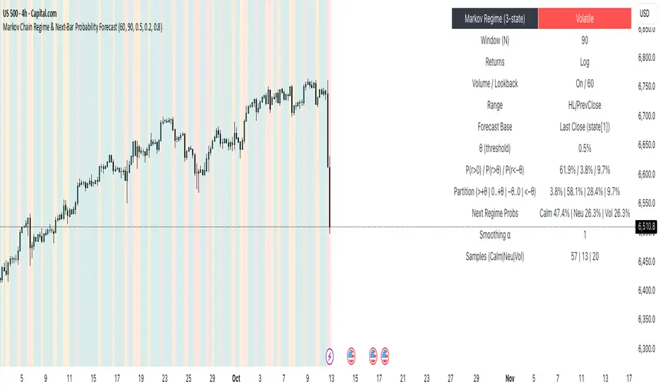
Markov Chain Regime & Next‑Bar Probability Forecast ✨ What it is A regime-aware, math-driven panel that forecasts the odds for the very next candle. It shows: • P(next r > 0) • P(next r > +θ) • P(next r < −θ) • A 4-bucket split of next-bar outcomes (>+θ | 0..+θ | −θ..0 | <−θ) • Next-regime probabilities: Calm | Neutral | Volatile 🧠 Why the math is strong • Markov regimes: Markets cluster in volatility “moods.” We learn a 3-state regime S∈{Calm, Neutral, Volatile} with a transition matrix A, where A = P(Sₜ₊₁=j | Sₜ=i). • Condition on the future state: We estimate event odds given the next regime j— q_pos(j)=P(rₜ₊₁>0 | Sₜ₊₁=j), q_gt(j)=P(rₜ₊₁>+θ | Sₜ₊₁=j), q_lt(j)=P(rₜ₊₁<−θ | Sₜ₊₁=j)— and mix them with transitions from the current (or frozen) state sNow: P(event) = Σⱼ A · q(event | j). This mixture-of-regimes view (HMM-style one-step prediction) ties next-bar outcomes to where volatility is likely headed. • Statistical hygiene: Laplace/Beta smoothing, minimum-sample gating, and unconditional fallbacks keep estimates stable. Heavy computations run on confirmed bars; “Freeze at close” avoids intrabar flicker. 📊 What each value means • Regime label & background: 🟩 Calm, 🟧 Neutral, 🟥 Volatile — quick read of market context. • P(next r > 0): Directional tilt for the very next bar. • P(next r > +θ): Odds of an outsized positive move beyond θ. • P(next r < −θ): Odds of an outsized negative move beyond −θ. • Partition row: Distributes next-bar probability across four intuitive buckets; they ≈ sum to 100%. • Next Regime Probs: Likelihood of switching to Calm/Neutral/Volatile on the next bar (row of A for the current/frozen state). • Samples row: How many next-bar samples support each next-state estimate (a confidence cue). • Smoothing α: The Laplace prior used to stabilize binary event rates. ⚙️ Inputs you control • Returns: Log (default) or % • Include Volume (z-score) + lookback • Include Range (HL/PrevClose) • Rolling window N (transitions & estimates) • θ as percent (e.g., 0.5%) • Freeze forecast at last close (recommended) • Display toggles (plots, partition, samples) 🎯 How to use it • Volatility awareness & sizing: Rising P(next regime = Volatile) → consider smaller size, wider stops, or skipping marginal entries. • Breakout preparation: Elevated P(next r > +θ) highlights environments where range expansion is more likely; pair with your setup/trigger. • Defense for mean-reversion: If P(next r < −θ) lifts while you’re late long (or P(next r > +θ) lifts while late short), tighten risk or wait for better context. • Calibration tip: Start θ near your market’s typical bar size; adjust until “>+θ” flags truly meaningful moves for your timeframe. 📝 Method notes & limits Activity features (|r|, volume z, range) are standardized; only positive z’s feed the composite activity score. Estimates adapt to instrument/timeframe; rare regimes or small windows increase variance (hence smoothing, sample gating, fallbacks). This is a context/forecast tool, not a standalone signal—combine with your entry/exit rules and risk management. 🧩 Strategies too We also develop full strategy versions that use these probabilities for entries, filters, and position sizing. Like this publication if you’d like us to release the strategy edition next. ⚠️ Disclaimer Educational use only. Not financial advice. Markets involve risk. Past performance does not guarantee future results.

Markov 3D Trend Analyzer Markov 3D Trend Analyzer 🔹 What Is a Markov State? A Markov chain models systems as states with probabilities of transitioning from one state to another. The key property is memorylessness: the next state depends only on the current state, not the full past history. In financial markets, this allows us to study how conditions tend to persist or flip — for example, whether a green candle is more likely to be followed by another green or by a red. 🔹 How This Indicator Uses It The Markov 3D Trend Analyzer tracks three independent Markov chains: Direction Chain (short-term): Probability that a green/red candle continues or reverses. Volatility Chain (mid-term): Probability of volatility staying Low/Medium/High or transitioning between them. Momentum Chain (structural): Probability of momentum (Bullish, Neutral, Bearish) persisting or flipping. Each chain is updated dynamically using exponentially weighted probabilities (EMA), which balance the law of large numbers (stability) with adaptivity to new market conditions. The indicator then classifies each chain’s dominant state and combines them into an actionable summary at the bottom of the table (e.g. “📈 Bullish breakout,” “⚠️ Choppy bearish fakeouts,” “⏳ Trend squeeze / possible reversal”). 🔹 Settings Direction Lookback / Volatility Lookback / Momentum Lookback Control the rolling window length (sample size) for each chain. Larger = smoother but slower to adapt. EMA Weight Adjusts how much weight is given to recent transitions vs. older history. Lower values adapt faster, higher values stabilize. Table Position Choose where the table is displayed on your chart. Table Size Adjust the font size for readability. 🔹 How To Consider Using Contextual tool: Use the summary row to understand the current market condition (trending, mean-reverting, expanding, compressing, continuation, fakeout risk). Complementary filter: Combine with your existing strategies to confirm or filter signals. For example: 📈 If your breakout strategy fires and the summary says Bullish breakout, that’s confirmation. ⚠️ If it says Choppy fakeouts, be cautious of traps. Visualization aid: The table lets you see how probabilities shift across direction, volatility, and momentum simultaneously. ⚠️ This indicator is not a signal generator. It is designed to help interpret market states probabilistically. Always use in conjunction with broader analysis and risk management. 🔹 Disclaimer This script is for educational and informational purposes only. It does not constitute financial advice or a recommendation to buy or sell any security, cryptocurrency, or instrument. Trading involves risk, and past probabilities or behaviors do not guarantee future outcomes. Always conduct your own research and use proper risk management.

Markov Chain Trend Probability A Markov Chain is a mathematical model that predicts future states based on the current state, assuming that the future depends only on the present (not the past). Originally developed by Russian mathematician Andrey Markov, this concept is widely used in: Finance: Risk modeling, portfolio optimization, credit scoring, algorithmic trading Weather Forecasting: Predicting sunny/rainy days, temperature patterns, storm tracking Here's an example of a Markov chain: If the weather is sunny, the probability that will be sunny 30 min later is say 90%. However, if the state changes, i.e. it starts raining, how the probability that will be raining 30 min later is say 70% and only 30% sunny. Similar concept can be applied to markets price action and trends. Mathematical Foundation The core principle follows the Markov Property: P(X_{t+1}|X_t, X_{t-1}, ..., X_0) = P(X_{t+1}|X_t) Transition Matrix : -------------Next State Current---- --------P11 P12 -----P21 P22 Probability Calculations: P(Up→Up) = Count(Up→Up) / Count(Up states) P(Down→Down) = Count(Down→Down) / Count(Down states) Steady-state probability: π = πP (where π is the stationary distribution) State Definition: State = UPTREND if (Price_t - Price_{t-n})/ATR > threshold State = DOWNTREND if (Price_t - Price_{t-n})/ATR < -threshold How It Works in Trading This indicator applies Markov Chain theory to market trends by: Defining States: Classifies market conditions as UPTREND or DOWNTREND based on price movement relative to ATR (Average True Range) Learning Transitions: Analyzes historical data to calculate probabilities of moving from one state to another Predicting Probabilities: Estimates the likelihood of future trend continuation or reversal How to Use Parameters: Lookback Period: Number of bars to analyze for trend detection (default: 14) ATR Threshold: Sensitivity multiplier for state changes (default: 0.5) Historical Periods: Sample size for probability calculations (default: 33) Trading Applications: Trend confirmation for entry/exit decisions Risk assessment through probability analysis Market regime identification Early warning system for potential trend reversals The indicator works on any timeframe and asset class. Enjoy!

[SGM Markov Chain]Introduction A Markov chain is a mathematical model that describes a system evolving over time among a finite number of states. This model is based on the assumption that the future state of the system depends only on the current state and not on previous states, the so-called Markov property. In the context of financial markets, Markov chains can be used to model transitions between different market conditions, for example, the probability of a price going up after going up, or going down after going down. Script Description This script uses a Markov chain to calculate closing price transition probabilities across the entire accessible chart. It displays the probabilities of the following transitions: - Up after Up (HH): Probability that the price rises after going up. - Down after Down (BB): Probability that the price will go down after going down. - Up after Down (HB): Probability that the price goes up after going down. - Down after Up (BH): Probability that the price will go down after going up. Features - Color customization: Choose colors for each transition type. - Table Position: Select the position of the probability display table (top/left, top/right, bottom/left, bottom/right).

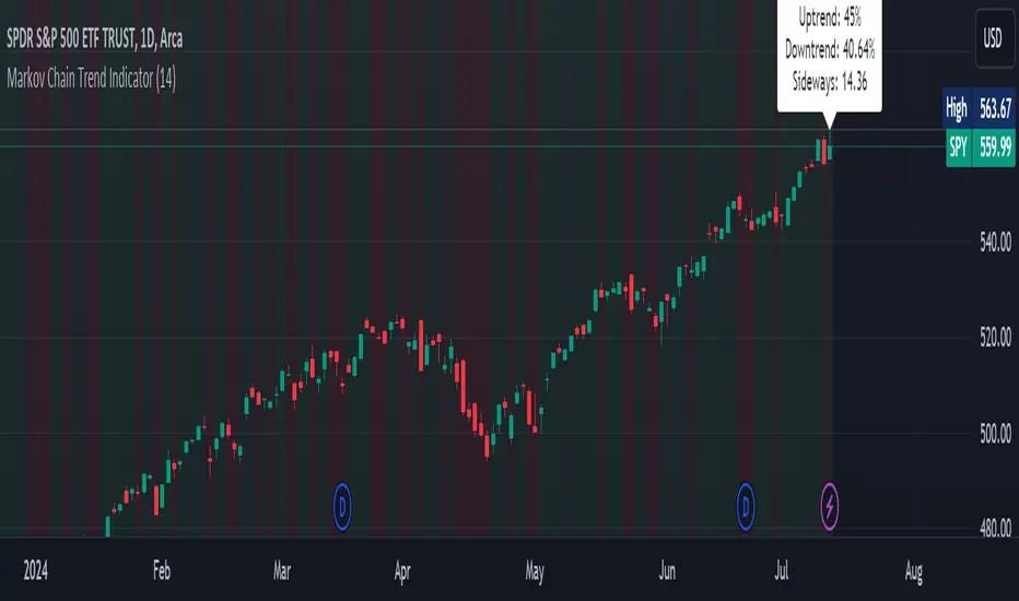
Markov Chain Trend Indicator Overview The Markov Chain Trend Indicator utilizes the principles of Markov Chain processes to analyze stock price movements and predict future trends. By calculating the probabilities of transitioning between different market states (Uptrend, Downtrend, and Sideways), this indicator provides traders with valuable insights into market dynamics. Key Features State Identification: Differentiates between Uptrend, Downtrend, and Sideways states based on price movements. Transition Probability Calculation: Calculates the probability of transitioning from one state to another using historical data. Real-time Dashboard: Displays the probabilities of each state on the chart, helping traders make informed decisions. Background Color Coding: Visually represents the current market state with background colors for easy interpretation. Concepts Underlying the Calculations Markov Chains: A stochastic process where the probability of moving to the next state depends only on the current state, not on the sequence of events that preceded it. Logarithmic Returns: Used to normalize price changes and identify states based on significant movements. Transition Matrices: Utilized to store and calculate the probabilities of moving from one state to another. How It Works The indicator first calculates the logarithmic returns of the stock price to identify significant movements. Based on these returns, it determines the current state (Uptrend, Downtrend, or Sideways). It then updates the transition matrices to keep track of how often the price moves from one state to another. Using these matrices, the indicator calculates the probabilities of transitioning to each state and displays this information on the chart. How Traders Can Use It Traders can use the Markov Chain Trend Indicator to: Identify Market Trends: Quickly determine if the market is in an uptrend, downtrend, or sideways state. Predict Future Movements: Use the transition probabilities to forecast potential market movements and make informed trading decisions. Enhance Trading Strategies: Combine with other technical indicators to refine entry and exit points based on predicted trends. Example Usage Instructions Add the Markov Chain Trend Indicator to your TradingView chart. Observe the background color to quickly identify the current market state: Green for Uptrend, Red for Downtrend, Gray for Sideways Check the dashboard label to see the probabilities of transitioning to each state. Use these probabilities to anticipate market movements and adjust your trading strategy accordingly. Combine the indicator with other technical analysis tools for more robust decision-making.

Function - simple* Markov Chain Monte Carlo Simulation (MCMC)Example function of a markov chain monte carlo simulation.