Volatility Formula - Instrument will move or notImpending Stock movement indicator. Blue and above 0, instrument will move. Orange no huge move expected.
Search in scripts for "Volatility"
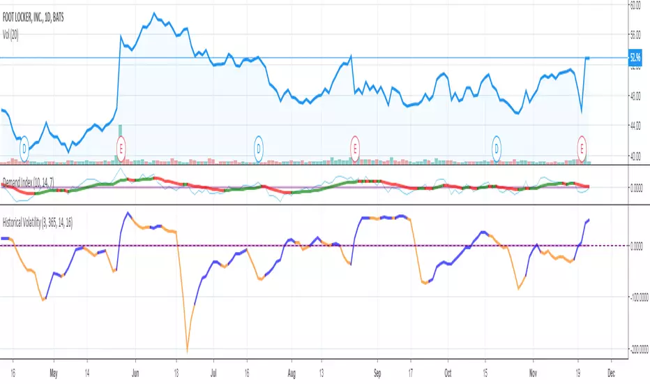
DROPTIONS_FIRED MTFVOLATILITY IN MULTITIMEFRAME. SHOOTING DOWNWARDS MEANING A MAJOR MOVEMENT HAS STARTED


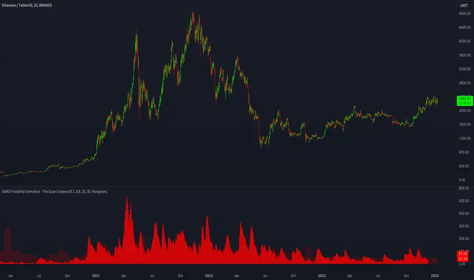
GARCH Volatility Estimation - The Quant ScienceThe GARCH (Generalized Autoregressive Conditional Heteroskedasticity) model is a statistical model used to forecast the volatility of a financial asset. This model takes into account the fluctuations in volatility over time, recognizing that volatility can vary in a heteroskedastic (i.e., non-constant variance) manner and can be influenced by past events.
The general formula of the GARCH model is:
σ²(t) = ω + α * ε²(t-1) + β * σ²(t-1)
where:
σ²(t) is the conditional variance at time t (i.e., squared volatility)
ω is the constant term (intercept) representing the baseline level of volatility
α is the coefficient representing the impact of the squared lagged error term on the conditional variance
ε²(t-1) is the squared lagged error term at the previous time period
β is the coefficient representing the impact of the lagged conditional variance on the current conditional variance
In the context of financial forecasting, the GARCH model is used to estimate the future volatility of the asset.
HOW TO USE
This quantitative indicator is capable of estimating the probable future movements of volatility. When the GARCH increases in value, it means that the volatility of the asset will likely increase as well, and vice versa. The indicator displays the relationship of the GARCH (bright red) with the trend of historical volatility (dark red).
USER INTERFACE
Alpha: select the starting value of Alpha (default value is 0.10).
Beta: select the starting value of Beta (default value is 0.80).
Lenght: select the period for calculating values within the model such as EMA (Exponential Moving Average) and Historical Volatility (default set to 20).
Forecasting: select the forecasting period, the number of bars you want to visualize data ahead (default set to 30).
Design: customize the indicator with your preferred color and choose from different types of charts, managing the design settings.
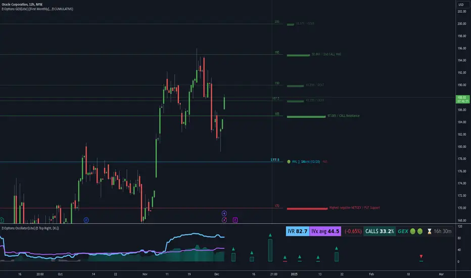
Options Oscillator [Lite] IVRank, IVx, Call/Put Volatility Skew The first TradingView indicator that provides REAL IVRank, IVx, and CALL/PUT skew data based on REAL option chain for 5 U.S. market symbols.
🔃 Auto-Updating Option Metrics without refresh!
🍒 Developed and maintained by option traders for option traders.
📈 Specifically designed for TradingView users who trade options.
🔶 Ticker Information:
This 'Lite' indicator is currently only available for 5 liquid U.S. market smbols : NASDAQ:TSLA AMEX:DIA NASDAQ:AAPL NASDAQ:AMZN and NYSE:ORCL
🔶 How does the indicator work and why is it unique?
This Pine Script indicator is a complex tool designed to provide various option metrics and visualization tools for options market traders. The indicator extracts raw options data from an external data provider (ORATS), processes and refines the delayed data package using pineseed, and sends it to TradingView, visualizing the data using specific formulas (see detailed below) or interpolated values (e.g., delta distances). This method of incorporating options data into a visualization framework is unique and entirely innovative on TradingView.
The indicator aims to offer a comprehensive view of the current state of options for the implemented instruments, including implied volatility (IV), IV rank (IVR), options skew, and expected market movements, which are objectively measured as detailed below.
The options metrics we display may be familiar to options traders from various major brokerage platforms such as TastyTrade, IBKR, TOS, Tradier, TD Ameritrade, Schwab, etc.
🟨 The following data is displayed in the oscillator 🟨
We use Tastytrade formulas, so our numbers mostly align with theirs!
🔶 𝗜𝗩𝗥𝗮𝗻𝗸
The Implied Volatility Rank (IVR) helps options traders assess the current level of implied volatility (IV) in comparison to the past 52 weeks. IVR is a useful metric to determine whether options are relatively cheap or expensive. This can guide traders on whether to buy or sell options.
IV Rank formula = (current IV - 52 week IV low) / (52 week IV high - 52 week IV low)
IVRank is default blue and you can adjust their settings:
🔶 𝗜𝗩𝘅 𝗮𝘃𝗴
The implied volatility (IVx) shown in the option chain is calculated like the VIX. The Cboe uses standard and weekly SPX options to measure expected S&P 500 volatility. A similar method is used for calculating IVx for each expiration cycle.
We aggregate the IVx values for the 35-70 day monthly expiration cycle, and use that value in the oscillator and info panel.
We always display which expiration the IVx values are averaged for when you hover over the IVx cell.
IVx main color is purple, but you can change the settings:
🔹IVx 5 days change %
We are also displaying the five-day change of the IV Index (IVx value). The IV Index 5-Day Change column provides quick insight into recent expansions or decreases in implied volatility over the last five trading days.
Traders who expect the value of options to decrease might view a decrease in IVX as a positive signal. Strategies such as Strangle and Ratio Spread can benefit from this decrease.
On the other hand, traders anticipating further increases in IVX will focus on the rising IVX values. Strategies like Calendar Spread or Diagonal Spread can take advantage of increasing implied volatility.
This indicator helps traders quickly assess changes in implied volatility, enabling them to make informed decisions based on their trading strategies and market expectations.
Important Note:
The IVx value alone does not provide sufficient context. There are stocks that inherently exhibit high IVx values. Therefore, it is crucial to consider IVx in conjunction with the Implied Volatility Rank (IVR), which measures the IVx relative to its own historical values. This combined view helps in accurately assessing the significance of the IVx in relation to the specific stock's typical volatility behavior.
This indicator offers traders a comprehensive view of implied volatility, assisting them in making informed decisions by highlighting both the absolute and relative volatility measures.
🔶 𝗖𝗔𝗟𝗟/𝗣𝗨𝗧 𝗣𝗿𝗶𝗰𝗶𝗻𝗴 𝗦𝗸𝗲𝘄 𝗵𝗶𝘀𝘁𝗼𝗴𝗿𝗮𝗺
At TanukiTrade, Vertical Pricing Skew refers to the difference in pricing between put and call options with the same expiration date at the same distance (at tastytrade binary expected move). We analyze this skew to understand market sentiment. This is the same formula used by TastyTrade for calculations.
We calculate the interpolated strike price based on the expected move, taking into account the neighboring option prices and their distances. This allows us to accurately determine whether the CALL or PUT options are more expensive.
🔹 What Causes Pricing Skew? The Theory Behind It
The asymmetric pricing of PUT and CALL options is driven by the natural dynamics of the market. The theory is that when CALL options are more expensive than PUT options at the same distance from the current spot price, market participants are buying CALLs and selling PUTs, expecting a faster upward movement compared to a downward one .
In the case of PUT skew, it's the opposite: participants are buying PUTs and selling CALLs , as they expect a potential downward move to happen more quickly than an upward one.
An options trader can take advantage of this phenomenon by leveraging PUT pricing skew. For example, if they have a bullish outlook and both IVR and IVx are high and IV started decreasing, they can capitalize on this PUT skew with strategies like a jade lizard, broken wing butterfly, or short put.
🔴 PUT Skew 🔴
Put options are more expensive than call options, indicating the market expects a faster downward move (▽). This alone doesn't indicate which way the market will move (because nobody knows that), but the options chain pricing suggests that if the market moves downward, it could do so faster in velocity compared to a potential upward movement.
🔹 SPY PUT SKEW example:
If AMEX:SPY PUT option prices are 46% higher than CALLs at the same distance for the optimal next monthly expiry (DTE). This alone doesn't indicate which way the market will move (because nobody knows that), but the options chain pricing suggests that if the market moves downward, it could do so 46% faster in velocity compared to a potential upward movement
🟢 CALL Skew 🟢
Call options are more expensive than put options, indicating the market expects a faster upward move (△). This alone doesn't indicate which way the market will move (because nobody knows that), but the options chain pricing suggests that if the market moves upward, it could do so faster in velocity compared to a potential downward movement.
🔹 INTC CALL SKEW example:
If NASDAQ:INTC CALL option prices are 49% higher than PUTs at the same distance for the optimal next monthly expiry (DTE). This alone doesn't indicate which way the market will move (because nobody knows that), but the options chain pricing suggests that if the market moves upward, it could do so 49% faster in velocity compared to a potential downward movement .
🔶 USAGE example:
The script is compatible with our other options indicators.
For example: Since the main metrics are already available in this Options Oscillator, you can hide the main IVR panel of our Options Overlay indicator, freeing up more space on the chart. The following image shows this:
🔶 ADDITIONAL IMPORTANT COMMENTS
🔹 Historical Data:
Yes, we only using historical internal metrics dating back to 2024-07-01, when the TanukiTrade options brand launched. For now, we're using these, but we may expand the historical data in the future.
🔹 What distance does the indicator use to measure the call/put pricing skew?:
It is important to highlight that this oscillator displays the call/put pricing skew changes for the next optimal monthly expiration on a histogram.
The Binary Expected Move distance is calculated using the TastyTrade method for the next optimal monthly expiration: Formula = (ATM straddle price x 0.6) + (1st OTM strangle price x 0.3) + (2nd OTM strangle price x 0.1)
We interpolate the exact difference based on the neighboring strikes at the binary expected move distance using the TastyTrade method, and compare the interpolated call and put prices at this specific point.
🔹 - Why is there a slight difference between the displayed data and my live brokerage data?
There are two reasons for this, and one is beyond our control.
◎ Option-data update frequency:
According to TradingView's regulations and guidelines, we can update external data a maximum of 5 times per day. We strive to use these updates in the most optimal way:
(1st update) 15 minutes after U.S. market open
(2nd, 3rd, 4th updates) 1.5–3 hours during U.S. market open hours
(5th update) 10 minutes before U.S. market close.
You don’t need to refresh your window, our last refreshed data-pack is always automatically applied to your indicator, and you can see the time elapsed since the last update at the bottom of the corner on daily TF.
◎ Brokerage Calculation Differences:
Every brokerage has slight differences in how they calculate metrics like IV and IVx. If you open three windows for TOS, TastyTrade, and IBKR side by side, you will notice that the values are minimally different. We had to choose a standard, so we use the formulas and mathematical models described by TastyTrade when analyzing the options chain and drawing conclusions.
🔹 - EOD data:
The indicator always displays end-of-day (EOD) data for IVR, IV, and CALL/PUT pricing skew. During trading hours, it shows the current values for the ongoing day with each update, and at market close, these values become final. From that point on, the data is considered EOD, provided the day confirms as a closed daily candle.
🔹 - U.S. market only:
Since we only deal with liquid option chains: this option indicator only works for the USA options market and do not include future contracts; we have implemented each selected symbol individually.
Disclaimer:
Our option indicator uses approximately 15min-3 hour delayed option market snapshot data to calculate the main option metrics. Exact realtime option contract prices are never displayed; only derived metrics and interpolated delta are shown to ensure accurate and consistent visualization. Due to the above, this indicator can only be used for decision support; exclusive decisions cannot be made based on this indicator. We reserve the right to make errors.This indicator is designed for options traders who understand what they are doing. It assumes that they are familiar with options and can make well-informed, independent decisions. We work with public data and are not a data provider; therefore, we do not bear any financial or other liability.
VIX Volatility Trend Analysis With Signals - Stocks OnlyVIX VOLATILITY TREND ANALYSIS CLOUD WITH BULLISH & BEARISH SIGNALS - STOCKS ONLY
This indicator is a visual aid that shows you the bullish or bearish trend of VIX market volatility so you can see the VIX trend without switching charts. When volatility goes up, most stocks go down and vice versa. When the cloud turns green, it is a bullish sign. When the cloud turns red, it is a bearish sign.
This indicator is meant for stocks with a lot of price action and volatility, so for best results, use it on charts that move similar to the S&P 500 or other similar charts.
This indicator uses real time data from the stock market overall, so it should only be used on stocks and will only give a few signals during after hours. It does work ok for crypto, but will not give signals when the US stock market is closed.
**HOW TO USE**
When the VIX Volatility Index trend changes direction, it will give a green or red line on the chart depending on which way the VIX is now trending. The cloud will also change color depending on which way the VIX is trending. Use this to determine overall market volatility and place trades in the direction that the indicator is showing. Do not use this by itself as sometimes markets won’t react perfectly to the overall market volatility. It should only be used as a secondary confirmation in your trading/trend analysis.
For more signals with earlier entries, go into settings and reduce the number. 10-100 is best for scalping. For less signals with later entries, change the number to a higher value. Use 100-500 for swing trades. Can go higher for long swing trades. Our favorite settings are 20, 60, 100, 500 and 1000.
***MARKETS***
This indicator should only be used on the US stock markets as signals are given based on the VIX volatility index which measures volatility of the US Stock Markets.
***TIMEFRAMES***
This indicator works on all time frames, but after hours will not change much at all due to the markets being closed.
**INVERSE CHARTS**
If you are using this on an inverse ETF and the signals are showing backwards, please comment with what chart it is and I will configure the indicator to give the correct signals. I have included over 50 inverse ETFs into the code to show the correct signals on inverse charts, but I'm sure there are some that I have missed so feel free to let me know and I will update the script with the requested tickers.
***TIPS***
Try using numerous indicators of ours on your chart so you can instantly see the bullish or bearish trend of multiple indicators in real time without having to analyze the data. Some of our favorites are our Auto Fibonacci, Directional Movement Index, Volume Profile with buy & sell pressure, Auto Support And Resistance, Vix Scalper and Money Flow Index in combination with this Vix Trend Analysis. They all have real time Bullish and Bearish labels as well so you can immediately understand each indicator's trend.

Rainbow EMA Areas with Volatility HighlightThe indicator provides traders with an enhanced visual tool to observe price movements, trend strength, and market volatility on their charts. It combines multiple EMAs (Exponential Moving Averages) with color-coded areas to indicate the market’s directional bias and a high-volatility highlight for detecting times of increased market activity.
Explanation of Key Components
Multiple EMAs (Exponential Moving Averages):
Six different EMAs are calculated for various periods (15, 45, 100, 150, 200, 300).
Each EMA period represents a different timeframe, from short-term to long-term trends, providing a well-rounded view of price behavior across different market cycles.
The EMAs are color-coded for easy differentiation:
Green shades indicate bullish trends when prices are above the EMAs.
Red shades indicate bearish trends when prices are below the EMAs.
The space between each EMA is filled with a gradient color, creating a "wave" effect that helps identify the market’s overall direction.
ATR-Based Volatility Detection:
The ATR (Average True Range), a measure of market volatility, is used to assess how much the price is fluctuating. When volatility is high, price movements are typically more significant, indicating potential trading opportunities or times to exercise caution.
The indicator calculates ATR and uses a customizable multiplier to set a high-volatility threshold.
When the ATR exceeds this threshold, it signals that the market is experiencing high volatility.
Visual High Volatility Highlight:
A yellow background appears on the chart during periods of high volatility, giving a subtle but clear visual indication that the market is active.
This highlight helps traders spot potential breakout areas or increased activity zones without obstructing the EMA areas.
Volatility Signal Markers:
Small, red triangular markers are plotted above price bars when high volatility is detected, marking these areas for additional emphasis.
These signals serve as alerts to help traders quickly recognize high volatility moments where price moves may be stronger.
How to Use This Indicator
Identify Trends Using EMA Areas:
Bullish Trend: When the price is above most or all EMAs, and the EMA areas are colored in shades of green, it indicates a strong bullish trend. Traders might look for buy opportunities in this scenario.
Bearish Trend: When the price is below most or all EMAs, and the EMA areas are colored in shades of red, it signals a bearish trend. This condition can suggest potential sell opportunities.
Consolidation or Neutral Trend: If the price is moving within the EMA bands without a clear green or red dominance, the market may be in a consolidation phase. This period often precedes a breakout in either direction.
Volatility-Based Entries and Exits:
High Volatility Areas: The yellow background and red triangular markers signal high-volatility areas. This information can be valuable for identifying potential breakout points or strong moves.
Trading in High Volatility: During high-volatility phases, the market may experience rapid price changes, which can be ideal for breakout trades. However, high volatility also involves higher risk, so traders may adjust their strategies accordingly (e.g., setting wider stops or adjusting position sizes).
Trading in Low Volatility: When the yellow background and markers are absent, volatility is lower, indicating a calmer market. In these times, traders may choose to look for range-bound trading opportunities or wait for the next trend to develop.
Combining with Other Indicators:
This indicator works well in combination with momentum or oscillating indicators like RSI or MACD, providing a well-rounded view of the market.
For example, if the indicator shows a bullish EMA area with high volatility, and an RSI is trending up, it could be a stronger buy signal. Conversely, if the indicator shows a bearish EMA area with high volatility and RSI is trending down, this could be a stronger sell signal.
Practical Trading Examples
Bullish Trend in High Volatility:
Price is above the EMAs, showing green EMA areas, and the high volatility background is active.
This indicates a strong bullish trend with significant price movement potential.
A trader could look for breakout or continuation entries in the direction of the trend.
Bearish Reversal Signal:
Price crosses below the EMAs, showing red EMA areas, while high volatility is also detected.
This suggests that the market may be reversing to a bearish trend with increased price movement.
Traders could consider taking short positions or setting stops on existing long trades.
This indicator is designed to provide a rich visual experience, making it easy to spot trends, consolidations, and volatility zones at a glance. It is best used by traders who benefit from visual cues and who seek a quick understanding of both trend direction and market activity. Let me know if you'd like further customization or additional functionalities!

Z-Score Based Momentum Zones with Advanced Volatility ChannelsThe indicator "Z-Score Based Momentum Zones with Advanced Volatility Channels" combines various technical analysis components, including volatility, price changes, and volume correction, to calculate Z-Scores and determine momentum zones and provide a visual representation of price movements and volatility based on multi timeframe highest high and lowest low values.
Note: THIS IS A IMPROVEMNT OF "Multi Time Frame Composite Bands" INDICATOR OF MINE WITH MORE EMPHASIS ON MOMENTUM ZONES CALULATED BASED ON Z-SCORES
Input Options
look_back_length: This input specifies the look-back period for calculating intraday volatility. correction It is set to a default value of 5.
lookback_period: This input sets the look-back period for calculating relative price change. The default value is 5.
zscore_period: This input determines the look-back period for calculating the Z-Score. The default value is 500.
avgZscore_length: This input defines the length of the momentum block used in calculations, with a default value of 14.
include_vc: This is a boolean input that, if set to true, enables volume correction in the calculations. By default, it is set to false.
1. Volatility Bands (Composite High and Low):
Composite High and Low: These are calculated by combining different moving averages of the high prices (high) and low prices (low). Specifically:
a_high and a_low are calculated as the average of the highest (ta.highest) and lowest (ta.lowest) high and low prices over various look-back periods (5, 8, 13, 21, 34) to capture short and long-term trends.
b_high and b_low are calculated as the simple moving average (SMA) of the high and low prices over different look-back periods (5, 8, 13) to smooth out the trends.
high_c and low_c are obtained by averaging a_high with b_high and a_low with b_low respectively.
IDV Correction Calulation : In this script the Intraday Volatility (IDV) is calculated as the simple moving average (SMA) of the daily high-low price range divided by the closing price. This measures how much the price fluctuates in a given period.
Composite High and Low with Volatility: The final c_high and c_low values are obtained by adjusting high_c and low_c with the calculated intraday volatility (IDV). These values are used to create the "Composite High" and "Composite Low" plots.
Composite High and Low with Volatility Correction: The final c_high and c_low values are obtained by adjusting high_c and low_c with the calculated intraday volatility (IDV). These values are used to create the "Composite High" and "Composite Low" plots.
2. Momentum Blocks Based on Z-Score:
Relative Price Change (RPC):
The Relative Price Change (rpdev) is calculated as the difference between the current high-low-close average (hlc3) and the previous simple moving average (psma_hlc3) of the same quantity. This measures the change in price over time.
Additionally, std_hlc3 is calculated as the standard deviation of the hlc3 values over a specified look-back period. The standard deviation quantifies the dispersion or volatility in the price data.
The rpdev is then divided by the std_hlc3 to normalize the price change by the volatility. This normalization ensures that the price change is expressed in terms of standard deviations, which is a common practice in quantitative analysis.
Essentially, the rpdev represents how many standard deviations the current price is away from the previous moving average.
Volume Correction (VC): If the include_vc input is set to true, volume correction is applied by dividing the trading volume by the previous simple moving average of the volume (psma_volume). This accounts for changes in trading activity.
Volume Corrected Relative Price Change (VCRPD): The vcrpd is calculated by multiplying the rpdev by the volume correction factor (vc). This incorporates both price changes and volume data.
Z-Scores: The Z-scores are calculated by taking the difference between the vcrpd and the mean (mean_vcrpd) and then dividing it by the standard deviation (stddev_vcrpd). Z-scores measure how many standard deviations a value is away from the mean. They help identify whether a value is unusually high or low compared to its historical distribution.
Momentum Blocks: The "Momentum Blocks" are essentially derived from the Z-scores (avgZScore). The script assigns different colors to the "Fill Area" based on predefined Z-score ranges. These colored areas represent different momentum zones:
Positive Z-scores indicate bullish momentum, and different shades of green are used to fill the area.
Negative Z-scores indicate bearish momentum, and different shades of red are used.
Z-scores near zero (between -0.25 and 0.25) suggest neutrality, and a yellow color is used.

Conditional Volatility Explosion/ContractionThis indicator identifies zones of potential volatility expansion by analyzing the contraction and expansion of volatility bands, which are conditioned by the relationship of the price to moving averages
Volatility Squeeze: When the bands contract, it indicates a potential buildup in market tension, often preceding a significant price movement.
Volatility Expansion: When the bands expand, it signals the release of built-up tension, often resulting in increased volatility.
Trend Confirmation: The bands are active only when the price aligns with the moving average condition, helping to filter out less relevant signals during non-trending markets.
Upper Band: Displays as a red band when the volatility condition is met.
Represents the upper boundary of potential price action during high volatility.
Lower Band: Displays as a green band when the volatility condition is met.
Represents the lower boundary of potential price action during high volatility.
Fill Areas: The areas between the EMA and the bands are filled with transparent colors:
Red for the upper fill.
Green for the lower fill.
These highlights help visualize zones of potential volatility explosion.

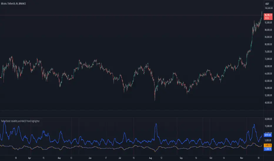
TechniTrend: Volatility and MACD Trend Highlighter🟦 Overview
The "Candle Volatility with Trend Prediction" indicator is a powerful tool designed to identify market volatility based on candle movement relative to average volume while also incorporating trend predictions using the MACD. This indicator is ideal for traders who want to detect volatile market conditions and anticipate potential price movements, leveraging both price changes and volume dynamics.
It not only highlights candles with significant price movements but also integrates a trend analysis based on the MACD (Moving Average Convergence Divergence), allowing traders to gauge whether the market momentum aligns with or diverges from the detected volatility.
🟦 Key Features
🔸Volatility Detection: Identifies candles that exceed normal price fluctuations based on average volume and recent price volatility.
🔸Trend Prediction: Uses the MACD indicator to overlay trend analysis, signaling potential market direction shifts.
🔸Volume-Based Analysis: Integrates customizable moving averages (SMA, EMA, WMA, etc.) of volume, providing a clear visualization of volume trends.
🔸Alert System: Automatically notifies traders of high-volatility situations, aiding in timely decision-making.
🔸Customizability: Includes multiple settings to tailor the indicator to different market conditions and timeframes.
🟦 How It Works
The indicator operates by evaluating the price volatility in relation to average volume and identifying when a candle's volatility surpasses a threshold defined by the user. The key calculations include:
🔸Average Volume Calculation: The user selects the type of moving average (SMA, EMA, etc.) to calculate the average volume over a set period.
🔸Volatility Measurement: The indicator measures the body change (difference between open and close) and the high-low range of each candle. It then calculates recent price volatility using a standard deviation over a user-defined length.
🔸Weighted Index: A unique index is created by dividing price change by average volume and recent volatility.
🔸Highlighting Volatility: If the weighted index exceeds a customizable threshold, the candle is highlighted, indicating potential trading opportunities.
🔸Trend Analysis with MACD: The MACD line and signal line are plotted and adjusted with a user-defined multiplier to visualize trends alongside the volatility signals.
🟦 Recommended Settings
🔸Volume MA Length: A default of 14 periods for the average volume calculation is recommended. Adjust to higher periods for long-term trends and shorter periods for quick trades.
🔸Volatility Threshold Multiplier: Set at 1.2 by default to capture moderately significant movements. Increase for fewer but stronger signals or decrease for more frequent signals.
🔸MACD Settings: Default MACD parameters (12, 26, 9) are suggested. Tweak based on your trading strategy and asset volatility.
🔸MACD Multiplier: Adjust based on how the MACD should visually compare to the average volume. A multiplier of 1 works well for most cases.
🟦 How to Use
🔸Volatile Market Detection:
Look for highlighted candles that suggest a deviation from typical price behavior. These candles often signify an entry point for short-term trades.
🔸Trend Confirmation:
Use the MACD trend analysis to verify if the highlighted volatile candles align with a bullish or bearish trend.
For example, a bullish MACD crossover combined with a highlighted candle suggests a potential uptrend, while a bearish crossover with volatility signals may indicate a downtrend.
🔸Volume-Driven Strategy:
Observe how volume changes impact candle volatility. When volume rises significantly and candles are highlighted, it can suggest strong market moves influenced by big players.
🟦 Best Use Cases
🔸Trend Reversals: Detect potential trend reversals early by spotting divergences between price and MACD within volatile conditions.
🔸Breakout Strategies: Use the indicator to confirm price breakouts with significant volume changes.
🔸Scalping or Day Trading: Customize the indicator for shorter timeframes to capture rapid market movements based on volatility spikes.
🔸Swing Trading: Combine volatility and trend insights to optimize entry and exit points over longer periods.
🟦 Customization Options
🔸Volume-Based Inputs: Choose from SMA, EMA, WMA, and more to define how average volume is calculated.
🔸Threshold Adjustments: Modify the volatility threshold multiplier to increase or decrease sensitivity based on your trading style.
🔸MACD Tuning: Adjust MACD settings and the multiplier for trend visualization tailored to different asset classes and market conditions.
🟦 Indicator Alerts
🔸High Volatility Alerts: Automatically triggered when candles exceed user-defined volatility levels.
🔸Bullish/Bearish Trend Alerts: Alerts are activated when highlighted volatile candles align with bullish or bearish MACD crossovers, making it easier to spot opportunities without constantly monitoring the chart.
🟦 Examples of Use
To better understand how this indicator works, consider the following scenarios:
🔸Example 1: In a strong uptrend, observe how volume surges and volatility highlight candles right before price consolidations, indicating optimal exit points.
🔸Example 2: During a downtrend, see how the MACD aligns with volume-driven volatility, signaling potential short-selling opportunities.
Conditional Volatility PercentileSimple Description: This indicator can basically help you find when a big move might happen ( This indicator can't determine the direction but when a big move could happen. ) Basically, a low-extreme value like 0 means that it only has room for upside, so volatility can only expand from that point on, and the fact that volatility mean reverts supports this.
Conditional Volatility Percentile Indicator
This indicator is a tool designed to view current market volatility relative to historical levels. It uses a statistical approach to assess the percentile rank of the calculated conditional volatility.
The Volatility Calculation
This indicator calculates conditional variance with user-defined parameters, which are Omega, Alpha, Beta, and Sigma, and then takes the square root of the variance to calculate the standard deviation. The script then calculates the percentile rank of the conditional variance over a specified lookback.
What this indicator tells you:
Volatility Assessment: Higher percentile values indicate heightened conditional volatility, suggesting increased market activity or potential stress. Meanwhile, lower percentiles suggest relatively lower conditional volatility.
Extreme Values: Volatility is a mean-reverting process. If the volatility percentile value is at a low value for an extended period of time, you can eventually bet on the volatility percentile value increasing with high confidence.
In financial markets, volatility itself exhibits mean-reverting properties. This means that periods of high volatility are likely to be followed by periods of lower volatility, and vice versa.
1. High Volatility Periods: High volatility levels may be followed by a subsequent decrease in volatility as the market returns to a more typical state.
2. Low Volatility Periods: Periods of low volatility may be followed by an uptick in volatility as the market experiences new information or changes in sentiment.
SOLANA Performance & Volatility Analysis BB%Overview:
The script provides an in-depth analysis of Solana's performance and volatility. It showcases Solana's price, its inverse relationship, its own volatility, and even juxtaposes it against Bitcoin's 24-hour historical volatility. All of these are presented using the Bollinger Bands Percentage (BB%) methodology to normalise the price and volatility values between 0 and 1.
Key Components:
Inputs:
SOLANA PRICE (SOLUSD): The price of Solana.
SOLANA INVERSE (SOLUSDT.3S): The inverse of Solana's price.
SOLANA VOLATILITY (SOLUSDSHORTS): Volatility for Solana.
BITCOIN 24 HOUR HISTORICAL VOLATILITY (BVOL24H): Bitcoin's volatility over the past 24 hours.
BB Calculations:
The script uses the Bollinger Bands methodology to calculate the mean (SMA) and the standard deviation of the prices and volatilities over a certain period (default is 20 periods). The calculated upper and lower bands help in normalising the values to the range of 0 to 1.
Normalised Metrics Plotting:
For better visualisation and comparative analysis, the normalised values for:
Solana Price
Solana Inverse
Solana Volatility
Bitcoin 24hr Volatility
are plotted with steplines.
Band Plotting:
Bands are plotted at 20%, 40%, 60%, and 80% levels to serve as reference points. The area between the 40% and 60% bands is shaded to highlight the median region.
Colour Coding:
Different colours are used for easy differentiation:
Solana Price: Blue
Solana Inverse: Red
Solana Volatility: Green
Bitcoin 24hr Volatility: White
Licence & Creator:
The script adheres to the Mozilla Public Licence 2.0 and is credited to the author, "Volatility_Vibes".
Works well with Breaks and Retests with Volatility Stop

Bandwidth Volatility - Silverman Rule of thumb EstimatorOverview
This indicator calculates volatility using the Rule of Thumb bandwidth estimator and incorporating the standard deviations of returns to get historical volatility. There are two options: one for the original rule of thumb bandwidth estimator, and another for the modified rule of thumb estimator. This indicator comes with the bandwidth , which is shown with the color gradient columns, which are colored by a percentile of the bandwidth, and the moving average of the bandwidth, which is the dark shaded area.
The rule of thumb bandwidth estimator is a simple and quick method for estimating the bandwidth parameter in kernel density estimation (KSE) or kernel regression. It provides a rough approximation of the bandwidth without requiring extensive computation resources or fine-tuning. One common rule of thumb estimator is Silverman rule, which is given by
h = 1.06*σ*n^(-1/5)
where
h is the bandwidth
σ is the standard deviation of the data
n is the number of data points
This rule of thumb is based on assuming a Gaussian kernel and aims to strike a balance between over-smoothing and under-smoothing the data. It is simple to implement and usually provides reasonable bandwidth estimates for a wide range of datasets. However , it is important to note that this rule of thumb may not always have optimal results, especially for non-Gaussian or multimodal distributions. In such cases, a modified bandwidth selection, such as cross-validation or even applying a log transformation (if the data is right-skewed), may be preferable.
How it works:
This indicator computes the bandwidth volatility using returns, which are used in the standard deviation calculation. It then estimates the bandwidth based on either the Silverman rule of thumb or a modified version considering the interquartile range. The percentile ranks of the bandwidth estimate are then used to visualize the volatility levels, identify high and low volatility periods, and show them with colors.
Modified Rule of thumb Bandwidth:
The modified rule of thumb bandwidth formula combines elements of standard deviations and interquartile ranges, scaled by a multiplier of 0.9 and inversely with a number of periods. This modification aims to provide a more robust and adaptable bandwidth estimation method, particularly suitable for financial time series data with potentially skewed or heavy-tailed data.
Formula for Modified Rule of Thumb Bandwidth:
h = 0.9 * min(σ, (IQR/1.34))*n^(-1/5)
This modification introduces the use of the IQR divided by 1.34 as an alternative to the standard deviation. It aims to improve the estimation, mainly when the underlying distribution deviates from a perfect Gaussian distribution.
Analysis
Rule of thumb Bandwidth: Provides a broader perspective on volatility trends, smoothing out short-term fluctuations and focusing more on the overall shape of the density function.
Historical Volatility: Offers a more granular view of volatility, capturing day-to-day or intra-period fluctuations in asset prices and returns.
Modelling Requirements
Rule of thumb Bandwidth: Provides a broader perspective on volatility trends, smoothing out short-term fluctuations and focusing more on the overall shape of the density function.
Historical Volatility: Offers a more granular view of volatility, capturing day-to-day or intra-period fluctuations in asset prices and returns.
Pros of Bandwidth as a volatility measure
Robust to Data Distribution: Bandwidth volatility, especially when estimated using robust methods like Silverman's rule of thumb or its modifications, can be less sensitive to outliers and non-normal distributions compared to some other measures of volatility
Flexibility: It can be applied to a wide range of data types and can adapt to different underlying data distributions, making it versatile for various analytical tasks.
How can traders use this indicator?
In finance, volatility is thought to be a mean-reverting process. So when volatility is at an extreme low, it is expected that a volatility expansion happens, which comes with bigger movements in price, and when volatility is at an extreme high, it is expected for volatility to eventually decrease, leading to smaller price moves, and many traders view this as an area to take profit in.
In the context of this indicator, low volatility is thought of as having the green color, which indicates a low percentile value, and also being below the moving average. High volatility is thought of as having the yellow color and possibly being above the moving average, showing that you can eventually expect volatility to decrease.

Grid by Volatility (Expo)█ Overview
The Grid by Volatility is designed to provide a dynamic grid overlay on your price chart. This grid is calculated based on the volatility and adjusts in real-time as market conditions change. The indicator uses Standard Deviation to determine volatility and is useful for traders looking to understand price volatility patterns, determine potential support and resistance levels, or validate other trading signals.
█ How It Works
The indicator initiates its computations by assessing the market volatility through an established statistical model: the Standard Deviation. Following the volatility determination, the algorithm calculates a central equilibrium line—commonly referred to as the "mid-line"—on the chart to serve as a baseline for additional computations. Subsequently, upper and lower grid lines are algorithmically generated and plotted equidistantly from the central mid-line, with the distance being dictated by the previously calculated volatility metrics.
█ How to Use
Trend Analysis: The grid can be used to analyze the underlying trend of the asset. For example, if the price is above the Average Line and moves toward the Upper Range, it indicates a strong bullish trend.
Support and Resistance: The grid lines can act as dynamic support and resistance levels. Price tends to bounce off these levels or breakthrough, providing potential trade opportunities.
Volatility Gauge: The distance between the grid lines serves as a measure of market volatility. Wider lines indicate higher volatility, while narrower lines suggest low volatility.
█ Settings
Volatility Length: Number of bars to calculate the Standard Deviation (Default: 200)
Squeeze Adjustment: Multiplier for the Standard Deviation (Default: 6)
Grid Confirmation Length: Number of bars to calculate the weighted moving average for smoothing the grid lines (Default: 2)
-----------------
Disclaimer
The information contained in my Scripts/Indicators/Ideas/Algos/Systems does not constitute financial advice or a solicitation to buy or sell any securities of any type. I will not accept liability for any loss or damage, including without limitation any loss of profit, which may arise directly or indirectly from the use of or reliance on such information.
All investments involve risk, and the past performance of a security, industry, sector, market, financial product, trading strategy, backtest, or individual's trading does not guarantee future results or returns. Investors are fully responsible for any investment decisions they make. Such decisions should be based solely on an evaluation of their financial circumstances, investment objectives, risk tolerance, and liquidity needs.
My Scripts/Indicators/Ideas/Algos/Systems are only for educational purposes!

MAD Volatility PercentileMean Absolute Deviation (MAD) is a statistical measure that tells you how spread out or variable a set of data points is. It calculates the average distance of each data point from the mean (average) of the data set. MAD helps you understand how much individual values differ from the average value. It's a way to measure the overall "average distance" of the data points from the center point.
Indicator Overview:
This indicator measures market volatility using Mean Absolute Deviation of returns. The MAD Volatility Percentile Indicator calculates and represents market volatility as a percentile. The lower the percentile, the lower the volatility, and the higher the percentile value is, the higher the volatility is.
Understanding Volatility:
Lower percentiles signify a lower volatility market environment, reflecting reduced volatility, while higher percentiles indicate increased volatility and significant price movements. The indicator also comes with an SMA to see when the burst of higher volatility occur. You can also change the sample length on the indicators option. You can consider a big move occurring when the percentile value is above the SMA.
Application
Generally when the Mean Absolute Deviation Volatility Percentile is low, then this means that the volatility is low and a expansion could happen soon, which means a big move will occur soon. This indicator can also protect you from entering a trade that will not have any significant moves for a while.
This indicator is not a directional indicator but it can be applied with directional indicators, and is extremely versatile. For example you can use it with momentum indicators and if there is low volatility and bullish momentum then this can be a signal to potentially place a long position.
Features:
The percentile length sets the lookback of the percentile which calculates the percentile of the Mean Absolute Deviation of returns.
Sample length: Gets the volatility sample (returns)
SMA Length: The SMA of the percentile. Used to find when a move can be considered as an "expansion"
Alerts: You can also enable color alerts that flash when the volatility is at extremely low levels which can signify that a big move could happen soon.
This is an example of the alerts that the indicator comes with.

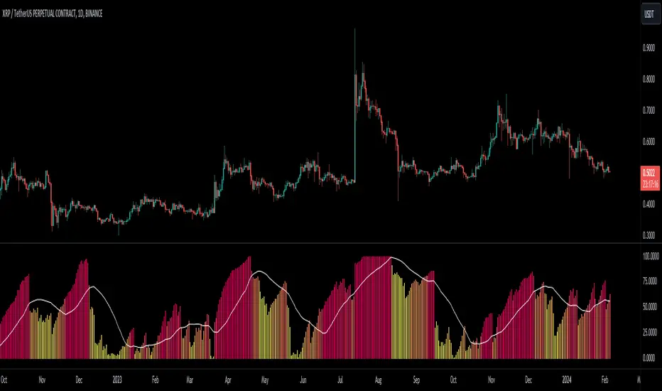
Relative Volatility Mass [SciQua]The ⚖️ Relative Volatility Mass (RVM) is a volatility-based tool inspired by the Relative Volatility Index (RVI) .
While the RVI measures the ratio of upward to downward volatility over a period, RVM takes a different approach:
It sums the standard deviation of price changes over a rolling window, separating upward volatility from downward volatility .
The result is a measure of the total “volatility mass” over a user-defined period, rather than an average or normalized ratio.
This makes RVM particularly useful for identifying sustained high-volatility conditions without being diluted by averaging.
────────────────────────────────────────────────────────────
╭────────────╮
How It Works
╰────────────╯
1. Standard Deviation Calculation
• Computes the standard deviation of the chosen `Source` over a `Standard Deviation Length` (`stdDevLen`).
2. Directional Separation
• Volatility on up bars (`chg > 0`) is treated as upward volatility .
• Volatility on down bars (`chg < 0`) is treated as downward volatility .
3. Rolling Sum
• Over a `Sum Length` (`sumLen`), the upward and downward volatilities are summed separately using `math.sum()`.
4. Relative Volatility Mass
• The two sums are added together to get the total volatility mass for the rolling window.
Formula:
RVM = Σ(σ up) + Σ(σ down)
where σ is the standard deviation over `stdDevLen`.
╭────────────╮
Key Features
╰────────────╯
Directional Volatility Tracking – Differentiates between volatility during price advances vs. declines.
Rolling Volatility Mass – Shows the total standard deviation accumulation over a given period.
Optional Smoothing – Multiple MA types, including SMA, EMA, SMMA (RMA), WMA, VWMA.
Bollinger Band Overlay – Available when SMA is selected, with adjustable standard deviation multiplier.
Configurable Source – Apply RVM to `close`, `open`, `hl2`, or any custom source.
╭─────╮
Usage
╰─────╯
Trend Confirmation: High RVM values can confirm strong trending conditions.
Breakout Detection: Spikes in RVM often precede or accompany price breakouts.
Volatility Cycle Analysis: Compare periods of contraction and expansion.
RVM is not bounded like the RVI, so absolute values depend on market volatility and chosen parameters.
Consider normalizing or using smoothing for easier visual comparison.
╭────────────────╮
Example Settings
╰────────────────╯
Short-term volatility detection: `stdDevLen = 5`, `sumLen = 10`
Medium-term trend volatility: `stdDevLen = 14`, `sumLen = 20`
Enable `SMA + Bollinger Bands` to visualize when volatility is unusually high or low relative to recent history.
╭───────────────────╮
Notes & Limitations
╰───────────────────╯
Not a directional signal by itself — use alongside price structure, volume, or other indicators.
Higher `sumLen` will smooth short-term fluctuations but reduce responsiveness.
Because it sums, not averages, values will scale with both volatility and chosen window size.
╭───────╮
Credits
╰───────╯
Based on the Relative Volatility Index concept by Donald Dorsey (1993).
TradingView
SciQua - Joshua Danford
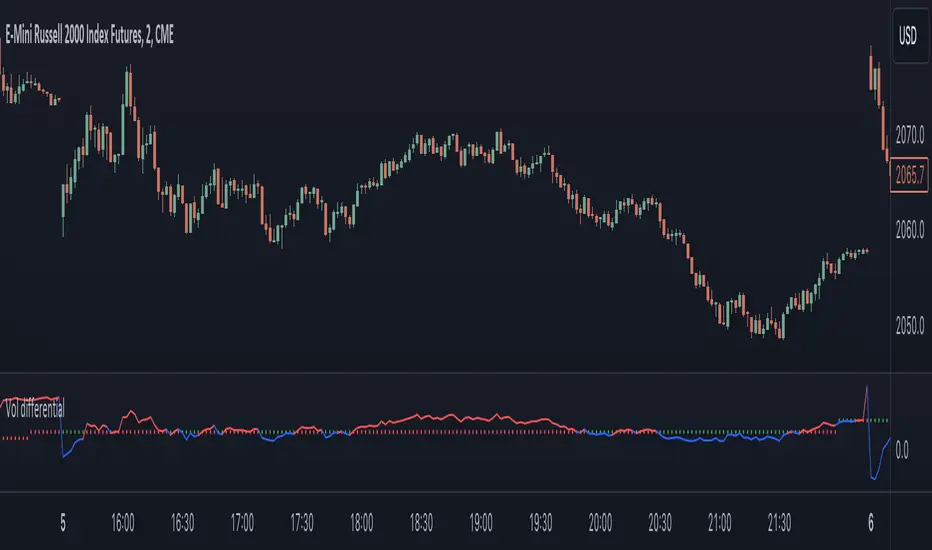
Realized volatility differentialAbout
This is a simple indicator that takes into account two types of realized volatility: Close-Close and High-Low (the latter is more useful for intraday trading).
The output of the indicator is two values / plots:
an average of High-Low volatility minus Close-Close volatility (10day period is used as a default)
the current value of the indicator
When the current value is:
lower / below the average, then it means that High-Low volatility should increase.
higher / above then obviously the opposite is true.
How to use it
It might be used as a timing tool for mean reversion strategies = when your primary strategy says a market is in mean reversion mode, you could use it as a signal for opening a position.
For example: let's say a security is in uptrend and approaching an important level (important to you).
If the current value is:
above the average, a short position can be opened, as High-Low volatility should decrease;
below the average, a trend should continue.
Intended securities
Futures contracts
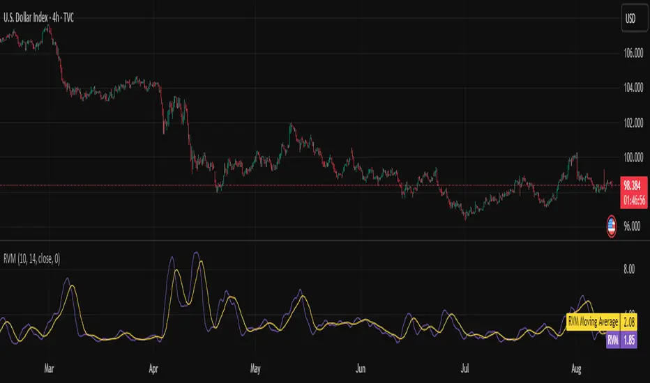
IV vs Realised Volatility (VIX/HV Comparator)VIX / HV Comparator – Implied vs Realised Volatility
This indicator compares Implied Volatility (IV) from a volatility index (VIX, India VIX, etc.) with the Realised / Historical Volatility (HV) of the current chart symbol.
It helps you see whether options are pricing volatility as rich or cheap relative to what the underlying is actually doing.
What it does
Pulls IV from any user-selected vol index symbol (e.g. CBOE:VIX for SPX, NSEINDIA:INDIAVIX for Nifty).
Calculates realised volatility from the chart’s price data using returns over a user-defined lookback.
Annualises HV so IV and HV are displayed on the same percentage scale, on any timeframe (intraday or higher).
Optionally shows an IV/HV ratio in a separate pane to highlight when options are rich or cheap relative to realised volatility.
How to read it
Main panel:
Orange line – Implied Volatility (IV) from your chosen vol index.
Aqua line – Realised / Historical Volatility (HV) of the current chart symbol.
Fill between lines:
Green shading -> IV > HV -> options are priced richer than what the underlying is currently realising.
Red shading -> HV > IV -> realised vol is higher than the options market is implying.
Sub-panel (optional):
IV / HV ratio
- Above 1 -> IV > HV (vol rich).
- Below 1 -> IV < HV (vol cheap).
- Horizontal guides (for example 1.2 / 0.8) help frame “significantly rich/cheap” zones.
A small label on the latest bar displays the current IV, HV and their difference in vol points.
Inputs (key ones)
IV Index Symbol – choose the volatility index that corresponds to your underlying (VIX, India VIX, etc.).
Realised Vol Lookback – number of bars used to compute HV (for example 20).
Trading Days per Year and Active Hours per Day – used for annualising HV so it stays consistent across timeframes.
IV Scale Factor – adjust if your IV index is quoted in decimals (0.15) instead of points (15).
Practical uses
Context for options trades – Quickly see if current IV is high or low relative to realised volatility when deciding on strategies (premium selling vs buying, spreads, hedges).
Vol regime analysis – Track shifts where HV starts to rise above IV (real stress building) or IV spikes far above HV (fear premium / insurance bid).
Cross-timeframe checks – Use on intraday charts for short-term trading context, or on daily/weekly charts for bigger picture vol regimes.
This tool is not a stand-alone signal generator. It is meant to be a volatility dashboard you combine with your usual price action, trend, and options strategy rules to understand how the options market is pricing risk vs what the underlying is actually delivering.

LS Volatility Index█ OVERVIEW
This indicator serves to measure the volatility of the price in relation to the average.
It serves four purposes:
1. Identify abnormal prices, extremely stretched in relation to an average;
2. Identify acceptable prices in the context of the main trend;
3. Identify market crashes;
4. Identify divergences.
█ CONCEPTS
The LS Volatility Index was originally described by Brazilian traders Alexandre Wolwacz (Stormer) , Fabrício Lorenz , and Fábio Figueiredo (Vlad)
Basically, this indicator can be used in two ways:
1. In a mean reversion strategy , when there is an unusual distance from it;
2. In a trend following strategy , when the price is in an acceptable region.
Perhaps the version presented here may have some slight differences, but the core is the same.
The original indicator is presented with a 21-period moving average, but here this value is customizable.
I made some fine tuning available, namely:
1. The possibility of smoothing the indicator;
2. Choose the type of moving average;
3. Customizable period;
4. Possibility to show a moving average of the indicator;
5. Color customization.
█ CALCULATION
First, the distance of the price from a given average in percentage terms is measured.
Then, the historical average volatility is obtained.
Finally the indicator is calculated through the ratio between the distance and the historical volatility.
To facilitate visualization, the result is normalized in a range from 0 to 100.
When it reaches 0, it means the price is on average.
When it hits 100, it means the price is way off average (stretched).
█ HOW TO USE IT
Here are some examples:
1. In a return-to-average strategy
2. In a trend following strategy
3. Identification of crashes and divergences
█ THANKS AND CREDITS
- Alexandre Wolwacz (Stormer), Fabrício Lorenz, Fábio Figueiredo (Vlad)
- Feature scaler (for normalization)
- HPotter (for calc of Historical Volatility)
