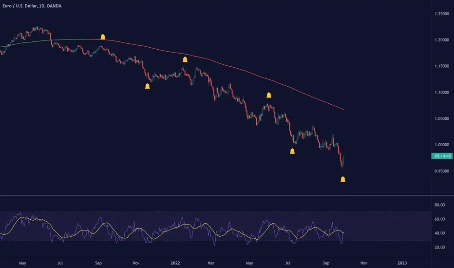
TradingView Alerts (Expo)█ Overview
The TradingView inbuilt alert feature inspires this alert tool.
TradingView Alerts (Expo) enables traders to set alerts on any indicator on TradingView, both public, protected, and invite-only scripts (if you are granted access). In this way, traders can set the alerts they want for any indicator they have access to. This feature is highly needed since many indicators on TradingView do not have the particular alert the trader looks for, this alert tool solves that problem and lets everyone create the alert they need. Many predefined conditions are included, such as "crossings," "turning up/down," "entering a channel," and much more.
█ TradingView alerts
TradingView alerts are a popular and convenient way of getting an immediate notification when the asset meets your set alert criteria. It helps traders to stay updated on the assets and timeframe they follow.
█ Alert table
Keep track of the average amount of alerts that have been triggered per day, per month, and per week. It helps traders to understand how frequently they can expect an alert to trigger.
█ Predefined alerts types
Crossing
The Crossing alert is triggered when the source input crosses (up or down) from the selected price or value.
Crossing Down / Crossing Up
The Crossing Down alert is triggered when the source input crosses down from the selected price or value.
The Crossing Up alert is triggered when the source input crosses up from the selected price or value.
Greater Than / Less Than
The Greater Than alert is triggered when the source input reaches the selected value or price.
The Less Than alert is triggered when the source input reaches the selected value or price.
Entering Channel / Exiting Channel
The Entering Channel alert is triggered when the source input enters the selected channel value.
The Exiting Channel alert is triggered when the source input exits the selected channel value.
Notice that this alert only works if you have selected "Channels."
Inside Channel / Outside Channel
The Inside Channel alert is triggered when the source input is within the selected Upper and Lower Channel boundaries.
The Outside Channel alert is triggered when the source input is outside the selected Upper and Lower Channel boundaries.
Notice that this alert only works if you have selected "Channels."
Moving Up / Moving Down
This alert is the same as "crossing up/down" within x-bars.
The Moving Up alert is triggered when the source input increases by a certain value within x-bars.
The Moving Down alert is triggered when the source input decreases by a certain value within x-bars.
Notice that you have to set the Number of Bars parameter!
The calculation starts from the last formed candlestick.
Moving Up % / Moving Down %
The Moving Up % alert is triggered when the source input increases by a certain percentage value within x-bars.
The Moving Down % alert is triggered when the source input decreases by a certain percentage value within x-bars.
Notice that you have to set the Number of Bars parameter!
The calculation starts from the last formed candlestick.
Turning Up / Turning Down
The Turning Up alert is triggered when the source input turns up.
The Turning Down alert is triggered when the source input turns down.
-----------------
Disclaimer
The information contained in my Scripts/Indicators/Ideas/Algos/Systems does not constitute financial advice or a solicitation to buy or sell any securities of any type. I will not accept liability for any loss or damage, including without limitation any loss of profit, which may arise directly or indirectly from the use of or reliance on such information.
All investments involve risk, and the past performance of a security, industry, sector, market, financial product, trading strategy, backtest, or individual's trading does not guarantee future results or returns. Investors are fully responsible for any investment decisions they make. Such decisions should be based solely on an evaluation of their financial circumstances, investment objectives, risk tolerance, and liquidity needs.
My Scripts/Indicators/Ideas/Algos/Systems are only for educational purposes!
Search in scripts for "algo"
CFB-Adaptive Velocity Histogram [Loxx]CFB-Adaptive Velocity Histogram is a velocity indicator with One-More-Moving-Average Adaptive Smoothing of input source value and Jurik's Composite-Fractal-Behavior-Adaptive Price-Trend-Period input with Dynamic Zones. All Juirk smoothing allows for both single and double Jurik smoothing passes. Velocity is adjusted to pips but there is no input value for the user. This indicator is tuned for Forex but can be used on any time series data.
What is Composite Fractal Behavior ( CFB )?
All around you mechanisms adjust themselves to their environment. From simple thermostats that react to air temperature to computer chips in modern cars that respond to changes in engine temperature, r.p.m.'s, torque, and throttle position. It was only a matter of time before fast desktop computers applied the mathematics of self-adjustment to systems that trade the financial markets.
Unlike basic systems with fixed formulas, an adaptive system adjusts its own equations. For example, start with a basic channel breakout system that uses the highest closing price of the last N bars as a threshold for detecting breakouts on the up side. An adaptive and improved version of this system would adjust N according to market conditions, such as momentum, price volatility or acceleration.
Since many systems are based directly or indirectly on cycles, another useful measure of market condition is the periodic length of a price chart's dominant cycle, (DC), that cycle with the greatest influence on price action.
The utility of this new DC measure was noted by author Murray Ruggiero in the January '96 issue of Futures Magazine. In it. Mr. Ruggiero used it to adaptive adjust the value of N in a channel breakout system. He then simulated trading 15 years of D-Mark futures in order to compare its performance to a similar system that had a fixed optimal value of N. The adaptive version produced 20% more profit!
This DC index utilized the popular MESA algorithm (a formulation by John Ehlers adapted from Burg's maximum entropy algorithm, MEM). Unfortunately, the DC approach is problematic when the market has no real dominant cycle momentum, because the mathematics will produce a value whether or not one actually exists! Therefore, we developed a proprietary indicator that does not presuppose the presence of market cycles. It's called CFB (Composite Fractal Behavior) and it works well whether or not the market is cyclic.
CFB examines price action for a particular fractal pattern, categorizes them by size, and then outputs a composite fractal size index. This index is smooth, timely and accurate
Essentially, CFB reveals the length of the market's trending action time frame. Long trending activity produces a large CFB index and short choppy action produces a small index value. Investors have found many applications for CFB which involve scaling other existing technical indicators adaptively, on a bar-to-bar basis.
What is Jurik Volty used in the Juirk Filter?
One of the lesser known qualities of Juirk smoothing is that the Jurik smoothing process is adaptive. "Jurik Volty" (a sort of market volatility ) is what makes Jurik smoothing adaptive. The Jurik Volty calculation can be used as both a standalone indicator and to smooth other indicators that you wish to make adaptive.
What is the Jurik Moving Average?
Have you noticed how moving averages add some lag (delay) to your signals? ... especially when price gaps up or down in a big move, and you are waiting for your moving average to catch up? Wait no more! JMA eliminates this problem forever and gives you the best of both worlds: low lag and smooth lines.
Ideally, you would like a filtered signal to be both smooth and lag-free. Lag causes delays in your trades, and increasing lag in your indicators typically result in lower profits. In other words, late comers get what's left on the table after the feast has already begun.
What are Dynamic Zones?
As explained in "Stocks & Commodities V15:7 (306-310): Dynamic Zones by Leo Zamansky, Ph .D., and David Stendahl"
Most indicators use a fixed zone for buy and sell signals. Here’ s a concept based on zones that are responsive to past levels of the indicator.
One approach to active investing employs the use of oscillators to exploit tradable market trends. This investing style follows a very simple form of logic: Enter the market only when an oscillator has moved far above or below traditional trading lev- els. However, these oscillator- driven systems lack the ability to evolve with the market because they use fixed buy and sell zones. Traders typically use one set of buy and sell zones for a bull market and substantially different zones for a bear market. And therein lies the problem.
Once traders begin introducing their market opinions into trading equations, by changing the zones, they negate the system’s mechanical nature. The objective is to have a system automatically define its own buy and sell zones and thereby profitably trade in any market — bull or bear. Dynamic zones offer a solution to the problem of fixed buy and sell zones for any oscillator-driven system.
An indicator’s extreme levels can be quantified using statistical methods. These extreme levels are calculated for a certain period and serve as the buy and sell zones for a trading system. The repetition of this statistical process for every value of the indicator creates values that become the dynamic zones. The zones are calculated in such a way that the probability of the indicator value rising above, or falling below, the dynamic zones is equal to a given probability input set by the trader.
To better understand dynamic zones, let's first describe them mathematically and then explain their use. The dynamic zones definition:
Find V such that:
For dynamic zone buy: P{X <= V}=P1
For dynamic zone sell: P{X >= V}=P2
where P1 and P2 are the probabilities set by the trader, X is the value of the indicator for the selected period and V represents the value of the dynamic zone.
The probability input P1 and P2 can be adjusted by the trader to encompass as much or as little data as the trader would like. The smaller the probability, the fewer data values above and below the dynamic zones. This translates into a wider range between the buy and sell zones. If a 10% probability is used for P1 and P2, only those data values that make up the top 10% and bottom 10% for an indicator are used in the construction of the zones. Of the values, 80% will fall between the two extreme levels. Because dynamic zone levels are penetrated so infrequently, when this happens, traders know that the market has truly moved into overbought or oversold territory.
Calculating the Dynamic Zones
The algorithm for the dynamic zones is a series of steps. First, decide the value of the lookback period t. Next, decide the value of the probability Pbuy for buy zone and value of the probability Psell for the sell zone.
For i=1, to the last lookback period, build the distribution f(x) of the price during the lookback period i. Then find the value Vi1 such that the probability of the price less than or equal to Vi1 during the lookback period i is equal to Pbuy. Find the value Vi2 such that the probability of the price greater or equal to Vi2 during the lookback period i is equal to Psell. The sequence of Vi1 for all periods gives the buy zone. The sequence of Vi2 for all periods gives the sell zone.
In the algorithm description, we have: Build the distribution f(x) of the price during the lookback period i. The distribution here is empirical namely, how many times a given value of x appeared during the lookback period. The problem is to find such x that the probability of a price being greater or equal to x will be equal to a probability selected by the user. Probability is the area under the distribution curve. The task is to find such value of x that the area under the distribution curve to the right of x will be equal to the probability selected by the user. That x is the dynamic zone.
Included:
Bar coloring
3 signal variations w/ alerts
Divergences w/ alerts
Loxx's Expanded Source Types
CFB-Adaptive, Williams %R w/ Dynamic Zones [Loxx]CFB-Adaptive, Williams %R w/ Dynamic Zones is a Jurik-Composite-Fractal-Behavior-Adaptive Williams % Range indicator with Dynamic Zones. These additions to the WPR calculation reduce noise and return a signal that is more viable than WPR alone.
What is Williams %R?
Williams %R , also known as the Williams Percent Range, is a type of momentum indicator that moves between 0 and -100 and measures overbought and oversold levels. The Williams %R may be used to find entry and exit points in the market. The indicator is very similar to the Stochastic oscillator and is used in the same way. It was developed by Larry Williams and it compares a stock’s closing price to the high-low range over a specific period, typically 14 days or periods.
What is Composite Fractal Behavior ( CFB )?
All around you mechanisms adjust themselves to their environment. From simple thermostats that react to air temperature to computer chips in modern cars that respond to changes in engine temperature, r.p.m.'s, torque, and throttle position. It was only a matter of time before fast desktop computers applied the mathematics of self-adjustment to systems that trade the financial markets.
Unlike basic systems with fixed formulas, an adaptive system adjusts its own equations. For example, start with a basic channel breakout system that uses the highest closing price of the last N bars as a threshold for detecting breakouts on the up side. An adaptive and improved version of this system would adjust N according to market conditions, such as momentum, price volatility or acceleration.
Since many systems are based directly or indirectly on cycles, another useful measure of market condition is the periodic length of a price chart's dominant cycle, (DC), that cycle with the greatest influence on price action.
The utility of this new DC measure was noted by author Murray Ruggiero in the January '96 issue of Futures Magazine. In it. Mr. Ruggiero used it to adaptive adjust the value of N in a channel breakout system. He then simulated trading 15 years of D-Mark futures in order to compare its performance to a similar system that had a fixed optimal value of N. The adaptive version produced 20% more profit!
This DC index utilized the popular MESA algorithm (a formulation by John Ehlers adapted from Burg's maximum entropy algorithm, MEM). Unfortunately, the DC approach is problematic when the market has no real dominant cycle momentum, because the mathematics will produce a value whether or not one actually exists! Therefore, we developed a proprietary indicator that does not presuppose the presence of market cycles. It's called CFB (Composite Fractal Behavior) and it works well whether or not the market is cyclic.
CFB examines price action for a particular fractal pattern, categorizes them by size, and then outputs a composite fractal size index. This index is smooth, timely and accurate
Essentially, CFB reveals the length of the market's trending action time frame. Long trending activity produces a large CFB index and short choppy action produces a small index value. Investors have found many applications for CFB which involve scaling other existing technical indicators adaptively, on a bar-to-bar basis.
What is Jurik Volty used in the Juirk Filter?
One of the lesser known qualities of Juirk smoothing is that the Jurik smoothing process is adaptive. "Jurik Volty" (a sort of market volatility ) is what makes Jurik smoothing adaptive. The Jurik Volty calculation can be used as both a standalone indicator and to smooth other indicators that you wish to make adaptive.
What is the Jurik Moving Average?
Have you noticed how moving averages add some lag (delay) to your signals? ... especially when price gaps up or down in a big move, and you are waiting for your moving average to catch up? Wait no more! JMA eliminates this problem forever and gives you the best of both worlds: low lag and smooth lines.
Ideally, you would like a filtered signal to be both smooth and lag-free. Lag causes delays in your trades, and increasing lag in your indicators typically result in lower profits. In other words, late comers get what's left on the table after the feast has already begun.
What are Dynamic Zones?
As explained in "Stocks & Commodities V15:7 (306-310): Dynamic Zones by Leo Zamansky, Ph .D., and David Stendahl"
Most indicators use a fixed zone for buy and sell signals. Here’ s a concept based on zones that are responsive to past levels of the indicator.
One approach to active investing employs the use of oscillators to exploit tradable market trends. This investing style follows a very simple form of logic: Enter the market only when an oscillator has moved far above or below traditional trading lev- els. However, these oscillator- driven systems lack the ability to evolve with the market because they use fixed buy and sell zones. Traders typically use one set of buy and sell zones for a bull market and substantially different zones for a bear market. And therein lies the problem.
Once traders begin introducing their market opinions into trading equations, by changing the zones, they negate the system’s mechanical nature. The objective is to have a system automatically define its own buy and sell zones and thereby profitably trade in any market — bull or bear. Dynamic zones offer a solution to the problem of fixed buy and sell zones for any oscillator-driven system.
An indicator’s extreme levels can be quantified using statistical methods. These extreme levels are calculated for a certain period and serve as the buy and sell zones for a trading system. The repetition of this statistical process for every value of the indicator creates values that become the dynamic zones. The zones are calculated in such a way that the probability of the indicator value rising above, or falling below, the dynamic zones is equal to a given probability input set by the trader.
To better understand dynamic zones, let's first describe them mathematically and then explain their use. The dynamic zones definition:
Find V such that:
For dynamic zone buy: P{X <= V}=P1
For dynamic zone sell: P{X >= V}=P2
where P1 and P2 are the probabilities set by the trader, X is the value of the indicator for the selected period and V represents the value of the dynamic zone.
The probability input P1 and P2 can be adjusted by the trader to encompass as much or as little data as the trader would like. The smaller the probability, the fewer data values above and below the dynamic zones. This translates into a wider range between the buy and sell zones. If a 10% probability is used for P1 and P2, only those data values that make up the top 10% and bottom 10% for an indicator are used in the construction of the zones. Of the values, 80% will fall between the two extreme levels. Because dynamic zone levels are penetrated so infrequently, when this happens, traders know that the market has truly moved into overbought or oversold territory.
Calculating the Dynamic Zones
The algorithm for the dynamic zones is a series of steps. First, decide the value of the lookback period t. Next, decide the value of the probability Pbuy for buy zone and value of the probability Psell for the sell zone.
For i=1, to the last lookback period, build the distribution f(x) of the price during the lookback period i. Then find the value Vi1 such that the probability of the price less than or equal to Vi1 during the lookback period i is equal to Pbuy. Find the value Vi2 such that the probability of the price greater or equal to Vi2 during the lookback period i is equal to Psell. The sequence of Vi1 for all periods gives the buy zone. The sequence of Vi2 for all periods gives the sell zone.
In the algorithm description, we have: Build the distribution f(x) of the price during the lookback period i. The distribution here is empirical namely, how many times a given value of x appeared during the lookback period. The problem is to find such x that the probability of a price being greater or equal to x will be equal to a probability selected by the user. Probability is the area under the distribution curve. The task is to find such value of x that the area under the distribution curve to the right of x will be equal to the probability selected by the user. That x is the dynamic zone.
Included:
Bar coloring
3 signal variations w/ alerts
Divergences w/ alerts
Loxx's Expanded Source Types

Intermediate Williams %R w/ Discontinued Signal Lines [Loxx]Intermediate Williams %R w/ Discontinued Signal Lines is a Williams %R indicator with advanced options:
-Williams %R smoothing, 30+ smoothing algos found here:
-Williams %R signal, 30+ smoothing algos found here:
-DSL lines with smoothing or fixed overbought/oversold boundaries, smoothing algos are EMA and FEMA
-33 Expanded Source Type inputs including Heiken-Ashi and Heiken-Ashi Better, found here:
What is Williams %R?
Williams %R, also known as the Williams Percent Range, is a type of momentum indicator that moves between 0 and -100 and measures overbought and oversold levels. The Williams %R may be used to find entry and exit points in the market. The indicator is very similar to the Stochastic oscillator and is used in the same way. It was developed by Larry Williams and it compares a stock’s closing price to the high-low range over a specific period, typically 14 days or periods.
Included:
-Toggle on/off bar coloring
-Toggle on/off signal line

OrdinaryLeastSquaresLibrary "OrdinaryLeastSquares"
One of the most common ways to estimate the coefficients for a linear regression is to use the Ordinary Least Squares (OLS) method.
This library implements OLS in pine. This implementation can be used to fit a linear regression of multiple independent variables onto one dependent variable,
as long as the assumptions behind OLS hold.
solve_xtx_inv(x, y) Solve a linear system of equations using the Ordinary Least Squares method.
This function returns both the estimated OLS solution and a matrix that essentially measures the model stability (linear dependence between the columns of 'x').
NOTE: The latter is an intermediate step when estimating the OLS solution but is useful when calculating the covariance matrix and is returned here to save computation time
so that this step doesn't have to be calculated again when things like standard errors should be calculated.
Parameters:
x : The matrix containing the independent variables. Each column is regarded by the algorithm as one independent variable. The row count of 'x' and 'y' must match.
y : The matrix containing the dependent variable. This matrix can only contain one dependent variable and can therefore only contain one column. The row count of 'x' and 'y' must match.
Returns: Returns both the estimated OLS solution and a matrix that essentially measures the model stability (xtx_inv is equal to (X'X)^-1).
solve(x, y) Solve a linear system of equations using the Ordinary Least Squares method.
Parameters:
x : The matrix containing the independent variables. Each column is regarded by the algorithm as one independent variable. The row count of 'x' and 'y' must match.
y : The matrix containing the dependent variable. This matrix can only contain one dependent variable and can therefore only contain one column. The row count of 'x' and 'y' must match.
Returns: Returns the estimated OLS solution.
standard_errors(x, y, beta_hat, xtx_inv) Calculate the standard errors.
Parameters:
x : The matrix containing the independent variables. Each column is regarded by the algorithm as one independent variable. The row count of 'x' and 'y' must match.
y : The matrix containing the dependent variable. This matrix can only contain one dependent variable and can therefore only contain one column. The row count of 'x' and 'y' must match.
beta_hat : The Ordinary Least Squares (OLS) solution provided by solve_xtx_inv() or solve().
xtx_inv : This is (X'X)^-1, which means we take the transpose of the X matrix, multiply that the X matrix and then take the inverse of the result.
This essentially measures the linear dependence between the columns of the X matrix.
Returns: The standard errors.
estimate(x, beta_hat) Estimate the next step of a linear model.
Parameters:
x : The matrix containing the independent variables. Each column is regarded by the algorithm as one independent variable. The row count of 'x' and 'y' must match.
beta_hat : The Ordinary Least Squares (OLS) solution provided by solve_xtx_inv() or solve().
Returns: Returns the new estimate of Y based on the linear model.
NormalizedOscillatorsLibrary "NormalizedOscillators"
Collection of some common Oscillators. All are zero-mean and normalized to fit in the -1..1 range. Some are modified, so that the internal smoothing function could be configurable (for example, to enable Hann Windowing, that John F. Ehlers uses frequently). Some are modified for other reasons (see comments in the code), but never without a reason. This collection is neither encyclopaedic, nor reference, however I try to find the most correct implementation. Suggestions are welcome.
rsi2(upper, lower) RSI - second step
Parameters:
upper : Upwards momentum
lower : Downwards momentum
Returns: Oscillator value
Modified by Ehlers from Wilder's implementation to have a zero mean (oscillator from -1 to +1)
Originally: 100.0 - (100.0 / (1.0 + upper / lower))
Ignoring the 100 scale factor, we get: upper / (upper + lower)
Multiplying by two and subtracting 1, we get: (2 * upper) / (upper + lower) - 1 = (upper - lower) / (upper + lower)
rms(src, len) Root mean square (RMS)
Parameters:
src : Source series
len : Lookback period
Based on by John F. Ehlers implementation
ift(src) Inverse Fisher Transform
Parameters:
src : Source series
Returns: Normalized series
Based on by John F. Ehlers implementation
The input values have been multiplied by 2 (was "2*src", now "4*src") to force expansion - not compression
The inputs may be further modified, if needed
stoch(src, len) Stochastic
Parameters:
src : Source series
len : Lookback period
Returns: Oscillator series
ssstoch(src, len) Super Smooth Stochastic (part of MESA Stochastic) by John F. Ehlers
Parameters:
src : Source series
len : Lookback period
Returns: Oscillator series
Introduced in the January 2014 issue of Stocks and Commodities
This is not an implementation of MESA Stochastic, as it is based on Highpass filter not present in the function (but you can construct it)
This implementation is scaled by 0.95, so that Super Smoother does not exceed 1/-1
I do not know, if this the right way to fix this issue, but it works for now
netKendall(src, len) Noise Elimination Technology by John F. Ehlers
Parameters:
src : Source series
len : Lookback period
Returns: Oscillator series
Introduced in the December 2020 issue of Stocks and Commodities
Uses simplified Kendall correlation algorithm
Implementation by @QuantTherapy:
rsi(src, len, smooth) RSI
Parameters:
src : Source series
len : Lookback period
smooth : Internal smoothing algorithm
Returns: Oscillator series
vrsi(src, len, smooth) Volume-scaled RSI
Parameters:
src : Source series
len : Lookback period
smooth : Internal smoothing algorithm
Returns: Oscillator series
This is my own version of RSI. It scales price movements by the proportion of RMS of volume
mrsi(src, len, smooth) Momentum RSI
Parameters:
src : Source series
len : Lookback period
smooth : Internal smoothing algorithm
Returns: Oscillator series
Inspired by RocketRSI by John F. Ehlers (Stocks and Commodities, May 2018)
rrsi(src, len, smooth) Rocket RSI
Parameters:
src : Source series
len : Lookback period
smooth : Internal smoothing algorithm
Returns: Oscillator series
Inspired by RocketRSI by John F. Ehlers (Stocks and Commodities, May 2018)
Does not include Fisher Transform of the original implementation, as the output must be normalized
Does not include momentum smoothing length configuration, so always assumes half the lookback length
mfi(src, len, smooth) Money Flow Index
Parameters:
src : Source series
len : Lookback period
smooth : Internal smoothing algorithm
Returns: Oscillator series
lrsi(src, in_gamma, len) Laguerre RSI by John F. Ehlers
Parameters:
src : Source series
in_gamma : Damping factor (default is -1 to generate from len)
len : Lookback period (alternatively, if gamma is not set)
Returns: Oscillator series
The original implementation is with gamma. As it is impossible to collect gamma in my system, where the only user input is length,
an alternative calculation is included, where gamma is set by dividing len by 30. Maybe different calculation would be better?
fe(len) Choppiness Index or Fractal Energy
Parameters:
len : Lookback period
Returns: Oscillator series
The Choppiness Index (CHOP) was created by E. W. Dreiss
This indicator is sometimes called Fractal Energy
er(src, len) Efficiency ratio
Parameters:
src : Source series
len : Lookback period
Returns: Oscillator series
Based on Kaufman Adaptive Moving Average calculation
This is the correct Efficiency ratio calculation, and most other implementations are wrong:
the number of bar differences is 1 less than the length, otherwise we are adding the change outside of the measured range!
For reference, see Stocks and Commodities June 1995
dmi(len, smooth) Directional Movement Index
Parameters:
len : Lookback period
smooth : Internal smoothing algorithm
Returns: Oscillator series
Based on the original Tradingview algorithm
Modified with inspiration from John F. Ehlers DMH (but not implementing the DMH algorithm!)
Only ADX is returned
Rescaled to fit -1 to +1
Unlike most oscillators, there is no src parameter as DMI works directly with high and low values
fdmi(len, smooth) Fast Directional Movement Index
Parameters:
len : Lookback period
smooth : Internal smoothing algorithm
Returns: Oscillator series
Same as DMI, but without secondary smoothing. Can be smoothed later. Instead, +DM and -DM smoothing can be configured
doOsc(type, src, len, smooth) Execute a particular Oscillator from the list
Parameters:
type : Oscillator type to use
src : Source series
len : Lookback period
smooth : Internal smoothing algorithm
Returns: Oscillator series
Chande Momentum Oscillator (CMO) is RSI without smoothing. No idea, why some authors use different calculations
LRSI with Fractal Energy is a combo oscillator that uses Fractal Energy to tune LRSI gamma, as seen here: www.prorealcode.com
doPostfilter(type, src, len) Execute a particular Oscillator Postfilter from the list
Parameters:
type : Oscillator type to use
src : Source series
len : Lookback period
Returns: Oscillator series

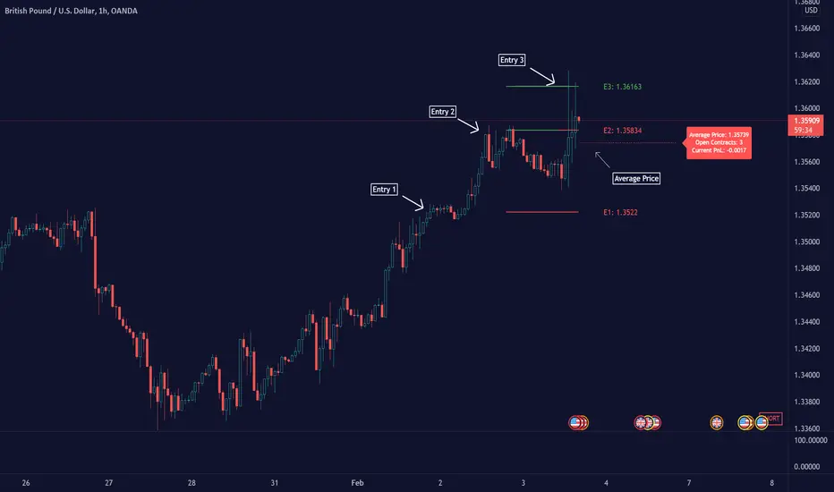
Average Down [Zeiierman]AVERAGING DOWN
Averaging down is an investment strategy that involves buying additional contracts of an asset when the price drops. This way, the investor increases the size of their position at discounted prices. The averaging down strategy is highly debated among traders and investors because it can either lead to huge losses or great returns. Nevertheless, averaging down is often used and favored by long-term investors and contrarian traders. With careful/proper risk management, averaging down can cover losses and magnify the returns when the asset rebounds. However, the main concern for a trader is that it can be hard to identify the difference between a pullback or the start of a new trend.
HOW DOES IT WORK
Averaging down is a method to lower the average price at which the investor buys an asset. A lower average price can help investors come back to break even quicker and, if the price continues to rise, get an even bigger upside and thus increase the total profit from the trade. For example, We buy 100 shares at $60 per share, a total investment of $6000, and then the asset drops to $40 per share; in order to come back to break even, the price has to go up 50%. (($60/$40) - 1)*100 = 50%.
The power of Averaging down comes into play if the investor buys additional shares at a lower price, like another 100 shares at $40 per share; the total investment is ($6000+$4000 = $10000). The average price for the investment is now $50. (($60 x 100) + ($40 x 100))/200; in order to get back to break even, the price has to rise 25% ($50/$40)-1)*100 = 25%, and if the price continues up to $60 per share, the investor can secure a profit at 16%. So by averaging down, investors and traders can cover the losses easier and potentially have more profit to secure at the end.
THE AVERAGE DOWN TRADINGVIEW TOOL
This script/indicator/trading tool helps traders and investors to get the average price of their position. The tool works for Long and Short and displays the entry price, average price, and the PnL in points.
HOW TO USE
Use the tool to calculate the average price of your long or short position in any market and timeframe.
Get the current PnL for the investment and keep track of your entry prices.
APPLY TO CHART
When you apply the tool on the chart, you have to select five entry points, and within the setting panel, you can choose how many of these five entry points are active and how many contracts each entry has. Then, the tool will display your average price based on the entries and the number of contracts used at each price level.
LONG
Set your entries and the number of contracts at each price level. The indicator will then display all your long entries and at what price you will break even. The entry line changes color based on if the entry is in profit or loss.
SHORT
Set your entries and the number of contracts at each price level. The indicator will then display all your short entries and at what price you will break even. The entry line changes color based on if the entry is in profit or loss.
-----------------
Disclaimer
Copyright by Zeiierman.
The information contained in my Scripts/Indicators/Ideas/Algos/Systems does not constitute financial advice or a solicitation to buy or sell any securities of any type. I will not accept liability for any loss or damage, including without limitation any loss of profit, which may arise directly or indirectly from the use of or reliance on such information.
All investments involve risk, and the past performance of a security, industry, sector, market, financial product, trading strategy, backtest, or individual’s trading does not guarantee future results or returns. Investors are fully responsible for any investment decisions they make. Such decisions should be based solely on an evaluation of their financial circumstances, investment objectives, risk tolerance, and liquidity needs.
My Scripts/Indicators/Ideas/Algos/Systems are only for educational purposes!
Example: Monte Carlo SimulationExperimental:
Example execution of Monte Carlo Simulation applied to the markets(this is my interpretation of the algo so inconsistencys may appear).
note:
the algorithm is very demanding so performance is limited.
Weis pip zigzag jayyWhat you see here is the Weis pip zigzag wave plotted directly on the price chart. This script is the companion to the Weis pip wave ( ) which is plotted in the lower panel of the displayed chart and can be used as an alternate way of plotting the same results. The Weis pip zigzag wave shows how far in terms of price a Weis wave has traveled through the duration of a Weis wave. The Weis pip zigzag wave is used in combination with the Weis cumulative volume wave. The two waves must be set to the same "wave size".
To use this script you must set the wave size. Using the traditional Weis method simply enter the desired wave size in the box "Select Weis Wave Size" In this example, it is set to 5. Each wave for each security and each timeframe requires its own wave size. Although not the traditional method a more automatic way to set wave size would be to use ATR. This is not the true Weis method but it does give you similar waves and, importantly, without the hassle described above. Once the Weis wave size is set then the pip wave will be shown.
I have put a pip zigzag of a 5 point Weis wave on the bar chart - that is a different script. I have added it to allow your eye to see what a Weis wave looks like. You will notice that the wave is not in straight lines connecting wave tops to bottoms this is a function of the limitations of Pinescript version 1. This script would need to be in version 4 to allow straight lines. There are too many calculations within this script to allow conversion to Pinescript version 4 or even Version 3. I am in the process of rewriting this script to reduce the number of calculations and streamline the algorithm.
The numbers plotted on the chart are calculated to be relative numbers. The script is limited to showing only three numbers vertically. Only the highest three values of a number are shown. For example, if the highest recent pip value is 12,345 only the first 3 numerals would be displayed ie 123. But suppose there is a recent value of 691. It would not be helpful to display 691 if the other wave size is shown as 123. To give the appropriate relative value the script will show a value of 7 instead of 691. This informs you of the relative magnitude of the values. This is done automatically within the script. There is likely no need to manually override the automatically calculated value. I will create a video that demonstrates the manual override method.
What is a Weis wave? David Weis has been recognized as a Wyckoff method analyst he has written two books one of which, Trades About to Happen, describes the evolution of the now popular Weis wave. The method employed by Weis is to identify waves of price action and to compare the strength of the waves on characteristics of wave strength. Chief among the characteristics of strength is the cumulative volume of the wave. There are other markers that Weis uses as well for example how the actual price difference between the start of the Weis wave from start to finish. Weis also uses time, particularly when using a Renko chart. Weis specifically uses candle or bar closes to define all wave action ie a line chart.
David Weis did a futures io video which is a popular source of information about his method.
This is the identical script with the identical settings but without the offending links. If you want to see the pip Weis method in practice then search Weis pip wave. If you want to see Weis chart in pdf then message me and I will give a link or the Weis pdf. Why would you want to see the Weis chart for May 27, 2020? Merely to confirm the veracity of my algorithm. You could compare my Weis chart here () from the same period to the David Weis chart from May 27. Both waves are for the ES!1 4 hour chart and both for a wave size of 5.
Price Action and 3 EMAs Momentum plus Sessions FilterThis indicator plots on the chart the parameters and signals of the Price Action and 3 EMAs Momentum plus Sessions Filter Algorithmic Strategy. The strategy trades based on time-series (absolute) and relative momentum of price close, highs, lows and 3 EMAs.
I am still learning PS and therefore I have only been able to write the indicator up to the Signal generation. I plan to expand the indicator to Entry Signals as well as the full Strategy.
The strategy works best on EURUSD in the 15 minutes TF during London and New York sessions with 1 to 1 TP and SL of 30 pips with lots resulting in 3% risk of the account per trade. I have already written the full strategy in another language and platform and back tested it for ten years and it was profitable for 7 of the 10 years with average profit of 15% p.a which can be easily increased by increasing risk per trade. I have been trading it live in that platform for over two years and it is profitable.
Contributions from experienced PS coders in completing the Indicator as well as writing the Strategy and back testing it on Trading View will be appreciated.
STRATEGY AND INDICATOR PARAMETERS
Three periods of 12, 48 and 96 in the 15 min TF which are equivalent to 3, 12 and 24 hours i.e (15 min * period / 60 min) are the foundational inputs for all the parameters of the PA & 3 EMAs Momentum + SF Algo Strategy and its Indicator.
3 EMAs momentum parameters and conditions
• FastEMA = ema of 12 periods
• MedEMA = ema of 48 periods
• SlowEMA = ema of 96 periods
• All the EMAs analyse price close for up to 96 (15 min periods) equivalent to 24 hours
• There’s Upward EMA momentum if price close > FastEMA and FastEMA > MedEMA and MedEMA > SlowEMA
• There’s Downward EMA momentum if price close < FastEMA and FastEMA < MedEMA and MedEMA < SlowEMA
PA momentum parameters and conditions
• HH = Highest High of 48 periods from 1st closed bar before current bar
• LL = Lowest Low of 48 periods from 1st closed bar from current bar
• Previous HH = Highest High of 84 periods from 12th closed bar before current bar
• Previous LL = Lowest Low of 84 periods from 12th closed bar before current bar
• All the HH & LL and prevHH & prevLL are within the 96 periods from the 1st closed bar before current bar and therefore indicative of momentum during the past 24 hours
• There’s Upward PA momentum if price close > HH and HH > prevHH and LL > prevLL
• There’s Downward PA momentum if price close < LL and LL < prevLL and HH < prevHH
Signal conditions and Status (BuySignal, SellSignal or Neutral)
• The strategy generates Buy or Sell Signals if both 3 EMAs and PA momentum conditions are met for each direction and these occur during the London and New York sessions
• BuySignal if price close > FastEMA and FastEMA > MedEMA and MedEMA > SlowEMA and price close > HH and HH > prevHH and LL > prevLL and timeinrange (LDN&NY) else Neutral
• SellSignal if price close < FastEMA and FastEMA < MedEMA and MedEMA < SlowEMA and price close < LL and LL < prevLL and HH < prevHH and timeinrange (LDN&NY) else Neutral
Entry conditions and Status (EnterBuy, EnterSell or Neutral)(NOT CODED YET)
• ENTRY IS NOT AT THE SIGNAL BAR but at the current bar tick price retracement to FastEMA after the signal
• EnterBuy if current bar tick price <= FastEMA and current bar tick price > prevHH at the time of the Buy Signal
• EnterSell if current bar tick price >= FastEMA and current bar tick price > prevLL at the time of the Sell Signal

NAND PerceptronExperimental NAND Perceptron based upon Python template that aims to predict NAND Gate Outputs. A Perceptron is one of the foundational building blocks of nearly all advanced Neural Network layers and models for Algo trading and Machine Learning.
The goal behind this script was threefold:
To prove and demonstrate that an ACTUAL working neural net can be implemented in Pine, even if incomplete.
To pave the way for other traders and coders to iterate on this script and push the boundaries of Tradingview strategies and indicators.
To see if a self-contained neural network component for parameter optimization within Pinescript was hypothetically possible.
NOTE: This is a highly experimental proof of concept - this is NOT a ready-made template to include or integrate into existing strategies and indicators, yet (emphasis YET - neural networks have a lot of potential utility and potential when utilized and implemented properly).
Hardcoded NAND Gate outputs with Bias column (X0):
// NAND Gate + X0 Bias and Y-true
// X0 // X1 // X2 // Y
// 1 // 0 // 0 // 1
// 1 // 0 // 1 // 1
// 1 // 1 // 0 // 1
// 1 // 1 // 1 // 0
Column X0 is bias feature/input
Column X1 and X2 are the NAND Gate
Column Y is the y-true values for the NAND gate
yhat is the prediction at that timestep
F0,F1,F2,F3 are the Dot products of the Weights (W0,W1,W2) and the input features (X0,X1,X2)
Learning rate and activation function threshold are enabled by default as input parameters
Uncomment sections for more training iterations/epochs:
Loop optimizations would be amazing to have for a selectable length for training iterations/epochs but I'm not sure if it's possible in Pine with how this script is structured.
Error metrics and loss have not been implemented due to difficulty with script length and iterations vs epochs - I haven't been able to configure the input parameters to successfully predict the right values for all four y-true values for the NAND gate (only been able to get 3/4; If you're able to get all four predictions to be correct, let me know, please).
// //---- REFERENCE for final output
// A3 := 1, y0 true
// B3 := 1, y1 true
// C3 := 1, y2 true
// D3 := 0, y3 true
PLEASE READ: Source article/template and main code reference:
towardsdatascience.com
towardsdatascience.com
towardsdatascience.com
Baseline-C [ID: AC-P]The "AC-P" version of jiehonglim's NNFX Baseline script is my personal customized version of the NNFX Baseline concept as part of the NNFX Algorithm stack/structure for 1D Trend Trading for Forex. Everget's JMA implementation is used for the baseline smoothing method, with optional ATR bands at 1.0x and 1.5x from the baseline.
NNFX = No Nonsense Forex
Baseline = Component of the NNFX Algorithm that consists of a single moving average
Baseline ---> Meant to be used in conjunction with ATR/C1/C2/Vol Indicator/Exit Indicator as per NNFX Algorithm setup/structure. C1 is 1st Confirmation Indicator, C2 is 2nd Confirmation Indicator.
JMA (Jurik Moving Average) is used for the baseline and slow baseline.
A slow baseline option is included, but disabled by default.
The faint orange/purple lines are 1.0x/1.5x ATR from the Baseline, and are what I use as potential TP/SL targets or to evaluate when to stay out of a trade (chop/missed entry/exit/other/ATR breach), depending on the trade setup (in conjunction with C1/C2/Vol Indicator/Exit Indicator)
This script is heavily based upon jiehonglim's NNFX Baseline script for signaling, barcoloring, and ATR.
SSL Channel option included but disabled by default (Erwinbeckers SSL component)
POC (Point of Control) from Volume Profile is included/enabled by default for both the current timeframe and 12HR timeframe
03.freeman's InfoPanel Divergence Indicator was used a reference to replace the current/previous ATR information infopanel/info draw from jiehonglim's script. I'm not sure whether I like the previous way ATR info was displayed vs how I have it currently, but it's something that is completely optional:
Specifically: I am tuning this baseline/indicator for 1D trading as part of the NNFX system, for Forex.
DO NOT USE THIS INDICATOR WITHOUT PROPER TUNING/ADJUSTMENT for your timeframe and asset class.
Note about lack of alerts:
Alerts for baseline crosses (and other crosses) have been purposefully omitted for this version upon initial publication. While getting alerts for baseline crosses under certain conditions/filtered conditions that eliminate low-importance signals and crossover whipsaw would be great, it's something I'm still looking into.
SPECIFICALLY: There are entry, exit, take profit, and continuation signal components in relation to the Baseline to the rest of the NNFX Algorithm stack (ATR/C1/C2/Vol Indicator/Exit Indicator), including but limited to the "1 candle rule" and the "7 candle rule" as per NNFX.
Implementing alerts that are significant that also factor in these rules while reducing alert spam/false signals would be ideal, but it's also the HTF/Daily chart - visually, entry/exit/continuation signal alignment is easy to spot when trading 1D - alerts may be redundant/a pursuit in diminishing returns (for now).
//-------------------------------------------------------------------
// Acknowledgements/Reference:
// jiehonglim, NNFX Baseline Script - Moving Averages
//
// Fractured, Many Moving Averages
//
// everget, Jurik Moving Average/JMA
//
// 03.freeman, InfoPanel Divergence Indicator
//
// Ggqmna Volume stops
//
// Libertus RSI Divs
//
// ChrisMoody, CM_Price-Action-Bars-Price Patterns That Work
//
// Erwinbeckers SSL Channel
//

WickPressureLibWickPressureLib: The Regime Dynamics Engine
DESCRIPTION:
WickPressureLib/b] is not a standard candlestick pattern library. It is an advanced analytical engine designed to deconstruct the internal dynamics of price action. It provides a definitive toolkit for analyzing candle microstructure and quantifying order flow pressure through statistical modeling.
█ CHAPTER 1: THE PHILOSOPHY — BEYOND PATTERNS, INTO DYNAMICS
A candlestick wick represents a specific market event: a rejection of price. Traditional analysis often labels these simply as "bullish" or "bearish." This library aims to go deeper by treating each candle as a dataset of opposing forces.
The WickPressureLib translates static price action into dynamic metrics. It deconstructs the candle into core components and subjects them to multi-layered analysis. It calculates Kinetic Force , estimates institutional Delta , tracks the Siege Decay of key levels, and uses Thompson Sampling (a Bayesian probability algorithm) to assess the statistical weight of each formation.
This library does not just identify patterns; it quantifies the forces that create them. It is designed for developers who need quantitative, data-driven metrics rather than subjective interpretation.
█ CHAPTER 2: THE ANALYTICAL PIPELINE — SIX LAYERS OF LOGIC
The engine's capabilities come from a six-stage processing pipeline. Each layer builds upon the last to create a comprehensive data object.
LAYER 1 — DELTA ESTIMATION: Uses a proprietary model to approximate order flow (Delta) within a single candle based on the relationship between wicks, body, and total range.
LAYER 2 — SIEGE ANALYSIS: A concept for measuring structural integrity. Every time a price level is tested by a wick, its "Siege Decay" score is updated. Repeated tests without a breakout result in a decayed score, indicating weakening support/resistance.
LAYER 3 — MAGNETISM ENGINE: Calculates the probability of a wick being "filled" (mean reversion) based on trend strength and volume profile. Distinguishes between rejection wicks and exhaustion wicks.
LAYER 4 — REGIME DETECTION: Context-aware analysis using statistical tools— Shannon Entropy (disorder), DFA (trend vs. mean-reversion), and Hurst Exponent (persistence)—to classify the market state (e.g., "Bull Trend," "Bear Range," "Choppy").
LAYER 5 — ADAPTIVE LEARNING (THOMPSON SAMPLING): Uses a Bayesian Multi-Armed Bandit algorithm to track performance. It maintains a set of "Agents," each tracking a different wick pattern type. Based on historical outcomes, the system updates the probability score for each pattern in real-time.
LAYER 6 — CONTEXTUAL ROUTING: The final layer of logic. The engine analyzes the wick, determines its pattern type, and routes it to the appropriate Agent for probability assessment, weighted by the current market regime.
█ CHAPTER 3: CORE FUNCTIONS
analyze_wick() — The Master Analyzer
The primary function. Accepts a bar index and returns a WickAnalysis object containing over 15 distinct metrics:
• Anomaly Score: Z-Score indicating how statistically rare the wick's size is.
• Kinetic Force: Metric combining range and relative volume to quantify impact.
• Estimated Delta: Approximation of net buying/selling pressure.
• Siege Decay: Structural integrity of the tested level.
• Magnet Score: Probability of the wick being filled.
• Win Probability: Adaptive success rate based on the Thompson Sampling engine.
scan_clusters() — Liquidity Zone Detection
Scans recent price history to identify "Pressure Clusters"—zones where multiple high-pressure wicks have overlapped. Useful for finding high-probability supply and demand zones.
detect_regime() — Context Engine
Uses statistical methods to determine the market's current personality (Trending, Ranging, or Volatile). This output allows the analysis to adapt dynamically to changing conditions.
█ CHAPTER 4: DEVELOPER INTEGRATION GUIDE
This library is a low-level engine for building sophisticated indicators.
1. Import the Library:
import DskyzInvestments/DafeWickLib/1 as wpk
2. Initialize the Agents:
var agents = wpk.create_learning_agents()
3. Analyze the Market:
regime = wpk.detect_regime(100)
wick_data = wpk.analyze_wick(0, regime, agents)
prob = wpk.get_probability(wick_data, regime)
4. Update Learning (Feedback Loop):
agent_id = wpk.get_agent_by_pattern(wick_data)
agents := wpk.update_learning_agent(agents, agent_id, 1.0) // +1 win, -1 loss
█ CHAPTER 5: THE DEVELOPER'S FRAMEWORK — INTEGRATION GUIDE
This library serves as a professional integration framework. This guide provides instructions and templates required to connect the DAFE components into a unified custom Pine Script indicator.
PART I: THE INPUTS TEMPLATE (CONTROL PANEL)
To provide users full control over the system, include the input templates from all connected libraries. This section details the bridge-specific controls.
// ╔═════════════════════════════════════════════════════════╗
// ║ BRIDGE INPUTS TEMPLATE (COPY INTO YOUR SCRIPT) ║
// ╚═════════════════════════════════════════════════════════╝
// INPUT GROUPS
string G_BRIDGE_MAIN = "════════════ 🌉 BRIDGE CONFIG ════════════"
string G_BRIDGE_EXT = "════════════ 🌐 EXTERNAL DATA ════════════"
// BRIDGE MAIN CONFIG
float i_bridge_min_conf = input.float(0.55, "Min Confidence to Trade",
minval=0.4, maxval=0.8, step=0.01, group=G_BRIDGE_MAIN,
tooltip="Minimum blended confidence required for a trade signal.")
int i_bridge_warmup = input.int(100, "System Warmup Bars",
minval=50, maxval=500, group=G_BRIDGE_MAIN,
tooltip="Bars required for data gathering before signals begin.")
// EXTERNAL DATA SOCKETS
bool i_ext_enable = input.bool(true, "🌐 Enable External Data Sockets",
group=G_BRIDGE_EXT,
tooltip="Enables analysis of external market data (e.g., VIX, DXY).")
// Example for one external socket
string i_ext1_name = input.string("VIX", "Socket 1: Name", group=G_BRIDGE_EXT, inline="ext1")
string i_ext1_sym = input.symbol("TVC:VIX", "Symbol", group=G_BRIDGE_EXT, inline="ext1")
string i_ext1_type = input.string("volatility", "Data Type",
options= ,
group=G_BRIDGE_EXT, inline="ext1")
float i_ext1_weight = input.float(1.0, "Weight", minval=0.1, maxval=2.0, step=0.1, group=G_BRIDGE_EXT, inline="ext1")
PART II: IMPLEMENTATION LOGIC (THE CORE LOOP)
This boilerplate code demonstrates the complete, unified pipeline structure.
// ╔════════════════════════════════════════════════════════╗
// ║ USAGE EXAMPLE (ADAPT TO YOUR SCRIPT) ║
// ╚════════════════════════════════════════════════════════╝
// 1. INITIALIZE ENGINES (First bar only)
var rl.RLAgent agent = rl.init(...)
var spa.SPAEngine spa_engine = spa.init(...)
var bridge.BridgeState bridge_state = bridge.init_bridge(i_spa_num_arms, i_rl_num_actions, i_bridge_min_conf, i_bridge_warmup)
// 2. CONNECT SOCKETS (First bar only)
if barstate.isfirst
// Connect internal sockets
agent := rl.connect_socket(agent, "rsi", ...)
// Register external sockets
if i_ext_enable
ext_socket_1 = bridge.create_ext_socket(i_ext1_name, i_ext1_sym, i_ext1_type, i_ext1_weight)
bridge_state := bridge.register_ext_socket(bridge_state, ext_socket_1)
// 3. MAIN LOOP (Every bar)
// --- A. UPDATE EXTERNAL DATA ---
if i_ext_enable
= request.security(i_ext1_sym, timeframe.period, )
bridge_state := bridge.update_ext_by_name(bridge_state, i_ext1_name, ext1_c, ext1_h, ext1_l)
bridge_state := bridge.aggregate_ext_sockets(bridge_state)
// --- B. RL/ML PROPOSES ---
rl.RLState ml_state = rl.build_state(agent)
= rl.select_action(agent, ml_state)
agent := updated_agent
// --- C. BRIDGE TRANSLATES ---
array arm_signals = bridge.generate_arm_signals(ml_action.action, ml_action.confidence, i_spa_num_arms, i_rl_num_actions, 0)
// --- D. SPA DISPOSES ---
spa_engine := spa.feed_signals(spa_engine, arm_signals, close)
= spa.select(spa_engine)
spa_engine := updated_spa
string arm_name = spa.get_name(spa_engine, selected_arm)
// --- E. RECONCILE REGIME & COMPUTE RISK ---
bridge_state := bridge.reconcile_regime(bridge_state, ml_regime_id, ml_regime_name, ml_conf, spa_regime_id, spa_conf, ...)
float risk = bridge.compute_risk(bridge_state, ml_action.confidence, spa_conf, ...)
// --- F. MAKE FINAL DECISION ---
bridge_state := bridge.make_decision(bridge_state, ml_action.action, ml_action.confidence, selected_arm, arm_name, final_spa_signal, spa_conf, risk, 0.25)
bridge.UnifiedDecision final_decision = bridge_state.decision
// --- G. EXECUTE ---
if final_decision.should_trade
// Plot signals, manage positions based on final_decision.direction
// --- H. LEARN (FEEDBACK LOOP) ---
if (trade_is_closed)
bridge_state := bridge.compute_reward(bridge_state, selected_arm, ...)
agent := rl.learn(agent, ..., bridge_state.reward.shaped_reward, ...)
// --- I. PERFORMANCE & DIAGNOSTICS ---
bridge_state := bridge.update_performance(bridge_state, actual_market_direction)
if barstate.islast
label.new(bar_index, high, bridge.bridge_diagnostics(bridge_state), textalign=text.align_left)
█ DEVELOPMENT PHILOSOPHY
DafeMLSPABridge represents a hierarchical design philosophy. We believe robust systems rely not on a single algorithm, but on the intelligent integration of specialized subsystems. A complete trading logic requires tactical precision (ML), strategic selection (SPA), and environmental awareness (External Sockets). This library provides the infrastructure for these components to communicate and coordinate.
█ DISCLAIMER & IMPORTANT NOTES
• LIBRARY FOR DEVELOPERS: This script is an integration tool and produces no output on its own. It requires implementation of DafeRLMLLib and DafeSPALib.
• COMPUTATION: Full bridged systems are computationally intensive.
• RISK: All automated decisions are based on statistical probabilities from historical data. They do not predict future market movements with certainty.
"The whole is greater than the sum of its parts." — Aristotle
Create with DAFE.

Acrobatic Loto Predictor [Taolue Remix]
市場のカオスを、幸運の数字へ。
このインジケーターは、現在のチャートの「価格変動」「時間」「ボラティリティ」を複雑な計算式(カオス力学)に通すことで、 Loto 6 (6/43) および Loto 7 (7/37) の予想数字を算出する実験的なツールです。
単なるランダム生成(乱数)ではありません。RSIやボリンジャーバンドといったテクニカル指標の数値を「乱数の種(シード)」として使用しているため、 「相場の息遣い」がそのまま数字として出力されます。
【主な機能】
1. モード: 設定画面から「Loto 6」と「Loto 7」を切り替え可能です。
2. カオス&テクニカル・ロジック:
- カオス力学: ローレンツ・アトラクタに着想を得た非線形計算。
- テクニカル: RSI(相対力指数)とボリンジャーバンドの位置関係を係数化。
- 概念定数: 黄金比(φ)や特定の数学的定数を隠し味に配合。
3. ストップ(固定)機能: チャートが動くたびに数字は変動しますが、「ここだ!」と思った瞬間にチェックボックスで数字を 完全固定(ロック) できます。
4. リロール(再抽選)機能: 固定した数字が気に入らない場合、リロール値を変更することで、その瞬間のパラレルワールド(別の計算結果)を呼び出せます。
5. ディスコモード: 数字が変動している間は背景色がリズミカルに変化し、固定すると色が落ち着く視覚効果付き。
【使い方】
1. チャートに追加します(ビットコインや為替など、動きのある銘柄推奨)。
2. 設定画面で Loto 6 か Loto 7 を選びます。
3. チャートを眺め、相場の「波」を感じます。
4. 直感的に良いタイミングで設定画面の 「ストップ(数値を固定)」 にチェックを入れます。
5. 表示された数字をメモします。(気に入らなければ「結果のリロール」数値を変更してください)
※免責事項:
このツールはエンターテインメント目的で作成されています。当選を保証するものではありません。宝くじの購入は自己責任で楽しみましょう。
---
Transform Market Chaos into Lucky Numbers.
This indicator is an experimental tool that generates predictions for Loto 6 and Loto 7 by feeding current chart data—price action, time, and volatility—into complex chaotic algorithms.
This is not a simple random number generator. It uses technical indicators like RSI and Bollinger Bands as "seeds" for generation. Essentially, the heartbeat of the market decides your numbers.
1. Mode: Switch between "Loto 6" (pick 6 from 43) and "Loto 7" (pick 7 from 37) in the settings.
2. Chaos & Technical Logic:
- Chaos Dynamics: Non-linear calculations inspired by the Lorentz Attractor.
- Technical Analysis: Weighing factors based on RSI and Bollinger Band positioning.
- Conceptual Constants: Incorporates the Golden Ratio (φ) and other mathematical constants.
3. Freeze/Lock Function: Numbers fluctuate with every tick. Use the "Stop" checkbox to lock the numbers at the exact moment you feel the market energy align.
4. Reroll System: If you lock the numbers but don't like the result, change the "Reroll" value to access a parallel timeline (alternate calculation result) for the same candle.
5. Disco Visuals: Background colors dance rhythmically while spinning and settle down when locked.
1. Add to chart (highly volatile assets like BTC or FX recommended).
2. Select Loto 6 or Loto 7 in the settings.
3. Watch the chart and feel the "wave" of the market.
4. Check the "Stop (Lock Numbers)" box in settings when your intuition strikes.
5. Note down the numbers. (Use the "Reroll" input if you want to reshape your destiny).
This tool is for entertainment purposes only. It does not guarantee any lottery winnings. Please play responsibly.

Acrobatic Loto Predictor [Taolue Remix]市場のカオスを、幸運の数字へ。
このインジケーターは、現在のチャートの「価格変動」「時間」「ボラティリティ」を複雑な計算式(カオス力学)に通すことで、 Loto 6 (6/43) および Loto 7 (7/37) の予想数字を算出する実験的なツールです。
単なるランダム生成(乱数)ではありません。RSIやボリンジャーバンドといったテクニカル指標の数値を「乱数の種(シード)」として使用しているため、 「相場の息遣い」がそのまま数字として出力されます。
【主な機能】
1. モード: 設定画面から「Loto 6」と「Loto 7」を切り替え可能です。
2. カオス&テクニカル・ロジック:
- カオス力学: ローレンツ・アトラクタに着想を得た非線形計算。
- テクニカル: RSI(相対力指数)とボリンジャーバンドの位置関係を係数化。
- 概念定数: 黄金比(φ)や特定の数学的定数を隠し味に配合。
3. ストップ(固定)機能: チャートが動くたびに数字は変動しますが、「ここだ!」と思った瞬間にチェックボックスで数字を 完全固定(ロック) できます。
4. リロール(再抽選)機能: 固定した数字が気に入らない場合、リロール値を変更することで、その瞬間のパラレルワールド(別の計算結果)を呼び出せます。
5. ディスコモード: 数字が変動している間は背景色がリズミカルに変化し、固定すると色が落ち着く視覚効果付き。
【使い方】
1. チャートに追加します(ビットコインや為替など、動きのある銘柄推奨)。
2. 設定画面で Loto 6 か Loto 7 を選びます。
3. チャートを眺め、相場の「波」を感じます。
4. 直感的に良いタイミングで設定画面の 「ストップ(数値を固定)」 にチェックを入れます。
5. 表示された数字をメモします。(気に入らなければ「結果のリロール」数値を変更してください)
※免責事項:
このツールはエンターテインメント目的で作成されています。当選を保証するものではありません。宝くじの購入は自己責任で楽しみましょう。
---
Transform Market Chaos into Lucky Numbers.
This indicator is an experimental tool that generates predictions for Loto 6 and Loto 7 by feeding current chart data—price action, time, and volatility—into complex chaotic algorithms.
This is not a simple random number generator. It uses technical indicators like RSI and Bollinger Bands as "seeds" for generation. Essentially, the heartbeat of the market decides your numbers.
1. Mode: Switch between "Loto 6" (pick 6 from 43) and "Loto 7" (pick 7 from 37) in the settings.
2. Chaos & Technical Logic:
- Chaos Dynamics: Non-linear calculations inspired by the Lorentz Attractor.
- Technical Analysis: Weighing factors based on RSI and Bollinger Band positioning.
- Conceptual Constants: Incorporates the Golden Ratio (φ) and other mathematical constants.
3. Freeze/Lock Function: Numbers fluctuate with every tick. Use the "Stop" checkbox to lock the numbers at the exact moment you feel the market energy align.
4. Reroll System: If you lock the numbers but don't like the result, change the "Reroll" value to access a parallel timeline (alternate calculation result) for the same candle.
5. Disco Visuals: Background colors dance rhythmically while spinning and settle down when locked.
1. Add to chart (highly volatile assets like BTC or FX recommended).
2. Select Loto 6 or Loto 7 in the settings.
3. Watch the chart and feel the "wave" of the market.
4. Check the "Stop (Lock Numbers)" box in settings when your intuition strikes.
5. Note down the numbers. (Use the "Reroll" input if you want to reshape your destiny).
This tool is for entertainment purposes only. It does not guarantee any lottery winnings. Please play responsibly.

Mine Shaft + Drift + Ore Pocket Detector (Gap+Touch)Mine Shaft + Drift + Ore Pocket Detector (Gap+Touch) — Full Description (v1.6.1, Pine v6)
*Experimental - *Test Phase*
1) What this indicator is intended to do
This indicator attempts to algorithmically discover “mine shaft” price structure on a chart by:
Collecting structural anchor points (gaps and optionally pivots),
Generating candidate trend “rails” (centerline + parallel upper/lower borders) from pairs of anchors,
Fitting an optimal channel width around each candidate centerline,
Scoring candidates based on how well price action conforms to the channel (touches + containment),
Selecting and rendering:
the main shaft channel (primary),
additional drifts (secondary shafts per direction),
And then detecting Ore Pockets: time locations where multiple selected lines intersect (time confluence / intersection clustering).
The conceptual model is:
A shaft = a best-fit channel that price respects over time (the “main tunnel”).
Drifts = alternate channels close in quality to the main shaft (secondary tunnels).
Ore pockets = future/past time coordinates where multiple channels’ centerlines intersect densely (confluence in time, not necessarily in price).
2) What it is doing right now (current behavior)
In its current form, the script does a bounded, performance-limited scan:
It stores a limited number of anchor points in arrays.
It only considers a bounded number of recent anchors per direction.
It constructs candidate lines from anchor pairs and evaluates channel fitness using sampled bars.
On the last bar, it selects top candidates per direction and draws:
a “main” channel per mode (single best overall, or separate up/down),
plus optional drift channels,
plus ore pocket markers.
It is producing meaningful channels and drifts, but it is currently more likely to lock onto a strong “local” shaft than the one macro shaft spanning the entire market structure.
3) Core mechanics (how the script finds shafts)
3.1 Anchor generation (what points it uses)
Anchors are the “support points” used to build candidate shaft centerlines.
Two anchor families are supported:
A) Gap anchors (from your selected gap mode)
These attempt to capture “displacement events” and their boundaries/mids.
B) Pivot anchors (optional structural anchors)
These use pivots to inject macro structure points that are not strictly gap-based.
All anchors are stored as:
anchorX: bar_index of anchor
anchorY: price of anchor
anchorD: direction flag (+1 for up, -1 for down)
Anchors are capped by maxAnchors with FIFO trimming.
3.2 Candidate generation (how it produces centerlines)
For each direction (+1 and -1):
Collect “recent” anchors of that direction within lookbackBars (bounded to maxDirAnchors).
For each pair of anchors (x1,y1) and (x2,y2) that satisfy:
spacing within ,
slope sign consistent with direction,
Construct the line equation:
slope m and intercept b
Fit a channel width w around that line (via width mode).
Score it (touches + inside count minus width penalty).
Keep the top K rails (K = driftCount+1 typically).
3.3 Scoring model (what “best” means right now)
For a candidate centerline:
At sampled bars (stride sampling), compute:
channel top = y(x) + w
channel bot = y(x) - w
Evaluate:
Inside: candle range fits within the channel ± tolerance
Touches: high near top border, low near bottom border (within tolerance)
Score formula:
score = insideCount * insideWeight
+ touchCount * touchWeight
- (w / ATR) * widthPenalty
So:
Higher inside and touch counts increase score
Wider channels are penalized (in ATR units) to avoid “cheating” via enormous width
3.4 Width fitting (how the channel thickness is chosen)
Width is either:
Fit (scan widths): scans widths between a min width and a max deviation cap and selects the best scoring width.
Fixed ATR Envelope: uses a fixed width derived from ATR (currently hard-coded to a 2.0 ATR envelope in your present draft).
Fixed Max Deviation: width is max observed deviation from line in sampled window.
This matters because “macro shaft” detection is strongly influenced by whether the width-fitting is allowed to expand enough to contain large historical moves, without being penalized into losing to a smaller local shaft.
3.5 Rendering (what gets drawn)
For any selected rail, it draws:
Upper border line (top rail)
Lower border line (bottom rail)
Optional centerline (main only)
Optional fill between borders (main only)
Label at current bar with touches and inside count
Drifts render similarly but without main-only features (depending on flags).
3.6 Ore Pocket detection (time confluence)
Ore pockets are not “price zones” directly.
They are computed as follows:
Collect selected centerlines (m,b) for:
the main selected shaft(s),
and all drift centerlines (both directions if present)
For each pair of selected lines, compute intersection x-coordinate:
x* = (b2 - b1) / (m1 - m2)
Only keep intersections within:
Cluster intersections by time proximity (clusterBars)
Mark the strongest clusters (highest counts) as “Ore Pocket” vertical dotted lines with labels.
Interpretation:
A dense cluster indicates many selected rails converge around a similar time coordinate.
It is a “time confluence” hypothesis point.
4) Full settings reference (what each setting is for)
01) Gap Anchors
Gap Mode
FVG (3-candle)
Uses a classic 3-candle fair value gap pattern:
Up gap if low > high
Down gap if high < low
Anchors are derived from the gap boundaries.
Candle Gap (open-close)
Gap based on open vs close of the same bar with a tick threshold.
Candle Gap (open-prev close)
Gap based on open vs close with a tick threshold.
Gap Threshold (ticks)
Only used for the candle gap modes.
Controls the minimum gap size required to register an anchor.
Anchor Price
Boundary: anchors at one gap boundary (more “structural edge”)
Mid: anchors at midpoint of the gap (more “center of displacement”)
Include Pivot Anchors (structure)
When enabled, adds pivots as additional anchors to stabilize macro detection.
Pivot Length
Pivot sensitivity (how many bars left/right define a pivot).
Larger values = fewer, more structural pivots.
02) Channel Fit + Touch Scoring
Lookback Bars
The historical window used to:
filter which anchors are considered “recent enough”
evaluate channel fitness (sampled evaluation)
Larger lookback tends to favor macro shafts, but also increases computational risk (mitigated by evalBars and stride).
ATR Length
ATR period used for tolerance and width penalty scaling.
Tolerance (ATR mult)
Defines how close price must be to a rail to count as “touch” and how strict the “inside channel” containment is.
Higher tolerance = easier to score high on touch/inside.
Min Border Touches (keep rail)
Minimum number of border touches required before a candidate is even eligible.
Score: Inside Weight
Weight of inside count in score.
Score: Border Touch Weight
Weight of border touches in score.
This is a strong driver of “shaft-like” behavior.
Score: Width Penalty (in ATRs)
Penalizes wide channels relative to ATR.
Higher penalty biases toward narrow/local shafts.
03) Performance Controls
Max Stored Anchors (global)
Maximum anchor points kept in memory arrays.
Too low can cause loss of macro structure; too high increases candidate noise.
Max Anchors / Direction (scan)
Hard cap on how many anchors are used in candidate generation per direction.
Critical: this strongly influences whether macro shaft can be found, because if you only keep the most recent anchors, you lose the early-structure anchor points.
Eval Bars (max)
Maximum historical bars actually evaluated for scoring.
Even if lookbackBars is large, evaluation is capped here.
Eval Stride (sample every N bars)
Sampling step for evaluation.
Larger stride = faster but less accurate scoring.
04) Candidate Generation
Min Anchor Spacing (bars)
Minimum distance between the two anchors used to define a candidate line.
Prevents micro-noise lines from being evaluated.
Max Anchor Spacing (bars)
Maximum distance between the two anchors used to define a candidate line.
If this is too low, you cannot generate truly macro candidate lines.
05) Shaft + Drift Display
Main Shaft Mode
Best Overall (Single Shaft): chooses one best rail among Up/Down and draws it as main.
Up Only: show only the best upward rail.
Down Only: show only the best downward rail.
Up + Down: show both main up rail and main down rail simultaneously.
Show Ascending Shaft
Toggles rendering for the “up” main shaft (when mode allows it).
Show Descending Shaft
Toggles rendering for the “down” main shaft (when mode allows it).
Drifts per Direction
Number of additional top-ranked rails to draw per direction (after the best one).
Extend Lines
Right: extend lines to the right only.
Both: extend both left and right.
Fill Main Shaft Channel
Fill between upper and lower borders for main shaft.
Main Shaft Fill Transparency
Transparency level for main fill.
Show Main Shaft Centerline
Draw the dashed centerline for the main shaft.
06) Ore Pocket (Intersection-Time Confluence)
Show Ore Pockets (Time Confluence)
Enables ore pocket discovery and rendering.
Intersection Window Forward (bars)
How far into the future intersections are considered.
Intersection Window Backward (bars)
How far into the past intersections are considered.
Cluster Radius (bars)
How close in time intersections must be to merge into a cluster.
Min Intersections per Cluster
Minimum cluster count required before a pocket is shown.
Max Pocket Markers
Limit how many pocket clusters are drawn.
07) Visual Controls
Show Gap Anchors
Displays the gap anchor dots for debugging.
Show Pivot Anchors
Displays pivot anchor dots for debugging.
5) How to use it (practical workflow)
Step A — Confirm anchor behavior
Turn on Show Gap Anchors.
Choose your Gap Mode.
Verify you are seeing anchors where you expect (displacement boundaries).
If anchors are sparse:
Reduce gap threshold (ticks) for candle-gap modes
Enable pivots to inject structure
Increase lookbackBars and maxAnchors so early anchors are not dropped
Step B — Get stable main shaft candidate discovery
Enable Include Pivot Anchors with a medium pivotLen.
Use Fit (scan widths) initially.
Increase Max Anchors / Direction (scan) so you’re not only using recent anchors.
Increase Max Anchor Spacing so macro pairs are eligible.
If you keep getting only local shafts:
That is usually because the candidate pool does not include enough old anchors, or the maxSpacing prevents long-span lines.
Step C — Tune scoring so the “whole-structure” shaft wins
If the script picks a small local channel instead of the macro channel:
Increase insideWeight relative to touchWeight (macro channels tend to contain longer structure even with fewer perfect “touches”)
Reduce widthPenalty, because macro channels may need to be wider to accommodate historical volatility
Increase lookbackBars and evalBars to make “whole-structure fit” matter
Step D — Drifts as secondary shafts
Once main shaft is good:
Increase Drifts per Direction
Validate that drifts represent meaningful alternate sub-shafts rather than noisy duplicates.
If drifts look too similar:
This is expected if many candidates differ only slightly; future refinements should diversify drift selection (see “what still needs done”).
Step E — Ore pockets interpretation
Ore pockets indicate time confluence of multiple rails.
Use them as:
“Time windows to watch”
Not as deterministic price levels
Tune:
clusterBars (cluster tightness)
minClusterSize (signal strength)
6) What still needs done (explicit backlog)
The macro “main mining shaft channel” spanning the entire market structure, and
Smaller shafts/drifts nested inside the macro structure.
To accomplish that, the current algorithm needs additional architecture. Concretely:
A) True multi-scale / hierarchical discovery (primary missing feature)
Right now: one pass, one lookback, one score objective.
Still Needed:
Macro pass: discover a primary shaft using a very long evaluation window and anchor set.
Micro pass(es): discover drifts/secondary shafts using:
residuals (distance from macro centerline),
or segmented time windows (regime partitions),
or anchor subsets constrained to local regions.
This is the single biggest reason we are not consistently getting the full-structure shaft.
B) Anchor retention strategy for macro detection
Right now:
anchors are FIFO capped and direction scanning uses “recent anchors only.”
To reliably find 10-year shafts we need:
an option to store/retain representative anchors across the entire history, not only the most recent ones.
Examples of necessary improvements:
“Stratified anchor sampling” across time (keep some old anchors even when maxAnchors is hit)
“Macro anchor bank” (separate storage for pivots or major gaps)
C) Candidate generation constraints must support macro lines
If we want a shaft spanning the whole structure:
maxSpacing must allow it
the candidate pool must contain anchors far apart in time
So the algorithm needs:
better selection of anchor pairs for long-span candidates (e.g., include earliest/oldest anchors + newest anchors deliberately, not accidentally)
D) Drift diversification
Right now drifts are “next best by score,” which often yields near-duplicates.
We want:
“diverse” secondary shafts:
enforce minimum angular difference,
enforce minimum offset difference,
or penalize candidates too similar to the already-selected shaft.
E) Width fitting logic for macro channels
Macro channels often require:
either a higher width cap,
or a different penalty profile.
Current width penalty is simple and can bias against macro channels.
Needed:
width penalty that scales by timescale or by total evaluated bars,
or separate macro/micro scoring.
F) Ore pocket semantics enhancement (optional but aligned)
Currently pockets are time intersections only.
If you want “pocket zones,” improvements could include:
projecting intersection price and drawing a zone box,
clustering in (time, price) space instead of only time,
adding “importance” weighting based on which lines intersect (macro line intersections weighted higher).
7) Known limitations (current version)
Heavy compute only runs on last bar (good for performance), but means:
changes in anchors/parameters can reselect rails abruptly
Candidate set is bounded; macro shaft can be missed if not in pool
Drift selection can be redundant
Ore pockets are time clusters, not price clusters

ORION: Linear Regression Consolidation SystemDescription:
This script is a custom-built technical analysis tool designed to identify high-probability consolidation zones (market equilibrium) and trade their subsequent breakouts in the direction of the established trend.
originality & Concept: While many indicators use simple Bollinger Band squeezes, this system employs a multi-factor algorithm to define "Consolidation" mathematically. It synthesizes three core concepts:
Volatility Compression (ATR): It compares the current range against the Average True Range (ATR) to ensure price action is compressed.
Structural Stationarity (Linear Regression): It calculates the slope of the Linear Regression line over a lookback period. A zone is valid ONLY if the slope is near-zero (< 0.25), ensuring the market is truly flat and not just choppy.
Trend Alignment (EMA): To filter out low-probability counter-trend signals, the system utilizes a 150-period Exponential Moving Average (EMA) as a baseline. Breakouts are only valid if they align with the macro trend (Above EMA = Long, Below EMA = Short).
How It Works:
Zone Detection: The script draws a visual box when the price range is within the ATR multiplier limit AND the Linear Regression slope is flat.
Signal Validation: A signal is triggered only on a confirmed candle close outside the box.
False Breakout Protection: A volume/body size filter checks if the breakout candle has significant momentum compared to the average of the last 20 bars.
Risk Management : The script projects a fixed Risk:Reward setup (default 1:1.8) and includes a "Breakeven" logic that visualizes when a trade has reached 50% of its target, securing the position.
Settings:
This system is highly customizable to fit different market conditions. Below are the specific parameters used in this setup:
1. Strategy Core (Logic)
Lookback Period (15): The algorithm analyzes the most recent 15 candles to detect market equilibrium. On the M5 timeframe, this represents a 75-minute window of stability, which is optimal for scalping setups.
Box Width (ATR Multiplier) (3) : Defines the maximum vertical range of the consolidation box. A value of 3 means the box height cannot exceed 3x the Average True Range (ATR). This ensures we are trading tight, compressed zones rather than volatile, expansive ranges.
Slope Tolerance (0.4): Controls the strictness of the Linear Regression slope. A value of 0.4 allows for a slight tilt in the consolidation structure, capturing more valid opportunities than a strictly horizontal (0.0) setting without compromising the "flatness" requirement.
2. Risk Management
Risk : Reward Ratio (1.8): Sets the profit target relative to the stop loss. For every $1 risked, the system targets $1.8 in profit. This provides a positive mathematical expectancy even with a moderate win rate.
Breakeven Trigger (%) (0.5): A capital preservation feature. When the price covers 50% (0.5) of the distance to the Take Profit target, the trade is visually marked as "Breakeven" (Risk-Free). If the price reverses after this point, it is not counted as a loss.
3. Protection & Filters (Insurance)
Enable 'Strong Candle' Filter (ON): Filters out weak "creeping" breakouts. The system will only trigger a signal if the breakout candle demonstrates significant momentum.
Average Size Period (20): The baseline for momentum is calculated using the average body size of the last 20 candles.
Candle Strength Factor (1): The breakout candle must be at least 1x (100%) the size of the average candle. This ensures that real volume and momentum are backing the move, reducing the chance of fakeouts.
Disclaimer: This script is intended for educational and analytical purposes to assist traders in identifying market structure.

MIZAN v9.2: Volumetric Chaos ShieldTitle: MIZAN v9.2: Volumetric Chaos Shield (VCS)
Description:
MIZAN-VCS is an advanced trend-following system developed by Mizan Lab. It is designed to filter out market noise and identify high-probability entries powered by volume and momentum. It combines a dynamic "Path" algorithm with a Choppiness Index and Volume confirmation to keep traders out of dangerous ranging markets.
Key Features:
The Path (Dynamic Support/Resistance): Instead of standard moving averages, MIZAN uses a density-based path algorithm to find the true center of the price action.
Cyan Line: Bullish Trend
Orange Line: Bearish Trend
Volumetric Chaos Shield (VCS):
The indicator automatically detects "Choppy/Ranging" markets using the Choppiness Index.
When the market is choppy, the main trend line turns Gray and Thin, signaling "DO NOT TRADE".
Signals are suppressed during high chaos to prevent whipsaws.
Volume Confirmation:
A breakout is only valid if there is sufficient volume backing it. Weak moves are ignored.
OCC & L-Score Integration:
Uses a proprietary blend of RSI, CCI, and Volume to validate the "Reality" of a price move.
Built-in Trailing Stop:
Automatically plots a trailing stop line (Green/Red) to help you manage risk and lock in profits.
How to Use:
BUY Signal: When the line is Cyan (thick), Volume is Strong, and a "VOL BUY" label appears.
SELL Signal: When the line is Orange (thick), Volume is Strong, and a "VOL SELL" label appears.
WAIT: When the line is Gray (thin) and the Dashboard says "CHOP (WAIT)".
Dashboard: The bottom-right panel provides real-time status on Market Mode (Trend vs. Chop), Volume Strength, and developer credits.
Disclaimer: This tool is for educational purposes only. Always use proper risk management.
© Developed by Mizan Lab

SN Trader📌 SN Trader – ATR Trailing Stop with EMA Confirmation (Scalping Strategy)
SN Trader is a precision-built ATR-based trailing stop strategy enhanced with EMA 9 & EMA 26 trend confirmation, designed for high-probability intraday and scalping trades, especially effective on XAUUSD (Gold) and other volatile instruments.
This script is a strategy (not just an indicator), meaning it supports backtesting, performance analysis, alerts, and automated trading via webhooks.
🔍 Core Concept
The strategy combines three powerful components:
ATR Trailing Stop (UT Bot logic)
Dynamically adapts to volatility
Acts as both trend filter and dynamic support/resistance
EMA 9 & EMA 26 Trend Confirmation
Filters out low-quality signals
Ensures trades align with short-term momentum
Crossover-Based Entry & Exit Logic
Prevents over-trading
Keeps entries clean and disciplined
This fusion makes SN Trader suitable for manual traders, systematic traders, and algo traders.
📈 Trading Logic (How It Works)
✅ BUY (Long Entry)
A BUY trade is triggered only when:
Price crosses above the ATR trailing stop (UT Buy signal)
EMA 9 crosses above EMA 26
Price is trading above the ATR trailing stop
❌ SELL (Short Entry)
A SELL trade is triggered only when:
Price crosses below the ATR trailing stop (UT Sell signal)
EMA 9 crosses below EMA 26
Price is trading below the ATR trailing stop
🔁 Exit Rules
Long trades close automatically when a Sell signal appears
Short trades close automatically when a Buy signal appears
No repainting logic is used
⚙️ Inputs & Customization
ATR Settings
Key Value – Controls signal sensitivity
Lower value = more trades (aggressive)
Higher value = fewer trades (conservative)
ATR Period – Volatility calculation window
Candle Source
Option to calculate signals using:
Regular candles
Heikin Ashi candles (for smoother trends)
EMA Settings
Default:
EMA Fast: 9
EMA Slow: 26
Can be adjusted to suit different markets or timeframes
🕒 Recommended Usage
Parameter Recommendation
Timeframe 5-Minute (Scalping)
Markets XAUUSD, Indices, Crypto, Forex
Sessions London & New York
Market Type Trending / Volatile
⚠️ Avoid ranging or extremely low-volatility conditions for best results.
📊 Visual Elements
EMA 9 – Green line
EMA 26 – Red line
ATR Trailing Stop – Blue line
BUY / SELL labels on chart
Clean, minimal overlay for fast decision-making
🔔 Alerts & Automation
Because this script is a strategy, it supports:
TradingView Strategy Order Fill Alerts
Webhook alerts for:
MT4 / MT5 bridges
Crypto exchanges
Custom algo execution systems
This makes SN Trader suitable for fully automated trading workflows.
🛑 Risk Disclaimer
This strategy does not include fixed stop-loss or take-profit by default.
Users are strongly encouraged to:
Apply broker-level SL/TP
Avoid high-impact news events
Forward-test before live deployment
Trading involves risk. Past performance does not guarantee future results.
👤 Access & Distribution
This script may be shared as:
Invite-only
Protected source
Redistribution, resale, or modification without permission is prohibited.
⭐ Final Notes
SN Trader is built for traders who value:
Discipline over noise
Confirmation over impulse
Structure over randomness
Whether used for manual scalping, strategy testing, or algo execution, this script provides a robust and professional trading framework.

PineStats█ OVERVIEW
PineStats is a comprehensive statistical analysis library for Pine Script v6, providing 104 functions across 6 modules. Built for quantitative traders, researchers, and indicator developers who need professional-grade statistics without reinventing the wheel.
For building mean-reversion strategies, analyzing return distributions, measuring correlations, or testing for market regimes.
█ MODULES
CORE STATISTICS (20 functions)
• Central tendency: mean, median, WMA, EMA
• Dispersion: variance, stdev, MAD, range
• Standardization: z-score, robust z-score, normalize, percentile
• Distribution shape: skewness, kurtosis
PROBABILITY DISTRIBUTIONS (17 functions)
• Normal: PDF, CDF, inverse CDF (quantile function)
• Power-law: Hill estimator, MLE alpha, survival function
• Exponential: PDF, CDF, rate estimation
• Normality testing: Jarque-Bera test
ENTROPY (9 functions)
• Shannon entropy (information theory)
• Tsallis entropy (non-extensive, fat-tail sensitive)
• Permutation entropy (ordinal patterns)
• Approximate entropy (regularity measure)
• Entropy-based regime detection
PROBABILITY (21 functions)
• Win rates and expected value
• First passage time estimation
• TP/SL probability analysis
• Conditional probability and Bayes updates
• Streak and drawdown probabilities
REGRESSION (19 functions)
• Linear regression: slope, intercept, forecast
• Goodness of fit: R², adjusted R², standard error
• Statistical tests: t-statistic, p-value, significance
• Trend analysis: strength, angle, acceleration
• Quadratic regression
CORRELATION (18 functions)
• Pearson, Spearman, Kendall correlation
• Covariance, beta, alpha (Jensen's)
• Rolling correlation analysis
• Autocorrelation and cross-correlation
• Information ratio, tracking error
█ QUICK START
import HenriqueCentieiro/PineStats/1 as stats
// Z-score for mean reversion
z = stats.zscore(close, 20)
// Test if returns are normally distributed
returns = (close - close ) / close
isGaussian = stats.is_normal(returns, 100, 0.05)
// Regression channel
= stats.linreg_channel(close, 50, 2.0)
// Correlation with benchmark
spyReturns = request.security("SPY", timeframe.period, close/close - 1)
beta = stats.beta(returns, spyReturns, 60)
█ USE CASES
✓ Mean Reversion — z-scores, percentiles, Bollinger-style analysis
✓ Regime Detection — entropy measures, correlation regimes
✓ Risk Analysis — drawdown probability, VaR via quantiles
✓ Strategy Evaluation — expected value, win rates, R:R analysis
✓ Distribution Analysis — normality tests, fat-tail detection
✓ Multi-Asset — beta, alpha, correlation, relative strength
█ NOTES
• All functions return `na` on invalid inputs
• Designed for Pine Script v6
• Fully documented in the library header
• Part of the Pine ecosystem: PineStats, PineQuant, PineCriticality, PineWavelet
█ REFERENCES
• Abramowitz & Stegun — Normal CDF approximation
• Acklam's algorithm — Inverse normal CDF
• Hill estimator — Power-law tail estimation
• Tsallis statistics — Non-extensive entropy
Full documentation in the library header.
mean(src, length)
Calculates the arithmetic mean (simple moving average) over a lookback period
Parameters:
src (float) : Source series
length (simple int) : Lookback period (must be >= 1)
Returns: Arithmetic mean of the last `length` values, or `na` if inputs invalid
wma_custom(src, length)
Calculates weighted moving average with linearly decreasing weights
Parameters:
src (float) : Source series
length (simple int) : Lookback period (must be >= 1)
Returns: Weighted moving average, or `na` if inputs invalid
ema_custom(src, length)
Calculates exponential moving average
Parameters:
src (float) : Source series
length (simple int) : Lookback period (must be >= 1)
Returns: Exponential moving average, or `na` if inputs invalid
median(src, length)
Calculates the median value over a lookback period
Parameters:
src (float) : Source series
length (simple int) : Lookback period (must be >= 1)
Returns: Median value, or `na` if inputs invalid
variance(src, length)
Calculates population variance over a lookback period
Parameters:
src (float) : Source series
length (simple int) : Lookback period (must be >= 1)
Returns: Population variance, or `na` if inputs invalid
stdev(src, length)
Calculates population standard deviation over a lookback period
Parameters:
src (float) : Source series
length (simple int) : Lookback period (must be >= 1)
Returns: Population standard deviation, or `na` if inputs invalid
mad(src, length)
Calculates Median Absolute Deviation (MAD) - robust dispersion measure
Parameters:
src (float) : Source series
length (simple int) : Lookback period (must be >= 1)
Returns: MAD value, or `na` if inputs invalid
data_range(src, length)
Calculates the range (highest - lowest) over a lookback period
Parameters:
src (float) : Source series
length (simple int) : Lookback period (must be >= 1)
Returns: Range value, or `na` if inputs invalid
zscore(src, length)
Calculates z-score (number of standard deviations from mean)
Parameters:
src (float) : Source series
length (simple int) : Lookback period for mean and stdev calculation (must be >= 2)
Returns: Z-score, or `na` if inputs invalid or stdev is zero
zscore_robust(src, length)
Calculates robust z-score using median and MAD (resistant to outliers)
Parameters:
src (float) : Source series
length (simple int) : Lookback period (must be >= 2)
Returns: Robust z-score, or `na` if inputs invalid or MAD is zero
normalize(src, length)
Normalizes value to range using min-max scaling
Parameters:
src (float) : Source series
length (simple int) : Lookback period (must be >= 1)
Returns: Normalized value in , or `na` if inputs invalid or range is zero
percentile(src, length)
Calculates percentile rank of current value within lookback window
Parameters:
src (float) : Source series
length (simple int) : Lookback period (must be >= 1)
Returns: Percentile rank (0 to 100), or `na` if inputs invalid
winsorize(src, length, lower_pct, upper_pct)
Winsorizes values by clamping to percentile bounds (reduces outlier impact)
Parameters:
src (float) : Source series
length (simple int) : Lookback period (must be >= 1)
lower_pct (simple float) : Lower percentile bound (0-100, e.g., 5 for 5th percentile)
upper_pct (simple float) : Upper percentile bound (0-100, e.g., 95 for 95th percentile)
Returns: Winsorized value clamped to bounds
skewness(src, length)
Calculates sample skewness (measure of distribution asymmetry)
Parameters:
src (float) : Source series
length (simple int) : Lookback period (must be >= 3)
Returns: Skewness value (negative = left tail, positive = right tail), or `na` if invalid
kurtosis(src, length)
Calculates excess kurtosis (measure of distribution tail heaviness)
Parameters:
src (float) : Source series
length (simple int) : Lookback period (must be >= 4)
Returns: Excess kurtosis (>0 = heavy tails, <0 = light tails), or `na` if invalid
count_valid(src, length)
Counts non-na values in lookback window (useful for data quality checks)
Parameters:
src (float) : Source series
length (simple int) : Lookback period (must be >= 1)
Returns: Count of valid (non-na) values
sum(src, length)
Calculates sum over lookback period
Parameters:
src (float) : Source series
length (simple int) : Lookback period (must be >= 1)
Returns: Sum of values, or `na` if inputs invalid
cumsum(src)
Calculates cumulative sum (running total from first bar)
Parameters:
src (float) : Source series
Returns: Cumulative sum
change(src, length)
Returns the change (difference) from n bars ago
Parameters:
src (float) : Source series
length (simple int) : Number of bars to look back (must be >= 1)
Returns: Current value minus value from `length` bars ago
roc(src, length)
Calculates Rate of Change (percentage change from n bars ago)
Parameters:
src (float) : Source series
length (simple int) : Number of bars to look back (must be >= 1)
Returns: Percentage change as decimal (0.05 = 5%), or `na` if invalid
normal_pdf_standard(x)
Calculates the standard normal probability density function (PDF)
Parameters:
x (float) : The value to evaluate
Returns: PDF value at x for standard normal N(0,1)
normal_pdf(x, mu, sigma)
Calculates the normal probability density function (PDF)
Parameters:
x (float) : The value to evaluate
mu (float) : Mean of the distribution (default: 0)
sigma (float) : Standard deviation (default: 1, must be > 0)
Returns: PDF value at x for normal N(mu, sigma²)
normal_cdf_standard(x)
Calculates the standard normal cumulative distribution function (CDF)
Parameters:
x (float) : The value to evaluate
Returns: Probability P(X <= x) for standard normal N(0,1)
@description Uses Abramowitz & Stegun approximation (formula 7.1.26), accurate to ~1.5e-7
normal_cdf(x, mu, sigma)
Calculates the normal cumulative distribution function (CDF)
Parameters:
x (float) : The value to evaluate
mu (float) : Mean of the distribution (default: 0)
sigma (float) : Standard deviation (default: 1, must be > 0)
Returns: Probability P(X <= x) for normal N(mu, sigma²)
normal_inv_standard(p)
Calculates the inverse standard normal CDF (quantile function)
Parameters:
p (float) : Probability value (must be in (0, 1))
Returns: x such that P(X <= x) = p for standard normal N(0,1)
@description Uses Acklam's algorithm, accurate to ~1.15e-9
normal_inv(p, mu, sigma)
Calculates the inverse normal CDF (quantile function)
Parameters:
p (float) : Probability value (must be in (0, 1))
mu (float) : Mean of the distribution
sigma (float) : Standard deviation (must be > 0)
Returns: x such that P(X <= x) = p for normal N(mu, sigma²)
power_law_alpha(src, length, tail_pct)
Estimates power-law exponent (alpha) using Hill estimator
Parameters:
src (float) : Source series (typically absolute returns or drawdowns)
length (simple int) : Lookback period (must be >= 10 for reliable estimates)
tail_pct (simple float) : Percentage of data to use for tail estimation (default: 0.1 = top 10%)
Returns: Estimated alpha (tail index), typically 2-4 for financial data
@description Alpha < 2 indicates infinite variance (very heavy tails)
@description Alpha < 3 indicates infinite kurtosis
@description Alpha > 4 suggests near-Gaussian behavior
power_law_alpha_mle(src, length, x_min)
Estimates power-law alpha using maximum likelihood (Clauset method)
Parameters:
src (float) : Source series (positive values expected)
length (simple int) : Lookback period (must be >= 20)
x_min (float) : Minimum threshold for power-law behavior
Returns: Estimated alpha using MLE
power_law_pdf(x, alpha, x_min)
Calculates power-law probability density (Pareto Type I)
Parameters:
x (float) : Value to evaluate (must be >= x_min)
alpha (float) : Power-law exponent (must be > 1)
x_min (float) : Minimum value / scale parameter (must be > 0)
Returns: PDF value
power_law_survival(x, alpha, x_min)
Calculates power-law survival function P(X > x)
Parameters:
x (float) : Value to evaluate (must be >= x_min)
alpha (float) : Power-law exponent (must be > 1)
x_min (float) : Minimum value / scale parameter (must be > 0)
Returns: Probability of exceeding x
power_law_ks(src, length, alpha, x_min)
Tests if data follows power-law using simplified Kolmogorov-Smirnov
Parameters:
src (float) : Source series
length (simple int) : Lookback period
alpha (float) : Estimated alpha from power_law_alpha()
x_min (float) : Threshold value
Returns: KS statistic (lower = better fit, typically < 0.1 for good fit)
is_power_law(src, length, tail_pct, ks_threshold)
Simple test if distribution appears to follow power-law
Parameters:
src (float) : Source series
length (simple int) : Lookback period
tail_pct (simple float) : Tail percentage for alpha estimation
ks_threshold (simple float) : Maximum KS statistic for acceptance (default: 0.1)
Returns: true if KS test suggests power-law fit
exp_pdf(x, lambda)
Calculates exponential probability density function
Parameters:
x (float) : Value to evaluate (must be >= 0)
lambda (float) : Rate parameter (must be > 0)
Returns: PDF value
exp_cdf(x, lambda)
Calculates exponential cumulative distribution function
Parameters:
x (float) : Value to evaluate (must be >= 0)
lambda (float) : Rate parameter (must be > 0)
Returns: Probability P(X <= x)
exp_lambda(src, length)
Estimates exponential rate parameter (lambda) using MLE
Parameters:
src (float) : Source series (positive values)
length (simple int) : Lookback period
Returns: Estimated lambda (1/mean)
jarque_bera(src, length)
Calculates Jarque-Bera test statistic for normality
Parameters:
src (float) : Source series
length (simple int) : Lookback period (must be >= 10)
Returns: JB statistic (higher = more deviation from normality)
@description Under normality, JB ~ chi-squared(2). JB > 6 suggests non-normality at 5% level
is_normal(src, length, significance)
Tests if distribution is approximately normal
Parameters:
src (float) : Source series
length (simple int) : Lookback period
significance (simple float) : Significance level (default: 0.05)
Returns: true if Jarque-Bera test does not reject normality
shannon_entropy(src, length, n_bins)
Calculates Shannon entropy from a probability distribution
Parameters:
src (float) : Source series
length (simple int) : Lookback period (must be >= 10)
n_bins (simple int) : Number of histogram bins for discretization (default: 10)
Returns: Shannon entropy in bits (log base 2)
@description Higher entropy = more randomness/uncertainty, lower = more predictability
shannon_entropy_norm(src, length, n_bins)
Calculates normalized Shannon entropy
Parameters:
src (float) : Source series
length (simple int) : Lookback period
n_bins (simple int) : Number of histogram bins
Returns: Normalized entropy where 0 = perfectly predictable, 1 = maximum randomness
tsallis_entropy(src, length, q, n_bins)
Calculates Tsallis entropy with q-parameter
Parameters:
src (float) : Source series
length (simple int) : Lookback period (must be >= 10)
q (float) : Entropic index (q=1 recovers Shannon entropy)
n_bins (simple int) : Number of histogram bins
Returns: Tsallis entropy value
@description q < 1: emphasizes rare events (fat tails)
@description q = 1: equivalent to Shannon entropy
@description q > 1: emphasizes common events
optimal_q(src, length)
Estimates optimal q parameter from kurtosis
Parameters:
src (float) : Source series
length (simple int) : Lookback period
Returns: Estimated q value that best captures the distribution's tail behavior
@description Uses relationship: q ≈ (5 + kurtosis) / (3 + kurtosis) for kurtosis > 0
tsallis_q_gaussian(x, q, beta)
Calculates Tsallis q-Gaussian probability density
Parameters:
x (float) : Value to evaluate
q (float) : Tsallis q parameter (must be < 3)
beta (float) : Width parameter (inverse temperature, must be > 0)
Returns: q-Gaussian PDF value
@description q=1 recovers standard Gaussian
permutation_entropy(src, length, order)
Calculates permutation entropy (ordinal pattern complexity)
Parameters:
src (float) : Source series
length (simple int) : Lookback period (must be >= 20)
order (simple int) : Embedding dimension / pattern length (2-5, default: 3)
Returns: Normalized permutation entropy
@description Measures complexity of temporal ordering patterns
@description 0 = perfectly predictable sequence, 1 = random
approx_entropy(src, length, m, r)
Calculates Approximate Entropy (ApEn) - regularity measure
Parameters:
src (float) : Source series
length (simple int) : Lookback period (must be >= 50)
m (simple int) : Embedding dimension (default: 2)
r (simple float) : Tolerance as fraction of stdev (default: 0.2)
Returns: Approximate entropy value (higher = more irregular/complex)
@description Lower ApEn indicates more self-similarity and predictability
entropy_regime(src, length, q, n_bins)
Detects market regime based on entropy level
Parameters:
src (float) : Source series (typically returns)
length (simple int) : Lookback period
q (float) : Tsallis q parameter (use optimal_q() or default 1.5)
n_bins (simple int) : Number of histogram bins
Returns: Regime indicator: -1 = trending (low entropy), 0 = transition, 1 = ranging (high entropy)
entropy_risk(src, length)
Calculates entropy-based risk indicator
Parameters:
src (float) : Source series (typically returns)
length (simple int) : Lookback period
Returns: Risk score where 1 = maximum divergence from Gaussian 1
hit_rate(src, length)
Calculates hit rate (probability of positive outcome) over lookback
Parameters:
src (float) : Source series (positive values count as hits)
length (simple int) : Lookback period
Returns: Hit rate as decimal
hit_rate_cond(condition, length)
Calculates hit rate for custom condition over lookback
Parameters:
condition (bool) : Boolean series (true = hit)
length (simple int) : Lookback period
Returns: Hit rate as decimal
expected_value(src, length)
Calculates expected value of a series
Parameters:
src (float) : Source series
length (simple int) : Lookback period
Returns: Expected value (mean)
expected_value_trade(win_prob, take_profit, stop_loss)
Calculates expected value for a trade with TP and SL levels
Parameters:
win_prob (float) : Probability of hitting TP (0-1)
take_profit (float) : Take profit in price units or %
stop_loss (float) : Stop loss in price units or % (positive value)
Returns: Expected value per trade
@description EV = (win_prob * TP) - ((1 - win_prob) * SL)
breakeven_winrate(take_profit, stop_loss)
Calculates breakeven win rate for given TP/SL ratio
Parameters:
take_profit (float) : Take profit distance
stop_loss (float) : Stop loss distance
Returns: Required win rate for breakeven (EV = 0)
reward_risk_ratio(take_profit, stop_loss)
Calculates the reward-to-risk ratio
Parameters:
take_profit (float) : Take profit distance
stop_loss (float) : Stop loss distance
Returns: R:R ratio
fpt_probability(src, length, target, max_bars)
Estimates probability of price reaching target within N bars
Parameters:
src (float) : Source series (typically returns)
length (simple int) : Lookback for volatility estimation
target (float) : Target move (in same units as src, e.g., % return)
max_bars (simple int) : Maximum bars to consider
Returns: Probability of reaching target within max_bars
@description Based on random walk with drift approximation
fpt_mean(src, length, target)
Estimates mean first passage time to target level
Parameters:
src (float) : Source series (typically returns)
length (simple int) : Lookback for volatility estimation
target (float) : Target move
Returns: Expected number of bars to reach target (can be infinite)
fpt_historical(src, length, target)
Counts historical bars to reach target from each point
Parameters:
src (float) : Source series (typically price or returns)
length (simple int) : Lookback period
target (float) : Target move from each starting point
Returns: Array of first passage times (na if target not reached within lookback)
tp_probability(src, length, tp_distance, sl_distance)
Estimates probability of hitting TP before SL
Parameters:
src (float) : Source series (typically returns)
length (simple int) : Lookback for estimation
tp_distance (float) : Take profit distance (positive)
sl_distance (float) : Stop loss distance (positive)
Returns: Probability of TP being hit first
trade_probability(src, length, tp_pct, sl_pct)
Calculates complete trade probability and EV analysis
Parameters:
src (float) : Source series (typically returns)
length (simple int) : Lookback period
tp_pct (float) : Take profit percentage
sl_pct (float) : Stop loss percentage
Returns: Tuple:
cond_prob(condition_a, condition_b, length)
Calculates conditional probability P(B|A) from historical data
Parameters:
condition_a (bool) : Condition A (the given condition)
condition_b (bool) : Condition B (the outcome)
length (simple int) : Lookback period
Returns: P(B|A) = P(A and B) / P(A)
bayes_update(prior, likelihood, false_positive)
Updates probability using Bayes' theorem
Parameters:
prior (float) : Prior probability P(H)
likelihood (float) : P(E|H) - probability of evidence given hypothesis
false_positive (float) : P(E|~H) - probability of evidence given hypothesis is false
Returns: Posterior probability P(H|E)
streak_prob(win_rate, streak_length)
Calculates probability of N consecutive wins given win rate
Parameters:
win_rate (float) : Single-trade win probability
streak_length (simple int) : Number of consecutive wins
Returns: Probability of streak
losing_streak_prob(win_rate, streak_length)
Calculates probability of experiencing N consecutive losses
Parameters:
win_rate (float) : Single-trade win probability
streak_length (simple int) : Number of consecutive losses
Returns: Probability of losing streak
drawdown_prob(src, length, dd_threshold)
Estimates probability of drawdown exceeding threshold
Parameters:
src (float) : Source series (returns)
length (simple int) : Lookback period
dd_threshold (float) : Drawdown threshold (as positive decimal, e.g., 0.10 = 10%)
Returns: Historical probability of exceeding drawdown threshold
prob_to_odds(prob)
Calculates odds from probability
Parameters:
prob (float) : Probability (0-1)
Returns: Odds (prob / (1 - prob))
odds_to_prob(odds)
Calculates probability from odds
Parameters:
odds (float) : Odds ratio
Returns: Probability (0-1)
implied_prob(decimal_odds)
Calculates implied probability from decimal odds (betting)
Parameters:
decimal_odds (float) : Decimal odds (e.g., 2.5 means $2.50 return per $1 bet)
Returns: Implied probability
logit(prob)
Calculates log-odds (logit) from probability
Parameters:
prob (float) : Probability (must be in (0, 1))
Returns: Log-odds
inv_logit(log_odds)
Calculates probability from log-odds (inverse logit / sigmoid)
Parameters:
log_odds (float) : Log-odds value
Returns: Probability (0-1)
linreg_slope(src, length)
Calculates linear regression slope
Parameters:
src (float) : Source series
length (simple int) : Lookback period (must be >= 2)
Returns: Slope coefficient (change per bar)
linreg_intercept(src, length)
Calculates linear regression intercept
Parameters:
src (float) : Source series
length (simple int) : Lookback period (must be >= 2)
Returns: Intercept (predicted value at oldest bar in window)
linreg_value(src, length)
Calculates predicted value at current bar using linear regression
Parameters:
src (float) : Source series
length (simple int) : Lookback period
Returns: Predicted value at current bar (end of regression line)
linreg_forecast(src, length, offset)
Forecasts value N bars ahead using linear regression
Parameters:
src (float) : Source series
length (simple int) : Lookback period for regression
offset (simple int) : Bars ahead to forecast (positive = future)
Returns: Forecasted value
linreg_channel(src, length, mult)
Calculates linear regression channel with bands
Parameters:
src (float) : Source series
length (simple int) : Lookback period
mult (simple float) : Standard deviation multiplier for bands
Returns: Tuple:
r_squared(src, length)
Calculates R-squared (coefficient of determination)
Parameters:
src (float) : Source series
length (simple int) : Lookback period
Returns: R² value where 1 = perfect linear fit
adj_r_squared(src, length)
Calculates adjusted R-squared (accounts for sample size)
Parameters:
src (float) : Source series
length (simple int) : Lookback period
Returns: Adjusted R² value
std_error(src, length)
Calculates standard error of estimate (residual standard deviation)
Parameters:
src (float) : Source series
length (simple int) : Lookback period
Returns: Standard error
residual(src, length)
Calculates residual at current bar
Parameters:
src (float) : Source series
length (simple int) : Lookback period
Returns: Residual (actual - predicted)
residuals(src, length)
Returns array of all residuals in lookback window
Parameters:
src (float) : Source series
length (simple int) : Lookback period
Returns: Array of residuals
t_statistic(src, length)
Calculates t-statistic for slope coefficient
Parameters:
src (float) : Source series
length (simple int) : Lookback period
Returns: T-statistic (slope / standard error of slope)
slope_pvalue(src, length)
Approximates p-value for slope t-test (two-tailed)
Parameters:
src (float) : Source series
length (simple int) : Lookback period
Returns: Approximate p-value
is_significant(src, length, alpha)
Tests if regression slope is statistically significant
Parameters:
src (float) : Source series
length (simple int) : Lookback period
alpha (simple float) : Significance level (default: 0.05)
Returns: true if slope is significant at alpha level
trend_strength(src, length)
Calculates normalized trend strength based on R² and slope
Parameters:
src (float) : Source series
length (simple int) : Lookback period
Returns: Trend strength where sign indicates direction
trend_angle(src, length)
Calculates trend angle in degrees
Parameters:
src (float) : Source series
length (simple int) : Lookback period
Returns: Angle in degrees (positive = uptrend, negative = downtrend)
linreg_acceleration(src, length)
Calculates trend acceleration (second derivative)
Parameters:
src (float) : Source series
length (simple int) : Lookback period for each regression
Returns: Acceleration (change in slope)
linreg_deviation(src, length)
Calculates deviation from regression line in standard error units
Parameters:
src (float) : Source series
length (simple int) : Lookback period
Returns: Deviation in standard error units (like z-score)
quadreg_coefficients(src, length)
Fits quadratic regression and returns coefficients
Parameters:
src (float) : Source series
length (simple int) : Lookback period (must be >= 4)
Returns: Tuple: for y = a*x² + b*x + c
quadreg_value(src, length)
Calculates quadratic regression value at current bar
Parameters:
src (float) : Source series
length (simple int) : Lookback period
Returns: Predicted value from quadratic fit
correlation(x, y, length)
Calculates Pearson correlation coefficient between two series
Parameters:
x (float) : First series
y (float) : Second series
length (simple int) : Lookback period (must be >= 3)
Returns: Correlation coefficient
covariance(x, y, length)
Calculates sample covariance between two series
Parameters:
x (float) : First series
y (float) : Second series
length (simple int) : Lookback period (must be >= 2)
Returns: Covariance value
beta(asset, benchmark, length)
Calculates beta coefficient (slope of regression of y on x)
Parameters:
asset (float) : Asset returns series
benchmark (float) : Benchmark returns series
length (simple int) : Lookback period
Returns: Beta coefficient
@description Beta = Cov(asset, benchmark) / Var(benchmark)
alpha(asset, benchmark, length, risk_free)
Calculates alpha (Jensen's alpha / intercept)
Parameters:
asset (float) : Asset returns series
benchmark (float) : Benchmark returns series
length (simple int) : Lookback period
risk_free (float) : Risk-free rate (default: 0)
Returns: Alpha value (excess return not explained by beta)
spearman(x, y, length)
Calculates Spearman rank correlation coefficient
Parameters:
x (float) : First series
y (float) : Second series
length (simple int) : Lookback period (must be >= 3)
Returns: Spearman correlation
@description More robust to outliers than Pearson correlation
kendall_tau(x, y, length)
Calculates Kendall's tau rank correlation (simplified)
Parameters:
x (float) : First series
y (float) : Second series
length (simple int) : Lookback period (must be >= 3)
Returns: Kendall's tau
correlation_change(x, y, length, change_period)
Calculates change in correlation over time
Parameters:
x (float) : First series
y (float) : Second series
length (simple int) : Lookback period for correlation
change_period (simple int) : Period over which to measure change
Returns: Change in correlation
correlation_regime(x, y, length, ma_length)
Detects correlation regime based on level and stability
Parameters:
x (float) : First series
y (float) : Second series
length (simple int) : Lookback period for correlation
ma_length (simple int) : Moving average length for smoothing
Returns: Regime: -1 = negative, 0 = uncorrelated, 1 = positive
correlation_stability(x, y, length, stability_length)
Calculates correlation stability (inverse of volatility)
Parameters:
x (float) : First series
y (float) : Second series
length (simple int) : Lookback for correlation
stability_length (simple int) : Lookback for stability calculation
Returns: Stability score where 1 = perfectly stable
relative_strength(asset, benchmark, length)
Calculates relative strength of asset vs benchmark
Parameters:
asset (float) : Asset price series
benchmark (float) : Benchmark price series
length (simple int) : Smoothing period
Returns: Relative strength ratio (normalized)
tracking_error(asset, benchmark, length)
Calculates tracking error (standard deviation of excess returns)
Parameters:
asset (float) : Asset returns
benchmark (float) : Benchmark returns
length (simple int) : Lookback period
Returns: Tracking error (annualize by multiplying by sqrt(252) for daily data)
information_ratio(asset, benchmark, length)
Calculates information ratio (risk-adjusted excess return)
Parameters:
asset (float) : Asset returns
benchmark (float) : Benchmark returns
length (simple int) : Lookback period
Returns: Information ratio
capture_ratio(asset, benchmark, length, up_capture)
Calculates up/down capture ratio
Parameters:
asset (float) : Asset returns
benchmark (float) : Benchmark returns
length (simple int) : Lookback period
up_capture (simple bool) : If true, calculate up capture; if false, down capture
Returns: Capture ratio
autocorrelation(src, length, lag)
Calculates autocorrelation at specified lag
Parameters:
src (float) : Source series
length (simple int) : Lookback period
lag (simple int) : Lag for autocorrelation (default: 1)
Returns: Autocorrelation at specified lag
partial_autocorr(src, length)
Calculates partial autocorrelation at lag 1
Parameters:
src (float) : Source series
length (simple int) : Lookback period
Returns: PACF at lag 1 (equals ACF at lag 1)
autocorr_test(src, length, max_lag)
Tests for significant autocorrelation (Ljung-Box inspired)
Parameters:
src (float) : Source series
length (simple int) : Lookback period
max_lag (simple int) : Maximum lag to test
Returns: Sum of squared autocorrelations (higher = more autocorrelation)
cross_correlation(x, y, length, lag)
Calculates cross-correlation at specified lag
Parameters:
x (float) : First series
y (float) : Second series (lagged)
length (simple int) : Lookback period
lag (simple int) : Lag to apply to y (positive = y leads x)
Returns: Cross-correlation at specified lag
cross_correlation_peak(x, y, length, max_lag)
Finds lag with maximum cross-correlation
Parameters:
x (float) : First series
y (float) : Second series
length (simple int) : Lookback period
max_lag (simple int) : Maximum lag to search (both directions)
Returns: Tuple:

SR Highlight - Pato WarzaDescriptionThis indicator is a high-precision tool designed to identify and visualize institutional Support and Resistance levels based on structural pivot points. Unlike standard SR indicators that clutter the chart with overlapping lines, this script uses a Smart Clustering Algorithm to merge nearby price levels into single, high-probability zones.Key FeaturesSmart Level Consolidation: Automatically detects and merges price levels that are too close to each other using volatility-based thresholds ( NYSE:ATR $), preventing "visual noise" and overlapping boxes.Strength-Based Hierarchy: Each level is calculated based on historical touches ($Strength$). The more times a price has reacted at a level, the higher its strength.The "King Level" Highlight (Strongest 🔥): The algorithm scans the entire lookback period to identify the single most respected level. This "King Level" is highlighted with a Golden/Yellow border and a fire emoji (🔥) for immediate focus on the day's key pivot.Dynamic Transparency & Layout: Designed specifically for fast-paced trading (15s, 1m, 5m), the zones extend to the left to show historical significance without obstructing the most recent price action.Fully Customizable: Adjust pivot sensitivity, loopback depth, and zone height to fit any asset (Gold, Nasdaq, Forex, or Crypto).How to UseLook for the 🔥: This represents the strongest historical level. Expect high volatility or significant reversals when price approaches this zone.Cluster Zones: Use the thickness of the boxes to gauge the "buffer zone" where price is likely to find liquidity.Trend Alignment: Use these zones in conjunction with your favorite trend indicators to find high-probability "Buy the Dip" or "Sell the Rip" opportunities.Technical Settings (Recommended)Pivot Period: 5 (Standard structural detection).Loopback Period: 300 - 900 (Depending on how much history you want to analyze).Minimum Strength: 3-5 (To filter out minor price noise).

SR Highlight - Pato Warza DescriptionThis indicator is a high-precision tool designed to identify and visualize institutional Support and Resistance levels based on structural pivot points. Unlike standard SR indicators that clutter the chart with overlapping lines, this script uses a Smart Clustering Algorithm to merge nearby price levels into single, high-probability zones.Key FeaturesSmart Level Consolidation: Automatically detects and merges price levels that are too close to each other using volatility-based thresholds ( NYSE:ATR $), preventing "visual noise" and overlapping boxes.Strength-Based Hierarchy: Each level is calculated based on historical touches ($Strength$). The more times a price has reacted at a level, the higher its strength.The "King Level" Highlight (Strongest 🔥): The algorithm scans the entire lookback period to identify the single most respected level. This "King Level" is highlighted with a Golden/Yellow border and a fire emoji (🔥) for immediate focus on the day's key pivot.Dynamic Transparency & Layout: Designed specifically for fast-paced trading (15s, 1m, 5m), the zones extend to the left to show historical significance without obstructing the most recent price action.Fully Customizable: Adjust pivot sensitivity, loopback depth, and zone height to fit any asset (Gold, Nasdaq, Forex, or Crypto).How to UseLook for the 🔥: This represents the strongest historical level. Expect high volatility or significant reversals when price approaches this zone.Cluster Zones: Use the thickness of the boxes to gauge the "buffer zone" where price is likely to find liquidity.Trend Alignment: Use these zones in conjunction with your favorite trend indicators to find high-probability "Buy the Dip" or "Sell the Rip" opportunities.Technical Settings (Recommended)Pivot Period: 5 (Standard structural detection).Loopback Period: 300 - 900 (Depending on how much history you want to analyze).Minimum Strength: 3-5 (To filter out minor price noise).

LibProfLibrary "LibProf"
Core Profiling Library.
This library provides a generic, object-oriented framework for
creating, managing, and analyzing 1D distributions (profiles) on
a customizable coordinate grid.
Unlike traditional Volume Profile libraries, `LibProf` is designed
as a **neutral Engine**. It abstracts away specific concepts
like "Price" or "Volume" in favor of mathematical primitives
("Level" and "Mass"). This allows developers to profile *any*
data series, such as Time-at-Price, Velocity, Delta, or Ticks.
Key Features:
1. **Object-Oriented Design (UDT):** Built around the `Prof`
object, encapsulating grid geometry, two generic data accumulators
(Array A & B), and cached statistical metrics. Supports full
lifecycle management: creation, cloning, clearing, and merging.
2. **Data-Agnostic Abstraction:**
- **Level (X-Axis):** Represents the coordinate system (e.g.,
Price, Time, Oscillator Value).
- **Mass (Y-Axis):** Represents the accumulated quantity
(e.g., Volume, Duration, Count).
- **Resolution (Grain):** The grid represents continuous data
discretized by a customizable resolution step size.
3. **Dual-Mode Geometry (Linear & Logarithmic):**
The engine supports seamless switching between two geometric modes:
- **Linear:** Arithmetic scaling (equal distance).
- **Logarithmic:** Geometric scaling (equal percentage), essential
for consistent density analysis across large ranges (Crypto).
Includes strict domain validation (enforcing positive bounds for log-space)
and physics-based constraints to prevent aliasing.
4. **High-Fidelity Resampling:**
Includes a sophisticated **Trapezoidal Integration Model** to
handle grid resizing and profile merging. When data is moved
between grids of different resolutions or geometries, the
library calculates the exact integral of the mass density
to ensure strict mass conservation.
5. **Dynamic Grid Management:**
- **Adapting:** Automatically expands the coordinate boundaries
to include new data points (`adapt`).
- **Resizing:** Allows changing the resolution (bins) or
boundaries on the fly, triggering the interpolation engine to
re-sample existing data accurately.
6. **Statistical Analysis (Lazy Evaluation):**
Comprehensive metrics calculated on-demand.
In Logarithmic mode, metrics adapt to use **Geometric Mean** and
**Geometric Interpolation** for maximum precision.
- **Location:** Peak (Mode), Weighted Mean (Center of Gravity), Median.
- **Dispersion:** Standard Deviation (Population), Coverage.
- **Shape:** Skewness and Excess Kurtosis.
7. **Structural Analysis:**
Includes a monotonic segmentation algorithm (configured by gapSize)
to decompose the distribution into its fundamental unimodal
segments, aiding in the detection of multi-modal distributions.
---
**DISCLAIMER**
This library is provided "AS IS" and for informational and
educational purposes only. It does not constitute financial,
investment, or trading advice.
The author assumes no liability for any errors, inaccuracies,
or omissions in the code. Using this library to build
trading indicators or strategies is entirely at your own risk.
As a developer using this library, you are solely responsible
for the rigorous testing, validation, and performance of any
scripts you create based on these functions. The author shall
not be held liable for any financial losses incurred directly
or indirectly from the use of this library or any scripts
derived from it.
create(bins, upper, lower, resolution, dynamic, isLog, coverage, gapSize)
Construct a new `Prof` object with fixed bin count & bounds.
Parameters:
bins (int) : series int number of level bins ≥ 1
upper (float) : series float upper level bound (absolute)
lower (float) : series float lower level bound (absolute)
resolution (float) : series float Smallest allowed bin size (resolution).
dynamic (bool) : series bool Flag for dynamic adaption of profile bounds
isLog (bool) : series bool Flag to enable Logarithmic bin scaling.
coverage (int) : series int Percentage of total mass to include in the Coverage Area (1..100)
gapSize (int) : series int Noise filter for segmentation. Number of allowed bins against trend.
Returns: Prof freshly initialised profile
method clone(self)
Create a deep copy of the profile.
Namespace types: Prof
Parameters:
self (Prof) : Prof Profile object to copy
Returns: Prof A new, independent copy of the profile
method merge(self, massA, massB, upper, lower)
Merges mass data from a source profile into the current profile.
If resizing is needed, it performs a high-fidelity re-binning of existing
mass using a linear interpolation model inferred from neighboring bins,
preventing aliasing artifacts and ensuring accurate mass preservation.
Namespace types: Prof
Parameters:
self (Prof) : Prof The target profile object to merge into.
massA (array) : array float The source profile's mass A bin array.
massB (array) : array float The source profile's mass B bin array.
upper (float) : series float The upper level bound of the source profile.
lower (float) : series float The lower level bound of the source profile.
Returns: Prof `self` (chaining), now containing the merged data.
method clear(self)
Reset all bin tallies while keeping configuration intact.
Namespace types: Prof
Parameters:
self (Prof) : Prof profile object
Returns: Prof cleared profile (chaining)
method addMass(self, idx, mass, useMassA)
Adds mass to a bin.
Namespace types: Prof
Parameters:
self (Prof) : Prof Profile object
idx (int) : series int Bin index
mass (float) : series float Mass to add (must be > 0)
useMassA (bool) : series bool If true, adds to Array A, otherwise Array B
method adapt(self, upper, lower)
Automatically adapts the profile's boundaries to include a given level interval.
If the level bound exceeds the current profile bounds, it triggers
the _resizeGrid method to resize the profile and re-bin existing mass.
Namespace types: Prof
Parameters:
self (Prof) : Prof The profile object.
upper (float) : series float The upper level to fit.
lower (float) : series float The lower level to fit.
Returns: Prof `self` (chaining).
method setBins(self, bins)
Sets the number of bins for the profile.
Behavior depends on the `isDynamic` flag.
- If `dynamic = true`: Works on filled profiles by re-binning to a new resolution.
- If `dynamic = false`: Only works on empty profiles to prevent accidental changes.
Namespace types: Prof
Parameters:
self (Prof) : Prof Profile object
bins (int) : series int The new number of bins
Returns: Prof `self` (chaining)
method setBounds(self, upper, lower)
Sets the level bounds for the profile.
Behavior depends on the `dynamic` flag.
- If `dynamic = true`: Works on filled profiles by re-binning existing mass
- If `dynamic = false`: Only works on empty profiles to prevent accidental changes.
Namespace types: Prof
Parameters:
self (Prof) : Prof Profile object
upper (float) : series float The new upper level bound
lower (float) : series float The new lower level bound
Returns: Prof `self` (chaining)
method setResolution(self, resolution)
Sets the minimum resolution size (granularity limit) for the profile.
If the current bin count exceeds the limit imposed by the new
resolution, the profile is automatically resized (downsampled) to fit.
Namespace types: Prof
Parameters:
self (Prof) : Prof Profile object
resolution (float) : series float The new smallest allowed bin size.
Returns: Prof `self` (chaining)
method setLog(self, isLog)
Toggles the geometry of the profile between Linear and Logarithmic.
Behavior depends on the `dynamic` flag.
- If `dynamic = true`: Mass is re-distributed (merged) into the new geometric grid.
- If `dynamic = false`: Only works on empty profiles.
Namespace types: Prof
Parameters:
self (Prof) : Prof Profile object
isLog (bool) : series bool True for Logarithmic, False for Linear.
Returns: Prof `self` (chaining)
method setCoverage(self, coverage)
Set the percentage of mass for the Coverage Area. If the value
changes, the profile is finalized again.
Namespace types: Prof
Parameters:
self (Prof) : Prof Profile object
coverage (int) : series int The new Mass Coverage Percentage (0..100)
Returns: Prof `self` (chaining)
method setGapSize(self, gapSize)
Sets the gapSize (noise filter) for segmentation.
Namespace types: Prof
Parameters:
self (Prof) : Prof Profile object
gapSize (int) : series int Number of bins allowed to violate monotonicity
Returns: Prof `self` (chaining)
method getBins(self)
Returns the current number of bins in the profile.
Namespace types: Prof
Parameters:
self (Prof) : Prof The profile object.
Returns: series int The number of bins.
method getBounds(self)
Returns the current level bounds of the profile.
Namespace types: Prof
Parameters:
self (Prof) : Prof The profile object.
Returns:
upper series float The upper level bound of the profile.
lower series float The lower level bound of the profile.
method getBinWidth(self)
Get Width of a bin.
Namespace types: Prof
Parameters:
self (Prof) : Prof Profile object
Returns: series float The width of a bin
method getBinIdx(self, level)
Get Index of a bin.
Namespace types: Prof
Parameters:
self (Prof) : Prof Profile object
level (float) : series float absolute coordinate to locate
Returns: series int bin index 0…bins‑1 (clamped)
method getBinBnds(self, idx)
Get Bounds of a bin.
Namespace types: Prof
Parameters:
self (Prof) : Prof Profile object
idx (int) : series int Bin index
Returns:
up series float The upper level bound of the bin.
lo series float The lower level bound of the bin.
method getBinMid(self, idx)
Get Mid level of a bin.
Namespace types: Prof
Parameters:
self (Prof) : Prof Profile object
idx (int) : series int Bin index
Returns: series float Mid level
method getMassA(self)
Returns a copy of the internal raw data array A (Mass A).
Namespace types: Prof
Parameters:
self (Prof) : Prof The profile object.
Returns: array The internal array for mass A.
method getMassB(self)
Returns a copy of the internal raw data array B (Mass B).
Namespace types: Prof
Parameters:
self (Prof) : Prof The profile object.
Returns: array The internal array for mass B.
method getBinMassA(self, idx)
Get Mass A of a bin.
Namespace types: Prof
Parameters:
self (Prof) : Prof Profile object
idx (int) : series int Bin index
Returns: series float mass A
method getBinMassB(self, idx)
Get Mass B of a bin.
Namespace types: Prof
Parameters:
self (Prof) : Prof Profile object
idx (int) : series int Bin index
Returns: series float mass B
method getPeak(self)
Get Peak information.
Namespace types: Prof
Parameters:
self (Prof) : Prof Profile object
Returns:
peakIndex series int The index of the Peak bin.
peakLevel. series float The mid-level of the Peak bin.
method getCoverage(self)
Get Coverage information.
Namespace types: Prof
Parameters:
self (Prof) : Prof Profile object
Returns:
covUpIndex series int The index of the upper bound bin of the Coverage Area.
covUpLevel series float The upper level bound of the Coverage Area.
covLoIndex series int The index of the lower bound bin of the Coverage Area.
covLoLevel series float The lower level bound of the Coverage Area.
method getMedian(self)
Get the profile's median level and its bin index. Calculates the value on-demand if stale.
Namespace types: Prof
Parameters:
self (Prof) : Prof Profile object.
Returns:
medianIndex series int The index of the bin containing the Median.
medianLevel series float The Median level of the profile.
method getMean(self)
Get the profile's mean and its bin index. Calculates the value on-demand if stale.
Namespace types: Prof
Parameters:
self (Prof) : Prof Profile object.
Returns:
meanIndex series int The index of the bin containing the mean.
meanLevel series float The mean of the profile.
method getStdDev(self)
Get the profile's standard deviation. Calculates the value on-demand if stale.
Namespace types: Prof
Parameters:
self (Prof) : Prof Profile object.
Returns: series float The Standard deviation of the profile.
method getSkewness(self)
Get the profile's skewness. Calculates the value on-demand if stale.
Namespace types: Prof
Parameters:
self (Prof) : Prof Profile object.
Returns: series float The Skewness of the profile.
method getKurtosis(self)
Get the profile's excess kurtosis. Calculates the value on-demand if stale.
Namespace types: Prof
Parameters:
self (Prof) : Prof Profile object.
Returns: series float The Kurtosis of the profile.
method getSegments(self)
Get the profile's fundamental unimodal segments. Calculates on-demand if stale.
Uses a pivot-based recursive algorithm configured by gapSize.
Namespace types: Prof
Parameters:
self (Prof) : Prof The profile object.
Returns: matrix A 2-column matrix where each row is an pair.
Prof
Prof Generic Profile object containing the grid and two data arrays.
Fields:
_bins (series int) : int Number of discrete containers (bins).
_upper (series float) : float Upper boundary of the domain.
_lower (series float) : float Lower boundary of the domain.
_resolution (series float) : float Smallest atomic grid unit (Resolution).
_isLog (series bool) : bool If true, the grid uses logarithmic scaling.
_logFactor (series float) : float Cached multiplier for log iteration (k = (up/lo)^(1/n)).
_logStep (series float) : float Cached natural logarithm of the factor (ln(k)) for optimized index calculation.
_dynamic (series bool) : bool Flag for dynamic resizing/resampling.
_coverage (series int) : int Target Mass Coverage Percentage (Input for Coverage).
_gapSize (series int) : int Tolerance against trend violations (Noise filter).
_maxBins (series int) : int Hard capacity limit for bins.
_massA (array) : array Generic Mass Array A.
_massB (array) : array Generic Mass Array B.
_peak (series int) : int Index of max mass (Mode).
_covUp (series int) : int Index of Coverage Upper Bound.
_covLo (series int) : int Index of Coverage Lower Bound.
_median (series float) : float Median level of distribution.
_mean (series float) : float Weighted Average Level (Center of Gravity).
_stdDev (series float) : float Population Standard Deviation.
_skewness (series float) : float Asymmetry measure.
_kurtosis (series float) : float Tail heaviness measure.
_segments (matrix) : matrix Identified unimodal segments.
