VWAP Deviation Oscillator [BackQuant]VWAP Deviation Oscillator
Introduction
The VWAP Deviation Oscillator turns VWAP context into a clean, tradeable oscillator that works across assets and sessions. It adapts to your workflow with four VWAP regimes plus two rolling modes, and three deviation metrics: Percent, Absolute, and Z-Score. Colored zones, optional standard deviation rails, and flexible plot styles make it fast to read for both trend following and mean reversion.
What it does
This tool measures how far price is from a chosen VWAP and expresses that gap as an oscillator. You can view the deviation as raw price units, percent, or standardized Z-Score. The plot can be a histogram or a line with optional fills and sigma bands, so you can quickly spot polarity shifts, overbought and oversold conditions, and strength of extension.
VWAP modes track a session VWAP that resets (4H, Daily, Weekly) or a rolling VWAP that updates continuously over a fixed number of bars or days.
Deviation modes let you choose the lens: Percent, Absolute, or Z-Score. Each highlights different aspects of stretch and mean pressure.
Visual encoding uses a 10-zone color palette to grade the magnitude of deviation on both sides of zero.
Volatility guards compute mode-specific sigma so thresholds are stable even when volatility compresses.
Why this works
VWAP is a high signal anchor used by institutions to gauge fair participation. Deviations around VWAP cluster in regimes: mild oscillations within a band, decisive pushes that signal imbalance, and standardized extremes that often precede either continuation or snapback. Expressing that distance as a single time series adds clarity: bias is the oscillator’s sign, risk context is its magnitude, and regime is the way it behaves around sigma lines.
How to use it
Trend following
Favor the side of the zero line. Bullish when the oscillator is above zero and making higher swing highs. Bearish when below zero and making lower swing lows. Use +1 sigma and +2 sigma in your mode as strength tiers. Pullbacks that hold above zero in uptrends, or below zero in downtrends, are often continuation entries.
Mean reversion
Fade stretched readings when structure supports it. Look for tests of +2 sigma to +3 sigma that fail to progress and roll back toward zero, or the mirror on the downside. Z-Score mode is best when you want standardized gates across assets. Percent mode is intuitive for intraday scalps where a given percent stretch tends to mean revert.
Session playbook
Use Daily or Weekly VWAP for intraday or swing context. Rolling modes help when the asset lacks clean session boundaries or when you want a continuous anchor that adapts to liquidity shifts.
Key settings
VWAP computation
VWAP Mode = 4 Hours, Daily, Weekly, Rolling (Bars), Rolling (Days). Session modes reset the VWAP when a new session begins. Rolling modes compute VWAP over a fixed trailing window.
Rolling (Lookback: Bars) controls the trailing bar count when using Rolling (Bars).
Rolling (Lookback: Days) converts days to bars at runtime and uses that trailing span.
Use Close instead of HLC3 switches the price reference. HLC3 is smoother. Close makes the anchor track settlement more tightly.
Deviation measurement
Deviation Mode
Percent : 100 * (Price / VWAP - 1). Good for uniform scaling across instruments.
Absolute : Price - VWAP. Good when price units themselves matter.
Z-Score : Standardizes the absolute residual by its own mean and standard deviation over Z/Std Window . Ideal for cross-asset comparability and regime studies.
Z/Std Window sets the mean and standard deviation window for Z-Score mode.
Volatility controls
Percent Mode Volatility Lookback estimates sigma for percent deviations.
Absolute Mode Volatility Lookback estimates sigma for absolute deviations.
Minimum Sigma Guard (pct pts) prevents the percent sigma from collapsing to near zero in extremely quiet markets.
Visualization
Plot Type = Histogram or Line. Histogram emphasizes impulse and polarity changes. Line emphasizes trend waves and divergences.
Positive Color / Negative Color define the palette for line mode. Histogram uses a 10-bucket gradient automatically.
Show Standard Deviations plots symmetric rails at ±1, ±2, ±3 sigma in the current mode’s units.
Fill Line Oscillator and Fill Opacity add a soft bias band around zero for line mode.
Line Width affects both the oscillator and the sigma rails.
Reading the zones
The oscillator’s color and height map deviation to nine graded buckets on each side of zero, with deeper greens above and deeper reds below. In Percent and Absolute modes, those buckets are scaled by their mode-specific sigma. In Z-Score mode the bucket edges are fixed at 0.5, 1.0, 2.0, and 2.8.
0 to +1 sigma weak positive bias, usually rotational.
+1 to +2 sigma constructive impulse. Pullbacks that hold above zero often continue.
+2 to +3 sigma strong expansion. Watch for either trend continuation or exhaustion tells.
Beyond +3 sigma statistical extreme. Requires structure to avoid fading too soon.
Mirror logic applies on the negative side.
Suggested workflows
Trend continuation checklist
Pick a session VWAP that matches your timeframe, for example Daily for intraday or Weekly for position trades.
Wait for the oscillator to hold the correct side of zero and for a sequence of higher swing lows in the oscillator (uptrend) or lower swing highs (downtrend).
Buy pullbacks that stabilize between zero and +1 sigma in an uptrend. Sell rallies that stabilize between zero and -1 sigma in a downtrend.
Use the next sigma band or a prior price swing as your target reference.
Mean reversion checklist
Switch to Z-Score mode for standardized thresholds.
Identify tests of ±2 sigma to ±3 sigma that fail to extend while price meets support or resistance.
Enter on a polarity change through the prior histogram bar or a small hook in line mode.
Fade back to zero or to the opposite inner band, then reassess.
Notes on the three modes
Percent is easy to reason about when you care about proportional stretch. It is well suited to intraday and multi-asset dashboards.
Absolute tracks cash distance from VWAP. This is useful when instruments have tight ticks and you plan risk in price units.
Z-Score standardizes the residual and is best for quant studies, cross-asset comparisons, and threshold research that must be scale invariant.
What the alerts can tell you
Polarity changes at zero can mark the start or end of a leg.
Crosses of ±1 sigma identify overbought or oversold in the current mode’s units.
Zone changes signal an upgrade or downgrade in deviation strength.
Troubleshooting and edge cases
If your instrument has long flat periods, keep Minimum Sigma Guard above zero in Percent mode so the rails do not vanish.
In Rolling modes, very short windows will respond quickly but can whip around. Session modes smooth this by resetting at well known boundaries.
If Z-Score looks erratic, increase Z/Std Window to stabilize the estimate of mean and sigma for the residual.
Final thoughts
VWAP is the anchor. The deviation oscillator is the narrative. By separating bias, magnitude, and regime into a simple stream you can execute faster and review cleaner. Pick the VWAP mode that matches your horizon, choose the deviation lens that matches your risk framework, and let the color graded zones guide your decisions.
Search in scripts for "bias"

Apex Edge – HTF Overlay Candles“Trade your 5m chart with the eyes of the 1H — Apex Edge brings higher-timeframe structure and liquidity sweeps directly onto your execution chart.”
Apex Edge – HTF Overlay Candles
The Apex Edge – HTF Overlay Candles indicator overlays higher-timeframe (HTF) candles directly onto your lower-timeframe chart. Instead of flipping between timeframes, you see HTF structure “breathe” live on your execution chart.
What It Does
• HTF Body Boxes → open/close zones drawn as semi-transparent rectangles.
• HTF Wick Boxes → high/low extremes projected as envelopes around each body.
• Midpoint Line → a dynamic equilibrium line that flips bias as price trades above or below.
• Sweep Arrows → one-time markers showing the first liquidity raid at HTF highs or lows.
Under the Hood
This isn’t just a visual overlay — it’s engineered for accuracy and performance in PineScript.
1. HTF Data Retrieval
• Uses request.security() to import open, high, low, close, time from any selected HTF.
• lookahead=barmerge.lookahead_off ensures OHLC values update bar by bar as the HTF
candle builds.
• When the HTF bar closes, boxes and midpoint lock to historical values — matching the
native HTF chart exactly.
2. Box Construction
• Body box: built from HTF open → close.
• Wick box: built from HTF high → low.
• Boxes extend dynamically across each HTF period, updating in real time, then freeze at
close.
3. Midpoint Logic
• (htfOpen + htfClose) / 2 calculates intrabar midpoint.
• Line drawn edge-to-edge across the active HTF body.
• Style, width, color, and opacity are user-controlled.
4. Sweep Detection
• Flags (sweepedHigh / sweepedLow) prevent clutter: only the first tap per side per HTF
candle is marked.
• Lower-timeframe price breaking the HTF high/low triggers the sweep arrow.
• Arrows are offset above/below wick envelopes for clean visuals.
5. Customisation
• Every layer (body, wick, midpoint, arrows) has independent color + opacity settings.
• Arrow size, arrow color, and transparency are adjustable.
• Default HTF = 1H (perfect for 5m/15m traders) but can be switched to 30m, 4H, Daily,
etc.
Why It’s Useful
• HTF intent + LTF execution without chart hopping.
• Liquidity mapping: see where liquidity is swept in real time.
• Bias clarity: midpoint line defines HTF equilibrium.
• Clean signals: only the first sweep prints — no spam.
What Makes It Different
Most MTF overlays just plot candles or single lines. This tool:
• Splits body vs wick zones for institutional precision.
• Updates live intrabar (no repainting).
• Highlights liquidity sweeps clearly.
• Built for readability and professional use — not another retail signal toy.
Cheat-Sheet Playbook
1️⃣ Structure Bias
• Above midpoint line = bullish intent.
• Below midpoint line = bearish intent.
• Chop around midpoint = no clear direction.
2️⃣ Liquidity Sweeps
• ▲ Green up arrow below wick box = sell-side liquidity taken → watch for longs.
• ▼ Red down arrow above wick box = buy-side liquidity taken → watch for shorts.
• First sweep is the cleanest.
3️⃣ Trade Logic
• Body box = where institutions transact.
• Wick box = liquidity traps.
• Midpoint = bias filter.
• Best setups occur when sweep + midpoint flip align.
4️⃣ Example (5m + 1H Overlay)
1. ▲ Green up arrow prints below HTF wick.
2. Price reclaims the body box.
3. Midpoint flips to support.
4. Enter long → stop below sweep → targets = midpoint first, opposite wick second.
In short:
• Boxes = structure
• Wicks = liquidity pools
• Midpoint = bias line
• Arrows = liquidity sweeps
This is your SMC edge on one chart — HTF structure and liquidity fused directly into your execution timeframe.

CandelaCharts - Projections 📝 Overview
Projections turns a hand-picked swing window into clean, forward price levels. You pick a time range and an anchor (wick or body); the tool finds that window’s reference extremes (Level 0 & Level 1) and then projects directional extensions (e.g., −1, −2, −2.5, −4) in the chosen bias (Auto / Bullish / Bearish). It draws flat lines across the chart with optional labels so you can plan targets, fade zones, or continuation levels at a glance.
📦 Features
This section highlights the core capabilities you’ll rely on most.
Window-based engine — Define a start/end time; the script records open/high/low/close inside that window and builds levels from those extremes.
Two anchor styles — Project from Wick extremes (Hi/Lo) or Body extremes (max/min of OHLC at the high/low bars).
Directional bias — Auto (up if net up; doji resolves by wick dominance), or force Bullish/Bearish for one-sided extensions.
Default & Custom levels — Toggle pre-sets (−1/−2/−2.5/−4) or enter your own comma-separated list (decimals supported).
Readable drawings — Per-level colors (defaults) or unified bull/bear color (custom), with label size, line style, and width controls.
⚙️ Settings
Use these controls to define the window, pick the projection style, and customize the visuals.
Settings (Core)
From / To — Start and end timestamps of the capture window (everything is computed from this segment).
Bias — Auto / Bullish / Bearish. Guides which way negative levels extend (up for bull, down for bear).
Anchor — Wick uses Hi/Lo; Body uses the body extremes at the high/low bars.
Levels
Levels = Default — Enable any of −1, −2, −2.5, −4 and set each color.
Levels = Custom — Provide your own list (e.g., “−0.5, −1, −1.5, −3”) and pick Bullish/Bearish colors. (Custom uses one color per side.)
Style
Labels — Show/Hide the numeric level tag at the line’s right edge; choose label size.
Lines — Pick solid/dashed/dotted and line width.
⚡️ Showcase
Bearish Projection
Bullish Projection
📒 Usage
Follow these steps to set the window, generate levels, and turn them into a trade plan.
1) Mark the window — Set From/To around the swing you want to project (e.g., prior day, news impulse, weekly move).
2) Choose bias — Auto adapts; or lock Bullish/Bearish if you only want upside or downside projections.
3) Pick anchor — Wick = raw extremes; Body = more conservative reference. Body helps when single-print wicks distort levels.
4) Select levels — Toggle defaults or add a custom list. Negative values (−1, −2, …) extend beyond the reference extreme in the bias direction. (Level 0 and 1 are always drawn as the reference pair.)
5) Style it — Turn labels on, adjust size, and set line style/width for visibility on your timeframe.
6) Trade plan — Treat projections as reaction/continuation zones: scale out into −1/−2/−2.5, watch for fades back into the band, or ride continuation when price accepts beyond a level.
🚨 Alerts
There are no built-in alerts in this version.
⚠️ Disclaimer
Trading involves significant risk, and many participants may incur losses. The content on this site is not intended as financial advice and should not be interpreted as such. Decisions to buy, sell, hold, or trade securities, commodities, or other financial instruments carry inherent risks and are best made with guidance from qualified financial professionals. Past performance is not indicative of future results.

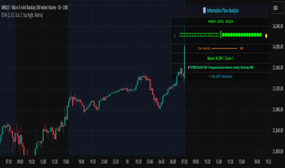
Information Flow Analysis[b🔄 Information Flow Analysis: Systematic Multi-Component Market Analysis Framework
SYSTEM OVERVIEW AND ANALYTICAL FOUNDATION
The Information Flow Kernel - Hybrid combines established technical analysis methods into a unified analytical framework. This indicator systematically processes three distinct data streams - directional price momentum, volume-weighted pressure dynamics, and intrabar development patterns - integrating them through weighted mathematical fusion to produce statistically normalized market flow measurements.
COMPREHENSIVE MATHEMATICAL FRAMEWORK
Component 1: Directional Flow Analysis
The directional component analyzes price momentum through three mathematical vectors:
Price Vector: p = C - O (intrabar directional bias)
Momentum Vector: m = C_t - C_{t-1} (bar-to-bar velocity)
Acceleration Vector: a = m_t - m_{t-1} (momentum rate of change)
Directional Signal Integration:
S_d = \text{sgn}(p) \cdot |p| + \text{sgn}(m) \cdot |m| \cdot 0.6 + \text{sgn}(a) \cdot |a| \cdot 0.3
The signum function preserves directional information while absolute values provide magnitude weighting. Coefficients create a hierarchy emphasizing intrabar movement (100%), momentum (60%), and acceleration (30%).
Final Directional Output: K_1 = S_d \cdot w_d where w_d is the directional weight parameter.
Component 2: Volume-Weighted Pressure Analysis
Volume Normalization: r_v = \frac{V_t}{\overline{V_n}} where \overline{V_n} represents the n-period simple moving average of volume.
Base Pressure Calculation: P_{base} = \Delta C \cdot r_v \cdot w_v where \Delta C = C_t - C_{t-1} and w_v is the velocity weighting factor.
Volume Confirmation Function:
f(r_v) = \begin{cases}
1.4 & \text{if } r_v > 1.2 \
0.7 & \text{if } r_v < 0.8 \
1.0 & \text{otherwise}
\end{cases}
Final Pressure Output: K_2 = P_{base} \cdot f(r_v)
Component 3: Intrabar Development Analysis
Bar Position Calculation: B = \frac{C - L}{H - L} when H - L > 0 , else B = 0.5
Development Signal Function:
S_{dev} = \begin{cases}
2(B - 0.5) & \text{if } B > 0.6 \text{ or } B < 0.4 \
0 & \text{if } 0.4 \leq B \leq 0.6
\end{cases}
Final Development Output: K_3 = S_{dev} \cdot 0.4
Master Integration and Statistical Normalization
Weighted Component Fusion: F_{raw} = 0.5K_1 + 0.35K_2 + 0.15K_3
Sensitivity Scaling: F_{master} = F_{raw} \cdot s where s is the sensitivity parameter.
Statistical Normalization Process:
Rolling Mean: \mu_F = \frac{1}{n}\sum_{i=0}^{n-1} F_{master,t-i}
Rolling Standard Deviation: \sigma_F = \sqrt{\frac{1}{n}\sum_{i=0}^{n-1} (F_{master,t-i} - \mu_F)^2}
Z-Score Computation: z = \frac{F_{master} - \mu_F}{\sigma_F}
Boundary Enforcement: z_{bounded} = \max(-3, \min(3, z))
Final Normalization: N = \frac{z_{bounded}}{3}
Flow Metrics Calculation:
Intensity: I = |z|
Strength Percentage: S = \min(100, I \times 33.33)
Extreme Detection: \text{Extreme} = I > 2.0
DETAILED INPUT PARAMETER SPECIFICATIONS
Sensitivity (0.1 - 3.0, Default: 1.0)
Global amplification multiplier applied to the master flow calculation. Functions as: F_{master} = F_{raw} \cdot s
Low Settings (0.1 - 0.5): Enhanced precision for subtle market movements. Optimal for low-volatility environments, scalping strategies, and early detection of minor directional shifts. Increases responsiveness but may amplify noise.
Moderate Settings (0.6 - 1.2): Balanced sensitivity for standard market conditions across multiple timeframes.
High Settings (1.3 - 3.0): Reduced sensitivity to minor fluctuations while emphasizing significant flow changes. Ideal for high-volatility assets, trending markets, and longer timeframes.
Directional Weighting (0.1 - 1.0, Default: 0.7)
Controls emphasis on price direction versus volume and positioning factors. Applied as: K_{1,weighted} = K_1 \times w_d
Lower Values (0.1 - 0.4): Reduces directional bias, favoring volume-confirmed moves. Optimal for ranging markets where momentum may generate false signals.
Higher Values (0.7 - 1.0): Amplifies directional signals from price vectors and acceleration. Ideal for trending conditions where directional momentum drives price action.
Velocity Weighting (0.1 - 1.0, Default: 0.6)
Scales volume-confirmed price change impact. Applied in: P_{base} = \Delta C \times r_v \times w_v
Lower Values (0.1 - 0.4): Dampens volume spike influence, focusing on sustained pressure patterns. Suitable for illiquid assets or news-sensitive markets.
Higher Values (0.8 - 1.0): Amplifies high-volume directional moves. Optimal for liquid markets where volume provides reliable confirmation.
Volume Length (3 - 20, Default: 5)
Defines lookback period for volume averaging: \overline{V_n} = \frac{1}{n}\sum_{i=0}^{n-1} V_{t-i}
Short Periods (3 - 7): Responsive to recent volume shifts, excellent for intraday analysis.
Long Periods (13 - 20): Smoother averaging, better for swing trading and higher timeframes.
DASHBOARD SYSTEM
Primary Flow Gauge
Bilaterally symmetric visualization displaying normalized flow direction and intensity:
Segment Calculation: n_{active} = \lfloor |N| \times 15 \rfloor
Left Fill: Bearish flow when N < -0.01
Right Fill: Bullish flow when N > 0.01
Neutral Display: Empty segments when |N| \leq 0.01
Visual Style Options:
Matrix: Digital blocks (▰/▱) for quantitative precision
Wave: Progressive patterns (▁▂▃▄▅▆▇█) showing flow buildup
Dots: LED-style indicators (●/○) with intensity scaling
Blocks: Modern squares (■/□) for professional appearance
Pulse: Progressive markers (⎯ to █) emphasizing intensity buildup
Flow Intensity Visualization
30-segment horizontal bar graph with mathematical fill logic:
Segment Fill: For i \in : filled if \frac{i}{29} \leq \frac{S}{100}
Color Coding System:
Orange (S > 66%): High intensity, strong directional conviction
Cyan (33% ≤ S ≤ 66%): Moderate intensity, developing bias
White (S < 33%): Low intensity, neutral conditions
Extreme Detection Indicators
Circular markers flanking the gauge with state-dependent illumination:
Activation: I > 2.0 \land |N| > 0.3
Bright Yellow: Active extreme conditions
Dim Yellow: Normal conditions
Metrics Display
Balance Value: Raw master flow output ( F_{master} ) showing absolute directional pressure
Z-Score Value: Statistical deviation ( z_{bounded} ) indicating historical context
Dynamic Narrative System
Context-sensitive interpretation based on mathematical thresholds:
Extreme Flow: I > 2.0 \land |N| > 0.6
Moderate Flow: 0.3 < |N| \leq 0.6
High Volatility: S > 50 \land |N| \leq 0.3
Neutral State: S \leq 50 \land |N| \leq 0.3
ALERT SYSTEM SPECIFICATIONS
Mathematical Trigger Conditions:
Extreme Bullish: I > 2.0 \land N > 0.6
Extreme Bearish: I > 2.0 \land N < -0.6
High Intensity: S > 80
Bullish Shift: N_t > 0.3 \land N_{t-1} \leq 0.3
Bearish Shift: N_t < -0.3 \land N_{t-1} \geq -0.3
TECHNICAL IMPLEMENTATION AND PERFORMANCE
Computational Architecture
The system employs efficient calculation methods minimizing processing overhead:
Single-pass mathematical operations for all components
Conditional visual rendering (executed only on final bar)
Optimized array operations using direct calculations
Real-Time Processing
The indicator updates continuously during bar formation, providing immediate feedback on changing market conditions. Statistical normalization ensures consistent interpretation across varying market regimes.
Market Applicability
Optimal performance in liquid markets with consistent volume patterns. May require parameter adjustment for:
Low-volume or after-hours sessions
News-driven market conditions
Highly volatile cryptocurrency markets
Ranging versus trending market environments
PRACTICAL APPLICATION FRAMEWORK
Market State Classification
This indicator functions as a comprehensive market condition assessment tool providing:
Trend Analysis: High intensity readings ( S > 66% ) with sustained directional bias indicate strong trending conditions suitable for momentum strategies.
Reversal Detection: Extreme readings ( I > 2.0 ) at key technical levels may signal potential trend exhaustion or reversal points.
Range Identification: Low intensity with neutral flow ( S < 33%, |N| < 0.3 ) suggests ranging market conditions suitable for mean reversion strategies.
Volatility Assessment: High intensity without clear directional bias indicates elevated volatility with conflicting pressures.
Integration with Trading Systems
The normalized output range facilitates integration with automated trading systems and position sizing algorithms. The statistical basis provides consistent interpretation across different market conditions and asset classes.
LIMITATIONS AND CONSIDERATIONS
This indicator combines established technical analysis methods and processes historical data without predicting future price movements. The system performs optimally in liquid markets with consistent volume patterns and may produce false signals in thin trading conditions or during news-driven market events. This indicator is provided for educational and analytical purposes only and does not constitute financial advice. Users should combine this analysis with proper risk management, position sizing, and additional confirmation methods before making any trading decisions. Past performance does not guarantee future results.
Note: The term "kernel" in this context refers to modular calculation components rather than mathematical kernel functions in the formal computational sense.
As quantitative analyst Ralph Vince noted: "The essence of successful trading lies not in predicting market direction, but in the systematic processing of market information and the disciplined management of probability distributions."
— Dskyz, Trade with insight. Trade with anticipation.
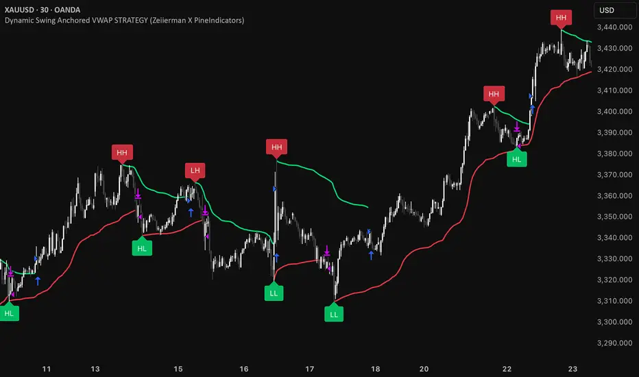
Dynamic Swing Anchored VWAP STRAT (Zeiierman/PineIndicators)Dynamic Swing Anchored VWAP STRATEGY — Zeiierman × PineIndicators (Pine Script v6)
A pivot-to-pivot Anchored VWAP strategy that adapts to volatility, enters long on bullish structure, and closes on bearish structure. Built for TradingView in Pine Script v6.
Full credits to zeiierman.
Repainting notice: The original indicator logic is repainting. Swing labels (HH/HL/LH/LL) are finalized after enough bars have printed, so labels do not occur in real time. It is not possible to execute at historical label points. Treat results as educational and validate with Bar Replay and paper trading before considering any discretionary use.
Concept
The script identifies swing highs/lows over a user-defined lookback ( Swing Period ). When structure flips (most recent swing low is newer than the most recent swing high, or vice versa), a new regime begins.
At each confirmed pivot, a fresh Anchored VWAP segment is started and updated bar-by-bar using an EWMA-style decay on price×volume and volume.
Responsiveness is controlled by Adaptive Price Tracking (APT) . Optionally, APT auto-adjusts with an ATR ratio so that high volatility accelerates responsiveness and low volatility smooths it.
Longs are opened/held in bullish regimes and closed when the regime turns bearish. No short positions are taken by design.
How it works (under the hood)
Swing detection: Uses ta.highestbars / ta.lowestbars over prd to update swing highs (ph) and lows (pl), plus their bar indices (phL, plL).
Regime logic: If phL > plL → bullish regime; else → bearish regime. A change in this condition triggers a re-anchor of the VWAP at the newest pivot.
Adaptive VWAP math: APT is converted to an exponential decay factor ( alphaFromAPT ), then applied to running sums of price×volume and volume, producing the current VWAP estimate.
Rendering: Each pivot-anchored VWAP segment is drawn as a polyline and color-coded by regime. Optional structure labels (HH/HL/LH/LL) annotate the swing character.
Orders: On bullish flips, strategy.entry("L") opens/maintains a long; on bearish flips, strategy.close("L") exits.
Inputs & controls
Swing Period (prd) — Higher values identify larger, slower swings; lower values catch more frequent pivots but add noise.
Adaptive Price Tracking (APT) — Governs the VWAP’s “half-life.” Smaller APT → faster/closer to price; larger APT → smoother/stabler.
Adapt APT by ATR ratio — When enabled, APT scales with volatility so the VWAP speeds up in turbulent markets and slows down in quiet markets.
Volatility Bias — Tunes the strength of APT’s response to volatility (above 1 = stronger effect; below 1 = milder).
Style settings — Colors for swing labels and VWAP segments, plus line width for visibility.
Trade logic summary
Entry: Long when the swing structure turns bullish (latest swing low is more recent than the last swing high).
Exit: Close the long when structure turns bearish.
Position size: qty = strategy.equity / close × 5 (dynamic sizing; scales with account equity and instrument price). Consider reducing the multiplier for a more conservative profile.
Recommended workflow
Apply to instruments with reliable volume (equities, futures, crypto; FX tick volume can work but varies by broker).
Start on your preferred timeframe. Intraday often benefits from smaller APT (more reactive); higher timeframes may prefer larger APT (smoother).
Begin with defaults ( prd=50, APT=20 ); then toggle “Adapt by ATR” and vary Volatility Bias to observe how segments tighten/loosen.
Use Bar Replay to watch how pivots confirm and how the strategy re-anchors VWAP at those confirmations.
Layer your own risk rules (stops/targets, max position cap, session filters) before any discretionary use.
Practical tips
Context filter: Consider combining with a higher-timeframe bias (e.g., daily trend) and using this strategy as an entry timing layer.
First pivot preference: Some traders prefer only the first bullish pivot after a bearish regime (and vice versa) to reduce whipsaw in choppy ranges.
Deviations: You can add VWAP deviation bands to pre-plan partial exits or re-entries on mean-reversion pulls.
Sessions: Session-based filters (RTH vs. ETH) can materially change behavior on futures and equities.
Extending the script (ideas)
Add stops/targets (e.g., ATR stop below last swing low; partial profits at k×VWAP deviation).
Introduce mirrored short logic for two-sided testing.
Include alert conditions for regime flips or for price-VWAP interactions.
Incorporate HTF confirmation (e.g., only long when daily VWAP slope ≥ 0).
Throttle entries (e.g., once per regime flip) to avoid over-trading in ranges.
Known limitations
Repainting: Swing labels and pivot confirmations depend on future bars; historical labels can look “perfect.” Treat them as annotations, not executable signals.
Execution realism: Strategy includes commission and slippage fields, yet actual fills differ by venue/liquidity.
No guarantees: Past behavior does not imply future results. This publication is for research/education only and not financial advice.
Defaults (backtest environment)
Initial capital: 10,000
Commission value: 0.01
Slippage: 1
Overlay: true
Max bars back: 5000; Max labels/polylines set for deep swing histories
Quick checklist
Add to chart and verify that the instrument has volume.
Use defaults, then tune APT and Volatility Bias with/without ATR adaptation.
Observe how each pivot re-anchors VWAP and how regime flips drive entries/exits.
Paper trade across several symbols/timeframes before any discretionary decisions.
Attribution & license
Original indicator concept and logic: Zeiierman — please credit the author.
Strategy wrapper and publication: PineIndicators .
License: CC BY-NC-SA 4.0 (Attribution-NonCommercial-ShareAlike). Respect the license when forking or publishing derivatives.
AI-Weighted RSI (Zeiierman)█ Overview
AI-Weighted RSI (Zeiierman) is an adaptive oscillator that enhances classic RSI by applying a correlation-weighted prediction layer. Instead of looking only at RSI values directly, this indicator continuously evaluates how other price- and volume-based features (returns, volatility, volume shifts) correlate with RSI, and then weights them accordingly to project the next RSI state.
The result is a smoother, forward-looking RSI framework that adapts to market conditions in real time.
By leveraging feature correlation instead of static formulas, AI-Weighted RSI behaves like a lightweight learning model, adjusting its emphasis depending on which features are most aligned with RSI behavior during the current regime.
█ How It Works
⚪ Feature Extraction
Each bar, the script computes features: log returns, RSI itself, ATR% (volatility), volume, and volume log-change.
⚪ Correlation Screening
Over a rolling learning window, it measures the correlation of each feature against RSI. The strongest relationships are ranked and selected.
⚪ Adaptive Weighting
Features are standardized (z-scored), then combined using their signed correlations as weights, building a rolling, adaptive prediction of RSI.
⚪ Prediction to RSI Weight
The predicted RSI is mapped back into a “weight” scale (±2 by default). Above 0 = bullish bias, below 0 = bearish bias, with color-graded fills to visualize overbought/oversold pressure.
⚪ Signal Line
A smoothing option (signal length) overlays a moving average of the AI-Weighted RSI for clearer trend confirmation.
█ Why AI-Weighted RSI
⚪ Adaptive to Market Regime
Because the model re-evaluates correlations continuously, it naturally shifts which features dominate, sometimes volatility explains RSI best, sometimes volume, sometimes returns.
⚪ Forward-Looking Bias
Instead of simply reflecting RSI, the model provides a projection, helping anticipate shifts in momentum before RSI itself flips.
█ How to Use
⚪ Directional Bias
Read the RSI relative to 0. Above = bullish momentum bias, below = bearish.
⚪ Overbought / Oversold Zones
Shaded fills beyond +0.5 or -0.5 highlight extremes where RSI pressure often exhausts.
⚪ Divergences
When price makes new highs/lows but AI-Weighted RSI fails to confirm, it often signals weakening momentum.
█ Settings
RSI Length: Lookback for the core RSI calculation.
Signal Length: Smoothing applied to the AI-Weighted RSI output.
Learning Window: Bars used for correlation learning and z-scoring.
-----------------
Disclaimer
The content provided in my scripts, indicators, ideas, algorithms, and systems is for educational and informational purposes only. It does not constitute financial advice, investment recommendations, or a solicitation to buy or sell any financial instruments. I will not accept liability for any loss or damage, including without limitation any loss of profit, which may arise directly or indirectly from the use of or reliance on such information.
All investments involve risk, and the past performance of a security, industry, sector, market, financial product, trading strategy, backtest, or individual's trading does not guarantee future results or returns. Investors are fully responsible for any investment decisions they make. Such decisions should be based solely on an evaluation of their financial circumstances, investment objectives, risk tolerance, and liquidity needs.

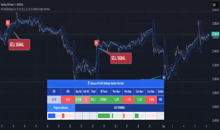
RSI ADX Bollinger Analysis High-level purpose and design philosophy
This indicator — RSI-ADX-Bollinger Analysis — is a compact, educational market-analysis toolkit that blends momentum (RSI), trend strength (ADX), volatility structure (Bollinger Bands) and simple volumetrics to provide traders a snapshot of market condition and trade idea quality. The design philosophy is explicit and layered: use each component to answer a different question about price action (momentum, conviction, volatility, participation), then combine answers to form a more robust, explainable signal. The mashup is intended for analysis and learning, not automatic execution: it surfaces the why behind signals so traders can test, learn and apply rules with risk management.
________________________________________
What each indicator contributes (component-by-component)
RSI (Relative Strength Index) — role and behavior: RSI measures short-term momentum by comparing recent gains to recent losses. A high RSI (near or above the overbought threshold) indicates strong recent buying pressure and potential exhaustion if price is extended. A low RSI (near or below the oversold threshold) indicates strong recent selling pressure and potential exhaustion or a value area for mean-reversion. In this dashboard RSI is used as the primary momentum trigger: it helps identify whether price is locally over-extended on the buy or sell side.
ADX (Average Directional Index) — role and behavior: ADX measures trend strength independently of direction. When ADX rises above a chosen threshold (e.g., 25), it signals that the market is trending with conviction; ADX below the threshold suggests range or weak trend. Because patterns and momentum signals perform differently in trending vs. ranging markets, ADX is used here as a filter: only when ADX indicates sufficient directional strength does the system treat RSI+BB breakouts as meaningful trade candidates.
Bollinger Bands — role and behavior: Bollinger Bands (20-period basis ± N standard deviations) show volatility envelope and relative price position vs. a volatility-adjusted mean. Price outside the upper band suggests pronounced extension relative to recent volatility; price outside the lower band suggests extended weakness. A band expansion (increasing width) signals volatility breakout potential; contraction signals range-bound conditions and potential squeeze. In this dashboard, Bollinger Bands provide the volatility/structural context: RSI extremes plus price beyond the band imply a stronger, volatility-backed move.
Volume split & basic MA trend — role and behavior: Buy-like and sell-like volume (simple heuristic using close>open or closeopen) or sell-like (close1.2 for validation and compare win rate and expectancy.
4. TF alignment: Accept signals only when higher timeframe (e.g., 4h) trend agrees — compare results.
5. Parameter sensitivity: Vary RSI threshold (70/30 vs 80/20), Bollinger stddev (2 vs 2.5), and ADX threshold (25 vs 30) and measure stability of results.
These exercises teach both statistical thinking and the specific failure modes of the mashup.
________________________________________
Limitations, failure modes and caveats (explicit & teachable)
• ADX and Bollinger measures lag during fast-moving news events — signals can be late or wrong during earnings, macro shocks, or illiquid sessions.
• Volume classification by open/close is a heuristic; it does not equal TAPEDATA, footprint or signed volume. Use it as supportive evidence, not definitive proof.
• RSI can remain overbought or oversold for extended stretches in persistent trends — relying solely on RSI extremes without ADX or BB context invites large drawdowns.
• Small-cap or low-liquidity instruments yield noisy band behavior and unreliable volume ratios.
Being explicit about these limitations is a strong point in a TradingView description — it demonstrates transparency and educational intent.
________________________________________
Originality & mashup justification (text you can paste)
This script intentionally combines classical momentum (RSI), volatility envelope (Bollinger Bands) and trend-strength (ADX) because each indicator answers a different and complementary question: RSI answers is price locally extreme?, Bollinger answers is price outside normal volatility?, and ADX answers is the market moving with conviction?. Volume participation then acts as a practical check for real market involvement. This combination is not a simple “indicator mashup”; it is a designed ensemble where each element reduces the others’ failure modes and together produce a teachable, testable signal framework. The script’s purpose is educational and analytical — to show traders how to interpret the interplay of momentum, volatility, and trend strength.
________________________________________
TradingView publication guidance & compliance checklist
To satisfy TradingView rules about mashups and descriptions, include the following items in your script description (without exposing source code):
1. Purpose statement: One or two lines describing the script’s objective (educational multi-indicator market overview and idea filter).
2. Component list: Name the major modules (RSI, Bollinger Bands, ADX, volume heuristic, SMA trend checks, signal tracking) and one-sentence reason for each.
3. How they interact: A succinct non-code explanation: “RSI finds momentum extremes; Bollinger confirms volatility expansion; ADX confirms trend strength; all three must align for a BUY/SELL.”
4. Inputs: List adjustable inputs (RSI length and thresholds, BB length & stddev, ADX threshold & smoothing, volume MA, table position/size).
5. Usage instructions: Short workflow (check TF alignment → confirm participation → define stop & R:R → backtest).
6. Limitations & assumptions: Explicitly state volume is approximated, ADX has lag, and avoid promising guaranteed profits.
7. Non-promotional language: No external contact info, ads, claims of exclusivity or guaranteed outcomes.
8. Trademark clause: If you used trademark symbols, remove or provide registration proof.
9. Risk disclaimer: Add the copy-ready disclaimer below.
This matches TradingView’s request for meaningful descriptions that explain originality and inter-component reasoning.
________________________________________
Copy-ready short publication description (paste into TradingView)
Advanced RSI-ADX-Bollinger Market Overview — educational multi-indicator dashboard. This script combines RSI (momentum extremes), Bollinger Bands (volatility envelope and band expansion), ADX (trend strength), simple SMA trend bias and a basic buy/sell volume heuristic to surface high-quality idea candidates. Signals require alignment of momentum, volatility expansion and rising ADX; volume participation is displayed to support signal confidence. Inputs are configurable (RSI length/levels, BB length/stddev, ADX length/threshold, volume MA, display options). This tool is intended for analysis and learning — not for automated execution. Users should back test and apply robust risk management. Limitations: volume classification here is a heuristic (close>open), ADX and BB measures lag in fast news events, and results vary by instrument liquidity.
________________________________________
Copy-ready risk & misuse disclaimer (paste into description or help file)
This script is provided for educational and analytical purposes only and does not constitute financial or investment advice. It does not guarantee profits. Indicators are heuristics and may give false or late signals; always back test and paper-trade before using real capital. The author is not responsible for trading losses resulting from the use or misuse of this indicator. Use proper position sizing and risk controls.
________________________________________
Risk Disclaimer: This tool is provided for education and analysis only. It is not financial advice and does not guarantee returns. Users assume all risk for trades made based on this script. Back test thoroughly and use proper risk management.
Primitive Delta DivergencePrimitive Delta Divergence
This indicator detects volume-price divergences by analyzing the relationship between price direction and volume bias over a rolling lookback period, revealing potential momentum shifts before they become apparent in price action alone.
Instead of relying solely on price movements, you can identify moments when volume sentiment contradicts price direction — a core concept borrowed from footprint chart analysis, adapted for traditional bar charts.
For example, when price moves higher but volume is predominantly bearish, or when price declines while volume shows bullish accumulation.
🔹 How it works
Lookback Period (n) → defines the rolling window for analyzing price and volume relationships
Creates a "meta-candle" from the lookback period, comparing its open vs. close for price bias
Volume classification → separates each bar's volume into bullish (green candles), bearish (red candles), or neutral (doji candles)
Volume bias calculation → generates a continuous score (-1 to +1) representing the directional volume pressure
Plots divergence signals when price direction and volume bias disagree
🔹 Use cases
Spot early momentum exhaustion when price and volume move in opposite directions
Identify potential reversal zones where volume suggests underlying weakness or strength
Enhance entry/exit timing by incorporating volume-based confirmation alongside price action
Apply footprint-style analysis to any timeframe without specialized charting tools
✨ Primitive Delta Divergence reveals the hidden story volume tells about price, uncovering divergences that traditional indicators might miss.
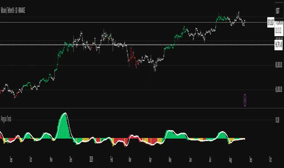
Penguin Trend with RSI on DiffVisualizes volatility regime via the percent spread between the upper Bollinger Band and the upper Keltner Channel, with bar colors from a lightweight trend engine and an RSI computed on the Diff signal. Supports SMA/EMA/WMA/RMA/HMA/VWMA/VWAP and an optional calculation timeframe. Defaults preserve the original look and behavior.
Penguin Trend with RSI on Diff shows expansion vs. compression in price action by comparing two classic volatility envelopes. It computes:
Diff% = (UpperBB − UpperKC) / UpperKC × 100
• Diff > 0: Bollinger Bands are wider than Keltner Channels → expansion / momentum regime
• Diff < 0: BB narrower than KC → compression / squeeze regime
A white “Average Diff” line smooths Diff% (default: SMA(5)) to highlight regime shifts. Bars are colored only when Diff > 0 to focus on expansion phases. A lightweight trend engine defines four states from a fast/slow MA bias and a short “thrust” MA on ohlc4:
• Green: Bullish bias and thrust > fast MA (healthy upside thrust)
• Red: Bearish bias and thrust < fast MA (healthy downside thrust)
• Yellow: Bullish bias but thrust ≤ fast MA (pullback/weakness)
• Blue: Bearish bias but thrust ≥ fast MA (bear rally/short squeeze)
RSI on Diff:
The indicator adds an RSI applied to Diff% to gauge momentum of the expansion/compression signal itself. Choose between Built-in RSI or a manual RMA-based computation, and optionally smooth it. Default OB/OS lines are 70/30.
How it works:
• Bollinger Bands (BB): Basis = selected MA of src (default SMA(20)); Width = StdDev × Mult (default 2.0)
• Keltner Channels (KC): Basis = selected MA of src (default SMA(20)); Width = ATR(kcATR) × Mult (defaults 20 and 2.0)
• Diff%: Safe division guards against division-by-zero
• MA engine: Select SMA / EMA / WMA / RMA / HMA / VWMA / VWAP for BB/KC bases, Average Diff, and trend components (VWAP is session-anchored)
• Calculation timeframe: Compute internals on a chosen TF via request.security() while viewing any chart TF
Inputs (key):
• Calculation timeframe: Empty = chart TF; set e.g., 60/240 to compute on that TF
• BB: Length, StdDev Mult, MA Type
• KC: Basis Length, ATR Length, Multiplier, MA Type
• Average Diff: Length and MA Type
• RSI on Diff: RSI Length, Method (Built-in or Manual RMA), Smoothing Length, OB/OS levels, show/hide
• Trend Engine: Fast/Slow lengths & MA type, Signal (kept for completeness), Thrust MA length & type
• Display/Visibility: Paint bars only when Diff > 0; show zero line; “true Blue” color toggle; show/hide Diff columns and Average Diff
How to use:
1. Regime changes: Watch Diff% or Average Diff crossing 0. Above zero favors momentum/continuation setups; below zero suggests compression and potential breakout conditions.
2. State confirmation: During expansion (Diff > 0), prioritize Green/Red for aligned thrust; treat Yellow/Blue as cautionary/contrarian.
3. RSI on Diff: Use OB/OS and crossovers for timing entries/exits or for confirming/negating expansion strength.
Alerts:
• Diff crosses above/below 0
• Average Diff crosses above/below 0
• RSI(Diff) crosses above OB / below OS
• State changes: GREEN / RED / YELLOW / BLUE
Notes & limitations:
• VWAP is session-anchored and best on intraday data. If not applicable on the selected calculation TF, the script automatically falls back to EMA.
• Defaults (SMA(20) for BB/KC, multipliers 2.0, SMA(5) Average Diff, original trend coloring and bar painting) preserve the original appearance.
• RSI on Diff is plotted in the same pane for a compact workflow; you can hide it or split into a separate indicator if desired.
Release notes:
v6.0 — Upgraded to Pine v6. Added multi-MA options (SMA/EMA/WMA/RMA/HMA/VWMA/VWAP), calculation timeframe, RSI on Diff (Built-in or Manual RMA) with smoothing, safe division guard, optional zero line, and optional true Blue color. Defaults retain the original behavior.
License / disclaimer:
© waranyu.trkm — MIT License. Educational use only; not financial advice.

Penguin TrendMeasures the volatility regime by comparing the upper Bollinger Band to the upper Keltner Channel and colors bars with a lightweight trend state. Supports SMA/EMA/WMA/RMA/HMA/VWMA/VWAP and a selectable calculation timeframe. Default settings preserve the original look and behavior.
Penguin Trend visualizes expansion vs. compression in price action by comparing two classic volatility envelopes. It computes:
Diff% = (UpperBB − UpperKC) / UpperKC × 100
* Diff > 0: Bollinger Bands are wider than Keltner Channels -> expansion / momentum regime.
* Diff < 0: BB narrower than KC -> compression / squeeze regime.
A white “Average Difference” line smooths Diff% (default: SMA(5)) to help spot regime shifts.
Trend coloring (kept from original):
Bars are colored only when Diff > 0 to emphasize expansion phases. A lightweight trend engine defines four states using a fast/slow MA bias and a short “thrust” MA applied to ohlc4:
* Green: Bullish bias and thrust > fast MA (healthy upside thrust).
* Red: Bearish bias and thrust < fast MA (healthy downside thrust).
* Yellow: Bullish bias but thrust ≤ fast MA (pullback/weakness).
* Blue: Bearish bias but thrust ≥ fast MA (bear rally/short squeeze).
Note: By default, Blue renders as Yellow to preserve the original visual style. Enable “Use true BLUE color” if you prefer Aqua for Blue.
How it works (under the hood):
* Bollinger Bands (BB): Basis = selected MA of src (default SMA(20)). Width = StdDev × Mult (default 2.0).
* Keltner Channels (KC): Basis = selected MA of src (default SMA(20)). Width = ATR(kcATR) × Mult (defaults 20 and 2.0).
* Diff%: Safe division guards against division-by-zero.
* MA engine: You can choose SMA / EMA / WMA / RMA / HMA / VWMA / VWAP for BB/KC bases, Diff smoothing, and the trend components (VWAP is session-anchored).
* Calculation timeframe: Set “Calculation timeframe” to compute all internals on a chosen TF via request.security() while viewing any chart TF.
Inputs (key ones):
* Calculation timeframe: Empty = use chart TF; if set (e.g., 60), all internals compute on that TF.
* BB: Length, StdDev Mult, MA Type.
* KC: Basis Length, ATR Length, Multiplier, MA Type.
* Smoothing: Average Length & MA Type for the “Average Difference” line.
* Trend Engine: Fast/Slow lengths & MA type; Signal (kept for completeness); Thrust length & MA type (defaults replicate original behavior).
* Display: Paint bars only when Diff > 0; optional Zero line; optional true Blue color.
How to use:
1. Regime changes: Watch Diff% or Average Diff crossing 0. Above zero favors momentum/continuation setups; below zero suggests compression and potential breakout conditions.
2. State confirmation: Use bar colors to qualify expansion: Green/Red indicate expansion aligned with trend thrust; Yellow/Blue flag weaker/contrarian thrust during expansion.
3. Multi-timeframe analysis: Run calculations on a higher TF (e.g., H1/H4) while trading a lower TF chart to smooth noise.
Alerts:
* Diff crosses above/below 0.
* Average Diff crosses above/below 0.
* State changes: GREEN / RED / YELLOW / BLUE.
Notes & limitations:
* VWAP is session-anchored and best on intraday data. If not applicable on the selected calculation TF, the script automatically falls back to EMA.
* Default parameters (SMA(20) for BB/KC, multipliers 2.0, SMA(5) smoothing, trend logic and bar painting) preserve the original appearance.
Release notes:
v6.0 — Rewritten in Pine v6 with structured inputs and guards. Multi-MA support (SMA/EMA/WMA/RMA/HMA/VWMA/VWAP). Calculation timeframe via request.security() for multi-TF workflows. Safe division; optional zero line; optional true Blue color. Original visuals and behavior preserved by default.
License / disclaimer:
© waranyu.trkm — MIT License. Educational use only; not financial advice.
Scalping Line Strategy📌 Scalping Line Strategy – A Precision Crossover System
🔎 Overview
The Scalping Line Strategy is a short-term trading system built around the concept of momentum-driven crossovers between a smoothed moving average filter and a fast signal line. It is designed for scalpers and intraday traders who seek clear entry signals, minimal lag, and adaptive filtering to fit volatile market conditions.
At its core, the strategy uses a custom signal line ("Scalping Line"), which is derived from the difference between a double-smoothed moving average and a shorter-period signal line. Trade entries are triggered when this Scalping Line crosses above or below zero, providing a clean and rules-based framework for both long and short setups.
⚙️ Core Logic
Main Trend Filter – A double-smoothed moving average is calculated over a configurable period (default 100). This reduces noise and provides a more robust backbone for scalping signals.
Percent-Based Filter – To avoid false signals, a customizable percentage filter adjusts how closely the system “respects” price deviations from the moving average. This helps filter out insignificant fluctuations.
Signal Line – A shorter-period simple moving average (default 7) provides faster responsiveness to recent price action.
Scalping Line (SLI) – Calculated as the difference between the fast signal line and the smoothed moving average. When the SLI crosses zero, it signals a potential momentum shift.
SLI > 0 → Momentum bias is bullish.
SLI < 0 → Momentum bias is bearish.
🎯 Trade Direction & Flexibility
Trade Direction Control:
Choose between Long Only, Short Only, or Both to tailor the system to your trading style.
Signal Flip Option:
By default, long entries occur when the SLI crosses below zero, and shorts when it crosses above zero. This orientation can be flipped, allowing for alternative interpretations of the signals depending on how you want to capture momentum in your market.
🕒 Time Window Filtering
For intraday traders, a time filter can be enabled to restrict signals to specific trading sessions (e.g., 9 AM – 4 PM EST). This is particularly useful when trading assets such as equities or futures that have strong intraday volatility windows.
📈 Visuals & Clarity
Scalping Line Plot: Displayed as a dynamic oscillator around a zero baseline.
Histogram Fill: Green when above zero (bullish bias), red when below zero (bearish bias).
Signal Markers: Clear arrows mark long and short entries at crossover points.
Zero Line Reference: A flat gray line at zero assists in visually gauging momentum shifts.
🚀 Strategy Execution
Long Entry: Triggered when SLI crosses below zero (or above zero if flip is enabled) within allowed session hours.
Short Entry: Triggered when SLI crosses above zero (or below zero if flip is enabled) within allowed session hours.
Built-in Signal Cancels: Pending entries are canceled if conditions are no longer valid, ensuring no stale trades remain active.
✅ Best Use Cases
Markets: Works across equities, forex, crypto, and futures with sufficient intraday volatility.
Timeframes: Most effective on 1m to 15m charts for scalping setups, but adaptable to higher frames for swing trading.
Style: Traders who appreciate simple, rules-based momentum crossovers will find this system easy to follow and highly adaptable.
⚠️ Risk Management Note
This strategy is strictly an entry signal framework. Position sizing, stop-loss, and take-profit rules must be overlaid based on your risk management style. Always validate results with backtesting and forward testing before applying to live trading accounts.
📜 Final Thoughts
The Scalping Line Strategy offers a refined, easy-to-interpret approach to intraday trading. By combining smoothed moving averages, adaptive filtering, and flexible signal options, it helps traders identify short-term momentum shifts with clarity and confidence, making it a highly configurable tool for scalping-focused strategies.

VWAP For Loop [BackQuant]VWAP For Loop
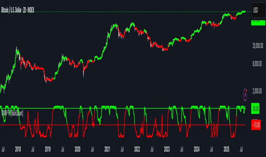
What this tool does—in one sentence
A volume-weighted trend gauge that anchors VWAP to a calendar period (day/week/month/quarter/year) and then scores the persistence of that VWAP trend with a simple for-loop “breadth” count; the result is a clean, threshold-driven oscillator plus an optional VWAP overlay and alerts.
Plain-English overview
Instead of judging raw price alone, this indicator focuses on anchored VWAP —the market’s average price paid during your chosen institutional period. It then asks a simple question across a configurable set of lookback steps: “Is the current anchored VWAP higher than it was i bars ago—or lower?” Each “yes” adds +1, each “no” adds −1. Summing those answers creates a score that reflects how consistently the volume-weighted trend has been rising or falling. Extreme positive scores imply persistent, broad strength; deeply negative scores imply persistent weakness. Crossing predefined thresholds produces objective long/short events and color-coded context.
Under the hood
• Anchoring — VWAP using hlc3 × volume resets exactly when the selected period rolls:
Day → session change, Week → new week, Month → new month, Quarter/Year → calendar quarter/year.
• For-loop scoring — For lag steps i = , compare today’s VWAP to VWAP .
– If VWAP > VWAP , add +1.
– Else, add −1.
The final score ∈ , where N = (end − start + 1). With defaults (1→45), N = 45.
• Signal logic (stateful)
– Long when score > upper (e.g., > 40 with N = 45 → VWAP higher than ~89% of checked lags).
– Short on crossunder of lower (e.g., dropping below −10).
– A compact state variable ( out ) holds the current regime: +1 (long), −1 (short), otherwise unchanged. This “stickiness” avoids constant flipping between bars without sufficient evidence.
Why VWAP + a breadth score?
• VWAP aggregates both price and volume—where participants actually traded.
• The breadth-style count rewards consistency of the anchored trend, not one-off spikes.
• Thresholds give you binary structure when you need it (alerts, automation), without complex math.
What you’ll see on the chart
• Sub-pane oscillator — The for-loop score line, colored by regime (long/short/neutral).
• Main-pane VWAP (optional) — Even though the indicator runs off-chart, the anchored VWAP can be overlaid on price (toggle visibility and whether it inherits trend colors).
• Threshold guides — Horizontal lines for the long/short bands (toggle).
• Cosmetics — Optional candle painting and background shading by regime; adjustable line width and colors.
Input map (quick reference)
• VWAP Anchor Period — Day, Week, Month, Quarter, Year.
• Calculation Start/End — The for-loop lag window . With 1→45, you evaluate 45 comparisons.
• Long/Short Thresholds — Default upper=40, lower=−10 (asymmetric by design; see below).
• UI/Style — Show thresholds, paint candles, background color, line width, VWAP visibility and coloring, custom long/short colors.
Interpreting the score
• Near +N — Current anchored VWAP is above most historical VWAP checkpoints in the window → entrenched strength.
• Near −N — Current anchored VWAP is below most checkpoints → entrenched weakness.
• Between — Mixed, choppy, or transitioning regimes; use thresholds to avoid reacting to noise.
Why the asymmetric default thresholds?
• Long = score > upper (40) — Demands unusually broad upside persistence before declaring “long regime.”
• Short = crossunder lower (−10) — Triggers only on downward momentum events (a fresh breach), not merely being below −10. This combination tends to:
– Capture sustained uptrends only when they’re very strong.
– Flag downside turns as they occur, rather than waiting for an extreme negative breadth.
Tuning guide
Choose an anchor that matches your horizon
– Intraday scalps : Day anchor on intraday charts.
– Swing/position : Month or Quarter anchor on 1h/4h/D charts to capture institutional cycles.
Pick the for-loop window
– Larger N (bigger end) = stronger evidence requirement, smoother oscillator.
– Smaller N = faster, more reactive score.
Set achievable thresholds
– Ensure upper ≤ N and lower ≥ −N ; if N=30, an upper of 40 can never trigger.
– Symmetric setups (e.g., +20/−20) are fine if you want balanced behavior.
Match visuals to intent
– Enabling VWAP coloring lets you see regime directly on price.
– Background shading is useful for discretionary reading; turn it off for cleaner automation displays.
Playbook examples
• Trend confirmation with disciplined entries — On Month anchor, N=45, upper=38–42: when the long regime engages, use pullbacks toward anchored VWAP on the main pane for entries, with stops just beyond VWAP or a recent swing.
• Downside transition detection — Keep lower around −8…−12 and watch for crossunders; combine with price losing anchored VWAP to validate risk-off.
• Intraday bias filter — Day anchor on a 5–15m chart, N=20–30, upper ~ 16–20, lower ~ −6…−10. Only take longs while score is positive and above a midline you define (e.g., 0), and shorts only after a genuine crossunder.
Behavior around resets (important)
Anchored VWAP is hard-reset each period. Immediately after a reset, the series can be young and comparisons to pre-reset values may span two periods. If you prefer within-period evaluation only, choose end small enough not to bridge typical period length on your timeframe, or accept that the breadth test intentionally spans regimes.
Alerts included
• VWAP FL Long — Fires when the long condition is true (score > upper and not in short).
• VWAP FL Short — Fires on crossunder of the lower threshold (event-driven).
Messages include {{ticker}} and {{interval}} placeholders for routing.
Strengths
• Simple, transparent math — Easy to reason about and validate.
• Volume-aware by construction — Decisions reference VWAP, not just price.
• Robust to single-bar noise — Needs many lags to agree before flipping state (by design, via thresholds and the stateful output).
Limitations & cautions
• Threshold feasibility — If N < upper or |lower| > N, signals will never trigger; always cross-check N.
• Path dependence — The state variable persists until a new event; if you want frequent re-evaluation, lower thresholds or reduce N.
• Regime changes — Calendar resets can produce early ambiguity; expect a few bars for the breadth to mature.
• VWAP sensitivity to volume spikes — Large prints can tilt VWAP abruptly; that behavior is intentional in VWAP-based logic.
Suggested starting profiles
• Intraday trend bias : Anchor=Day, N=25 (1→25), upper=18–20, lower=−8, paint candles ON.
• Swing bias : Anchor=Month, N=45 (1→45), upper=38–42, lower=−10, VWAP coloring ON, background OFF.
• Balanced reactivity : Anchor=Week, N=30 (1→30), upper=20–22, lower=−10…−12, symmetric if desired.
Implementation notes
• The indicator runs in a separate pane (oscillator), but VWAP itself is drawn on price using forced overlay so you can see interactions (touches, reclaim/loss).
• HLC3 is used for VWAP price; that’s a common choice to dampen wick noise while still reflecting intrabar range.
• For-loop cap is kept modest (≤50) for performance and clarity.
How to use this responsibly
Treat the oscillator as a bias and persistence meter . Combine it with your entry framework (structure breaks, liquidity zones, higher-timeframe context) and risk controls. The design emphasizes clarity over complexity—its edge is in how strictly it demands agreement before declaring a regime, not in predicting specific turns.
Summary
VWAP For Loop distills the question “How broadly is the anchored, volume-weighted trend advancing or retreating?” into a single, thresholded score you can read at a glance, alert on, and color through your chart. With careful anchoring and thresholds sized to your window length, it becomes a pragmatic bias filter for both systematic and discretionary workflows.
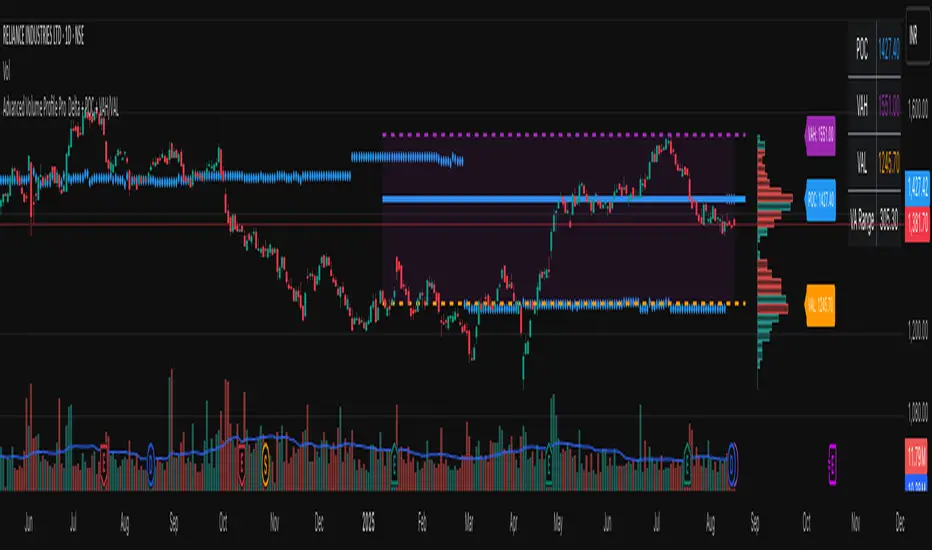
Advanced Volume Profile Pro Delta + POC + VAH/VAL# Advanced Volume Profile Pro - Delta + POC + VAH/VAL Analysis System
## WHAT THIS SCRIPT DOES
This script creates a comprehensive volume profile analysis system that combines traditional volume-at-price distribution with delta volume calculations, Point of Control (POC) identification, and Value Area (VAH/VAL) analysis. Unlike standard volume indicators that show only total volume over time, this script analyzes volume distribution across price levels and estimates buying vs selling pressure using multiple calculation methods to provide deeper market structure insights.
## WHY THIS COMBINATION IS ORIGINAL AND USEFUL
**The Problem Solved:** Traditional volume indicators show when volume occurs but not where price finds acceptance or rejection. Standalone volume profiles lack directional bias information, while basic delta calculations don't provide structural context. Traders need to understand both volume distribution AND directional sentiment at key price levels.
**The Solution:** This script implements an integrated approach that:
- Maps volume distribution across price levels using configurable row density
- Estimates delta (buying vs selling pressure) using three different methodologies
- Identifies Point of Control (highest volume price level) for key support/resistance
- Calculates Value Area boundaries where 70% of volume traded
- Provides real-time alerts for key level interactions and volume imbalances
**Unique Features:**
1. **Developing POC Visualization**: Real-time tracking of Point of Control migration throughout the session via blue dotted trail, revealing institutional accumulation/distribution patterns before they complete
2. **Multi-Method Delta Calculation**: Price Action-based, Bid/Ask estimation, and Cumulative methods for different market conditions
3. **Adaptive Timeframe System**: Auto-adjusts calculation parameters based on chart timeframe for optimal performance
4. **Flexible Profile Types**: N Bars Back (precise control), Days Back (calendar-based), and Session-based analysis modes
5. **Advanced Imbalance Detection**: Identifies and highlights significant buying/selling imbalances with configurable thresholds
6. **Comprehensive Alert System**: Monitors POC touches, Value Area entry/exit, and major volume imbalances
## HOW THE SCRIPT WORKS TECHNICALLY
### Core Volume Profile Methodology:
**1. Price Level Distribution:**
- Divides price range into user-defined rows (10-50 configurable)
- Calculates row height: `(Highest Price - Lowest Price) / Number of Rows`
- Distributes each bar's volume across price levels it touched proportionally
**2. Delta Volume Calculation Methods:**
**Price Action Method:**
```
Price Range = High - Low
Buy Pressure = (Close - Low) / Price Range
Sell Pressure = (High - Close) / Price Range
Buy Volume = Total Volume × Buy Pressure
Sell Volume = Total Volume × Sell Pressure
Delta = Buy Volume - Sell Volume
```
**Bid/Ask Estimation Method:**
```
Average Price = (High + Low + Close) / 3
Buy Volume = Close > Average ? Volume × 0.6 : Volume × 0.4
Sell Volume = Total Volume - Buy Volume
```
**Cumulative Method:**
```
Buy Volume = Close > Open ? Volume : Volume × 0.3
Sell Volume = Close ≤ Open ? Volume : Volume × 0.3
```
**3. Point of Control (POC) Identification:**
- Scans all price levels to find maximum volume concentration
- POC represents the price level with highest trading activity
- Acts as significant support/resistance level
- **Developing POC Feature**: Tracks POC evolution in real-time via blue dotted trail, showing how institutional interest migrates throughout the session. Upward POC migration indicates accumulation patterns, downward migration suggests distribution, providing early trend signals before price confirmation.
**4. Value Area Calculation:**
- Starts from POC and expands up/down to encompass 70% of total volume
- VAH (Value Area High): Upper boundary of value area
- VAL (Value Area Low): Lower boundary of value area
- Expansion algorithm prioritizes direction with higher volume
**5. Adaptive Range Selection:**
Based on profile type and timeframe optimization:
- **N Bars Back**: Fixed lookback period with performance optimization (20-500 bars)
- **Days Back**: Calendar-based analysis with automatic timeframe adjustment (1-365 days)
- **Session**: Current trading session or custom session times
### Performance Optimization Features:
- **Sampling Algorithm**: Reduces calculation load on large datasets while maintaining accuracy
- **Memory Management**: Clears previous drawings to prevent performance degradation
- **Safety Constraints**: Prevents excessive memory usage with configurable limits
## HOW TO USE THIS SCRIPT
### Initial Setup:
1. **Profile Configuration**: Select profile type based on trading style:
- N Bars Back: Precise control over data range
- Days Back: Intuitive calendar-based analysis
- Session: Real-time session development
2. **Row Density**: Set number of rows (30 default) - more rows = higher resolution, slower performance
3. **Delta Method**: Choose calculation method based on market type:
- Price Action: Best for trending markets
- Bid/Ask Estimate: Good for ranging markets
- Cumulative: Smoothed approach for volatile markets
4. **Visual Settings**: Configure colors, position (left/right), and display options
### Reading the Profile:
**Volume Bars:**
- **Length**: Represents relative volume at that price level
- **Color**: Green = net buying pressure, Red = net selling pressure
- **Intensity**: Darker colors indicate volume imbalances above threshold
**Key Levels:**
- **POC (Blue Line)**: Highest volume price - major support/resistance
- **VAH (Purple Dashed)**: Value Area High - upper boundary of fair value
- **VAL (Orange Dashed)**: Value Area Low - lower boundary of fair value
- **Value Area Fill**: Shaded region showing main trading range
**Developing POC Trail:**
- **Blue Dotted Lines**: Show real-time POC evolution throughout the session
- **Migration Patterns**: Upward trail indicates bullish accumulation, downward trail suggests bearish distribution
- **Early Signals**: POC movement often precedes price movement, providing advance warning of institutional activity
- **Institutional Footprints**: Reveals where smart money concentrated volume before final POC establishment
### Trading Applications:
**Support/Resistance Analysis:**
- POC acts as magnetic price level - expect reactions
- VAH/VAL provide intermediate support/resistance levels
- Profile edges show areas of low volume acceptance
**Developing POC Analysis:**
- **Upward Migration**: POC moving higher = institutional accumulation, bullish bias
- **Downward Migration**: POC moving lower = institutional distribution, bearish bias
- **Stable POC**: Tight clustering = balanced market, range-bound conditions
- **Early Trend Detection**: POC direction change often precedes price breakouts
**Entry Strategies:**
- Buy at VAL with POC as target (in uptrends)
- Sell at VAH with POC as target (in downtrends)
- Breakout plays above/below profile extremes
**Volume Imbalance Trading:**
- Strong buying imbalance (>60% threshold) suggests continued upward pressure
- Strong selling imbalance suggests continued downward pressure
- Imbalances near key levels provide high-probability setups
**Multi-Timeframe Context:**
- Use higher timeframe profiles for major levels
- Lower timeframe profiles for precise entries
- Session profiles for intraday trading structure
## SCRIPT SETTINGS EXPLANATION
### Volume Profile Settings:
- **Profile Type**: Determines data range for calculation
- N Bars Back: Exact number of bars (20-500 range)
- Days Back: Calendar days with timeframe adaptation (1-365 days)
- Session: Trading session-based (intraday focus)
- **Number of Rows**: Profile resolution (10-50 range)
- **Profile Width**: Visual width as chart percentage (10-50%)
- **Value Area %**: Volume percentage for VA calculation (50-90%, 70% standard)
- **Auto-Adjust**: Automatically optimizes for different timeframes
### Delta Volume Settings:
- **Show Delta Volume**: Enable/disable delta calculations
- **Delta Calculation Method**: Choose methodology based on market conditions
- **Highlight Imbalances**: Visual emphasis for significant volume imbalances
- **Imbalance Threshold**: Percentage for imbalance detection (50-90%)
### Session Settings:
- **Session Type**: Daily, Weekly, Monthly, or Custom periods
- **Custom Session Time**: Define specific trading hours
- **Previous Sessions**: Number of historical sessions to display
### Days Back Settings:
- **Lookback Days**: Number of calendar days to analyze (1-365)
- **Automatic Calculation**: Script automatically converts days to bars based on timeframe:
- Intraday: Accounts for 6.5 trading hours per day
- Daily: 1 bar per day
- Weekly/Monthly: Proportional adjustment
### N Bars Back Settings:
- **Lookback Bars**: Exact number of bars to analyze (20-500)
- **Precise Control**: Best for systematic analysis and backtesting
### Visual Customization:
- **Colors**: Bullish (green), Bearish (red), and level colors
- **Profile Position**: Left or Right side of chart
- **Profile Offset**: Distance from current price action
- **Labels**: Show/hide level labels and values
- **Smooth Profile Bars**: Enhanced visual appearance
### Alert Configuration:
- **POC Touch**: Alerts when price interacts with Point of Control
- **VA Entry/Exit**: Alerts for Value Area boundary interactions
- **Major Imbalance**: Alerts for significant volume imbalances
## VISUAL FEATURES
### Profile Display:
- **Horizontal Bars**: Volume distribution across price levels
- **Color Coding**: Delta-based coloring for directional bias
- **Smooth Rendering**: Optional smoothing for cleaner appearance
- **Transparency**: Configurable opacity for chart readability
### Level Lines:
- **POC**: Solid blue line with optional label
- **VAH/VAL**: Dashed colored lines with value displays
- **Extension**: Lines extend across relevant time periods
- **Value Area Fill**: Optional shaded region between VAH/VAL
### Information Table:
- **Current Values**: Real-time POC, VAH, VAL prices
- **VA Range**: Value Area width calculation
- **Positioning**: Multiple table positions available
- **Text Sizing**: Adjustable for different screen sizes
## IMPORTANT USAGE NOTES
**Realistic Expectations:**
- Volume profile analysis provides structural context, not trading signals
- Delta calculations are estimations based on price action, not actual order flow
- Past volume distribution does not guarantee future price behavior
- Combine with other analysis methods for comprehensive market view
**Best Practices:**
- Use appropriate profile types for your trading style:
- Day Trading: Session or Days Back (1-5 days)
- Swing Trading: Days Back (10-30 days) or N Bars Back
- Position Trading: Days Back (60-180 days)
- Consider market context (trending vs ranging conditions)
- Verify key levels with additional technical analysis
- Monitor profile development for changing market structure
**Performance Considerations:**
- Higher row counts increase calculation complexity
- Large lookback periods may affect chart performance
- Auto-adjust feature optimizes for most use cases
- Consider using session profiles for intraday efficiency
**Limitations:**
- Delta calculations are estimations, not actual transaction data
- Profile accuracy depends on available price/volume history
- Effectiveness varies across different instruments and market conditions
- Requires understanding of volume profile concepts for optimal use
**Data Requirements:**
- Requires volume data for accurate calculations
- Works best on liquid instruments with consistent volume
- May be less effective on very low volume or exotic instruments
This script serves as a comprehensive volume analysis tool for traders who need detailed market structure information with integrated directional bias analysis and real-time POC development tracking for informed trading decisions.
ABS Companion Oscillator — Trend / Exhaustion / New Trend (v1.1)
# ABS Companion Oscillator — Trend / Exhaustion / New Trend (v1.1)
## What it is (quick take)
**ABS CO** is a unified **–100…+100 trend oscillator** that fuses:
* **Regime**: EMA stack (fast/slow/long) + **HTF slope** (e.g., 60-minute)
* **Momentum**: **TSI** vs its signal
* **Stretch**: session-anchored **VWAP Z-score** for exhaustion and “fresh-trend” sanity checks
It paints the oscillator with **lime** in upstate, **red** in downstate, **gray** in neutral, and tags:
* **NEW↑ / NEW↓** when a **new trend** likely starts (zero-line cross with acceptable stretch)
* **EXH↑ / EXH↓** when an **existing trend looks exhausted** (large |Z| + momentum rollback)
> Use it as a **direction filter and context layer**. Works great in front of an entry engine and behind an exit tool.
---
## How to use it (operational workflow)
1. **Read the state**
* **Uptrend** when the oscillator is **≥ upThresh** (default +55) → prefer **long-side** plays.
* **Downtrend** when the oscillator is **≤ dnThresh** (default −55) → prefer **short-side** plays.
* **Neutral** between thresholds → be selective or flat; expect chop.
2. **Act on events**
* **NEW↑ / NEW↓**: zero-line cross with acceptable |Z| (not already overstretched). Treat as **trend start** cues.
* **EXH↑ / EXH↓**: trend state with **high |Z|** and TSI rollback versus its signal. Treat as **trend fatigue**; avoid fresh go-with entries and tighten risk.
3. **Practical pairing**
* Use **up/down state** (or above/below **neutralBand**) as your go/no-go filter for entries.
* Prioritize entries **with** NEW↑/NEW↓ and **without** nearby EXH tags.
* Keep holding while the oscillator stays in state and no EXH appears; consider scaling out on EXH or on your exit tool.
---
## Visual semantics & alerts
* **ABS CO line** (–100…+100): lime in upstate, red in downstate, gray in neutral.
* **Horizontal guides**: `Up` threshold, `Down` threshold, `Zero`, and optional **neutral band** lines.
* **Background heat** (optional): shaded when EXH conditions trigger (lime/red tint with intensity scaled by |Z|).
* **Tags**: `NEW↑`, `NEW↓`, `EXH↑`, `EXH↓`.
**Alerts (stable):**
* **ABS CO — New Uptrend** (NEW↑)
* **ABS CO — New Downtrend** (NEW↓)
* **ABS CO — Exhausted Up** (EXH↑)
* **ABS CO — Exhausted Down** (EXH↓)
Set alerts to **“Once per bar close”** for clean signals.
---
## Non-repainting behavior
* HTF queries use **lookahead\_off**.
* With **Strict NR = true**, the HTF slope is taken from the **prior completed** HTF bar; events evaluate on confirmed bars → **safer, fewer, cleaner**.
* NEW/EXH tags finalize at bar close. Disabling strictness yields earlier but noisier responses.
---
## Every input explained (and how it changes behavior)
### A) Trend & HTF structure
* **EMA Fast / Slow / Long (`emaFastLen`, `emaSlowLen`, `emaLongLen`)**
Control the baseline regime. Larger = smoother, fewer flips; smaller = snappier, more flips.
* **HTF EMA Len (`htfLen`)** & **HTF timeframe (`htfTF`)**
HTF slope filter. Longer len or higher TF = steadier bias (fewer state changes); shorter/ lower = more sensitive.
* **Strict NR (`strictNR`)**
`true` uses the **previous** HTF bar for slope and evaluates on confirmed bars → cleaner, slower.
### B) Momentum (TSI)
* **TSI Long / Short / Signal (`tsiLong`, `tsiShort`, `tsiSig`)**
Standard TSI. Larger values = smoother momentum, fewer EXH triggers; smaller = snappier, more EXH sensitivity.
### C) Stretch (VWAP Z-score)
* **VWAP Z-score length (`zLen`)**
Window for Z over session-anchored VWAP distance. Larger = smoother |Z|; smaller = more reactive stretch detection.
* **Exhaustion |Z| (`zHot`)**
Minimum |Z| to flag **EXH**. Raise to demand **bigger** stretch (fewer EXH); lower to catch milder excess.
* **Max |Z| for NEW (`zNewMax`)**
NEW requires |Z| **≤ zNewMax** (avoid “new trend” when already stretched). Lower = stricter; higher = more NEW tags.
### D) States & thresholds
* **Uptrend threshold (`upThresh`)** / **Downtrend threshold (`dnThresh`)**
Where the oscillator flips into trend states. Widen (e.g., +60/−60) to reduce false states; narrow to get earlier signals.
* **Neutral band (`neutralBand`)**
Visual buffer around zero for “meh” momentum. Larger band = fewer go/no-go flips near zero.
### E) Visuals & tags
* **Show New / Show Exhausted (`showNew`, `showExh`)**
Toggle the tag labels.
* **Shade exhaustion heat (`plotHeat`)**
On = color background when EXH fires. Helpful for scanning.
### F) Smoothing
* **Osc smoothing (`smoothLen`)**
EMA over the raw composite. Higher = steadier line (fewer whip flips); lower = faster turns.
---
## Tuning recipes
* **Trend-day bias (follow moves longer)**
* Raise **`upThresh`** to \~60 and **`dnThresh`** to \~−60
* Keep **`zNewMax`** low (1.0–1.2) to avoid “fresh trend” when stretched
* **`smoothLen`** 3–5 to reduce noise
* **Range-day bias (fade edges)**
* Keep thresholds closer (e.g., +50/−50) for quicker state changes
* Lower **`zHot`** slightly (1.6–1.7) to catch earlier exhaustion
* Consider slightly shorter TSI (e.g., 21/9/5) for faster EXH response
* **Scalping LTF (1–3m)**
* TSI 21/9/5, **`smoothLen`** 1–2
* Thresholds +/-50; **`zNewMax`** 1.0–1.2; **`zHot`** 1.6–1.8
* StrictNR **off** if you want earlier calls (accept more noise)
* **Swing / HTF (1h–D)**
* TSI 35/21/9, **`smoothLen`** 4–7
* Thresholds +/-60\~65; **`zNewMax`** 1.2; **`zHot`** 1.8–2.0
* StrictNR **on** for cleaner bias
---
## Playbooks (how to actually trade it)
* **Go/No-Go Filter**
* Only take **long entries** when the oscillator is **above the neutral band** (preferably ≥ `upThresh`).
* Only take **short entries** when **below** the neutral band (preferably ≤ `dnThresh`).
* Avoid fresh go-with entries if an **EXH** tag appears; let the next setup re-arm.
* **Trend Genesis**
* Treat **NEW↑ / NEW↓** as “green light” for **first pullback** entries in the new direction (ideally within acceptable |Z|).
* **Trend Maturity**
* When in a position and **EXH** prints **against** you, tighten stops, take partials, or lean on your exit tool to protect gains.
---
## Suggested starting points
* **Day trading (5–15m):**
* TSI 25/13/7, `smoothLen=3`, thresholds **+55 / −55**, `zNewMax = 1.2`, `zHot = 1.8`, **StrictNR = true**
* **Scalping (1–3m):**
* TSI 21/9/5, `smoothLen=1–2`, thresholds **+50 / −50**, `zNewMax = 1.1–1.2`, `zHot = 1.6–1.8`, **StrictNR = false** (optional)
* **Swing (1h–D):**
* TSI 35/21/9, `smoothLen=4–6`, thresholds **+60 / −60**, `zNewMax = 1.2`, `zHot = 1.9–2.0`, **StrictNR = true**
---
## Notes & best practices
* **Session anchoring**: Z-score is session-anchored (resets by trading date). If you trade outside standard sessions, verify your data session.
* **Instrument specificity**: Tune **`zHot`**, **`zNewMax`**, and thresholds per symbol and timeframe.
* **Bar-close discipline**: Evaluate tags at **bar close** to avoid intrabar flip-flop.
* This is a **context/confirmation tool**, not a broker or strategy. Combine with your entry/exit rules and position sizing.
---
**Tip:** Start with the suggested day-trading profile. Use this oscillator as your **gate** (only trade with it), let your entry engine time executions, and rely on your exit tool for standardized profit-taking.
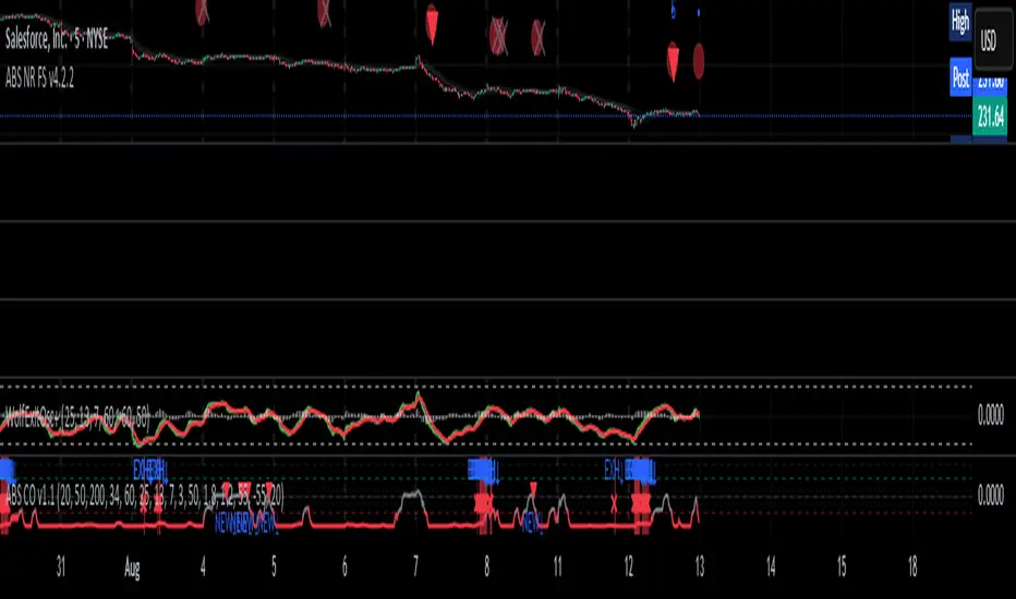
Hypothesis TF Strategy EvaluationThis script provides a statistical evaluation framework for trend-following strategies by examining whether mean returns (measured here as 1-period Rate of Change, ROC) differ significantly across different price quantile groups.
Specifically, it:
Calculates rolling 25th (Q1) and 75th (Q3) percentile levels of price over a user-defined window.
Classifies returns into three groups based on whether price is above Q3, between Q1 and Q3, or below Q1.
Computes mean returns and sample sizes for each group.
Performs Welch's t-tests (which account for unequal variances) between groups to assess if their mean returns differ significantly.
Displays results in two tables:
Summary Table: Shows mean ROC and number of observations for each group.
Hypothesis Testing Table: Shows pairwise t-statistics with significance stars for 95% and 99% confidence levels.
Key Features
Rolling quantile calculations: Captures local price distributions dynamically.
Robust hypothesis testing: Welch's t-test allows for heteroskedasticity between groups.
Significance indicators: Easy visual interpretation with "*" (95%) and "**" (99%) significance levels.
Visual aids: Plots Q1 and Q3 levels on the price chart for intuitive understanding.
Extensible and transparent: Fully commented code that emphasizes the evaluation process rather than trading signals.
Important Notes
Not a trading strategy: This script is intended as a tool for research and validation, not as a standalone trading system.
Look-ahead bias caution: The calculation carefully avoids look-ahead bias by computing quantiles and ROC values only on past data at each point.
Users must ensure look-ahead bias is removed when applying this or similar methods, as look-ahead bias would artificially inflate performance and statistical significance.
The statistical tests rely on the assumption of independent samples, which might not fully hold in financial time series but still provide useful insights
Usage Suggestions
Use this evaluation framework to validate hypotheses about the behavior of returns under different price regimes.
Integrate with your strategy development workflow to test whether certain market conditions produce statistically distinct return distributions.
Example
In this example, the script was run with a quantile length of 20 bars and a lookback of 500 bars for ROC classification.
We consider a simple hypothetical "strategy":
Go long if the previous bar closed above Q3 the 75th percentile).
Go short if the previous bar closed below Q1 (the 25th percentile).
Stay in cash if the previous close was between Q1 and Q3.
The screenshot below demonstrates the results of this evaluation. Surprisingly, the "long" group shows a negative average return, while the "short" group has a positive average return, indicating mean reversion rather than trend following.
The hypothesis testing table confirms that the only statistically significant difference (at 95% or higher confidence) is between the above Q3 and below Q1 groups, suggesting a meaningful divergence in their return behavior.
This highlights how this framework can help validate or challenge intuitive assumptions about strategy performance through rigorous statistical testing.
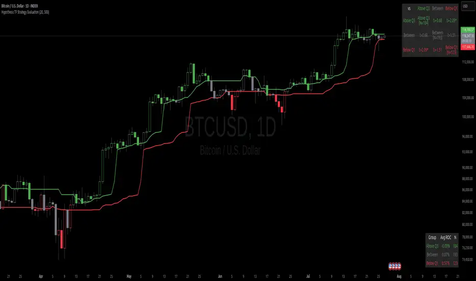
Supertrend with ADX & MTF MA Filter# **Supertrend with ADX & MTF MA Filter - Comprehensive Explanation**
---
## **1. Purpose of This Indicator**
This indicator combines three powerful technical analysis tools to create a robust trading system:
✅ **Supertrend** (Trend-following)
✅ **ADX Filter** (Trend strength confirmation)
✅ **MTF MA Filter** (Multi-timeframe trend direction confirmation)
**Primary Goals:**
✔ **Identify high-probability trend reversals** with confirmation from multiple indicators
✔ **Filter out weak trends** using ADX (Average Directional Index)
✔ **Add higher timeframe context** with MTF (Multi-TimeFrame) Moving Average
✔ **Reduce false signals** by requiring confluence between all three components
---
## **2. Core Logic & Components**
### **A. Supertrend (Base Indicator)**
- **Calculation:**
```pine
up = hl2 - (Multiplier * ATR(Periods))
dn = hl2 + (Multiplier * ATR(Periods))
```
- **Bullish trend** when price > `up` (green line)
- **Bearish trend** when price < `dn` (red line)
- **Why Supertrend?**
- Simple yet effective trend-following system
- Adapts to volatility via ATR (Average True Range)
---
### **B. ADX Filter (Trend Strength Confirmation)**
- **ADX Calculation:**
```pine
= calcADX(adxLength, adxSmoothing)
strongTrend = adxVal >= adxThreshold
```
- **ADX > Threshold (Default: 20)** = Strong trend
- **DI+ > DI-** = Bullish momentum
- **DI- > DI+** = Bearish momentum
- **Why ADX?**
- Avoids trading in choppy markets (low ADX = weak trend)
- Confirms if Supertrend signals occur in a strong trend
---
### **C. MTF MA Filter (Higher Timeframe Trend Alignment)**
- **Moving Average Calculation:**
```pine
= getMA(maSource, maLength, maType, maTF)
```
- **MA Type:** SMA, EMA, WMA, or DEMA
- **Timeframe:** Any (1m, 5m, 1H, 4H, D, W, M)
- **Trend Direction:**
- **Buy Signal:** MA must be **rising**
- **Sell Signal:** MA must be **falling**
- **Why MTF MA?**
- Aligns trades with the **higher timeframe trend**
- Reduces counter-trend entries
---
## **3. How to Use This Indicator**
### **A. Buy Conditions (All Must Be True)**
1. **Supertrend turns bullish** (price crosses above `up` line)
2. **ADX ≥ Threshold** (trend is strong)
3. **Higher timeframe MA is rising** (confirms bullish bias)
### **B. Sell Conditions (All Must Be True)**
1. **Supertrend turns bearish** (price crosses below `dn` line)
2. **ADX ≥ Threshold** (trend is strong)
3. **Higher timeframe MA is falling** (confirms bearish bias)
### **C. Recommended Settings**
| Parameter | Recommended Value | Description |
|-----------|------------------|-------------|
| **ATR Period** | 14 | Sensitivity of Supertrend |
| **Multiplier** | 1.5-3.0 | Adjust for volatility |
| **ADX Threshold** | 20-25 | Higher = stricter trend filter |
| **MA Length** | 20-50 | Smoothness of trend filter |
| **MA Timeframe** | 1H/D | Align with trading style |
---
## **4. Trading Strategies**
### **A. Trend-Following Strategy**
- **Enter:** When all 3 conditions align (Supertrend + ADX + MA)
- **Exit:** When Supertrend flips or ADX drops below threshold
### **B. Pullback Strategy**
- **Wait for:**
- Supertrend in trend direction
- ADX remains strong
- MA still aligned
- **Enter:** On pullback to Supertrend line
### **C. Multi-Timeframe Confirmation**
- **Intraday traders:** Use 4H/D MA for trend bias
- **Swing traders:** Use D/W MA for trend bias
---
## **5. Advantages Over Standard Supertrend**
✔ **Fewer false signals** (ADX filters weak trends)
✔ **Higher timeframe alignment** (avoids trading against larger trends)
✔ **Customizable MA types** (SMA, EMA, WMA, DEMA)
✔ **Works on all markets** (stocks, forex, crypto)
---
### **Final Thoughts**
This indicator is designed for traders who want **high-confidence trend signals** by combining:
🔹 **Supertrend** (entry trigger)
🔹 **ADX** (trend strength filter)
🔹 **MTF MA** (higher timeframe trend alignment)
By requiring all three components to align, it significantly improves signal quality compared to standalone Supertrend systems.
**→ Best for:** Swing trading, trend-following, and avoiding choppy markets.
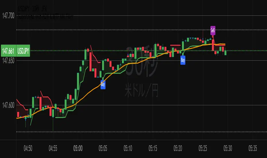
DA Cloud - DynamicDA Cloud - Dynamic | Detailed Overview
🌟 What Makes This Indicator Special
The DA Cloud - Dynamic is an advanced technical analysis tool that creates adaptive support and resistance zones that expand and contract based on market volatility. Unlike traditional static indicators, this cloud system "breathes" with the market, providing dynamic levels that adjust to changing market conditions.
📊 Core Components
1. Multi-Layered Cloud Structure
Resistance Cloud (Red): Three dynamic resistance levels (RL1, RL2, RL3) with intermediate channels (RC1, RC2)
Support Cloud (Green): Three dynamic support levels (SL1, SL2, SL3) with intermediate channels (SC1, SC2)
Trend Cloud (Blue): Five trend lines (TU2, TU1, TM, TL1, TL2) that flow through the center
Confirmation Line (Purple): A fast-reacting line that confirms trend changes
2. Forward Displacement Technology
The entire cloud system is projected 21 bars into the future (Fibonacci number), allowing traders to see potential support and resistance levels before price reaches them. This predictive element is inspired by Ichimoku Cloud theory but enhanced with modern volatility dynamics.
🔬 How It Works (Without Revealing the Secret Sauce)
Volatility-Responsive Design
The indicator continuously measures market volatility across multiple timeframes
During high volatility periods (like major breakouts), clouds expand dramatically
During consolidation, clouds contract and tighten around price
This creates a "breathing" effect that adapts to market conditions
Multi-Timeframe Analysis
Incorporates Fibonacci sequence periods (3, 13, 21, 34, 55) for calculations
Blends short-term responsiveness with long-term stability
Creates smooth, flowing lines that filter out market noise
Dynamic Level Calculation
Levels are not fixed percentages or static bands
Each level adapts based on current market structure and volatility
Channel lines (RC1, RC2, SC1, SC2) provide intermediate support/resistance
🎯 Key Features
1. Touch Point Detection
Colored dots appear when price touches key levels
Red dots = resistance touch
Green dots = support touch
Blue dots = trend median touch
2. Entry/Exit Signals
"Cloud Entry" labels when confirmation line crosses above SL1
"Cloud Exit" labels when confirmation line crosses below RL1
Background color changes based on bullish/bearish bias
3. Information Table
Real-time display of key levels (RL1, TM, SL1)
Current bias indicator (BULLISH/BEARISH)
Updates dynamically as market moves
⚙️ Customization Options
Main Controls:
Sensitivity (5-50): How responsive clouds are to price movements
Smoothing (1-50): Controls the flow and smoothness of cloud lines
Forward Displacement (0-50): How many bars to project the cloud forward
Advanced Volatility Settings:
Volatility Lookback (50-1000): Period for establishing volatility baseline
Volatility Smoothing (1-50): Reduces spikes in volatility expansion
Expansion Power (0.1-2.0): Controls how dramatically clouds expand
Range Divisor (1.0-20.0): Master control for overall cloud width
Level Spacing:
Individual multipliers for each resistance and support level
Allows fine-tuning of cloud structure to match different markets
Trend Spacing:
Separate controls for inner and outer trend bands
Customize the trend cloud density
📈 Trading Applications
1. Trend Identification
Price above TM (Trend Median) = Bullish bias
Price below TM = Bearish bias
Cloud color and width indicate trend strength
2. Support/Resistance Trading
Use RL1/SL1 as primary targets and reversal zones
RC1/RC2 and SC1/SC2 provide intermediate levels
RL3/SL3 mark extreme levels often seen at major tops/bottoms
3. Volatility Analysis
Expanding clouds signal increasing volatility and potential big moves
Contracting clouds indicate consolidation and potential breakout setup
Cloud width helps with position sizing and risk management
4. Multi-Timeframe Confirmation
Works on all timeframes from 1-minute to monthly
Higher timeframes show major market structure
Lower timeframes provide precise entry/exit points
🎓 Best Practices
Combine with Volume: High volume at cloud levels increases reliability
Watch for Touch Clusters: Multiple touches at a level indicate strength
Monitor Cloud Expansion: Sudden expansion often precedes major moves
Use Multiple Timeframes: Confirm signals across different time periods
Respect the Trend Median: This is often the most important level
⚡ Performance Notes
Optimized for up to 2000 bars of historical data
Smooth performance with 500+ lines and labels
Works on all markets: Crypto, Forex, Stocks, Commodities
📝 Version Info
Current Version: 1.0
Dynamic volatility expansion system
Full customization suite
Touch point detection
Entry/exit signals
Forward displacement projection
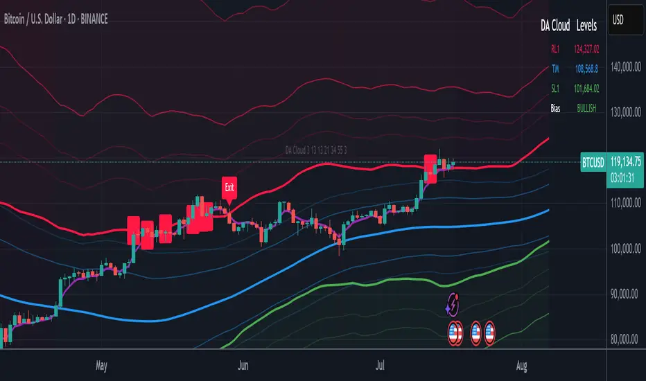
All SMAs Bullish/Bearish Screener (Enhanced)All SMAs Bullish/Bearish Screener Enhanced: Uncover High-Conviction Trend Alignments with Confidence
Description:
Are you ready to elevate your trading from mere guesswork to precise, data-driven decisions? The "All SMAs Bullish/Bearish Screener Enhanced" is not just another indicator; it's a sophisticated, yet user-friendly, trend-following powerhouse designed to cut through market noise and pinpoint high-probability trading opportunities. Built on the foundational strength of comprehensive Moving Average confluence and fortified with critical confirmation signals from Momentum, Volume, and Relative Strength, this script empowers you to identify truly robust trends and manage your trades with unparalleled clarity.
The Power of Multi-Factor Confluence: Beyond Simple Averages
In the unpredictable world of financial markets, true strength or weakness is rarely an isolated event. It's the harmonious alignment of multiple technical factors that signals a high-conviction move. While our original "All SMAs Bullish/Bearish Screener" intelligently identified stocks where price was consistently above or below a full spectrum of Simple Moving Averages (5, 10, 20, 50, 100, 200), this Enhanced version takes it a crucial step further.
We've integrated a powerful three-pronged confirmation system to filter out weaker signals and highlight only the most compelling setups:
Momentum (Rate of Change - ROC): A strong trend isn't just about price direction; it's about the speed and intensity of that movement. Positive momentum confirms that buyers are still aggressively pushing price higher (for bullish signals), while negative momentum validates selling pressure (for bearish signals).
Volume: No trend is truly trustworthy without the backing of smart money. Above-average volume accompanying an "All SMAs" alignment signifies strong institutional participation and conviction behind the move. It separates genuine trend starts from speculative whims.
Relative Strength Index (RSI): This versatile oscillator ensures the trend isn't just "there," but that it's developing healthily. We use RSI to confirm a bullish bias (above 50) or a bearish bias (below 50), adding another layer of confidence to the direction.
When the price aligns above ALL six critical SMAs, and is simultaneously confirmed by robust positive momentum, healthy volume, and a bullish RSI bias, you have an exceptionally strong "STRONGLY BULLISH" signal. This confluence often precedes sustained upward moves, signaling prime accumulation phases. Conversely, a "STRONGLY BEARISH" signal, where price is below ALL SMAs with negative momentum, confirming volume, and a bearish RSI bias, indicates powerful distribution and potential for significant downside.
How to Use This Enhanced Screener:
Add to Chart: Go to TradingView's Pine Editor, paste the script, and click "Add to Chart."
Customize Parameters: Fine-tune the lengths of your SMAs, RSI, Momentum, and Volume averages via the indicator's settings. Experiment to find what best suits your trading style and the assets you trade.
Choose Your Timeframe Wisely:
Daily (1D) and 4-Hour (240 min) are highly recommended. These timeframes cut through intraday noise and provide more reliable, actionable signals for swing and position trading.
Shorter timeframes (e.g., 15min, 60min) can be used by advanced day traders for very short-term entries, but be aware of increased volatility and noise.
Visual Confirmation:
Green/Red Triangles: Appear on your chart, indicating confirmed bullish or bearish signals.
Background Color: The chart background will subtly turn lime green for "STRONGLY BULLISH" and red for "STRONGLY BEARISH" conditions.
On-Chart Status Table: A clear table displays the current signal status ("STRONGLY BULLISH/BEARISH," or "SMAs Mixed") for immediate feedback.
Set Up Alerts (Your Primary Screener Tool): This is the game-changer! Create custom alerts on TradingView based on the "Confirmed Bullish Trade" and "Confirmed Bearish Trade" conditions. Receive instant notifications (email, pop-up, mobile) for any stock in your watchlist that meets these stringent criteria. This allows you to scan the entire market effortlessly and act decisively.
Strategic Stop-Loss Placement: The Trader's Lifeline
Even the most robust signals can fail. Protecting your capital is paramount. For this trend-following strategy, your stop-loss should be placed where the underlying trend structure is broken.
For a "STRONGLY BULLISH" Trade: Place your stop-loss just below the most recent significant swing low (higher low). This is the last point where buyers stepped in to support the price. If price breaks below this, your bullish thesis is invalidated.
For a "STRONGLY BEARISH" Trade: Place your stop-loss just above the most recent significant swing high (lower high). If price breaks above this, your bearish thesis is invalidated.
Alternatively, consider placing your stop-loss just below the 20-period SMA (for bullish trades) or above the 20-period SMA (for bearish trades). A significant close beyond this intermediate-term average often indicates a critical shift in momentum. Always ensure your chosen stop-loss adheres to your pre-defined risk per trade (e.g., 1-2% of capital).
Disciplined Profit Booking: Maximizing Gains
Just as important as knowing when you're wrong is knowing when to take profits.
Trailing Stop-Loss: As your trade moves into profit, trail your stop-loss upwards (for longs) or downwards (for shorts). You can trail it using:
Previous Swing Lows/Highs: Move your stop to just below each new higher low (for longs) or just above each new lower high (for shorts).
A Moving Average (e.g., 10-period or 20-period SMA): If price closes below your chosen trailing SMA, exit. This allows you to ride the trend while protecting accumulated profits.
Target Levels: Identify potential resistance levels (for longs) or support levels (for shorts) using pivot points, previous highs/lows, or Fibonacci extensions. Consider taking partial profits at these levels and letting the rest run with a trailing stop.
Loss of Confluence: If the "STRONGLY BULLISH/BEARISH" condition ceases to be met (e.g., RSI crosses below 50, or volume drops significantly), this can be a signal to reduce or exit your position, even if your stop-loss hasn't been hit.
The "All SMAs Bullish/Bearish Screener Enhanced" is your comprehensive partner in navigating the markets. By combining robust trend identification with critical confirmation signals and disciplined risk management, you're equipped to make smarter, more confident trading decisions. Add it to your favorites and unlock a new level of precision in your trading journey!
#PineScript #TradingView #SMA #MovingAverage #TrendFollowing #StockScreener #TechnicalAnalysis #Bullish #Bearish #QQQ #Momentum #Volume #RSI #SPY #TradingStrategy #Enhanced #Signals #Analysis #DayTrading #SwingTrading
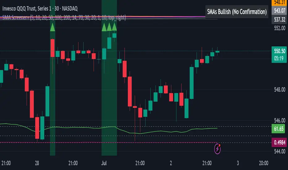
Tensor Market Analysis Engine (TMAE)# Tensor Market Analysis Engine (TMAE)
## Advanced Multi-Dimensional Mathematical Analysis System
*Where Quantum Mathematics Meets Market Structure*
---
## 🎓 THEORETICAL FOUNDATION
The Tensor Market Analysis Engine represents a revolutionary synthesis of three cutting-edge mathematical frameworks that have never before been combined for comprehensive market analysis. This indicator transcends traditional technical analysis by implementing advanced mathematical concepts from quantum mechanics, information theory, and fractal geometry.
### 🌊 Multi-Dimensional Volatility with Jump Detection
**Hawkes Process Implementation:**
The TMAE employs a sophisticated Hawkes process approximation for detecting self-exciting market jumps. Unlike traditional volatility measures that treat price movements as independent events, the Hawkes process recognizes that market shocks cluster and exhibit memory effects.
**Mathematical Foundation:**
```
Intensity λ(t) = μ + Σ α(t - Tᵢ)
```
Where market jumps at times Tᵢ increase the probability of future jumps through the decay function α, controlled by the Hawkes Decay parameter (0.5-0.99).
**Mahalanobis Distance Calculation:**
The engine calculates volatility jumps using multi-dimensional Mahalanobis distance across up to 5 volatility dimensions:
- **Dimension 1:** Price volatility (standard deviation of returns)
- **Dimension 2:** Volume volatility (normalized volume fluctuations)
- **Dimension 3:** Range volatility (high-low spread variations)
- **Dimension 4:** Correlation volatility (price-volume relationship changes)
- **Dimension 5:** Microstructure volatility (intrabar positioning analysis)
This creates a volatility state vector that captures market behavior impossible to detect with traditional single-dimensional approaches.
### 📐 Hurst Exponent Regime Detection
**Fractal Market Hypothesis Integration:**
The TMAE implements advanced Rescaled Range (R/S) analysis to calculate the Hurst exponent in real-time, providing dynamic regime classification:
- **H > 0.6:** Trending (persistent) markets - momentum strategies optimal
- **H < 0.4:** Mean-reverting (anti-persistent) markets - contrarian strategies optimal
- **H ≈ 0.5:** Random walk markets - breakout strategies preferred
**Adaptive R/S Analysis:**
Unlike static implementations, the TMAE uses adaptive windowing that adjusts to market conditions:
```
H = log(R/S) / log(n)
```
Where R is the range of cumulative deviations and S is the standard deviation over period n.
**Dynamic Regime Classification:**
The system employs hysteresis to prevent regime flipping, requiring sustained Hurst values before regime changes are confirmed. This prevents false signals during transitional periods.
### 🔄 Transfer Entropy Analysis
**Information Flow Quantification:**
Transfer entropy measures the directional flow of information between price and volume, revealing lead-lag relationships that indicate future price movements:
```
TE(X→Y) = Σ p(yₜ₊₁, yₜ, xₜ) log
```
**Causality Detection:**
- **Volume → Price:** Indicates accumulation/distribution phases
- **Price → Volume:** Suggests retail participation or momentum chasing
- **Balanced Flow:** Market equilibrium or transition periods
The system analyzes multiple lag periods (2-20 bars) to capture both immediate and structural information flows.
---
## 🔧 COMPREHENSIVE INPUT SYSTEM
### Core Parameters Group
**Primary Analysis Window (10-100, Default: 50)**
The fundamental lookback period affecting all calculations. Optimization by timeframe:
- **1-5 minute charts:** 20-30 (rapid adaptation to micro-movements)
- **15 minute-1 hour:** 30-50 (balanced responsiveness and stability)
- **4 hour-daily:** 50-100 (smooth signals, reduced noise)
- **Asset-specific:** Cryptocurrency 20-35, Stocks 35-50, Forex 40-60
**Signal Sensitivity (0.1-2.0, Default: 0.7)**
Master control affecting all threshold calculations:
- **Conservative (0.3-0.6):** High-quality signals only, fewer false positives
- **Balanced (0.7-1.0):** Optimal risk-reward ratio for most trading styles
- **Aggressive (1.1-2.0):** Maximum signal frequency, requires careful filtering
**Signal Generation Mode:**
- **Aggressive:** Any component signals (highest frequency)
- **Confluence:** 2+ components agree (balanced approach)
- **Conservative:** All 3 components align (highest quality)
### Volatility Jump Detection Group
**Volatility Dimensions (2-5, Default: 3)**
Determines the mathematical space complexity:
- **2D:** Price + Volume volatility (suitable for clean markets)
- **3D:** + Range volatility (optimal for most conditions)
- **4D:** + Correlation volatility (advanced multi-asset analysis)
- **5D:** + Microstructure volatility (maximum sensitivity)
**Jump Detection Threshold (1.5-4.0σ, Default: 3.0σ)**
Standard deviations required for volatility jump classification:
- **Cryptocurrency:** 2.0-2.5σ (naturally volatile)
- **Stock Indices:** 2.5-3.0σ (moderate volatility)
- **Forex Major Pairs:** 3.0-3.5σ (typically stable)
- **Commodities:** 2.0-3.0σ (varies by commodity)
**Jump Clustering Decay (0.5-0.99, Default: 0.85)**
Hawkes process memory parameter:
- **0.5-0.7:** Fast decay (jumps treated as independent)
- **0.8-0.9:** Moderate clustering (realistic market behavior)
- **0.95-0.99:** Strong clustering (crisis/event-driven markets)
### Hurst Exponent Analysis Group
**Calculation Method Options:**
- **Classic R/S:** Original Rescaled Range (fast, simple)
- **Adaptive R/S:** Dynamic windowing (recommended for trading)
- **DFA:** Detrended Fluctuation Analysis (best for noisy data)
**Trending Threshold (0.55-0.8, Default: 0.60)**
Hurst value defining persistent market behavior:
- **0.55-0.60:** Weak trend persistence
- **0.65-0.70:** Clear trending behavior
- **0.75-0.80:** Strong momentum regimes
**Mean Reversion Threshold (0.2-0.45, Default: 0.40)**
Hurst value defining anti-persistent behavior:
- **0.35-0.45:** Weak mean reversion
- **0.25-0.35:** Clear ranging behavior
- **0.15-0.25:** Strong reversion tendency
### Transfer Entropy Parameters Group
**Information Flow Analysis:**
- **Price-Volume:** Classic flow analysis for accumulation/distribution
- **Price-Volatility:** Risk flow analysis for sentiment shifts
- **Multi-Timeframe:** Cross-timeframe causality detection
**Maximum Lag (2-20, Default: 5)**
Causality detection window:
- **2-5 bars:** Immediate causality (scalping)
- **5-10 bars:** Short-term flow (day trading)
- **10-20 bars:** Structural flow (swing trading)
**Significance Threshold (0.05-0.3, Default: 0.15)**
Minimum entropy for signal generation:
- **0.05-0.10:** Detect subtle information flows
- **0.10-0.20:** Clear causality only
- **0.20-0.30:** Very strong flows only
---
## 🎨 ADVANCED VISUAL SYSTEM
### Tensor Volatility Field Visualization
**Five-Layer Resonance Bands:**
The tensor field creates dynamic support/resistance zones that expand and contract based on mathematical field strength:
- **Core Layer (Purple):** Primary tensor field with highest intensity
- **Layer 2 (Neutral):** Secondary mathematical resonance
- **Layer 3 (Info Blue):** Tertiary harmonic frequencies
- **Layer 4 (Warning Gold):** Outer field boundaries
- **Layer 5 (Success Green):** Maximum field extension
**Field Strength Calculation:**
```
Field Strength = min(3.0, Mahalanobis Distance × Tensor Intensity)
```
The field amplitude adjusts to ATR and mathematical distance, creating dynamic zones that respond to market volatility.
**Radiation Line Network:**
During active tensor states, the system projects directional radiation lines showing field energy distribution:
- **8 Directional Rays:** Complete angular coverage
- **Tapering Segments:** Progressive transparency for natural visual flow
- **Pulse Effects:** Enhanced visualization during volatility jumps
### Dimensional Portal System
**Portal Mathematics:**
Dimensional portals visualize regime transitions using category theory principles:
- **Green Portals (◉):** Trending regime detection (appear below price for support)
- **Red Portals (◎):** Mean-reverting regime (appear above price for resistance)
- **Yellow Portals (○):** Random walk regime (neutral positioning)
**Tensor Trail Effects:**
Each portal generates 8 trailing particles showing mathematical momentum:
- **Large Particles (●):** Strong mathematical signal
- **Medium Particles (◦):** Moderate signal strength
- **Small Particles (·):** Weak signal continuation
- **Micro Particles (˙):** Signal dissipation
### Information Flow Streams
**Particle Stream Visualization:**
Transfer entropy creates flowing particle streams indicating information direction:
- **Upward Streams:** Volume leading price (accumulation phases)
- **Downward Streams:** Price leading volume (distribution phases)
- **Stream Density:** Proportional to information flow strength
**15-Particle Evolution:**
Each stream contains 15 particles with progressive sizing and transparency, creating natural flow visualization that makes information transfer immediately apparent.
### Fractal Matrix Grid System
**Multi-Timeframe Fractal Levels:**
The system calculates and displays fractal highs/lows across five Fibonacci periods:
- **8-Period:** Short-term fractal structure
- **13-Period:** Intermediate-term patterns
- **21-Period:** Primary swing levels
- **34-Period:** Major structural levels
- **55-Period:** Long-term fractal boundaries
**Triple-Layer Visualization:**
Each fractal level uses three-layer rendering:
- **Shadow Layer:** Widest, darkest foundation (width 5)
- **Glow Layer:** Medium white core line (width 3)
- **Tensor Layer:** Dotted mathematical overlay (width 1)
**Intelligent Labeling System:**
Smart spacing prevents label overlap using ATR-based minimum distances. Labels include:
- **Fractal Period:** Time-based identification
- **Topological Class:** Mathematical complexity rating (0, I, II, III)
- **Price Level:** Exact fractal price
- **Mahalanobis Distance:** Current mathematical field strength
- **Hurst Exponent:** Current regime classification
- **Anomaly Indicators:** Visual strength representations (○ ◐ ● ⚡)
### Wick Pressure Analysis
**Rejection Level Mathematics:**
The system analyzes candle wick patterns to project future pressure zones:
- **Upper Wick Analysis:** Identifies selling pressure and resistance zones
- **Lower Wick Analysis:** Identifies buying pressure and support zones
- **Pressure Projection:** Extends lines forward based on mathematical probability
**Multi-Layer Glow Effects:**
Wick pressure lines use progressive transparency (1-8 layers) creating natural glow effects that make pressure zones immediately visible without cluttering the chart.
### Enhanced Regime Background
**Dynamic Intensity Mapping:**
Background colors reflect mathematical regime strength:
- **Deep Transparency (98% alpha):** Subtle regime indication
- **Pulse Intensity:** Based on regime strength calculation
- **Color Coding:** Green (trending), Red (mean-reverting), Neutral (random)
**Smoothing Integration:**
Regime changes incorporate 10-bar smoothing to prevent background flicker while maintaining responsiveness to genuine regime shifts.
### Color Scheme System
**Six Professional Themes:**
- **Dark (Default):** Professional trading environment optimization
- **Light:** High ambient light conditions
- **Classic:** Traditional technical analysis appearance
- **Neon:** High-contrast visibility for active trading
- **Neutral:** Minimal distraction focus
- **Bright:** Maximum visibility for complex setups
Each theme maintains mathematical accuracy while optimizing visual clarity for different trading environments and personal preferences.
---
## 📊 INSTITUTIONAL-GRADE DASHBOARD
### Tensor Field Status Section
**Field Strength Display:**
Real-time Mahalanobis distance calculation with dynamic emoji indicators:
- **⚡ (Lightning):** Extreme field strength (>1.5× threshold)
- **● (Solid Circle):** Strong field activity (>1.0× threshold)
- **○ (Open Circle):** Normal field state
**Signal Quality Rating:**
Democratic algorithm assessment:
- **ELITE:** All 3 components aligned (highest probability)
- **STRONG:** 2 components aligned (good probability)
- **GOOD:** 1 component active (moderate probability)
- **WEAK:** No clear component signals
**Threshold and Anomaly Monitoring:**
- **Threshold Display:** Current mathematical threshold setting
- **Anomaly Level (0-100%):** Combined volatility and volume spike measurement
- **>70%:** High anomaly (red warning)
- **30-70%:** Moderate anomaly (orange caution)
- **<30%:** Normal conditions (green confirmation)
### Tensor State Analysis Section
**Mathematical State Classification:**
- **↑ BULL (Tensor State +1):** Trending regime with bullish bias
- **↓ BEAR (Tensor State -1):** Mean-reverting regime with bearish bias
- **◈ SUPER (Tensor State 0):** Random walk regime (neutral)
**Visual State Gauge:**
Five-circle progression showing tensor field polarity:
- **🟢🟢🟢⚪⚪:** Strong bullish mathematical alignment
- **⚪⚪🟡⚪⚪:** Neutral/transitional state
- **⚪⚪🔴🔴🔴:** Strong bearish mathematical alignment
**Trend Direction and Phase Analysis:**
- **📈 BULL / 📉 BEAR / ➡️ NEUTRAL:** Primary trend classification
- **🌪️ CHAOS:** Extreme information flow (>2.0 flow strength)
- **⚡ ACTIVE:** Strong information flow (1.0-2.0 flow strength)
- **😴 CALM:** Low information flow (<1.0 flow strength)
### Trading Signals Section
**Real-Time Signal Status:**
- **🟢 ACTIVE / ⚪ INACTIVE:** Long signal availability
- **🔴 ACTIVE / ⚪ INACTIVE:** Short signal availability
- **Components (X/3):** Active algorithmic components
- **Mode Display:** Current signal generation mode
**Signal Strength Visualization:**
Color-coded component count:
- **Green:** 3/3 components (maximum confidence)
- **Aqua:** 2/3 components (good confidence)
- **Orange:** 1/3 components (moderate confidence)
- **Gray:** 0/3 components (no signals)
### Performance Metrics Section
**Win Rate Monitoring:**
Estimated win rates based on signal quality with emoji indicators:
- **🔥 (Fire):** ≥60% estimated win rate
- **👍 (Thumbs Up):** 45-59% estimated win rate
- **⚠️ (Warning):** <45% estimated win rate
**Mathematical Metrics:**
- **Hurst Exponent:** Real-time fractal dimension (0.000-1.000)
- **Information Flow:** Volume/price leading indicators
- **📊 VOL:** Volume leading price (accumulation/distribution)
- **💰 PRICE:** Price leading volume (momentum/speculation)
- **➖ NONE:** Balanced information flow
- **Volatility Classification:**
- **🔥 HIGH:** Above 1.5× jump threshold
- **📊 NORM:** Normal volatility range
- **😴 LOW:** Below 0.5× jump threshold
### Market Structure Section (Large Dashboard)
**Regime Classification:**
- **📈 TREND:** Hurst >0.6, momentum strategies optimal
- **🔄 REVERT:** Hurst <0.4, contrarian strategies optimal
- **🎲 RANDOM:** Hurst ≈0.5, breakout strategies preferred
**Mathematical Field Analysis:**
- **Dimensions:** Current volatility space complexity (2D-5D)
- **Hawkes λ (Lambda):** Self-exciting jump intensity (0.00-1.00)
- **Jump Status:** 🚨 JUMP (active) / ✅ NORM (normal)
### Settings Summary Section (Large Dashboard)
**Active Configuration Display:**
- **Sensitivity:** Current master sensitivity setting
- **Lookback:** Primary analysis window
- **Theme:** Active color scheme
- **Method:** Hurst calculation method (Classic R/S, Adaptive R/S, DFA)
**Dashboard Sizing Options:**
- **Small:** Essential metrics only (mobile/small screens)
- **Normal:** Balanced information density (standard desktop)
- **Large:** Maximum detail (multi-monitor setups)
**Position Options:**
- **Top Right:** Standard placement (avoids price action)
- **Top Left:** Wide chart optimization
- **Bottom Right:** Recent price focus (scalping)
- **Bottom Left:** Maximum price visibility (swing trading)
---
## 🎯 SIGNAL GENERATION LOGIC
### Multi-Component Convergence System
**Component Signal Architecture:**
The TMAE generates signals through sophisticated component analysis rather than simple threshold crossing:
**Volatility Component:**
- **Jump Detection:** Mahalanobis distance threshold breach
- **Hawkes Intensity:** Self-exciting process activation (>0.2)
- **Multi-dimensional:** Considers all volatility dimensions simultaneously
**Hurst Regime Component:**
- **Trending Markets:** Price above SMA-20 with positive momentum
- **Mean-Reverting Markets:** Price at Bollinger Band extremes
- **Random Markets:** Bollinger squeeze breakouts with directional confirmation
**Transfer Entropy Component:**
- **Volume Leadership:** Information flow from volume to price
- **Volume Spike:** Volume 110%+ above 20-period average
- **Flow Significance:** Above entropy threshold with directional bias
### Democratic Signal Weighting
**Signal Mode Implementation:**
- **Aggressive Mode:** Any single component triggers signal
- **Confluence Mode:** Minimum 2 components must agree
- **Conservative Mode:** All 3 components must align
**Momentum Confirmation:**
All signals require momentum confirmation:
- **Long Signals:** RSI >50 AND price >EMA-9
- **Short Signals:** RSI <50 AND price 0.6):**
- **Increase Sensitivity:** Catch momentum continuation
- **Lower Mean Reversion Threshold:** Avoid counter-trend signals
- **Emphasize Volume Leadership:** Institutional accumulation/distribution
- **Tensor Field Focus:** Use expansion for trend continuation
- **Signal Mode:** Aggressive or Confluence for trend following
**Range-Bound Markets (Hurst <0.4):**
- **Decrease Sensitivity:** Avoid false breakouts
- **Lower Trending Threshold:** Quick regime recognition
- **Focus on Price Leadership:** Retail sentiment extremes
- **Fractal Grid Emphasis:** Support/resistance trading
- **Signal Mode:** Conservative for high-probability reversals
**Volatile Markets (High Jump Frequency):**
- **Increase Hawkes Decay:** Recognize event clustering
- **Higher Jump Threshold:** Avoid noise signals
- **Maximum Dimensions:** Capture full volatility complexity
- **Reduce Position Sizing:** Risk management adaptation
- **Enhanced Visuals:** Maximum information for rapid decisions
**Low Volatility Markets (Low Jump Frequency):**
- **Decrease Jump Threshold:** Capture subtle movements
- **Lower Hawkes Decay:** Treat moves as independent
- **Reduce Dimensions:** Simplify analysis
- **Increase Position Sizing:** Capitalize on compressed volatility
- **Minimal Visuals:** Reduce distraction in quiet markets
---
## 🚀 ADVANCED TRADING STRATEGIES
### The Mathematical Convergence Method
**Entry Protocol:**
1. **Fractal Grid Approach:** Monitor price approaching significant fractal levels
2. **Tensor Field Confirmation:** Verify field expansion supporting direction
3. **Portal Signal:** Wait for dimensional portal appearance
4. **ELITE/STRONG Quality:** Only trade highest quality mathematical signals
5. **Component Consensus:** Confirm 2+ components agree in Confluence mode
**Example Implementation:**
- Price approaching 21-period fractal high
- Tensor field expanding upward (bullish mathematical alignment)
- Green portal appears below price (trending regime confirmation)
- ELITE quality signal with 3/3 components active
- Enter long position with stop below fractal level
**Risk Management:**
- **Stop Placement:** Below/above fractal level that generated signal
- **Position Sizing:** Based on Mahalanobis distance (higher distance = smaller size)
- **Profit Targets:** Next fractal level or tensor field resistance
### The Regime Transition Strategy
**Regime Change Detection:**
1. **Monitor Hurst Exponent:** Watch for persistent moves above/below thresholds
2. **Portal Color Change:** Regime transitions show different portal colors
3. **Background Intensity:** Increasing regime background intensity
4. **Mathematical Confirmation:** Wait for regime confirmation (hysteresis)
**Trading Implementation:**
- **Trending Transitions:** Trade momentum breakouts, follow trend
- **Mean Reversion Transitions:** Trade range boundaries, fade extremes
- **Random Transitions:** Trade breakouts with tight stops
**Advanced Techniques:**
- **Multi-Timeframe:** Confirm regime on higher timeframe
- **Early Entry:** Enter on regime transition rather than confirmation
- **Regime Strength:** Larger positions during strong regime signals
### The Information Flow Momentum Strategy
**Flow Detection Protocol:**
1. **Monitor Transfer Entropy:** Watch for significant information flow shifts
2. **Volume Leadership:** Strong edge when volume leads price
3. **Flow Acceleration:** Increasing flow strength indicates momentum
4. **Directional Confirmation:** Ensure flow aligns with intended trade direction
**Entry Signals:**
- **Volume → Price Flow:** Enter during accumulation/distribution phases
- **Price → Volume Flow:** Enter on momentum confirmation breaks
- **Flow Reversal:** Counter-trend entries when flow reverses
**Optimization:**
- **Scalping:** Use immediate flow detection (2-5 bar lag)
- **Swing Trading:** Use structural flow (10-20 bar lag)
- **Multi-Asset:** Compare flow between correlated assets
### The Tensor Field Expansion Strategy
**Field Mathematics:**
The tensor field expansion indicates mathematical pressure building in market structure:
**Expansion Phases:**
1. **Compression:** Field contracts, volatility decreases
2. **Tension Building:** Mathematical pressure accumulates
3. **Expansion:** Field expands rapidly with directional movement
4. **Resolution:** Field stabilizes at new equilibrium
**Trading Applications:**
- **Compression Trading:** Prepare for breakout during field contraction
- **Expansion Following:** Trade direction of field expansion
- **Reversion Trading:** Fade extreme field expansion
- **Multi-Dimensional:** Consider all field layers for confirmation
### The Hawkes Process Event Strategy
**Self-Exciting Jump Trading:**
Understanding that market shocks cluster and create follow-on opportunities:
**Jump Sequence Analysis:**
1. **Initial Jump:** First volatility jump detected
2. **Clustering Phase:** Hawkes intensity remains elevated
3. **Follow-On Opportunities:** Additional jumps more likely
4. **Decay Period:** Intensity gradually decreases
**Implementation:**
- **Jump Confirmation:** Wait for mathematical jump confirmation
- **Direction Assessment:** Use other components for direction
- **Clustering Trades:** Trade subsequent moves during high intensity
- **Decay Exit:** Exit positions as Hawkes intensity decays
### The Fractal Confluence System
**Multi-Timeframe Fractal Analysis:**
Combining fractal levels across different periods for high-probability zones:
**Confluence Zones:**
- **Double Confluence:** 2 fractal levels align
- **Triple Confluence:** 3+ fractal levels cluster
- **Mathematical Confirmation:** Tensor field supports the level
- **Information Flow:** Transfer entropy confirms direction
**Trading Protocol:**
1. **Identify Confluence:** Find 2+ fractal levels within 1 ATR
2. **Mathematical Support:** Verify tensor field alignment
3. **Signal Quality:** Wait for STRONG or ELITE signal
4. **Risk Definition:** Use fractal level for stop placement
5. **Profit Targeting:** Next major fractal confluence zone
---
## ⚠️ COMPREHENSIVE RISK MANAGEMENT
### Mathematical Position Sizing
**Mahalanobis Distance Integration:**
Position size should inversely correlate with mathematical field strength:
```
Position Size = Base Size × (Threshold / Mahalanobis Distance)
```
**Risk Scaling Matrix:**
- **Low Field Strength (<2.0):** Standard position sizing
- **Moderate Field Strength (2.0-3.0):** 75% position sizing
- **High Field Strength (3.0-4.0):** 50% position sizing
- **Extreme Field Strength (>4.0):** 25% position sizing or no trade
### Signal Quality Risk Adjustment
**Quality-Based Position Sizing:**
- **ELITE Signals:** 100% of planned position size
- **STRONG Signals:** 75% of planned position size
- **GOOD Signals:** 50% of planned position size
- **WEAK Signals:** No position or paper trading only
**Component Agreement Scaling:**
- **3/3 Components:** Full position size
- **2/3 Components:** 75% position size
- **1/3 Components:** 50% position size or skip trade
### Regime-Adaptive Risk Management
**Trending Market Risk:**
- **Wider Stops:** Allow for trend continuation
- **Trend Following:** Trade with regime direction
- **Higher Position Size:** Trend probability advantage
- **Momentum Stops:** Trail stops based on momentum indicators
**Mean-Reverting Market Risk:**
- **Tighter Stops:** Quick exits on trend continuation
- **Contrarian Positioning:** Trade against extremes
- **Smaller Position Size:** Higher reversal failure rate
- **Level-Based Stops:** Use fractal levels for stops
**Random Market Risk:**
- **Breakout Focus:** Trade only clear breakouts
- **Tight Initial Stops:** Quick exit if breakout fails
- **Reduced Frequency:** Skip marginal setups
- **Range-Based Targets:** Profit targets at range boundaries
### Volatility-Adaptive Risk Controls
**High Volatility Periods:**
- **Reduced Position Size:** Account for wider price swings
- **Wider Stops:** Avoid noise-based exits
- **Lower Frequency:** Skip marginal setups
- **Faster Exits:** Take profits more quickly
**Low Volatility Periods:**
- **Standard Position Size:** Normal risk parameters
- **Tighter Stops:** Take advantage of compressed ranges
- **Higher Frequency:** Trade more setups
- **Extended Targets:** Allow for compressed volatility expansion
### Multi-Timeframe Risk Alignment
**Higher Timeframe Trend:**
- **With Trend:** Standard or increased position size
- **Against Trend:** Reduced position size or skip
- **Neutral Trend:** Standard position size with tight management
**Risk Hierarchy:**
1. **Primary:** Current timeframe signal quality
2. **Secondary:** Higher timeframe trend alignment
3. **Tertiary:** Mathematical field strength
4. **Quaternary:** Market regime classification
---
## 📚 EDUCATIONAL VALUE AND MATHEMATICAL CONCEPTS
### Advanced Mathematical Concepts
**Tensor Analysis in Markets:**
The TMAE introduces traders to tensor analysis, a branch of mathematics typically reserved for physics and advanced engineering. Tensors provide a framework for understanding multi-dimensional market relationships that scalar and vector analysis cannot capture.
**Information Theory Applications:**
Transfer entropy implementation teaches traders about information flow in markets, a concept from information theory that quantifies directional causality between variables. This provides intuition about market microstructure and participant behavior.
**Fractal Geometry in Trading:**
The Hurst exponent calculation exposes traders to fractal geometry concepts, helping understand that markets exhibit self-similar patterns across multiple timeframes. This mathematical insight transforms how traders view market structure.
**Stochastic Process Theory:**
The Hawkes process implementation introduces concepts from stochastic process theory, specifically self-exciting point processes. This provides mathematical framework for understanding why market events cluster and exhibit memory effects.
### Learning Progressive Complexity
**Beginner Mathematical Concepts:**
- **Volatility Dimensions:** Understanding multi-dimensional analysis
- **Regime Classification:** Learning market personality types
- **Signal Democracy:** Algorithmic consensus building
- **Visual Mathematics:** Interpreting mathematical concepts visually
**Intermediate Mathematical Applications:**
- **Mahalanobis Distance:** Statistical distance in multi-dimensional space
- **Rescaled Range Analysis:** Fractal dimension measurement
- **Information Entropy:** Quantifying uncertainty and causality
- **Field Theory:** Understanding mathematical fields in market context
**Advanced Mathematical Integration:**
- **Tensor Field Dynamics:** Multi-dimensional market force analysis
- **Stochastic Self-Excitation:** Event clustering and memory effects
- **Categorical Composition:** Mathematical signal combination theory
- **Topological Market Analysis:** Understanding market shape and connectivity
### Practical Mathematical Intuition
**Developing Market Mathematics Intuition:**
The TMAE serves as a bridge between abstract mathematical concepts and practical trading applications. Traders develop intuitive understanding of:
- **How markets exhibit mathematical structure beneath apparent randomness**
- **Why multi-dimensional analysis reveals patterns invisible to single-variable approaches**
- **How information flows through markets in measurable, predictable ways**
- **Why mathematical models provide probabilistic edges rather than certainties**
---
## 🔬 IMPLEMENTATION AND OPTIMIZATION
### Getting Started Protocol
**Phase 1: Observation (Week 1)**
1. **Apply with defaults:** Use standard settings on your primary trading timeframe
2. **Study visual elements:** Learn to interpret tensor fields, portals, and streams
3. **Monitor dashboard:** Observe how metrics change with market conditions
4. **No trading:** Focus entirely on pattern recognition and understanding
**Phase 2: Pattern Recognition (Week 2-3)**
1. **Identify signal patterns:** Note what market conditions produce different signal qualities
2. **Regime correlation:** Observe how Hurst regimes affect signal performance
3. **Visual confirmation:** Learn to read tensor field expansion and portal signals
4. **Component analysis:** Understand which components drive signals in different markets
**Phase 3: Parameter Optimization (Week 4-5)**
1. **Asset-specific tuning:** Adjust parameters for your specific trading instrument
2. **Timeframe optimization:** Fine-tune for your preferred trading timeframe
3. **Sensitivity adjustment:** Balance signal frequency with quality
4. **Visual customization:** Optimize colors and intensity for your trading environment
**Phase 4: Live Implementation (Week 6+)**
1. **Paper trading:** Test signals with hypothetical trades
2. **Small position sizing:** Begin with minimal risk during learning phase
3. **Performance tracking:** Monitor actual vs. expected signal performance
4. **Continuous optimization:** Refine settings based on real performance data
### Performance Monitoring System
**Signal Quality Tracking:**
- **ELITE Signal Win Rate:** Track highest quality signals separately
- **Component Performance:** Monitor which components provide best signals
- **Regime Performance:** Analyze performance across different market regimes
- **Timeframe Analysis:** Compare performance across different session times
**Mathematical Metric Correlation:**
- **Field Strength vs. Performance:** Higher field strength should correlate with better performance
- **Component Agreement vs. Win Rate:** More component agreement should improve win rates
- **Regime Alignment vs. Success:** Trading with mathematical regime should outperform
### Continuous Optimization Process
**Monthly Review Protocol:**
1. **Performance Analysis:** Review win rates, profit factors, and maximum drawdown
2. **Parameter Assessment:** Evaluate if current settings remain optimal
3. **Market Adaptation:** Adjust for changes in market character or volatility
4. **Component Weighting:** Consider if certain components should receive more/less emphasis
**Quarterly Deep Analysis:**
1. **Mathematical Model Validation:** Verify that mathematical relationships remain valid
2. **Regime Distribution:** Analyze time spent in different market regimes
3. **Signal Evolution:** Track how signal characteristics change over time
4. **Correlation Analysis:** Monitor correlations between different mathematical components
---
## 🌟 UNIQUE INNOVATIONS AND CONTRIBUTIONS
### Revolutionary Mathematical Integration
**First-Ever Implementations:**
1. **Multi-Dimensional Volatility Tensor:** First indicator to implement true tensor analysis for market volatility
2. **Real-Time Hawkes Process:** First trading implementation of self-exciting point processes
3. **Transfer Entropy Trading Signals:** First practical application of information theory for trade generation
4. **Democratic Component Voting:** First algorithmic consensus system for signal generation
5. **Fractal-Projected Signal Quality:** First system to predict signal quality at future price levels
### Advanced Visualization Innovations
**Mathematical Visualization Breakthroughs:**
- **Tensor Field Radiation:** Visual representation of mathematical field energy
- **Dimensional Portal System:** Category theory visualization for regime transitions
- **Information Flow Streams:** Real-time visual display of market information transfer
- **Multi-Layer Fractal Grid:** Intelligent spacing and projection system
- **Regime Intensity Mapping:** Dynamic background showing mathematical regime strength
### Practical Trading Innovations
**Trading System Advances:**
- **Quality-Weighted Signal Generation:** Signals rated by mathematical confidence
- **Regime-Adaptive Strategy Selection:** Automatic strategy optimization based on market personality
- **Anti-Spam Signal Protection:** Mathematical prevention of signal clustering
- **Component Performance Tracking:** Real-time monitoring of algorithmic component success
- **Field-Strength Position Sizing:** Mathematical volatility integration for risk management
---
## ⚖️ RESPONSIBLE USAGE AND LIMITATIONS
### Mathematical Model Limitations
**Understanding Model Boundaries:**
While the TMAE implements sophisticated mathematical concepts, traders must understand fundamental limitations:
- **Markets Are Not Purely Mathematical:** Human psychology, news events, and fundamental factors create unpredictable elements
- **Past Performance Limitations:** Mathematical relationships that worked historically may not persist indefinitely
- **Model Risk:** Complex models can fail during unprecedented market conditions
- **Overfitting Potential:** Highly optimized parameters may not generalize to future market conditions
### Proper Implementation Guidelines
**Risk Management Requirements:**
- **Never Risk More Than 2% Per Trade:** Regardless of signal quality
- **Diversification Mandatory:** Don't rely solely on mathematical signals
- **Position Sizing Discipline:** Use mathematical field strength for sizing, not confidence
- **Stop Loss Non-Negotiable:** Every trade must have predefined risk parameters
**Realistic Expectations:**
- **Mathematical Edge, Not Certainty:** The indicator provides probabilistic advantages, not guaranteed outcomes
- **Learning Curve Required:** Complex mathematical concepts require time to master
- **Market Adaptation Necessary:** Parameters must evolve with changing market conditions
- **Continuous Education Important:** Understanding underlying mathematics improves application
### Ethical Trading Considerations
**Market Impact Awareness:**
- **Information Asymmetry:** Advanced mathematical analysis may provide advantages over other market participants
- **Position Size Responsibility:** Large positions based on mathematical signals can impact market structure
- **Sharing Knowledge:** Consider educational contributions to trading community
- **Fair Market Participation:** Use mathematical advantages responsibly within market framework
### Professional Development Path
**Skill Development Sequence:**
1. **Basic Mathematical Literacy:** Understand fundamental concepts before advanced application
2. **Risk Management Mastery:** Develop disciplined risk control before relying on complex signals
3. **Market Psychology Understanding:** Combine mathematical analysis with behavioral market insights
4. **Continuous Learning:** Stay updated on mathematical finance developments and market evolution
---
## 🔮 CONCLUSION
The Tensor Market Analysis Engine represents a quantum leap forward in technical analysis, successfully bridging the gap between advanced pure mathematics and practical trading applications. By integrating multi-dimensional volatility analysis, fractal market theory, and information flow dynamics, the TMAE reveals market structure invisible to conventional analysis while maintaining visual clarity and practical usability.
### Mathematical Innovation Legacy
This indicator establishes new paradigms in technical analysis:
- **Tensor analysis for market volatility understanding**
- **Stochastic self-excitation for event clustering prediction**
- **Information theory for causality-based trade generation**
- **Democratic algorithmic consensus for signal quality enhancement**
- **Mathematical field visualization for intuitive market understanding**
### Practical Trading Revolution
Beyond mathematical innovation, the TMAE transforms practical trading:
- **Quality-rated signals replace binary buy/sell decisions**
- **Regime-adaptive strategies automatically optimize for market personality**
- **Multi-dimensional risk management integrates mathematical volatility measures**
- **Visual mathematical concepts make complex analysis immediately interpretable**
- **Educational value creates lasting improvement in trading understanding**
### Future-Proof Design
The mathematical foundations ensure lasting relevance:
- **Universal mathematical principles transcend market evolution**
- **Multi-dimensional analysis adapts to new market structures**
- **Regime detection automatically adjusts to changing market personalities**
- **Component democracy allows for future algorithmic additions**
- **Mathematical visualization scales with increasing market complexity**
### Commitment to Excellence
The TMAE represents more than an indicator—it embodies a philosophy of bringing rigorous mathematical analysis to trading while maintaining practical utility and visual elegance. Every component, from the multi-dimensional tensor fields to the democratic signal generation, reflects a commitment to mathematical accuracy, trading practicality, and educational value.
### Trading with Mathematical Precision
In an era where markets grow increasingly complex and computational, the TMAE provides traders with mathematical tools previously available only to institutional quantitative research teams. Yet unlike academic mathematical models, the TMAE translates complex concepts into intuitive visual representations and practical trading signals.
By combining the mathematical rigor of tensor analysis, the statistical power of multi-dimensional volatility modeling, and the information-theoretic insights of transfer entropy, traders gain unprecedented insight into market structure and dynamics.
### Final Perspective
Markets, like nature, exhibit profound mathematical beauty beneath apparent chaos. The Tensor Market Analysis Engine serves as a mathematical lens that reveals this hidden order, transforming how traders perceive and interact with market structure.
Through mathematical precision, visual elegance, and practical utility, the TMAE empowers traders to see beyond the noise and trade with the confidence that comes from understanding the mathematical principles governing market behavior.
Trade with mathematical insight. Trade with the power of tensors. Trade with the TMAE.
*"In mathematics, you don't understand things. You just get used to them." - John von Neumann*
*With the TMAE, mathematical market understanding becomes not just possible, but intuitive.*
— Dskyz, Trade with insight. Trade with anticipation.

Momentum ScopeOverview
Momentum Scope is a Pine Script™ v6 study that renders a –1 to +1 momentum heatmap across up to 32 lookback periods in its own pane. Using an Augmented Relative Momentum Index (ARMI) and color shading, it highlights where momentum strengthens, weakens, or stays flat over time—across any asset and timeframe.
Key Features
Full-Spectrum Momentum Map : Computes ARMI for 1–32 lookbacks, indexed from –1 (strong bearish) to +1 (strong bullish).
Flexible Scale Gradation : Choose Linear or Exponential spacing, with adjustable expansion ratio and maximum depth.
Trending Bias Control : Apply a contrast-style curve transform to emphasize trending vs. mean-reverting behavior.
Duotone & Tritone Palettes : Select between two vivid color styles, with user-definable hues for bearish, bullish, and neutral momentum.
Compact, Overlay-Free Display : Renders solely in its own pane—keeping your price chart clean.
Inputs & Customization
Scale Gradation : Linear or Exponential spacing of intervals
Scale Expansion : Ratio governing step-size between successive lookbacks
Scale Maximum : Maximum lookback period (and highest interval)
Trending Bias : Curve-transform bias to tilt the –1 … +1 grid
Color Style : Duotone or Tritone rendering modes
Reducing / Increasing / Neutral Colors : Pick your own hues for bearish, bullish, and flat zones
How to Use
Add to Chart : Apply “Momentum Scope” as a separate indicator.
Adjust Scale : For exponential spacing, switch your indicator Y-axis to Logarithmic .
Set Bias & Colors : Tweak Trending Bias and choose a palette that stands out on your layout.
Interpret the Heatmap :
Red tones = weakening/bearish momentum
Green tones = strengthening/bullish momentum
Neutral hues = indecision or flat momentum
Copyright © 2025 MVPMC. Licensed under MIT. For full license see opensource.org
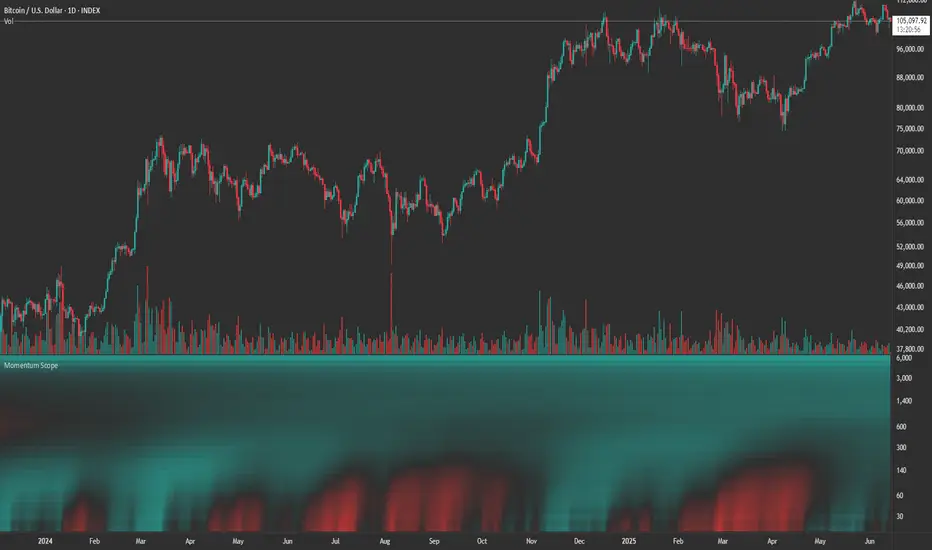
DisplayUtilitiesLibrary "DisplayUtilities"
Display utilities for color management and visual presentation
get_direction_color(direction, up_excessive, up_normal, neutral, down_normal, down_excessive)
Get candle color based on direction and color scheme
Parameters:
direction (int) : Direction value (-2, -1, 0, 1, 2)
up_excessive (color) : Color for +2 direction
up_normal (color) : Color for +1 direction
neutral (color) : Color for 0 direction
down_normal (color) : Color for -1 direction
down_excessive (color) : Color for -2 direction
Returns: Appropriate color for the direction
get_candle_paint_directions(paint_opt, body_dir, bar_dir, breakout_dir, combined_dir)
Get candle directions for different painting algorithms
Parameters:
paint_opt (string) : Painting option algorithm
body_dir (int) : Body direction
bar_dir (int) : Bar direction
breakout_dir (int) : Breakout direction
combined_dir (int) : Combined direction
Returns:
get_bias_paint_directions(paint_bias, unified_dir)
Get paint directions based on bias filter
Parameters:
paint_bias (string) : Paint bias option ("All", "Bull Bias", "Bear Bias")
unified_dir (int) : Unified direction
Returns: Directions for two plotcandle series
get_transparency_levels(sf_filtered, fade_option, fade_opacity)
Calculate transparency levels for strength factor filtering
Parameters:
sf_filtered (bool) : Is strength factor filtered
fade_option (string) : Fade option ("Disabled", "Fade Candle", "Do Not Fade Wick", "Do Not Fade Wick and Border")
fade_opacity (int) : Fade opacity percentage
Returns:
get_strength_factor_filter(filter_option, individual_filters)
Generate strength factor filter conditions
Parameters:
filter_option (string) : Filter option string
individual_filters (map) : Map of individual filter conditions
Returns: Boolean filter result
get_signal_bar_condition(signal_option, individual_filters)
Generate signal bar conditions (inverted filters)
Parameters:
signal_option (string) : Signal bar option string
individual_filters (map) : Map of individual filter conditions
Returns: Boolean signal bar result
get_zscore_signal_condition(z_signal_option, z_filters)
Get Z-score signal bar conditions
Parameters:
z_signal_option (string) : Z-score signal option
z_filters (map) : Map of Z-score filters
Returns: Boolean Z-score signal condition
get_standard_colors()
Create a standard color scheme for directions
Returns: Standard color set
apply_zscore_modification(original_dir, z_filtered)
Modify directions for Z-score excess display
Parameters:
original_dir (int) : Original direction
z_filtered (bool) : Is Z-score filtered (shows excess)
Returns: Modified direction (doubled if excess detected)
get_default_fade_colors()
Get default fade colors for strength factor overlay
Returns: Default colors for TV overlay
should_paint_candles(paint_algo)
Check if paint algorithm should show candles
Parameters:
paint_algo (string) : Paint algorithm option
Returns: True if algorithm should display candles
get_signal_bar_char(signal_type, is_bullish)
Get signal bar character based on signal type
Parameters:
signal_type (string) : Signal type ("strength_factor" or "zscore")
is_bullish (bool) : Direction is bullish
Returns: Character and location for plotchar
get_signal_bar_color(signal_type, is_bullish)
Get signal bar colors
Parameters:
signal_type (string) : Signal type ("strength_factor" or "zscore")
is_bullish (bool) : Direction is bullish
Returns: Signal bar color

Statistical Reliability Index (SRI)Statistical Reliability Index (SRI)
The Statistical Reliability Index (SRI) is a professional financial analysis tool designed to assess the statistical stability and reliability of market conditions. It combines advanced statistical methods to gauge whether current market trends are statistically consistent or prone to erratic behavior. This allows traders to make more informed decisions when navigating trending and choppy markets.
Key Concepts:
1. Extrapolation of Cumulative Distribution Functions (CDF)
What is CDF?
A Cumulative Distribution Function (CDF) is a statistical tool that models the probability of a random variable falling below a certain value.
How it’s used in SRI:
The SRI utilizes the 95th percentile CDF of recent returns to estimate the likelihood of extreme price movements. This helps identify when a market is experiencing statistically significant changes, crucial for forecasting potential breakouts or breakdowns.
Weight in SRI:
The weight of the CDF extrapolation can be adjusted to emphasize its impact on the overall reliability index, allowing customization based on the trader's preference for tail risk analysis.
2. Bias Factor (BF)
What is the Bias Factor?
The Bias Factor measures the ratio of the current market price to the expected mean price calculated over a defined period. It represents the deviation from the typical price level.
How it’s used in SRI:
A higher bias factor indicates that the current price significantly deviates from the historical average, suggesting a potential mean reversion or trend exhaustion.
Weight in SRI:
Adjusting the Bias Factor weight lets users control how much this deviation influences the SRI, balancing between momentum trading and mean reversion strategies.
3. Coefficient of Variation (CV)
What is CV?
The Coefficient of Variation (CV) is a statistical measure that expresses the ratio of the standard deviation to the mean. It indicates the relative variability of asset returns, helping gauge the risk-to-return consistency.
How it’s used in SRI:
A lower CV indicates more stable and predictable price behavior, while a higher CV signals increased volatility. The SRI incorporates the inverse of the normalized CV to reflect price stability positively.
Weight in SRI:
By adjusting the CV weight, users can prioritize consistent price movements over erratic volatility, aligning the indicator with risk tolerance and strategy preferences.
Interpreting the SRI:
1. SRI Plot:
The SRI plot dynamically changes color to reflect market conditions:
Aqua Line: Indicates uptrend stability, signaling statistically consistent upward movements.
Fuchsia Line: Indicates downtrend stability, where statistically reliable downward movements are present.
The overlay background shifts between colors:
Aqua Background: Signifies statistical stability, where trends are historically consistent.
Fuchsia Background: Indicates statistical instability, often associated with trend uncertainty.
Yellow Background: Marks choppy periods, where statistical data suggests that market conditions are not conducive to reliable trading.
2. SRI Volatility Plot:
Displays the volatility of the SRI itself to detect when the indicator is stable or unstable:
Blue Area Fill: Signifies that the SRI is stable, indicating trending conditions.
Yellow Area Fill: Represents choppy or unstable SRI movements, suggesting sideways or unreliable market conditions.
A Chop Threshold Line (dotted yellow) highlights the maximum acceptable SRI volatility before the market is considered too unpredictable.
3. Stability Assessment:
Stable Trend (No Chop):
The SRI is smooth and consistent, often accompanied by aqua or fuchsia lines.
Volatility remains below the chop threshold, indicating a low-risk, trend-following environment.
Chop Mode:
The SRI becomes erratic, and the volatility plot spikes above the threshold.
Marked by a yellow shaded background, indicating uncertain and non-trending conditions.
[Trend Identification:
Use the color-coded SRI line and background to determine uptrend or downtrend reliability.
Be cautious when the SRI volatility plot shows yellow, as this signals trading conditions may not be reliable.
Practical Use Cases:
Trend Confirmation:
Utilize the SRI plot color and background to confirm whether a detected trend is statistically reliable.
Chop Mode Filtering:
During yellow chop periods, it is advisable to reduce trading activity or adopt range-bound strategies.
Strategy Filter:
Combine the SRI with trend-following indicators (like moving averages) to enhance entry and exit accuracy.
Volatility Monitoring:
Pay attention to the SRI volatility plot, as spikes often precede erratic price movements or trend reversals.
Disclaimer:
The Statistical Reliability Index (SRI) is a technical analysis tool designed to aid in market stability assessment and trend validation. It is not intended as a standalone trading signal generator. While the SRI can help identify statistically reliable trends, it is essential to incorporate additional technical and fundamental analysis to make well-informed trading decisions.
Trading and investing involve substantial risk, and past performance does not guarantee future results. Always use risk management practices and consult with a financial advisor to tailor strategies to your individual risk profile and objectives.

Buyers vs SellersBuyers vs Sellers is an indicator which essentially weighs the strength of the buyers against the strength of the sellers. It defines the current relationship between the buyers and the sellers as well as the way that that relationship is changing over time.
User Inputs:
1. Number of Bars To Include In The Calculation - this is the look back period. The amount of past data that is being processed.
2. Length of The ATR - higher values are recommended. This ATR is used as a unit in which the price changes are expressed.
3. Bullish/Bearish Bias Threshold - the minimum value to consider the buyers or the sellers having control of the price.
4. Net Move Average Length - the moving average of the sum of bullish and bearish price changes.
The Calculation Process:
This indicator measures the difference between the opening and the closing prices of each bar in the look back period.
After that it sums together the sizes of the bodies of all the bullish bars and also the sizes of all the bearish bars to create the total bullish price change and total bearish price change for the look back period.
After that it converts the total price changes into percentages of the ATR and divides them by the look back period to get the price change per bar - it is a way of getting the price change values down to less ridiculous numbers regardless of the look back period and while still keeping the proportions intact.
After that it sums the two price changes together to get the net move and performs a simple moving average calculation on it in order to smooth out the values. This is a numerical representation of the relationship between the strength of the bullish and the bearish moves, which is easily readable from the chart.
After that the indicator performs a natural logarithm of the bullish price change divided by the bearish price change. This calculation gives a relationship between the two values which is not tied to the volatility of the instrument, but is expressed purely as a relationship between the strength of one value against the other. The idea is that this would allow for easier comparison across different instruments as the same numbers would represent exactly the same distribution of the strength difference.
The Plotting Logic:
The ATR is plotted as just a number as a reference.
The natural logarithm is presented in two ways.
One way is numerical, to be able to precisely read the value and the colour of the number changes depending if it is positive and above the bias threshold or negative and below the bias threshold.
The other way is in the form of a background colour. It only visualises the bias that can be interpreted based on the logarithm value in relation to the set bias threshold.
The total bullish price change and the total bearish price change are both plotted as a line with the fill between that line and the zero line. This helps visualise the bullish and the bearish moves individually.
The moving average of the sum of the bullish and the bearish moves is added as a line to represent the relationship between the two on a graph and not just as a logarithm.
I hope this indicator will serve you well and help with defining the relationship between the buyers and sellers more objectively, hopefully leading to more profitable trades.
