RSI VWAP v1 [JopAlgo]RSI VWAP v1.1 made stronger by volume-aware!
We know there's nothing new and the original RSI already does an excellent job. We're just working on small, practical improvements – here's our take: The same basic idea, clearer display, and a single, specially developed rolling line: a VWAP of the RSI that incorporates volume (participation) into the calculation.
Do you prefer the pure classic?
You can still use Wilder or Cutler engines –
but the star here is the VW-RSI + rolling line.
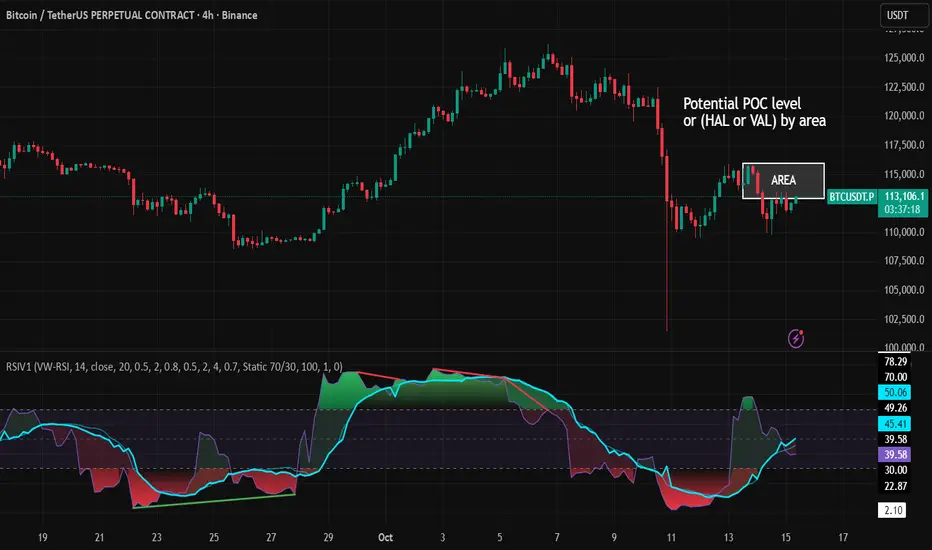
This RSI also offers the possibility of illustrating a possible
POC (Point of Control - or the HAL or VAL) level.
However, the indicator does NOT plot any of these levels itself.
We have included an illustration in the chart for this!
We hope this version makes your decision-making easier.
What you’ll see
The RSI line with a 50 midline and optional bands: either static 70/30 or adaptive μ±k·σ of the Rolling Line.
One smoothing concept only: the Rolling Line (light blue) = VWAP of RSI.
Shadow shading between RSI and the Rolling Line (green when RSI > line, red when RSI < line).
A lighter tint only on the parts of that shadow that sit above the upper band or below the lower band (quick overbought/oversold context).
Simple divergence lines drawn from RSI pivots (green for regular bullish, red for regular bearish). No labels, no buy/sell text—kept deliberately clean.
What’s new, and why it helps
VW-RSI engine (default):
RSI can be computed from volume-weighted up/down moves, so momentum reflects how much traded when price moved—not just the direction.
Rolling Line (VWAP of RSI) with pure VWAP adaptation:
Low volume: blends toward a faster VWAP so early, thin starts aren’t missed.
Volume spikes: blends toward a slower VWAP so a single heavy bar doesn’t whip the curve.
You can reveal the Base Rolling (pre-adaptation) line to see exactly how much adaptation is happening.
Adaptive bands (optional):
Instead of fixed 70/30, use mean ± k·stdev of the Rolling Line over a lookback. Levels breathe with the market—useful in strong trends where static bounds stay pinned.
Minimal, readable panel:
One smoothing, one story. The shadow tells you who’s in control; the lighter highlight shows stretch beyond your lines.
How to read it (fast)
Bias: RSI above 50 (and a rising Rolling Line) → bullish bias; below 50 → bearish bias.
Trigger: RSI crossing the Rolling Line with the bias (e.g., above 50 and crossing up).
Stretch: Near/above the upper band, avoid chasing; near/below the lower band, avoid panic—prefer a cross back through the line.
Divergence lines: Use as context, not as standalone signals. They often help you wait for the next cross or avoid late entries into exhaustion.
Settings that actually matter
RSI Engine: VW-RSI (default), Wilder, or Cutler.
Rolling Line Length: the VWAP length on RSI (higher = calmer, lower = earlier).
Adaptive behavior (pure VWAP):
Speed-up on Low Volume → blends toward fast VWAP (factor of your length).
Dampen Spikes (volume z-score) → blends toward slow VWAP.
Fast/Slow Factors → how far those fast/slow variants sit from the base length.
Bands: choose Static 70/30 or Adaptive μ±k·σ (set the lookback and k).
Visuals: show/hide Base Rolling (ref), main shadow, and highlight beyond bands.
Signal gating: optional “ignore first bars” per day/session if you dislike open noise.
Starter presets
Scalp (1–5m): RSI 9–12, Rolling 12–18, FastFactor ~0.5, SlowFactor ~2.0, Adaptive on.
Intraday (15m–1H): RSI 10–14, Rolling 18–26, Bands k = 1.0–1.4.
Swing (4H–1D): RSI 14–20, Rolling 26–40, Bands k = 1.2–1.8, Adaptive on.
Where it shines (and limits)
Best: liquid markets where volume structure matters (majors, indices, large caps).
Works elsewhere: even with imperfect volume, the shadow + bands remain useful.
Limits: very thin/illiquid assets reduce the benefit of volume-weighting—lengthen settings if needed.
Attribution & License
Based on the concept and baseline implementation of the “Relative Strength Index” by TradingView (Pine v6 built-in).
Released as Open-source (MPL-2.0). Please keep the license header and attribution intact.
Disclaimer
For educational purposes only; not financial advice. Markets carry risk. Test first, use clear levels, and manage risk. This project is independent and not affiliated with or endorsed by TradingView.
Search in scripts for "bias"
MTF Candle Direction Forecast + Breakdown🧭 MTF Candle Direction Forecast + Breakdown 🔥📈🔼
This script is a multi-timeframe (MTF) price action dashboard that helps traders assess real-time directional bias across five customizable timeframes — with a focus on candle behavior, trend alignment, and confidence strength.
📌 What It Does
For each timeframe, this dashboard summarizes:
Current direction → Bullish, Bearish, or Neutral
Confidence score (0–100) → How strongly price is likely to continue in that direction
Candle strength → 🔥 icon appears if the current candle has a large body relative to its range
Trend alignment:
📈 = EMA9 is above EMA20
🔼 = Price is above VWAP
Color-coded background to visually reinforce directional state
Each row gives you a visual “at-a-glance” readout of what price is doing right now — not in the past.
💡 Why It’s Useful
✅ Direction forecasting based on price action
Instead of lagging indicators, this script prioritizes:
Candle body-to-range ratio (momentum)
Real-time VWAP/EMA structure
Immediate price positioning
✅ Confidence is quantified
The score (0–100) helps you judge how reliable each directional signal is:
90+ → Strong conviction
50–70 → Mixed but potentially valid
<40 → Weak move or early signal
✅ Timeframe confluence at a glance
See whether multiple timeframes are aligning directionally — helpful for scalping, day trading, or waiting for multi-timeframe breakout setups.
✅ Visual & intuitive
Icons, colors, and layout make it easy to scan your dashboard instead of deciphering charts or code.
🛠️ Adjustable Settings
Setting Description
Timeframe 1–5 Choose any timeframes to monitor (e.g., 5m, 15m, 1h, 4h)
Candle Display Mode Show trend color via emoji (🟢/🔴) or background shading
Strong Candle Threshold Adjust the body-to-range % needed to trigger 🔥 strength
Bullish/Bearish Background Customize label color coding
Neutral Background (opacity) Set transparency or styling for flat/consolidating zones
Table Location Place the dashboard anywhere on the chart
🎯 Use Cases
Scalpers: Confirm trend across 1m/5m/15m before entering
Day Traders: Use confidence score to avoid low-momentum setups
Swing Traders: Monitor higher timeframes for trend shifts while tracking intraday noise
VWAP/EMA traders: Quickly see when price is reclaiming or losing critical trend levels
🧠 What Makes It Unique?
Unlike generic trend meters or mashups of standard indicators, this script:
Uses live candle dynamics (not just closes or lagging values)
Computes directional bias and confidence together
Visualizes strength and structure in a compact, readable interface
Let’s you filter by price action, not just indicator alignment
💥 Why Traders Love Will Love It
✅ Instant clarity on which timeframes agree
✅ No more guessing candle strength or trend health
✅ Confidence score keeps you out of weak trades
✅ Works with any strategy — trend following, VWAP reclaim, EMA scalps, even breakouts
✅ Keeps your chart clean — all the context, none of the clutter
⚠️ Transparency🧬 Under the Hood
Powered by live candle body analysis, trend structure (EMA9 vs EMA20), and VWAP placement.
All scores are generated in real-time — No repainting or lookahead bias: all values are computed with lookahead=barmerge.lookahead_on
Confidence scores reflect the current candle only — they do not predict future moves but measure momentum and alignment in real-time
Labels update per bar and respond to subtle shifts in candle structure and trend indicators
✅ MTF Trend Snapshot (Live Output Example Shown in Chart Above)
This dashboard gives you a fast, visual summary of market trend and momentum across 5 timeframes. Here's what it's telling you right now:
🕔 5 Minute (5m)
📉 EMA Trend: Down
🔼 Price: Above VWAP
Direction: Bearish (42)
🟥 Weak bearish bias. Short-term pullback against a stronger trend. Use caution — lower confidence and mixed structure.
⏱️ 15 Minute (15m)
📈 EMA Trend: Up
🔼 Price: Above VWAP
Direction: Bullish (73)
🟩 Clean bullish structure with growing momentum. Solid for intraday confirmation.
🕧 30 Minute (30m)
📈 EMA Trend: Up
🔼 Price: Above VWAP
Direction: Bullish (77)
🟩 Stronger trend forming. Above VWAP and EMAs — building conviction.
🕐 1 Hour (1h)
📈 EMA Trend: Up
🔼 Price: Above VWAP
Direction: Bullish (70)
🟩 Confident, clean trend. Good alignment across indicators. Ideal timeframe for swing entries.
🕓 4 Hour (4h)
🔥 Strong Candle
📈 EMA Trend: Up
🔼 Price: Above VWAP
Direction: Bullish (100)
🟩 Full trend alignment with max momentum. Strong body candle + structure — high confidence continuation.
🧠 Quick Takeaway
🔻 5m is pulling back short term
✅ 15m through 4h are fully aligned Bullish
🔥 4h has max confidence — big-picture trend is intact
📈 Ideal setup for momentum traders looking to ride trend with multi-timeframe confirmation
Try pinning this dashboard to your chart during live trading to read price like a story across timeframes, and filter out weak setups with low-confidence noise.

[blackcat] L1 Net Volume DifferenceOVERVIEW
The L1 Net Volume Difference indicator serves as an advanced analytical tool designed to provide traders with deep insights into market sentiment by examining the differential between buying and selling volumes over precise timeframes. By leveraging these volume dynamics, it helps identify trends and potential reversal points more accurately, thereby supporting well-informed decision-making processes. The key focus lies in dissecting intraday changes that reflect short-term market behavior, offering critical input for both swing and day traders alike. 📊
Key benefits encompass:
• Precise calculation of net volume differences grounded in real-time data.
• Interactive visualization elements enhancing interpretability effortlessly.
• Real-time generation of buy/sell signals driven by dynamic volume shifts.
TECHNICAL ANALYSIS COMPONENTS
📉 Volume Accumulation Mechanisms:
Monitors cumulative buy/sell volumes derived from comparative closing prices.
Periodically resets accumulation counters aligning with predefined intervals (e.g., 5-minute bars).
Facilitates identification of directional biases reflecting underlying market forces accurately.
🕵️♂️ Sentiment Detection Algorithms:
Employs proprietary logic distinguishing between bullish/bearish sentiments dynamically.
Ensures consistent adherence to predefined statistical protocols maintaining accuracy.
Supports adaptive thresholds adjusting sensitivities based on changing market conditions flexibly.
🎯 Dynamic Signal Generation:
Detects transitions indicating dominance shifts between buyers/sellers promptly.
Triggers timely alerts enabling swift reactions to evolving market dynamics effectively.
Integrates conditional logic reinforcing signal validity minimizing erroneous activations.
INDICATOR FUNCTIONALITY
🔢 Core Algorithms:
Utilizes moving averages along with standardized deviation formulas generating precise net volume measurements.
Implements Arithmetic Mean Line Algorithm (AMLA) smoothing techniques improving interpretability.
Ensures consistent alignment with established statistical principles preserving fidelity.
🖱️ User Interface Elements:
Dedicated plots displaying real-time net volume markers facilitating swift decision-making.
Context-sensitive color coding distinguishing positive/negative deviations intuitively.
Background shading highlighting proximity to key threshold activations enhancing visibility.
STRATEGY IMPLEMENTATION
✅ Entry Conditions:
Confirm bullish/bearish setups validated through multiple confirmatory signals.
Validate entry decisions considering concurrent market sentiment factors.
Assess alignment between net volume readings and broader trend directions ensuring coherence.
🚫 Exit Mechanisms:
Trigger exits upon hitting predetermined thresholds derived from historical analyses.
Monitor continuous breaches signifying potential trend reversals promptly executing closures.
Execute partial/total closes contingent upon cumulative loss limits preserving capital efficiently.
PARAMETER CONFIGURATIONS
🎯 Optimization Guidelines:
Reset Interval: Governs responsiveness versus stability balancing sensitivity/stability.
Price Source: Dictates primary data series driving volume calculations selecting relevant inputs accurately.
💬 Customization Recommendations:
Commence with baseline defaults; iteratively refine parameters isolating individual impacts.
Evaluate adjustments independently prior to combined modifications minimizing disruptions.
Prioritize minimizing erroneous trigger occurrences first optimizing signal fidelity.
Sustain balanced risk-reward profiles irrespective of chosen settings upholding disciplined approaches.
ADVANCED RISK MANAGEMENT
🛡️ Proactive Risk Mitigation Techniques:
Enforce strict compliance with pre-defined maximum leverage constraints adhering strictly to guidelines.
Mandatorily apply trailing stop-loss orders conforming to script outputs reinforcing discipline.
Allocate positions proportionately relative to available capital reserves managing exposures prudently.
Conduct periodic reviews gauging strategy effectiveness rigorously identifying areas needing refinement.
⚠️ Potential Pitfalls & Solutions:
Address frequent violations arising during heightened volatility phases necessitating manual interventions judiciously.
Manage false alerts warranting immediate attention avoiding adverse consequences systematically.
Prepare contingency plans mitigating margin call possibilities preparing proactive responses effectively.
Continuously assess automated system reliability amidst fluctuating conditions ensuring seamless functionality.
PERFORMANCE AUDITS & REFINEMENTS
🔍 Critical Evaluation Metrics:
Assess win percentages consistently across diverse trading instruments gauging reliability.
Calculate average profit ratios per successful execution measuring profitability efficiency accurately.
Measure peak drawdown durations alongside associated magnitudes evaluating downside risks comprehensively.
Analyze signal generation frequencies revealing hidden patterns potentially skewing outcomes uncovering systematic biases.
📈 Historical Data Analysis Tools:
Maintain comprehensive records capturing every triggered event meticulously documenting results.
Compare realized profits/losses against backtested simulations benchmarking actual vs expected performances accurately.
Identify recurrent systematic errors demanding corrective actions implementing iterative refinements steadily.
Document evolving performance metrics tracking progress dynamically addressing identified shortcomings proactively.
PROBLEM SOLVING ADVICE
🔧 Frequent Encountered Challenges:
Unpredictable behaviors emerging within thinly traded markets requiring filtration processes.
Latency issues manifesting during abrupt price fluctuations causing missed opportunities.
Overfitted models yielding suboptimal results post-extensive tuning demanding recalibrations.
Inaccuracies stemming from incomplete/inaccurate data feeds necessitating verification procedures.
💡 Effective Resolution Pathways:
Exclude low-liquidity assets prone to erratic movements enhancing signal integrity.
Introduce buffer intervals safeguarding major news/event impacts mitigating distortions effectively.
Limit ongoing optimization attempts preventing model degradation maintaining optimal performance levels consistently.
Verify reliable connections ensuring uninterrupted data flows guaranteeing accurate interpretations reliably.
USER ENGAGEMENT SEGMENT
🤝 Community Contributions Welcome
Highly encourage active participation sharing experiences & recommendations!
THANKS
Heartfelt acknowledgment extends to all developers contributing invaluable insights about volume-based trading methodologies! ✨

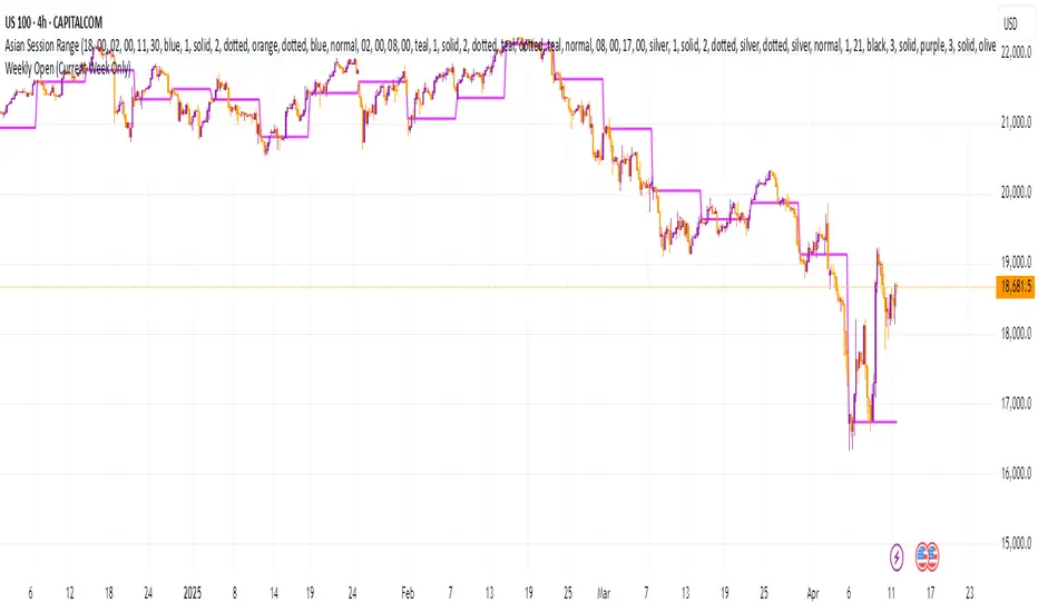
Weekly Open (Current Week Only)📘 Indicator Name: Weekly Open (Current Week Only)
📝 Description:
This indicator plots a horizontal line representing the weekly open price, visible only during the current trading week. At the beginning of each new week (based on TradingView’s weekly time segmentation), the indicator captures the open price of the first candle and draws a constant line across the chart until the week ends. Once the new week begins, the line resets and updates with the new weekly open.
🎯 How to Use – ICT Concepts Integration (Weekly Profile):
This tool is designed to complement ICT (Inner Circle Trader) trading strategies, particularly within the weekly profile framework, by offering a clear and persistent visual of the weekly open, which is a critical reference point in ICT’s market structure theory.
✅ Use Cases:
Directional Bias:
According to ICT concepts, price trading above the weekly open suggests a bullish bias for the week, while trading below it implies bearish conditions.
Traders can use the weekly open line to align their intraweek trades with higher timeframe directional bias.
Dealing Ranges:
Weekly open helps frame the weekly dealing range, especially when combined with other levels like weekly high/low or previous week’s range.
It allows traders to identify potential liquidity pools or areas where price may seek to rebalance.
Mean Reversion Entries:
Price often reverts to or reacts from the weekly open. Traders may use this as a target or entry level, particularly during Monday/Tuesday setups.
Works well in conjunction with concepts like OTE (Optimal Trade Entry) and Judas Swings.
Risk Management:
Acts as a clean and visual anchor to structure stop losses or take-profits based on weekly bias shifts.
Strategy Template - V2This is an educational script created to demonstrate few basic building blocks of a trend based strategy and how to achieve different entry and exit types. My initial intention was to create a comprehensive strategy template which covers all the aspects of strategy. But, ended up creating fully fledged strategy based on trend following.
This is an enhancement on Strategy-Template But this script is comparitively more complex. Hence I decided to create new version instead of updating the existing one.
Lets dive deep.
SIMPLE COMPONENTS OF TREND FOLLOWING STRATEGY
TREND BIAS - This defines the direction of trend. Idea is not to trade against the trend direction. If the bias is bullish, look for long opportunities and if bias is bearish, look for short opportunities. Stay out of the market when the bias is neutral.
Often, trend bias is determined based on longer timeframe conditions. Example - 200 Moving Average, Higher timeframe moving averages, Higher timeframe high-lows etc. can be used for determining the trend bias.
In this script, I am using Weekly donchian channels combined with daily donchian channels to define trend bias.
Long Bias - 40 Day donchian channel sits completely in upper portion of 40 Week dochnial channel.
Short Bias - 40 Day donchian channel sits completely in lower portion of 40 Week donchian channel.
ENTRY CONDITION - Entry signals are generated only in the direction of bias. Hence, when in LongBias, we only get Long signals and when in short bias, we only get short signals.
In our case, when in Long Bias - if price hits 40 day high for the first time, this creates our long entry signal. Similarly when in Short Bias , price hitting 40 day low will create signal for going short. Since we do not take trades opposite to trend, no entry conditions are formed when price hits 40 day high in Short Bias or 40 day low in Long Bias.
EXIT CONDITION - Exit conditions are formed when we get signals of trend failure.
In our case, when in long trade, price hitting 40 day low creates exit signal. Similarly when in short trade price hitting 40 day high creates exit signal for short trade.
DIFFERENT TYPES OF ENTRY AND EXIT
In this script, I have tried to demonstrate different entry and exit types.
Entry types
Market - Enter immediately when entry signal is received. That is, in this case when price crossover over high in long bias and crosses under low in short bias
Stop - This method includes estimating at what level new highs are made and creating a stop buy order at that level. This way, we do not miss if the break out is stronger. But, susciptible to fail during fakeouts.
Limit - This method includes executing a limit order to buy at lower price or sell at higher price. In trend following methods, downside of limit order is when there is genuine breakout, these limit orders may not hit and during trend failures the limit orders are likely to hit and go straight to stop.
Stop-Limit - this is same as stop order but will also place a limit condition to avoid buying on overextended breakout or with lots of slippage.
Exit types
Market - whether to keep the existing trade running or whether to close it is determined after close of each bar and exit orders are executed manually upon receiving exit signal.
Stop - We place stop loss orders beforehand when there is a trade in place. This can help in avoiding big movements against trade within bar. But, this may also stop on false signals or fakeouts.
Take profit
Stop - No take profits are configured.
Target - 30% of the positions are closed when take profit levels are hit. Take profit levels are defined by risk reward.
USING THE CODE AS TEMPLATE
As mentioned earlier, I intended to create a fully fledged strategy template. But, ended up creating a fully fledged stratgy. However, you can take some part of this code and use it to start your own strategy. Will explain what all things can be adopted without worrying about the strategy implementation within
Strategy definition : This can be copied as is and just change the title of strategy. This defines some of the commonly used parameters of strategy which can help with close to realistic backtesting results for your coded strategy and comparison with buy and hold.
Generic Strategy Parameters : The parameter which defines controlling alllowed trade direction and trading window are present here. This again can be copied as is and variable inDateRange can be directly used in entry conditions.
Generic Methods : f_getMovingAverage and f_secureSecurity are handy and can be used as is. atr method provideded by pine gives you ATR based on RMA. If you want SMA or any other moving average based ATR, you can use the method f_getCustomAtr
Trade Statements : This section has all types of trading instructions which includes market/stop/limit/stop-limit type of entries and exits and take profit statements. You can adopt the type of entry you are interested in and change when condition to suit your strategy.
Trade conditions and levels : This section is required. But, cannot be copied. All the trade logic goes here which also sets parameters which are used in when of Trade Statements.
Hope this helps.

Technical Ratings█ OVERVIEW
This indicator calculates TradingView's well-known "Strong Buy", "Buy", "Neutral", "Sell" or "Strong Sell" states using the aggregate biases of 26 different technical indicators.
█ FEATURES
Differences with the built-in version
• You can adjust the weight of the Oscillators and MAs components of the rating here.
• The built-in version produces values matching the states displayed in the "Technicals" ratings gauge; this one does not always, where weighting is used.
• A strategy version is also available as a built-in; this script is an indicator—not a strategy.
• This indicator will show a slightly different vertical scale, as it does not use a fixed scale like the built-in.
• This version allows control over repainting of the signal when you do not use a higher timeframe. Higher timeframe (HTF) information from this version does not repaint.
• You can configure markers on signal breaches of configurable levels, or on advances declines of the signal.
The indicator's settings allow you to:
• Choose the timeframe you want calculations to be made on.
• When not using a HTF, you can select a repainting or non-repainting signal.
• When using both MAs and Oscillators groups to calculate the rating, you can vary the weight of each group in the calculation. The default is 50/50.
Because the MAs group uses longer periods for some of its components, its value is not as jumpy as the Oscillators value.
Increasing the weight of the MAs group will thus have a calming effect on the signal.
• Alerts can be created on the indicator using the conditions configured to control the display of markers.
Display
The calculated rating is displayed as columns, but you can change the style in the inputs. The color of the signal can be one of three colors: bull, bear, or neutral. You can choose from a few presets, or check one and edit its color. The color is determined from the rating's value. Between 0.1 and -0.1 it is in the neutral color. Above/below 0.1/-0.1 it will appear in the bull/bear color. The intensity of the bull/bear color is determined by cumulative advances/declines in the rating. It is capped to 5, so there are five intensities for each of the bull/bear colors.
The "Strong Buy", "Buy", "Neutral", "Sell" or "Strong Sell" state of the last calculated value is displayed to the right of the last bar for each of the three groups: All, MAs and Oscillators. The first value always reflects your selection in the "Rating uses" field and is the one used to display the signal. A "Strong Buy" or "Strong Sell" state appears when the signal is above/below the 0.5/-0.5 level. A "Buy" or "Sell" state appears when the signal is above/below the 0.1/-0.1 level. The "Neutral" state appears when the signal is between 0.1 and -0.1 inclusively.
Five levels are always displayed: 0.5 and 0.1 in the bull color, zero in the neutral color, and -0.1 and - 0.5 in the bull color.
The levels that can be used to determine the breaches displaying long/short markers will only be visible when their respective long/short markers are turned on in the "Direction" input. The levels appear as a bright dotted line in bull/bear colors. You can control both levels separately through the "Longs Level" and "Shorts Level" inputs.
If you specify a higher timeframe that is not greater than the chart's timeframe, an error message will appear and the indicator's background will turn red, as it doesn't make sense to use a lower timeframe than the chart's.
Markers
Markers are small triangles that appear at the bottom and top of the indicator's pane. The marker settings define the conditions that will trigger an alert when you configure an alert on the indicator. You can:
• Choose if you want long, short or both long and short markers.
• Determine the signal level and/or the number of cumulative advances/declines in the signal which must be reached for either a long or short marker to appear.
Reminder: the number of advances/declines is also what controls the brightness of the plotted signal.
• Decide if you want to restrict markers to ones that alternate between longs and shorts, if you are displaying both directions.
This helps to minimize the number of markers, e.g., only the first long marker will be displayed, and then no more long markers will appear until a short comes in, then a long, etc.
Alerts
When you create an alert from this indicator, that alert will trigger whenever your marker conditions are confirmed. Before creating your alert, configure the makers so they reflect the conditions you want your alert to trigger on.
The script uses the alert() function, which entails that you select the "Any alert() function call" condition from the "Create Alert" dialog box when creating alerts on the script. The alert messages can be configured in the inputs. You can safely disregard the warning popup that appears when you create alerts from this script. Alerts will not repaint. Markers will appear, and thus alerts will trigger, at the opening of the bar following the confirmation of the marker condition. Markers will never disappear from the bar once they appear.
Repainting
This indicator uses a two-pronged approach to control repainting. The repainting of the displayed signal is controlled through the "Repainting" field in the script's inputs. This only applies when you have "Same as chart" selected in the "Timeframe" field, as higher timeframe data never repaints. Regardless of that setting, markers and thus alerts never repaint.
When using the chart's timeframe, choosing a non-repainting signal makes the signal one bar late, so that it only displays a value once the bar it was calculated has elapsed. When using a higher timeframe, new values are only displayed once the higher timeframe completes.
Because the markers never repaint, their logic adapts to the repainting setting used for the signal. When the signal repaints, markers will only appear at the close of a realtime bar. When the signal does not repaint (or if you use a higher timeframe), alerts will appear at the beginning of the realtime bar, since they are calculated on values that already do not repaint.
█ CALCULATIONS
The indicator calculates the aggregate value of two groups of indicators: moving averages and oscillators.
The "MAs" group is comprised of 15 different components:
• Six Simple Moving Averages of periods 10, 20, 30, 50, 100 and 200
• Six Exponential Moving Averages of the same periods
• A Hull Moving Average of period 9
• A Volume-weighed Moving Average of period 20
• Ichimoku
The "Oscillators" group includes 11 components:
• RSI
• Stochastic
• CCI
• ADX
• Awesome Oscillator
• Momentum
• MACD
• Stochastic RSI
• Wiliams %R
• Bull Bear Power
• Ultimate Oscillator
The state of each group's components is evaluated to a +1/0/-1 value corresponding to its bull/neutral/bear bias. The resulting value for each of the two groups are then averaged to produce the overall value for the indicator, which oscillates between +1 and -1. The complete conditions used in the calculations are documented in the Help Center .
█ NOTES
Accuracy
When comparing values to the other versions of the Rating, make sure you are comparing similar timeframes, as the "Technicals" gauge in the chart's right pane, for example, uses a 1D timeframe by default.
For coders
We use a handy characteristic of array.avg() which, contrary to avg() , does not return na when one of the averaged values is na . It will average only the array elements which are not na . This is useful in the context where the functions used to calculate the bull/neutral/bear bias for each component used in the rating include special checks to return na whenever the dataset does not yet contain enough data to provide reliable values. This way, components gradually kick in the calculations as the script calculates on more and more historical data.
We also use the new `group` and `tooltip` parameters to input() , as well as dynamic color generation of different transparencies from the bull/bear/neutral colors selected by the user.
Our script was written using the PineCoders Coding Conventions for Pine .
The description was formatted using the techniques explained in the How We Write and Format Script Descriptions PineCoders publication.
Bits and pieces were lifted from the PineCoders' MTF Selection Framework .
Look first. Then leap.

Trend Continuation [OmegaTools]Trend Continuation is a trend-following and trend-continuation tool designed to highlight high-probability pullbacks within an existing directional bias. It helps discretionary and systematic traders visually isolate “continuation zones” where a retracement is more likely to resolve in favor of the prevailing trend rather than trigger a full reversal.
1. Concept and Objective
The indicator combines two key components:
1. A trend bias engine (based either on a Rolling VWAP regime or on swing market structure).
2. A pullback pressure model, which quantifies how deep and “aggressive” the recent retracement has been relative to the trend.
The goal is to identify moments where the market pulls back against the trend, builds enough “reversal pressure,” and then shows signs that the trend is likely to **continue** rather than flip. When specific conditions are met, the indicator highlights bars and plots reference levels that can be used as potential continuation zones, filters, or confluence areas in a broader trading plan.
2. Trend Bias Modes
The primary trend direction is defined through the `Trend Mode` input:
* **RVWAP Mode (default)**
The script computes two rolling volume-weighted average prices over different lengths:
* A **shorter-term rolling VWAP**
* A **longer-term rolling VWAP**
When the shorter RVWAP is above the longer one, the bias is set to **bullish (+1)**. When it is below, the bias is **bearish (-1)**.
This creates a smooth, volume-weighted trend definition that tends to adapt to shifting regimes and filters out minor noise.
* **Market Structure Mode**
In this mode, trend bias is derived from **pivot highs and lows**:
* When price breaks above a recent pivot high, the bias flips to **bullish (+1)**.
* When price breaks below a recent pivot low, the bias flips to **bearish (-1)**.
This approach is more structurally oriented and reacts to significant swing breaks rather than just moving-average style relationships.
If no clear condition is met, the internal bias can temporarily be neutral, though the main design assumes working with clearly bullish or bearish environments.
3. Pullback and Reversal Pressure Logic
Once the trend bias is defined, the indicator measures **pullback intensity** against that trend:
* A **lookback window (“Pullback Length”)** scans recent highs and lows:
* In an uptrend, it tracks the **highest high** over the window and measures how far the current low pulls back from that high.
* In a downtrend, it tracks the **lowest low** and measures how far the current high bounces up from that low.
* This distance is converted into a **“reversal pressure” value**:
* In a bullish bias, deeper pullbacks (lower lows relative to the recent high) indicate stronger counter-trend pressure.
* In a bearish bias, stronger rallies (higher highs relative to the recent low) indicate stronger counter-trend pressure.
The raw reversal pressure is then smoothed with a long-term moving average to separate normal retracements from **statistically significant extremes**.
4. Thresholds and Histogram Coloring
To avoid reacting to every minor pullback, the indicator builds a **dynamic threshold** using a combination of:
* Long-term averages of reversal pressure.
* Standard deviation of reversal pressure.
* High-percentile values of reversal behavior over different sample sizes.
From this, a **threshold line** is derived, and the script then compares the current reversal pressure to this adaptive level:
* The **Reversal Histogram** (column plot) represents the excess reversal pressure above its own long-term average.
* When:
* There is a valid bullish or bearish bias, and
* The histogram is above the dynamic threshold,
the bars of the histogram are **colored**:
* Blue (or a similar “positive” color) in bullish bias.
* Red/pink (or a similar “negative” color) in bearish bias.
* When reversal pressure is below threshold or bias is not relevant, the histogram remains **neutral gray**.
These colored histogram segments represent **“high-tension” pullback states**, where counter-trend pressure has reached an extreme that, historically, often resolves with the original trend continuing rather than fully reversing.
5. Continuation Level and Bar Coloring on Price Chart
To connect the oscillator logic back to the chart:
* A **continuation reference level** is computed on the price series:
* In an uptrend, this is derived by subtracting the threshold from recent highs.
* In a downtrend, it is derived by adding the threshold to recent lows.
* This level is plotted as a **line on the price chart** (only when the trend bias is stable), acting as a visual guide for:
* Potential continuation zones,
* Possible stop-placement or invalidation areas,
* Or filters for entries/exits.
The bars are then **colored** when price crosses or interacts with these levels in the direction of the trend:
* In a bullish bias, bars closing below the continuation level can be highlighted as potential **deep pullback/continuation opportunities** or as warning signals, depending on the user’s playbook.
* In a bearish bias, bars closing above the continuation level are similarly highlighted.
This makes it easy to see where the oscillator’s “extreme pullback” conditions align with structural movements on the actual price bars.
6. Embedded Win-Rate Estimation (WR Table)
The script also includes an internal **win-rate style metric (WR%)** displayed in a small table on the chart:
* It tracks occurrences where:
* A valid bullish or bearish bias is present, and
* The Reversal Histogram is **above the threshold** (i.e., histogram is colored).
* It then approximates the **probability that the trend bias does not change** following such high-pressure pullback events.
* The WR value is shown as a percentage and represents, in essence, the **historical trend-continuation rate** under these specific conditions over the most recent sample of events.
This is not a formal statistical test and does not guarantee future performance, but it provides a quick visual indication of how often these continuation setups have led to **trend persistence** in the recent past.
7. How to Use in Practice
Typical applications include:
Trend-following entries on pullbacks
Identify the main trend using either RVWAP or Market Structure mode.
Wait for a colored histogram bar (reversal pressure above threshold).
Use the continuation reference line and bar coloring on the price chart to refine entry zones or invalidation levels.
Filtering signals from other systems
Run the indicator in the background to confirm trend continuation conditions before taking signals from another strategy (e.g., breakouts or momentum entries).
Only act on long signals when the bias is bullish and a high-pressure pullback has recently occurred; similarly for short signals in bearish conditions.
Risk management and trend monitoring
Monitor when reversal pressure is building against your current position.
Use shifts in bias combined with high reversal pressure to re-evaluate or scale out of trend-following trades.
Recommended steps:
1. Choose your Trend Mode:
- RVWAP for smoother, regime-style trend detection.
- Market Structure for swing-based structural changes.
2. Adjust Trend Length and Pullback Length to match your timeframe (shorter for intraday, longer for swing/position trading).
3. Observe where histogram colors appear and how price reacts around the continuation line and highlighted bars.
4. Integrate these signals into a pre-defined trading plan with clear entry, exit, and risk rules.
8. Limitations and Disclaimer
* This tool is a **technical analysis aid**, not a complete trading system.
* Past behavior of trend continuation or reversal pressure does **not** guarantee future results.
* The embedded WR metric is a **descriptive statistic** based on recent historical conditions only; it is not a promise of performance or a robust statistical forecast.
* All parameters (lengths, thresholds, modes) are user-configurable and should be **tested and validated** on your own data, instruments, and timeframes before any live use.
Disclaimer
This indicator is provided for informational and educational purposes only and does not constitute financial, investment, or trading advice. Trading and investing in financial markets involve substantial risk, including the possible loss of all capital. You are solely responsible for your own trading decisions and for evaluating all information provided by this tool. OmegaTools and the author of this script expressly disclaim any liability for any direct or indirect loss resulting from the use of this indicator. Always consult with a qualified financial professional before making any investment decisions.

Captain Backtest Model [TFO]Created by @imjesstwoone and @mickey1984, this trade model attempts to capture the expansion from the 10:00-14:00 EST 4h candle using just 3 simple steps. All of the information presented in this description has been outlined by its creators, all I did was translate it to Pine Script. All core settings of the trade model may be edited so that users can test several variations, however this description will cover its default, intended behavior using NQ 5m as an example.
Step 1 is to identify our Price Range. In this case, we are concerned with the highest high and the lowest low created from 6:00-10:00 EST.
Step 2 is to wait for either the high or low of said range to be taken out. Whichever side gets taken first determines the long/short bias for the remainder of the Trade Window (i.e. if price takes the range high, bias is long, and vice versa). Bias must be determined by 11:15 EST, otherwise no trades will be taken. This filter is intended to weed out "choppy" trading days.
Step 3 is to wait for a retracement and enter with a close through the previous candle's high (if long biased) or low (if short biased). There are a couple toggleable criteria that we use to define a retracement; one is checking for opposite close candles that indicate a pullback; another is checking if price took the previous candle's low (if long biased) or high (if short biased).
This trade model was initially tested for index futures, particularly ES and NQ, using a 5m chart, however this indicator allows us to backtest any symbol on any timeframe. Creators @imjesstwoone and @mickey1984 specified a 5 point stop loss on ES and a 25 point stop loss on NQ with their testing.
I've personally found some success in backtesting NQ 5m using a 25 point stop loss and 75 point profit target (3:1 R). Enabling the Use Fixed R:R parameter will ensure that these stops and targets are utilized, otherwise it will enter and hold the position until the close of the Trade Window.

Backtesting & Trading Engine [PineCoders]The PineCoders Backtesting and Trading Engine is a sophisticated framework with hybrid code that can run as a study to generate alerts for automated or discretionary trading while simultaneously providing backtest results. It can also easily be converted to a TradingView strategy in order to run TV backtesting. The Engine comes with many built-in strats for entries, filters, stops and exits, but you can also add you own.
If, like any self-respecting strategy modeler should, you spend a reasonable amount of time constantly researching new strategies and tinkering, our hope is that the Engine will become your inseparable go-to tool to test the validity of your creations, as once your tests are conclusive, you will be able to run this code as a study to generate the alerts required to put it in real-world use, whether for discretionary trading or to interface with an execution bot/app. You may also find the backtesting results the Engine produces in study mode enough for your needs and spend most of your time there, only occasionally converting to strategy mode in order to backtest using TV backtesting.
As you will quickly grasp when you bring up this script’s Settings, this is a complex tool. While you will be able to see results very quickly by just putting it on a chart and using its built-in strategies, in order to reap the full benefits of the PineCoders Engine, you will need to invest the time required to understand the subtleties involved in putting all its potential into play.
Disclaimer: use the Engine at your own risk.
Before we delve in more detail, here’s a bird’s eye view of the Engine’s features:
More than 40 built-in strategies,
Customizable components,
Coupling with your own external indicator,
Simple conversion from Study to Strategy modes,
Post-Exit analysis to search for alternate trade outcomes,
Use of the Data Window to show detailed bar by bar trade information and global statistics, including some not provided by TV backtesting,
Plotting of reminders and generation of alerts on in-trade events.
By combining your own strats to the built-in strats supplied with the Engine, and then tuning the numerous options and parameters in the Inputs dialog box, you will be able to play what-if scenarios from an infinite number of permutations.
USE CASES
You have written an indicator that provides an entry strat but it’s missing other components like a filter and a stop strategy. You add a plot in your indicator that respects the Engine’s External Signal Protocol, connect it to the Engine by simply selecting your indicator’s plot name in the Engine’s Settings/Inputs and then run tests on different combinations of entry stops, in-trade stops and profit taking strats to find out which one produces the best results with your entry strat.
You are building a complex strategy that you will want to run as an indicator generating alerts to be sent to a third-party execution bot. You insert your code in the Engine’s modules and leverage its trade management code to quickly move your strategy into production.
You have many different filters and want to explore results using them separately or in combination. Integrate the filter code in the Engine and run through different permutations or hook up your filtering through the external input and control your filter combos from your indicator.
You are tweaking the parameters of your entry, filter or stop strat. You integrate it in the Engine and evaluate its performance using the Engine’s statistics.
You always wondered what results a random entry strat would yield on your markets. You use the Engine’s built-in random entry strat and test it using different combinations of filters, stop and exit strats.
You want to evaluate the impact of fees and slippage on your strategy. You use the Engine’s inputs to play with different values and get immediate feedback in the detailed numbers provided in the Data Window.
You just want to inspect the individual trades your strategy generates. You include it in the Engine and then inspect trades visually on your charts, looking at the numbers in the Data Window as you move your cursor around.
You have never written a production-grade strategy and you want to learn how. Inspect the code in the Engine; you will find essential components typical of what is being used in actual trading systems.
You have run your system for a while and have compiled actual slippage information and your broker/exchange has updated his fees schedule. You enter the information in the Engine and run it on your markets to see the impact this has on your results.
FEATURES
Before going into the detail of the Inputs and the Data Window numbers, here’s a more detailed overview of the Engine’s features.
Built-in strats
The engine comes with more than 40 pre-coded strategies for the following standard system components:
Entries,
Filters,
Entry stops,
2 stage in-trade stops with kick-in rules,
Pyramiding rules,
Hard exits.
While some of the filter and stop strats provided may be useful in production-quality systems, you will not devise crazy profit-generating systems using only the entry strats supplied; that part is still up to you, as will be finding the elusive combination of components that makes winning systems. The Engine will, however, provide you with a solid foundation where all the trade management nitty-gritty is handled for you. By binding your custom strats to the Engine, you will be able to build reliable systems of the best quality currently allowed on the TV platform.
On-chart trade information
As you move over the bars in a trade, you will see trade numbers in the Data Window change at each bar. The engine calculates the P&L at every bar, including slippage and fees that would be incurred were the trade exited at that bar’s close. If the trade includes pyramided entries, those will be taken into account as well, although for those, final fees and slippage are only calculated at the trade’s exit.
You can also see on-chart markers for the entry level, stop positions, in-trade special events and entries/exits (you will want to disable these when using the Engine in strategy mode to see TV backtesting results).
Customization
You can couple your own strats to the Engine in two ways:
1. By inserting your own code in the Engine’s different modules. The modular design should enable you to do so with minimal effort by following the instructions in the code.
2. By linking an external indicator to the engine. After making the proper selections in the engine’s Settings and providing values respecting the engine’s protocol, your external indicator can, when the Engine is used in Indicator mode only:
Tell the engine when to enter long or short trades, but let the engine’s in-trade stop and exit strats manage the exits,
Signal both entries and exits,
Provide an entry stop along with your entry signal,
Filter other entry signals generated by any of the engine’s entry strats.
Conversion from strategy to study
TradingView strategies are required to backtest using the TradingView backtesting feature, but if you want to generate alerts with your script, whether for automated trading or just to trigger alerts that you will use in discretionary trading, your code has to run as a study since, for the time being, strategies can’t generate alerts. From hereon we will use indicator as a synonym for study.
Unless you want to maintain two code bases, you will need hybrid code that easily flips between strategy and indicator modes, and your code will need to restrict its use of strategy() calls and their arguments if it’s going to be able to run both as an indicator and a strategy using the same trade logic. That’s one of the benefits of using this Engine. Once you will have entered your own strats in the Engine, it will be a matter of commenting/uncommenting only four lines of code to flip between indicator and strategy modes in a matter of seconds.
Additionally, even when running in Indicator mode, the Engine will still provide you with precious numbers on your individual trades and global results, some of which are not available with normal TradingView backtesting.
Post-Exit Analysis for alternate outcomes (PEA)
While typical backtesting shows results of trade outcomes, PEA focuses on what could have happened after the exit. The intention is to help traders get an idea of the opportunity/risk in the bars following the trade in order to evaluate if their exit strategies are too aggressive or conservative.
After a trade is exited, the Engine’s PEA module continues analyzing outcomes for a user-defined quantity of bars. It identifies the maximum opportunity and risk available in that space, and calculates the drawdown required to reach the highest opportunity level post-exit, while recording the number of bars to that point.
Typically, if you can’t find opportunity greater than 1X past your trade using a few different reasonable lengths of PEA, your strategy is doing pretty good at capturing opportunity. Remember that 100% of opportunity is never capturable. If, however, PEA was finding post-trade maximum opportunity of 3 or 4X with average drawdowns of 0.3 to those areas, this could be a clue revealing your system is exiting trades prematurely. To analyze PEA numbers, you can uncomment complete sets of plots in the Plot module to reveal detailed global and individual PEA numbers.
Statistics
The Engine provides stats on your trades that TV backtesting does not provide, such as:
Average Profitability Per Trade (APPT), aka statistical expectancy, a crucial value.
APPT per bar,
Average stop size,
Traded volume .
It also shows you on a trade-by-trade basis, on-going individual trade results and data.
In-trade events
In-trade events can plot reminders and trigger alerts when they occur. The built-in events are:
Price approaching stop,
Possible tops/bottoms,
Large stop movement (for discretionary trading where stop is moved manually),
Large price movements.
Slippage and Fees
Even when running in indicator mode, the Engine allows for slippage and fees to be included in the logic and test results.
Alerts
The alert creation mechanism allows you to configure alerts on any combination of the normal or pyramided entries, exits and in-trade events.
Backtesting results
A few words on the numbers calculated in the Engine. Priority is given to numbers not shown in TV backtesting, as you can readily convert the script to a strategy if you need them.
We have chosen to focus on numbers expressing results relative to X (the trade’s risk) rather than in absolute currency numbers or in other more conventional but less useful ways. For example, most of the individual trade results are not shown in percentages, as this unit of measure is often less meaningful than those expressed in units of risk (X). A trade that closes with a +25% result, for example, is a poor outcome if it was entered with a -50% stop. Expressed in X, this trade’s P&L becomes 0.5, which provides much better insight into the trade’s outcome. A trade that closes with a P&L of +2X has earned twice the risk incurred upon entry, which would represent a pre-trade risk:reward ratio of 2.
The way to go about it when you think in X’s and that you adopt the sound risk management policy to risk a fixed percentage of your account on each trade is to equate a currency value to a unit of X. E.g. your account is 10K USD and you decide you will risk a maximum of 1% of it on each trade. That means your unit of X for each trade is worth 100 USD. If your APPT is 2X, this means every time you risk 100 USD in a trade, you can expect to make, on average, 200 USD.
By presenting results this way, we hope that the Engine’s statistics will appeal to those cognisant of sound risk management strategies, while gently leading traders who aren’t, towards them.
We trade to turn in tangible profits of course, so at some point currency must come into play. Accordingly, some values such as equity, P&L, slippage and fees are expressed in currency.
Many of the usual numbers shown in TV backtests are nonetheless available, but they have been commented out in the Engine’s Plot module.
Position sizing and risk management
All good system designers understand that optimal risk management is at the very heart of all winning strategies. The risk in a trade is defined by the fraction of current equity represented by the amplitude of the stop, so in order to manage risk optimally on each trade, position size should adjust to the stop’s amplitude. Systems that enter trades with a fixed stop amplitude can get away with calculating position size as a fixed percentage of current equity. In the context of a test run where equity varies, what represents a fixed amount of risk translates into different currency values.
Dynamically adjusting position size throughout a system’s life is optimal in many ways. First, as position sizing will vary with current equity, it reproduces a behavioral pattern common to experienced traders, who will dial down risk when confronted to poor performance and increase it when performance improves. Second, limiting risk confers more predictability to statistical test results. Third, position sizing isn’t just about managing risk, it’s also about maximizing opportunity. By using the maximum leverage (no reference to trading on margin here) into the trade that your risk management strategy allows, a dynamic position size allows you to capture maximal opportunity.
To calculate position sizes using the fixed risk method, we use the following formula: Position = Account * MaxRisk% / Stop% [, which calculates a position size taking into account the trade’s entry stop so that if the trade is stopped out, 100 USD will be lost. For someone who manages risk this way, common instructions to invest a certain percentage of your account in a position are simply worthless, as they do not take into account the risk incurred in the trade.
The Engine lets you select either the fixed risk or fixed percentage of equity position sizing methods. The closest thing to dynamic position sizing that can currently be done with alerts is to use a bot that allows syntax to specify position size as a percentage of equity which, while being dynamic in the sense that it will adapt to current equity when the trade is entered, does not allow us to modulate position size using the stop’s amplitude. Changes to alerts are on the way which should solve this problem.
In order for you to simulate performance with the constraint of fixed position sizing, the Engine also offers a third, less preferable option, where position size is defined as a fixed percentage of initial capital so that it is constant throughout the test and will thus represent a varying proportion of current equity.
Let’s recap. The three position sizing methods the Engine offers are:
1. By specifying the maximum percentage of risk to incur on your remaining equity, so the Engine will dynamically adjust position size for each trade so that, combining the stop’s amplitude with position size will yield a fixed percentage of risk incurred on current equity,
2. By specifying a fixed percentage of remaining equity. Note that unless your system has a fixed stop at entry, this method will not provide maximal risk control, as risk will vary with the amplitude of the stop for every trade. This method, as the first, does however have the advantage of automatically adjusting position size to equity. It is the Engine’s default method because it has an equivalent in TV backtesting, so when flipping between indicator and strategy mode, test results will more or less correspond.
3. By specifying a fixed percentage of the Initial Capital. While this is the least preferable method, it nonetheless reflects the reality confronted by most system designers on TradingView today. In this case, risk varies both because the fixed position size in initial capital currency represents a varying percentage of remaining equity, and because the trade’s stop amplitude may vary, adding another variability vector to risk.
Note that the Engine cannot display equity results for strategies entering trades for a fixed amount of shares/contracts at a variable price.
SETTINGS/INPUTS
Because the initial text first published with a script cannot be edited later and because there are just too many options, the Engine’s Inputs will not be covered in minute detail, as they will most certainly evolve. We will go over them with broad strokes; you should be able to figure the rest out. If you have questions, just ask them here or in the PineCoders Telegram group.
Display
The display header’s checkbox does nothing.
For the moment, only one exit strategy uses a take profit level, so only that one will show information when checking “Show Take Profit Level”.
Entries
You can activate two simultaneous entry strats, each selected from the same set of strats contained in the Engine. If you select two and they fire simultaneously, the main strat’s signal will be used.
The random strat in each list uses a different seed, so you will get different results from each.
The “Filter transitions” and “Filter states” strats delegate signal generation to the selected filter(s). “Filter transitions” signals will only fire when the filter transitions into bull/bear state, so after a trade is stopped out, the next entry may take some time to trigger if the filter’s state does not change quickly. When you choose “Filter states”, then a new trade will be entered immediately after an exit in the direction the filter allows.
If you select “External Indicator”, your indicator will need to generate a +2/-2 (or a positive/negative stop value) to enter a long/short position, providing the selected filters allow for it. If you wish to use the Engine’s capacity to also derive the entry stop level from your indicator’s signal, then you must explicitly choose this option in the Entry Stops section.
Filters
You can activate as many filters as you wish; they are additive. The “Maximum stop allowed on entry” is an important component of proper risk management. If your system has an average 3% stop size and you need to trade using fixed position sizes because of alert/execution bot limitations, you must use this filter because if your system was to enter a trade with a 15% stop, that trade would incur 5 times the normal risk, and its result would account for an abnormally high proportion in your system’s performance.
Remember that any filter can also be used as an entry signal, either when it changes states, or whenever no trade is active and the filter is in a bull or bear mode.
Entry Stops
An entry stop must be selected in the Engine, as it requires a stop level before the in-trade stop is calculated. Until the selected in-trade stop strat generates a stop that comes closer to price than the entry stop (or respects another one of the in-trade stops kick in strats), the entry stop level is used.
It is here that you must select “External Indicator” if your indicator supplies a +price/-price value to be used as the entry stop. A +price is expected for a long entry and a -price value will enter a short with a stop at price. Note that the price is the absolute price, not an offset to the current price level.
In-Trade Stops
The Engine comes with many built-in in-trade stop strats. Note that some of them share the “Length” and “Multiple” field, so when you swap between them, be sure that the length and multiple in use correspond to what you want for that stop strat. Suggested defaults appear with the name of each strat in the dropdown.
In addition to the strat you wish to use, you must also determine when it kicks in to replace the initial entry’s stop, which is determined using different strats. For strats where you can define a positive or negative multiple of X, percentage or fixed value for a kick-in strat, a positive value is above the trade’s entry fill and a negative one below. A value of zero represents breakeven.
Pyramiding
What you specify in this section are the rules that allow pyramiding to happen. By themselves, these rules will not generate pyramiding entries. For those to happen, entry signals must be issued by one of the active entry strats, and conform to the pyramiding rules which act as a filter for them. The “Filter must allow entry” selection must be chosen if you want the usual system’s filters to act as additional filtering criteria for your pyramided entries.
Hard Exits
You can choose from a variety of hard exit strats. Hard exits are exit strategies which signal trade exits on specific events, as opposed to price breaching a stop level in In-Trade Stops strategies. They are self-explanatory. The last one labelled When Take Profit Level (multiple of X) is reached is the only one that uses a level, but contrary to stops, it is above price and while it is relative because it is expressed as a multiple of X, it does not move during the trade. This is the level called Take Profit that is show when the “Show Take Profit Level” checkbox is checked in the Display section.
While stops focus on managing risk, hard exit strategies try to put the emphasis on capturing opportunity.
Slippage
You can define it as a percentage or a fixed value, with different settings for entries and exits. The entry and exit markers on the chart show the impact of slippage on the entry price (the fill).
Fees
Fees, whether expressed as a percentage of position size in and out of the trade or as a fixed value per in and out, are in the same units of currency as the capital defined in the Position Sizing section. Fees being deducted from your Capital, they do not have an impact on the chart marker positions.
In-Trade Events
These events will only trigger during trades. They can be helpful to act as reminders for traders using the Engine as assistance to discretionary trading.
Post-Exit Analysis
It is normally on. Some of its results will show in the Global Numbers section of the Data Window. Only a few of the statistics generated are shown; many more are available, but commented out in the Plot module.
Date Range Filtering
Note that you don’t have to change the dates to enable/diable filtering. When you are done with a specific date range, just uncheck “Date Range Filtering” to disable date filtering.
Alert Triggers
Each selection corresponds to one condition. Conditions can be combined into a single alert as you please. Just be sure you have selected the ones you want to trigger the alert before you create the alert. For example, if you trade in both directions and you want a single alert to trigger on both types of exits, you must select both “Long Exit” and “Short Exit” before creating your alert.
Once the alert is triggered, these settings no longer have relevance as they have been saved with the alert.
When viewing charts where an alert has just triggered, if your alert triggers on more than one condition, you will need the appropriate markers active on your chart to figure out which condition triggered the alert, since plotting of markers is independent of alert management.
Position sizing
You have 3 options to determine position size:
1. Proportional to Stop -> Variable, with a cap on size.
2. Percentage of equity -> Variable.
3. Percentage of Initial Capital -> Fixed.
External Indicator
This is where you connect your indicator’s plot that will generate the signals the Engine will act upon. Remember this only works in Indicator mode.
DATA WINDOW INFORMATION
The top part of the window contains global numbers while the individual trade information appears in the bottom part. The different types of units used to express values are:
curr: denotes the currency used in the Position Sizing section of Inputs for the Initial Capital value.
quote: denotes quote currency, i.e. the value the instrument is expressed in, or the right side of the market pair (USD in EURUSD ).
X: the stop’s amplitude, itself expressed in quote currency, which we use to express a trade’s P&L, so that a trade with P&L=2X has made twice the stop’s amplitude in profit. This is sometimes referred to as R, since it represents one unit of risk. It is also the unit of measure used in the APPT, which denotes expected reward per unit of risk.
X%: is also the stop’s amplitude, but expressed as a percentage of the Entry Fill.
The numbers appearing in the Data Window are all prefixed:
“ALL:” the number is the average for all first entries and pyramided entries.
”1ST:” the number is for first entries only.
”PYR:” the number is for pyramided entries only.
”PEA:” the number is for Post-Exit Analyses
Global Numbers
Numbers in this section represent the results of all trades up to the cursor on the chart.
Average Profitability Per Trade (X): This value is the most important gauge of your strat’s worthiness. It represents the returns that can be expected from your strat for each unit of risk incurred. E.g.: your APPT is 2.0, thus for every unit of currency you invest in a trade, you can on average expect to obtain 2 after the trade. APPT is also referred to as “statistical expectancy”. If it is negative, your strategy is losing, even if your win rate is very good (it means your winning trades aren’t winning enough, or your losing trades lose too much, or both). Its counterpart in currency is also shown, as is the APPT/bar, which can be a useful gauge in deciding between rivalling systems.
Profit Factor: Gross of winning trades/Gross of losing trades. Strategy is profitable when >1. Not as useful as the APPT because it doesn’t take into account the win rate and the average win/loss per trade. It is calculated from the total winning/losing results of this particular backtest and has less predictive value than the APPT. A good profit factor together with a poor APPT means you just found a chart where your system outperformed. Relying too much on the profit factor is a bit like a poker player who would think going all in with two’s against aces is optimal because he just won a hand that way.
Win Rate: Percentage of winning trades out of all trades. Taken alone, it doesn’t have much to do with strategy profitability. You can have a win rate of 99% but if that one trade in 100 ruins you because of poor risk management, 99% doesn’t look so good anymore. This number speaks more of the system’s profile than its worthiness. Still, it can be useful to gauge if the system fits your personality. It can also be useful to traders intending to sell their systems, as low win rate systems are more difficult to sell and require more handholding of worried customers.
Equity (curr): This the sum of initial capital and the P&L of your system’s trades, including fees and slippage.
Return on Capital is the equivalent of TV’s Net Profit figure, i.e. the variation on your initial capital.
Maximum drawdown is the maximal drawdown from the highest equity point until the drop . There is also a close to close (meaning it doesn’t take into account in-trade variations) maximum drawdown value commented out in the code.
The next values are self-explanatory, until:
PYR: Avg Profitability Per Entry (X): this is the APPT for all pyramided entries.
PEA: Avg Max Opp . Available (X): the average maximal opportunity found in the Post-Exit Analyses.
PEA: Avg Drawdown to Max Opp . (X): this represents the maximum drawdown (incurred from the close at the beginning of the PEA analysis) required to reach the maximal opportunity point.
Trade Information
Numbers in this section concern only the current trade under the cursor. Most of them are self-explanatory. Use the description’s prefix to determine what the values applies to.
PYR: Avg Profitability Per Entry (X): While this value includes the impact of all current pyramided entries (and only those) and updates when you move your cursor around, P&L only reflects fees at the trade’s last bar.
PEA: Max Opp . Available (X): It’s the most profitable close reached post-trade, measured from the trade’s Exit Fill, expressed in the X value of the trade the PEA follows.
PEA: Drawdown to Max Opp . (X): This is the maximum drawdown from the trade’s Exit Fill that needs to be sustained in order to reach the maximum opportunity point, also expressed in X. Note that PEA numbers do not include slippage and fees.
EXTERNAL SIGNAL PROTOCOL
Only one external indicator can be connected to a script; in order to leverage its use to the fullest, the engine provides options to use it as either an entry signal, an entry/exit signal or a filter. When used as an entry signal, you can also use the signal to provide the entry’s stop. Here’s how this works:
For filter state: supply +1 for bull (long entries allowed), -1 for bear (short entries allowed).
For entry signals: supply +2 for long, -2 for short.
For exit signals: supply +3 for exit from long, -3 for exit from short.
To send an entry stop level with an entry signal: Send positive stop level for long entry (e.g. 103.33 to enter a long with a stop at 103.33), negative stop level for short entry (e.g. -103.33 to enter a short with a stop at 103.33). If you use this feature, your indicator will have to check for exact stop levels of 1.0, 2.0 or 3.0 and their negative counterparts, and fudge them with a tick in order to avoid confusion with other signals in the protocol.
Remember that mere generation of the values by your indicator will have no effect until you explicitly allow their use in the appropriate sections of the Engine’s Settings/Inputs.
An example of a script issuing a signal for the Engine is published by PineCoders.
RECOMMENDATIONS TO ASPIRING SYSTEM DESIGNERS
Stick to higher timeframes. On progressively lower timeframes, margins decrease and fees and slippage take a proportionally larger portion of profits, to the point where they can very easily turn a profitable strategy into a losing one. Additionally, your margin for error shrinks as the equilibrium of your system’s profitability becomes more fragile with the tight numbers involved in the shorter time frames. Avoid <1H time frames.
Know and calculate fees and slippage. To avoid market shock, backtest using conservative fees and slippage parameters. Systems rarely show unexpectedly good returns when they are confronted to the markets, so put all chances on your side by being outrageously conservative—or a the very least, realistic. Test results that do not include fees and slippage are worthless. Slippage is there for a reason, and that’s because our interventions in the market change the market. It is easier to find alpha in illiquid markets such as cryptos because not many large players participate in them. If your backtesting results are based on moving large positions and you don’t also add the inevitable slippage that will occur when you enter/exit thin markets, your backtesting will produce unrealistic results. Even if you do include large slippage in your settings, the Engine can only do so much as it will not let slippage push fills past the high or low of the entry bar, but the gap may be much larger in illiquid markets.
Never test and optimize your system on the same dataset , as that is the perfect recipe for overfitting or data dredging, which is trying to find one precise set of rules/parameters that works only on one dataset. These setups are the most fragile and often get destroyed when they meet the real world.
Try to find datasets yielding more than 100 trades. Less than that and results are not as reliable.
Consider all backtesting results with suspicion. If you never entertained sceptic tendencies, now is the time to begin. If your backtest results look really good, assume they are flawed, either because of your methodology, the data you’re using or the software doing the testing. Always assume the worse and learn proper backtesting techniques such as monte carlo simulations and walk forward analysis to avoid the traps and biases that unchecked greed will set for you. If you are not familiar with concepts such as survivor bias, lookahead bias and confirmation bias, learn about them.
Stick to simple bars or candles when designing systems. Other types of bars often do not yield reliable results, whether by design (Heikin Ashi) or because of the way they are implemented on TV (Renko bars).
Know that you don’t know and use that knowledge to learn more about systems and how to properly test them, about your biases, and about yourself.
Manage risk first , then capture opportunity.
Respect the inherent uncertainty of the future. Cleanse yourself of the sad arrogance and unchecked greed common to newcomers to trading. Strive for rationality. Respect the fact that while backtest results may look promising, there is no guarantee they will repeat in the future (there is actually a high probability they won’t!), because the future is fundamentally unknowable. If you develop a system that looks promising, don’t oversell it to others whose greed may lead them to entertain unreasonable expectations.
Have a plan. Understand what king of trading system you are trying to build. Have a clear picture or where entries, exits and other important levels will be in the sort of trade you are trying to create with your system. This stated direction will help you discard more efficiently many of the inevitably useless ideas that will pop up during system design.
Be wary of complexity. Experienced systems engineers understand how rapidly complexity builds when you assemble components together—however simple each one may be. The more complex your system, the more difficult it will be to manage.
Play! . Allow yourself time to play around when you design your systems. While much comes about from working with a purpose, great ideas sometimes come out of just trying things with no set goal, when you are stuck and don’t know how to move ahead. Have fun!
@LucF
NOTES
While the engine’s code can supply multiple consecutive entries of longs or shorts in order to scale positions (pyramid), all exits currently assume the execution bot will exit the totality of the position. No partial exits are currently possible with the Engine.
Because the Engine is literally crippled by the limitations on the number of plots a script can output on TV; it can only show a fraction of all the information it calculates in the Data Window. You will find in the Plot Module vast amounts of commented out lines that you can activate if you also disable an equivalent number of other plots. This may be useful to explore certain characteristics of your system in more detail.
When backtesting using the TV backtesting feature, you will need to provide the strategy parameters you wish to use through either Settings/Properties or by changing the default values in the code’s header. These values are defined in variables and used not only in the strategy() statement, but also as defaults in the Engine’s relevant Inputs.
If you want to test using pyramiding, then both the strategy’s Setting/Properties and the Engine’s Settings/Inputs need to allow pyramiding.
If you find any bugs in the Engine, please let us know.
THANKS
To @glaz for allowing the use of his unpublished MA Squize in the filters.
To @everget for his Chandelier stop code, which is also used as a filter in the Engine.
To @RicardoSantos for his pseudo-random generator, and because it’s from him that I first read in the Pine chat about the idea of using an external indicator as input into another. In the PineCoders group, @theheirophant then mentioned the idea of using it as a buy/sell signal and @simpelyfe showed a piece of code implementing the idea. That’s the tortuous story behind the use of the external indicator in the Engine.
To @admin for the Volatility stop’s original code and for the donchian function lifted from Ichimoku .
To @BobHoward21 for the v3 version of Volatility Stop .
To @scarf and @midtownsk8rguy for the color tuning.
To many other scripters who provided encouragement and suggestions for improvement during the long process of writing and testing this piece of code.
To J. Welles Wilder Jr. for ATR, used extensively throughout the Engine.
To TradingView for graciously making an account available to PineCoders.
And finally, to all fellow PineCoders for the constant intellectual stimulation; it is a privilege to share ideas with you all. The Engine is for all TradingView PineCoders, of course—but especially for you.
Look first. Then leap.
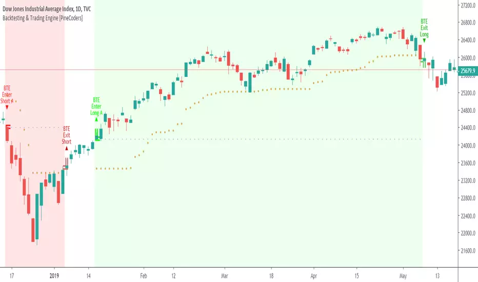
QQE MT4 [JOY]I have taken Glaz's code from and converted to V6 to ensure we have the latest version.
Smoothed RSI (yellow) via EMA with configurable period; serves as the main signal line.
ATR of the smoothed RSI is double‑smoothed with a Wilder lookback (RSI2−1) and scaled by the QQE multiplier to form dynamic bands.
Slow trailing stop (red) tracks the smoothed RSI; trend flips when smoothed RSI crosses the opposite band.
How to use it?
* Trend bias: red line below yellow = bullish bias; red above yellow = bearish bias.
* Crossovers: bullish when smoothed RSI crosses above the red trailing stop; bearish on the opposite cross.
* Works best on volatile pairs as in the original description; test and tune the multiplier and smoothing for your market/timeframe.
* Because it’s derived from an oscillator, signals are on RSI scale, not price; overlays will not show price-level stops.

Dynamic Equity Allocation Model"Cash is Trash"? Not Always. Here's Why Science Beats Guesswork.
Every retail trader knows the frustration: you draw support and resistance lines, you spot patterns, you follow market gurus on social media—and still, when the next bear market hits, your portfolio bleeds red. Meanwhile, institutional investors seem to navigate market turbulence with ease, preserving capital when markets crash and participating when they rally. What's their secret?
The answer isn't insider information or access to exotic derivatives. It's systematic, scientifically validated decision-making. While most retail traders rely on subjective chart analysis and emotional reactions, professional portfolio managers use quantitative models that remove emotion from the equation and process multiple streams of market information simultaneously.
This document presents exactly such a system—not a proprietary black box available only to hedge funds, but a fully transparent, academically grounded framework that any serious investor can understand and apply. The Dynamic Equity Allocation Model (DEAM) synthesizes decades of financial research from Nobel laureates and leading academics into a practical tool for tactical asset allocation.
Stop drawing colorful lines on your chart and start thinking like a quant. This isn't about predicting where the market goes next week—it's about systematically adjusting your risk exposure based on what the data actually tells you. When valuations scream danger, when volatility spikes, when credit markets freeze, when multiple warning signals align—that's when cash isn't trash. That's when cash saves your portfolio.
The irony of "cash is trash" rhetoric is that it ignores timing. Yes, being 100% cash for decades would be disastrous. But being 100% equities through every crisis is equally foolish. The sophisticated approach is dynamic: aggressive when conditions favor risk-taking, defensive when they don't. This model shows you how to make that decision systematically, not emotionally.
Whether you're managing your own retirement portfolio or seeking to understand how institutional allocation strategies work, this comprehensive analysis provides the theoretical foundation, mathematical implementation, and practical guidance to elevate your investment approach from amateur to professional.
The choice is yours: keep hoping your chart patterns work out, or start using the same quantitative methods that professionals rely on. The tools are here. The research is cited. The methodology is explained. All you need to do is read, understand, and apply.
The Dynamic Equity Allocation Model (DEAM) is a quantitative framework for systematic allocation between equities and cash, grounded in modern portfolio theory and empirical market research. The model integrates five scientifically validated dimensions of market analysis—market regime, risk metrics, valuation, sentiment, and macroeconomic conditions—to generate dynamic allocation recommendations ranging from 0% to 100% equity exposure. This work documents the theoretical foundations, mathematical implementation, and practical application of this multi-factor approach.
1. Introduction and Theoretical Background
1.1 The Limitations of Static Portfolio Allocation
Traditional portfolio theory, as formulated by Markowitz (1952) in his seminal work "Portfolio Selection," assumes an optimal static allocation where investors distribute their wealth across asset classes according to their risk aversion. This approach rests on the assumption that returns and risks remain constant over time. However, empirical research demonstrates that this assumption does not hold in reality. Fama and French (1989) showed that expected returns vary over time and correlate with macroeconomic variables such as the spread between long-term and short-term interest rates. Campbell and Shiller (1988) demonstrated that the price-earnings ratio possesses predictive power for future stock returns, providing a foundation for dynamic allocation strategies.
The academic literature on tactical asset allocation has evolved considerably over recent decades. Ilmanen (2011) argues in "Expected Returns" that investors can improve their risk-adjusted returns by considering valuation levels, business cycles, and market sentiment. The Dynamic Equity Allocation Model presented here builds on this research tradition and operationalizes these insights into a practically applicable allocation framework.
1.2 Multi-Factor Approaches in Asset Allocation
Modern financial research has shown that different factors capture distinct aspects of market dynamics and together provide a more robust picture of market conditions than individual indicators. Ross (1976) developed the Arbitrage Pricing Theory, a model that employs multiple factors to explain security returns. Following this multi-factor philosophy, DEAM integrates five complementary analytical dimensions, each tapping different information sources and collectively enabling comprehensive market understanding.
2. Data Foundation and Data Quality
2.1 Data Sources Used
The model draws its data exclusively from publicly available market data via the TradingView platform. This transparency and accessibility is a significant advantage over proprietary models that rely on non-public data. The data foundation encompasses several categories of market information, each capturing specific aspects of market dynamics.
First, price data for the S&P 500 Index is obtained through the SPDR S&P 500 ETF (ticker: SPY). The use of a highly liquid ETF instead of the index itself has practical reasons, as ETF data is available in real-time and reflects actual tradability. In addition to closing prices, high, low, and volume data are captured, which are required for calculating advanced volatility measures.
Fundamental corporate metrics are retrieved via TradingView's Financial Data API. These include earnings per share, price-to-earnings ratio, return on equity, debt-to-equity ratio, dividend yield, and share buyback yield. Cochrane (2011) emphasizes in "Presidential Address: Discount Rates" the central importance of valuation metrics for forecasting future returns, making these fundamental data a cornerstone of the model.
Volatility indicators are represented by the CBOE Volatility Index (VIX) and related metrics. The VIX, often referred to as the market's "fear gauge," measures the implied volatility of S&P 500 index options and serves as a proxy for market participants' risk perception. Whaley (2000) describes in "The Investor Fear Gauge" the construction and interpretation of the VIX and its use as a sentiment indicator.
Macroeconomic data includes yield curve information through US Treasury bonds of various maturities and credit risk premiums through the spread between high-yield bonds and risk-free government bonds. These variables capture the macroeconomic conditions and financing conditions relevant for equity valuation. Estrella and Hardouvelis (1991) showed that the shape of the yield curve has predictive power for future economic activity, justifying the inclusion of these data.
2.2 Handling Missing Data
A practical problem when working with financial data is dealing with missing or unavailable values. The model implements a fallback system where a plausible historical average value is stored for each fundamental metric. When current data is unavailable for a specific point in time, this fallback value is used. This approach ensures that the model remains functional even during temporary data outages and avoids systematic biases from missing data. The use of average values as fallback is conservative, as it generates neither overly optimistic nor pessimistic signals.
3. Component 1: Market Regime Detection
3.1 The Concept of Market Regimes
The idea that financial markets exist in different "regimes" or states that differ in their statistical properties has a long tradition in financial science. Hamilton (1989) developed regime-switching models that allow distinguishing between different market states with different return and volatility characteristics. The practical application of this theory consists of identifying the current market state and adjusting portfolio allocation accordingly.
DEAM classifies market regimes using a scoring system that considers three main dimensions: trend strength, volatility level, and drawdown depth. This multidimensional view is more robust than focusing on individual indicators, as it captures various facets of market dynamics. Classification occurs into six distinct regimes: Strong Bull, Bull Market, Neutral, Correction, Bear Market, and Crisis.
3.2 Trend Analysis Through Moving Averages
Moving averages are among the oldest and most widely used technical indicators and have also received attention in academic literature. Brock, Lakonishok, and LeBaron (1992) examined in "Simple Technical Trading Rules and the Stochastic Properties of Stock Returns" the profitability of trading rules based on moving averages and found evidence for their predictive power, although later studies questioned the robustness of these results when considering transaction costs.
The model calculates three moving averages with different time windows: a 20-day average (approximately one trading month), a 50-day average (approximately one quarter), and a 200-day average (approximately one trading year). The relationship of the current price to these averages and the relationship of the averages to each other provide information about trend strength and direction. When the price trades above all three averages and the short-term average is above the long-term, this indicates an established uptrend. The model assigns points based on these constellations, with longer-term trends weighted more heavily as they are considered more persistent.
3.3 Volatility Regimes
Volatility, understood as the standard deviation of returns, is a central concept of financial theory and serves as the primary risk measure. However, research has shown that volatility is not constant but changes over time and occurs in clusters—a phenomenon first documented by Mandelbrot (1963) and later formalized through ARCH and GARCH models (Engle, 1982; Bollerslev, 1986).
DEAM calculates volatility not only through the classic method of return standard deviation but also uses more advanced estimators such as the Parkinson estimator and the Garman-Klass estimator. These methods utilize intraday information (high and low prices) and are more efficient than simple close-to-close volatility estimators. The Parkinson estimator (Parkinson, 1980) uses the range between high and low of a trading day and is based on the recognition that this information reveals more about true volatility than just the closing price difference. The Garman-Klass estimator (Garman and Klass, 1980) extends this approach by additionally considering opening and closing prices.
The calculated volatility is annualized by multiplying it by the square root of 252 (the average number of trading days per year), enabling standardized comparability. The model compares current volatility with the VIX, the implied volatility from option prices. A low VIX (below 15) signals market comfort and increases the regime score, while a high VIX (above 35) indicates market stress and reduces the score. This interpretation follows the empirical observation that elevated volatility is typically associated with falling markets (Schwert, 1989).
3.4 Drawdown Analysis
A drawdown refers to the percentage decline from the highest point (peak) to the lowest point (trough) during a specific period. This metric is psychologically significant for investors as it represents the maximum loss experienced. Calmar (1991) developed the Calmar Ratio, which relates return to maximum drawdown, underscoring the practical relevance of this metric.
The model calculates current drawdown as the percentage distance from the highest price of the last 252 trading days (one year). A drawdown below 3% is considered negligible and maximally increases the regime score. As drawdown increases, the score decreases progressively, with drawdowns above 20% classified as severe and indicating a crisis or bear market regime. These thresholds are empirically motivated by historical market cycles, in which corrections typically encompassed 5-10% drawdowns, bear markets 20-30%, and crises over 30%.
3.5 Regime Classification
Final regime classification occurs through aggregation of scores from trend (40% weight), volatility (30%), and drawdown (30%). The higher weighting of trend reflects the empirical observation that trend-following strategies have historically delivered robust results (Moskowitz, Ooi, and Pedersen, 2012). A total score above 80 signals a strong bull market with established uptrend, low volatility, and minimal losses. At a score below 10, a crisis situation exists requiring defensive positioning. The six regime categories enable a differentiated allocation strategy that not only distinguishes binarily between bullish and bearish but allows gradual gradations.
4. Component 2: Risk-Based Allocation
4.1 Volatility Targeting as Risk Management Approach
The concept of volatility targeting is based on the idea that investors should maximize not returns but risk-adjusted returns. Sharpe (1966, 1994) defined with the Sharpe Ratio the fundamental concept of return per unit of risk, measured as volatility. Volatility targeting goes a step further and adjusts portfolio allocation to achieve constant target volatility. This means that in times of low market volatility, equity allocation is increased, and in times of high volatility, it is reduced.
Moreira and Muir (2017) showed in "Volatility-Managed Portfolios" that strategies that adjust their exposure based on volatility forecasts achieve higher Sharpe Ratios than passive buy-and-hold strategies. DEAM implements this principle by defining a target portfolio volatility (default 12% annualized) and adjusting equity allocation to achieve it. The mathematical foundation is simple: if market volatility is 20% and target volatility is 12%, equity allocation should be 60% (12/20 = 0.6), with the remaining 40% held in cash with zero volatility.
4.2 Market Volatility Calculation
Estimating current market volatility is central to the risk-based allocation approach. The model uses several volatility estimators in parallel and selects the higher value between traditional close-to-close volatility and the Parkinson estimator. This conservative choice ensures the model does not underestimate true volatility, which could lead to excessive risk exposure.
Traditional volatility calculation uses logarithmic returns, as these have mathematically advantageous properties (additive linkage over multiple periods). The logarithmic return is calculated as ln(P_t / P_{t-1}), where P_t is the price at time t. The standard deviation of these returns over a rolling 20-trading-day window is then multiplied by √252 to obtain annualized volatility. This annualization is based on the assumption of independently identically distributed returns, which is an idealization but widely accepted in practice.
The Parkinson estimator uses additional information from the trading range (High minus Low) of each day. The formula is: σ_P = (1/√(4ln2)) × √(1/n × Σln²(H_i/L_i)) × √252, where H_i and L_i are high and low prices. Under ideal conditions, this estimator is approximately five times more efficient than the close-to-close estimator (Parkinson, 1980), as it uses more information per observation.
4.3 Drawdown-Based Position Size Adjustment
In addition to volatility targeting, the model implements drawdown-based risk control. The logic is that deep market declines often signal further losses and therefore justify exposure reduction. This behavior corresponds with the concept of path-dependent risk tolerance: investors who have already suffered losses are typically less willing to take additional risk (Kahneman and Tversky, 1979).
The model defines a maximum portfolio drawdown as a target parameter (default 15%). Since portfolio volatility and portfolio drawdown are proportional to equity allocation (assuming cash has neither volatility nor drawdown), allocation-based control is possible. For example, if the market exhibits a 25% drawdown and target portfolio drawdown is 15%, equity allocation should be at most 60% (15/25).
4.4 Dynamic Risk Adjustment
An advanced feature of DEAM is dynamic adjustment of risk-based allocation through a feedback mechanism. The model continuously estimates what actual portfolio volatility and portfolio drawdown would result at the current allocation. If risk utilization (ratio of actual to target risk) exceeds 1.0, allocation is reduced by an adjustment factor that grows exponentially with overutilization. This implements a form of dynamic feedback that avoids overexposure.
Mathematically, a risk adjustment factor r_adjust is calculated: if risk utilization u > 1, then r_adjust = exp(-0.5 × (u - 1)). This exponential function ensures that moderate overutilization is gently corrected, while strong overutilization triggers drastic reductions. The factor 0.5 in the exponent was empirically calibrated to achieve a balanced ratio between sensitivity and stability.
5. Component 3: Valuation Analysis
5.1 Theoretical Foundations of Fundamental Valuation
DEAM's valuation component is based on the fundamental premise that the intrinsic value of a security is determined by its future cash flows and that deviations between market price and intrinsic value are eventually corrected. Graham and Dodd (1934) established in "Security Analysis" the basic principles of fundamental analysis that remain relevant today. Translated into modern portfolio context, this means that markets with high valuation metrics (high price-earnings ratios) should have lower expected returns than cheaply valued markets.
Campbell and Shiller (1988) developed the Cyclically Adjusted P/E Ratio (CAPE), which smooths earnings over a full business cycle. Their empirical analysis showed that this ratio has significant predictive power for 10-year returns. Asness, Moskowitz, and Pedersen (2013) demonstrated in "Value and Momentum Everywhere" that value effects exist not only in individual stocks but also in asset classes and markets.
5.2 Equity Risk Premium as Central Valuation Metric
The Equity Risk Premium (ERP) is defined as the expected excess return of stocks over risk-free government bonds. It is the theoretical heart of valuation analysis, as it represents the compensation investors demand for bearing equity risk. Damodaran (2012) discusses in "Equity Risk Premiums: Determinants, Estimation and Implications" various methods for ERP estimation.
DEAM calculates ERP not through a single method but combines four complementary approaches with different weights. This multi-method strategy increases estimation robustness and avoids dependence on single, potentially erroneous inputs.
The first method (35% weight) uses earnings yield, calculated as 1/P/E or directly from operating earnings data, and subtracts the 10-year Treasury yield. This method follows Fed Model logic (Yardeni, 2003), although this model has theoretical weaknesses as it does not consistently treat inflation (Asness, 2003).
The second method (30% weight) extends earnings yield by share buyback yield. Share buybacks are a form of capital return to shareholders and increase value per share. Boudoukh et al. (2007) showed in "The Total Shareholder Yield" that the sum of dividend yield and buyback yield is a better predictor of future returns than dividend yield alone.
The third method (20% weight) implements the Gordon Growth Model (Gordon, 1962), which models stock value as the sum of discounted future dividends. Under constant growth g assumption: Expected Return = Dividend Yield + g. The model estimates sustainable growth as g = ROE × (1 - Payout Ratio), where ROE is return on equity and payout ratio is the ratio of dividends to earnings. This formula follows from equity theory: unretained earnings are reinvested at ROE and generate additional earnings growth.
The fourth method (15% weight) combines total shareholder yield (Dividend + Buybacks) with implied growth derived from revenue growth. This method considers that companies with strong revenue growth should generate higher future earnings, even if current valuations do not yet fully reflect this.
The final ERP is the weighted average of these four methods. A high ERP (above 4%) signals attractive valuations and increases the valuation score to 95 out of 100 possible points. A negative ERP, where stocks have lower expected returns than bonds, results in a minimal score of 10.
5.3 Quality Adjustments to Valuation
Valuation metrics alone can be misleading if not interpreted in the context of company quality. A company with a low P/E may be cheap or fundamentally problematic. The model therefore implements quality adjustments based on growth, profitability, and capital structure.
Revenue growth above 10% annually adds 10 points to the valuation score, moderate growth above 5% adds 5 points. This adjustment reflects that growth has independent value (Modigliani and Miller, 1961, extended by later growth theory). Net margin above 15% signals pricing power and operational efficiency and increases the score by 5 points, while low margins below 8% indicate competitive pressure and subtract 5 points.
Return on equity (ROE) above 20% characterizes outstanding capital efficiency and increases the score by 5 points. Piotroski (2000) showed in "Value Investing: The Use of Historical Financial Statement Information" that fundamental quality signals such as high ROE can improve the performance of value strategies.
Capital structure is evaluated through the debt-to-equity ratio. A conservative ratio below 1.0 multiplies the valuation score by 1.2, while high leverage above 2.0 applies a multiplier of 0.8. This adjustment reflects that high debt constrains financial flexibility and can become problematic in crisis times (Korteweg, 2010).
6. Component 4: Sentiment Analysis
6.1 The Role of Sentiment in Financial Markets
Investor sentiment, defined as the collective psychological attitude of market participants, influences asset prices independently of fundamental data. Baker and Wurgler (2006, 2007) developed a sentiment index and showed that periods of high sentiment are followed by overvaluations that later correct. This insight justifies integrating a sentiment component into allocation decisions.
Sentiment is difficult to measure directly but can be proxied through market indicators. The VIX is the most widely used sentiment indicator, as it aggregates implied volatility from option prices. High VIX values reflect elevated uncertainty and risk aversion, while low values signal market comfort. Whaley (2009) refers to the VIX as the "Investor Fear Gauge" and documents its role as a contrarian indicator: extremely high values typically occur at market bottoms, while low values occur at tops.
6.2 VIX-Based Sentiment Assessment
DEAM uses statistical normalization of the VIX by calculating the Z-score: z = (VIX_current - VIX_average) / VIX_standard_deviation. The Z-score indicates how many standard deviations the current VIX is from the historical average. This approach is more robust than absolute thresholds, as it adapts to the average volatility level, which can vary over longer periods.
A Z-score below -1.5 (VIX is 1.5 standard deviations below average) signals exceptionally low risk perception and adds 40 points to the sentiment score. This may seem counterintuitive—shouldn't low fear be bullish? However, the logic follows the contrarian principle: when no one is afraid, everyone is already invested, and there is limited further upside potential (Zweig, 1973). Conversely, a Z-score above 1.5 (extreme fear) adds -40 points, reflecting market panic but simultaneously suggesting potential buying opportunities.
6.3 VIX Term Structure as Sentiment Signal
The VIX term structure provides additional sentiment information. Normally, the VIX trades in contango, meaning longer-term VIX futures have higher prices than short-term. This reflects that short-term volatility is currently known, while long-term volatility is more uncertain and carries a risk premium. The model compares the VIX with VIX9D (9-day volatility) and identifies backwardation (VIX > 1.05 × VIX9D) and steep backwardation (VIX > 1.15 × VIX9D).
Backwardation occurs when short-term implied volatility is higher than longer-term, which typically happens during market stress. Investors anticipate immediate turbulence but expect calming. Psychologically, this reflects acute fear. The model subtracts 15 points for backwardation and 30 for steep backwardation, as these constellations signal elevated risk. Simon and Wiggins (2001) analyzed the VIX futures curve and showed that backwardation is associated with market declines.
6.4 Safe-Haven Flows
During crisis times, investors flee from risky assets into safe havens: gold, US dollar, and Japanese yen. This "flight to quality" is a sentiment signal. The model calculates the performance of these assets relative to stocks over the last 20 trading days. When gold or the dollar strongly rise while stocks fall, this indicates elevated risk aversion.
The safe-haven component is calculated as the difference between safe-haven performance and stock performance. Positive values (safe havens outperform) subtract up to 20 points from the sentiment score, negative values (stocks outperform) add up to 10 points. The asymmetric treatment (larger deduction for risk-off than bonus for risk-on) reflects that risk-off movements are typically sharper and more informative than risk-on phases.
Baur and Lucey (2010) examined safe-haven properties of gold and showed that gold indeed exhibits negative correlation with stocks during extreme market movements, confirming its role as crisis protection.
7. Component 5: Macroeconomic Analysis
7.1 The Yield Curve as Economic Indicator
The yield curve, represented as yields of government bonds of various maturities, contains aggregated expectations about future interest rates, inflation, and economic growth. The slope of the yield curve has remarkable predictive power for recessions. Estrella and Mishkin (1998) showed that an inverted yield curve (short-term rates higher than long-term) predicts recessions with high reliability. This is because inverted curves reflect restrictive monetary policy: the central bank raises short-term rates to combat inflation, dampening economic activity.
DEAM calculates two spread measures: the 2-year-minus-10-year spread and the 3-month-minus-10-year spread. A steep, positive curve (spreads above 1.5% and 2% respectively) signals healthy growth expectations and generates the maximum yield curve score of 40 points. A flat curve (spreads near zero) reduces the score to 20 points. An inverted curve (negative spreads) is particularly alarming and results in only 10 points.
The choice of two different spreads increases analysis robustness. The 2-10 spread is most established in academic literature, while the 3M-10Y spread is often considered more sensitive, as the 3-month rate directly reflects current monetary policy (Ang, Piazzesi, and Wei, 2006).
7.2 Credit Conditions and Spreads
Credit spreads—the yield difference between risky corporate bonds and safe government bonds—reflect risk perception in the credit market. Gilchrist and Zakrajšek (2012) constructed an "Excess Bond Premium" that measures the component of credit spreads not explained by fundamentals and showed this is a predictor of future economic activity and stock returns.
The model approximates credit spread by comparing the yield of high-yield bond ETFs (HYG) with investment-grade bond ETFs (LQD). A narrow spread below 200 basis points signals healthy credit conditions and risk appetite, contributing 30 points to the macro score. Very wide spreads above 1000 basis points (as during the 2008 financial crisis) signal credit crunch and generate zero points.
Additionally, the model evaluates whether "flight to quality" is occurring, identified through strong performance of Treasury bonds (TLT) with simultaneous weakness in high-yield bonds. This constellation indicates elevated risk aversion and reduces the credit conditions score.
7.3 Financial Stability at Corporate Level
While the yield curve and credit spreads reflect macroeconomic conditions, financial stability evaluates the health of companies themselves. The model uses the aggregated debt-to-equity ratio and return on equity of the S&P 500 as proxies for corporate health.
A low leverage level below 0.5 combined with high ROE above 15% signals robust corporate balance sheets and generates 20 points. This combination is particularly valuable as it represents both defensive strength (low debt means crisis resistance) and offensive strength (high ROE means earnings power). High leverage above 1.5 generates only 5 points, as it implies vulnerability to interest rate increases and recessions.
Korteweg (2010) showed in "The Net Benefits to Leverage" that optimal debt maximizes firm value, but excessive debt increases distress costs. At the aggregated market level, high debt indicates fragilities that can become problematic during stress phases.
8. Component 6: Crisis Detection
8.1 The Need for Systematic Crisis Detection
Financial crises are rare but extremely impactful events that suspend normal statistical relationships. During normal market volatility, diversified portfolios and traditional risk management approaches function, but during systemic crises, seemingly independent assets suddenly correlate strongly, and losses exceed historical expectations (Longin and Solnik, 2001). This justifies a separate crisis detection mechanism that operates independently of regular allocation components.
Reinhart and Rogoff (2009) documented in "This Time Is Different: Eight Centuries of Financial Folly" recurring patterns in financial crises: extreme volatility, massive drawdowns, credit market dysfunction, and asset price collapse. DEAM operationalizes these patterns into quantifiable crisis indicators.
8.2 Multi-Signal Crisis Identification
The model uses a counter-based approach where various stress signals are identified and aggregated. This methodology is more robust than relying on a single indicator, as true crises typically occur simultaneously across multiple dimensions. A single signal may be a false alarm, but the simultaneous presence of multiple signals increases confidence.
The first indicator is a VIX above the crisis threshold (default 40), adding one point. A VIX above 60 (as in 2008 and March 2020) adds two additional points, as such extreme values are historically very rare. This tiered approach captures the intensity of volatility.
The second indicator is market drawdown. A drawdown above 15% adds one point, as corrections of this magnitude can be potential harbingers of larger crises. A drawdown above 25% adds another point, as historical bear markets typically encompass 25-40% drawdowns.
The third indicator is credit market spreads above 500 basis points, adding one point. Such wide spreads occur only during significant credit market disruptions, as in 2008 during the Lehman crisis.
The fourth indicator identifies simultaneous losses in stocks and bonds. Normally, Treasury bonds act as a hedge against equity risk (negative correlation), but when both fall simultaneously, this indicates systemic liquidity problems or inflation/stagflation fears. The model checks whether both SPY and TLT have fallen more than 10% and 5% respectively over 5 trading days, adding two points.
The fifth indicator is a volume spike combined with negative returns. Extreme trading volumes (above twice the 20-day average) with falling prices signal panic selling. This adds one point.
A crisis situation is diagnosed when at least 3 indicators trigger, a severe crisis at 5 or more indicators. These thresholds were calibrated through historical backtesting to identify true crises (2008, 2020) without generating excessive false alarms.
8.3 Crisis-Based Allocation Override
When a crisis is detected, the system overrides the normal allocation recommendation and caps equity allocation at maximum 25%. In a severe crisis, the cap is set at 10%. This drastic defensive posture follows the empirical observation that crises typically require time to develop and that early reduction can avoid substantial losses (Faber, 2007).
This override logic implements a "safety first" principle: in situations of existential danger to the portfolio, capital preservation becomes the top priority. Roy (1952) formalized this approach in "Safety First and the Holding of Assets," arguing that investors should primarily minimize ruin probability.
9. Integration and Final Allocation Calculation
9.1 Component Weighting
The final allocation recommendation emerges through weighted aggregation of the five components. The standard weighting is: Market Regime 35%, Risk Management 25%, Valuation 20%, Sentiment 15%, Macro 5%. These weights reflect both theoretical considerations and empirical backtesting results.
The highest weighting of market regime is based on evidence that trend-following and momentum strategies have delivered robust results across various asset classes and time periods (Moskowitz, Ooi, and Pedersen, 2012). Current market momentum is highly informative for the near future, although it provides no information about long-term expectations.
The substantial weighting of risk management (25%) follows from the central importance of risk control. Wealth preservation is the foundation of long-term wealth creation, and systematic risk management is demonstrably value-creating (Moreira and Muir, 2017).
The valuation component receives 20% weight, based on the long-term mean reversion of valuation metrics. While valuation has limited short-term predictive power (bull and bear markets can begin at any valuation), the long-term relationship between valuation and returns is robustly documented (Campbell and Shiller, 1988).
Sentiment (15%) and Macro (5%) receive lower weights, as these factors are subtler and harder to measure. Sentiment is valuable as a contrarian indicator at extremes but less informative in normal ranges. Macro variables such as the yield curve have strong predictive power for recessions, but the transmission from recessions to stock market performance is complex and temporally variable.
9.2 Model Type Adjustments
DEAM allows users to choose between four model types: Conservative, Balanced, Aggressive, and Adaptive. This choice modifies the final allocation through additive adjustments.
Conservative mode subtracts 10 percentage points from allocation, resulting in consistently more cautious positioning. This is suitable for risk-averse investors or those with limited investment horizons. Aggressive mode adds 10 percentage points, suitable for risk-tolerant investors with long horizons.
Adaptive mode implements procyclical adjustment based on short-term momentum: if the market has risen more than 5% in the last 20 days, 5 percentage points are added; if it has declined more than 5%, 5 points are subtracted. This logic follows the observation that short-term momentum persists (Jegadeesh and Titman, 1993), but the moderate size of adjustment avoids excessive timing bets.
Balanced mode makes no adjustment and uses raw model output. This neutral setting is suitable for investors who wish to trust model recommendations unchanged.
9.3 Smoothing and Stability
The allocation resulting from aggregation undergoes final smoothing through a simple moving average over 3 periods. This smoothing is crucial for model practicality, as it reduces frequent trading and thus transaction costs. Without smoothing, the model could fluctuate between adjacent allocations with every small input change.
The choice of 3 periods as smoothing window is a compromise between responsiveness and stability. Longer smoothing would excessively delay signals and impede response to true regime changes. Shorter or no smoothing would allow too much noise. Empirical tests showed that 3-period smoothing offers an optimal ratio between these goals.
10. Visualization and Interpretation
10.1 Main Output: Equity Allocation
DEAM's primary output is a time series from 0 to 100 representing the recommended percentage allocation to equities. This representation is intuitive: 100% means full investment in stocks (specifically: an S&P 500 ETF), 0% means complete cash position, and intermediate values correspond to mixed portfolios. A value of 60% means, for example: invest 60% of wealth in SPY, hold 40% in money market instruments or cash.
The time series is color-coded to enable quick visual interpretation. Green shades represent high allocations (above 80%, bullish), red shades low allocations (below 20%, bearish), and neutral colors middle allocations. The chart background is dynamically colored based on the signal, enhancing readability in different market phases.
10.2 Dashboard Metrics
A tabular dashboard presents key metrics compactly. This includes current allocation, cash allocation (complement), an aggregated signal (BULLISH/NEUTRAL/BEARISH), current market regime, VIX level, market drawdown, and crisis status.
Additionally, fundamental metrics are displayed: P/E Ratio, Equity Risk Premium, Return on Equity, Debt-to-Equity Ratio, and Total Shareholder Yield. This transparency allows users to understand model decisions and form their own assessments.
Component scores (Regime, Risk, Valuation, Sentiment, Macro) are also displayed, each normalized on a 0-100 scale. This shows which factors primarily drive the current recommendation. If, for example, the Risk score is very low (20) while other scores are moderate (50-60), this indicates that risk management considerations are pulling allocation down.
10.3 Component Breakdown (Optional)
Advanced users can display individual components as separate lines in the chart. This enables analysis of component dynamics: do all components move synchronously, or are there divergences? Divergences can be particularly informative. If, for example, the market regime is bullish (high score) but the valuation component is very negative, this signals an overbought market not fundamentally supported—a classic "bubble warning."
This feature is disabled by default to keep the chart clean but can be activated for deeper analysis.
10.4 Confidence Bands
The model optionally displays uncertainty bands around the main allocation line. These are calculated as ±1 standard deviation of allocation over a rolling 20-period window. Wide bands indicate high volatility of model recommendations, suggesting uncertain market conditions. Narrow bands indicate stable recommendations.
This visualization implements a concept of epistemic uncertainty—uncertainty about the model estimate itself, not just market volatility. In phases where various indicators send conflicting signals, the allocation recommendation becomes more volatile, manifesting in wider bands. Users can understand this as a warning to act more cautiously or consult alternative information sources.
11. Alert System
11.1 Allocation Alerts
DEAM implements an alert system that notifies users of significant events. Allocation alerts trigger when smoothed allocation crosses certain thresholds. An alert is generated when allocation reaches 80% (from below), signaling strong bullish conditions. Another alert triggers when allocation falls to 20%, indicating defensive positioning.
These thresholds are not arbitrary but correspond with boundaries between model regimes. An allocation of 80% roughly corresponds to a clear bull market regime, while 20% corresponds to a bear market regime. Alerts at these points are therefore informative about fundamental regime shifts.
11.2 Crisis Alerts
Separate alerts trigger upon detection of crisis and severe crisis. These alerts have highest priority as they signal large risks. A crisis alert should prompt investors to review their portfolio and potentially take defensive measures beyond the automatic model recommendation (e.g., hedging through put options, rebalancing to more defensive sectors).
11.3 Regime Change Alerts
An alert triggers upon change of market regime (e.g., from Neutral to Correction, or from Bull Market to Strong Bull). Regime changes are highly informative events that typically entail substantial allocation changes. These alerts enable investors to proactively respond to changes in market dynamics.
11.4 Risk Breach Alerts
A specialized alert triggers when actual portfolio risk utilization exceeds target parameters by 20%. This is a warning signal that the risk management system is reaching its limits, possibly because market volatility is rising faster than allocation can be reduced. In such situations, investors should consider manual interventions.
12. Practical Application and Limitations
12.1 Portfolio Implementation
DEAM generates a recommendation for allocation between equities (S&P 500) and cash. Implementation by an investor can take various forms. The most direct method is using an S&P 500 ETF (e.g., SPY, VOO) for equity allocation and a money market fund or savings account for cash allocation.
A rebalancing strategy is required to synchronize actual allocation with model recommendation. Two approaches are possible: (1) rule-based rebalancing at every 10% deviation between actual and target, or (2) time-based monthly rebalancing. Both have trade-offs between responsiveness and transaction costs. Empirical evidence (Jaconetti, Kinniry, and Zilbering, 2010) suggests rebalancing frequency has moderate impact on performance, and investors should optimize based on their transaction costs.
12.2 Adaptation to Individual Preferences
The model offers numerous adjustment parameters. Component weights can be modified if investors place more or less belief in certain factors. A fundamentally-oriented investor might increase valuation weight, while a technical trader might increase regime weight.
Risk target parameters (target volatility, max drawdown) should be adapted to individual risk tolerance. Younger investors with long investment horizons can choose higher target volatility (15-18%), while retirees may prefer lower volatility (8-10%). This adjustment systematically shifts average equity allocation.
Crisis thresholds can be adjusted based on preference for sensitivity versus specificity of crisis detection. Lower thresholds (e.g., VIX > 35 instead of 40) increase sensitivity (more crises are detected) but reduce specificity (more false alarms). Higher thresholds have the reverse effect.
12.3 Limitations and Disclaimers
DEAM is based on historical relationships between indicators and market performance. There is no guarantee these relationships will persist in the future. Structural changes in markets (e.g., through regulation, technology, or central bank policy) can break established patterns. This is the fundamental problem of induction in financial science (Taleb, 2007).
The model is optimized for US equities (S&P 500). Application to other markets (international stocks, bonds, commodities) would require recalibration. The indicators and thresholds are specific to the statistical properties of the US equity market.
The model cannot eliminate losses. Even with perfect crisis prediction, an investor following the model would lose money in bear markets—just less than a buy-and-hold investor. The goal is risk-adjusted performance improvement, not risk elimination.
Transaction costs are not modeled. In practice, spreads, commissions, and taxes reduce net returns. Frequent trading can cause substantial costs. Model smoothing helps minimize this, but users should consider their specific cost situation.
The model reacts to information; it does not anticipate it. During sudden shocks (e.g., 9/11, COVID-19 lockdowns), the model can only react after price movements, not before. This limitation is inherent to all reactive systems.
12.4 Relationship to Other Strategies
DEAM is a tactical asset allocation approach and should be viewed as a complement, not replacement, for strategic asset allocation. Brinson, Hood, and Beebower (1986) showed in their influential study "Determinants of Portfolio Performance" that strategic asset allocation (long-term policy allocation) explains the majority of portfolio performance, but this leaves room for tactical adjustments based on market timing.
The model can be combined with value and momentum strategies at the individual stock level. While DEAM controls overall market exposure, within-equity decisions can be optimized through stock-picking models. This separation between strategic (market exposure) and tactical (stock selection) levels follows classical portfolio theory.
The model does not replace diversification across asset classes. A complete portfolio should also include bonds, international stocks, real estate, and alternative investments. DEAM addresses only the US equity allocation decision within a broader portfolio.
13. Scientific Foundation and Evaluation
13.1 Theoretical Consistency
DEAM's components are based on established financial theory and empirical evidence. The market regime component follows from regime-switching models (Hamilton, 1989) and trend-following literature. The risk management component implements volatility targeting (Moreira and Muir, 2017) and modern portfolio theory (Markowitz, 1952). The valuation component is based on discounted cash flow theory and empirical value research (Campbell and Shiller, 1988; Fama and French, 1992). The sentiment component integrates behavioral finance (Baker and Wurgler, 2006). The macro component uses established business cycle indicators (Estrella and Mishkin, 1998).
This theoretical grounding distinguishes DEAM from purely data-mining-based approaches that identify patterns without causal theory. Theory-guided models have greater probability of functioning out-of-sample, as they are based on fundamental mechanisms, not random correlations (Lo and MacKinlay, 1990).
13.2 Empirical Validation
While this document does not present detailed backtest analysis, it should be noted that rigorous validation of a tactical asset allocation model should include several elements:
In-sample testing establishes whether the model functions at all in the data on which it was calibrated. Out-of-sample testing is crucial: the model should be tested in time periods not used for development. Walk-forward analysis, where the model is successively trained on rolling windows and tested in the next window, approximates real implementation.
Performance metrics should be risk-adjusted. Pure return consideration is misleading, as higher returns often only compensate for higher risk. Sharpe Ratio, Sortino Ratio, Calmar Ratio, and Maximum Drawdown are relevant metrics. Comparison with benchmarks (Buy-and-Hold S&P 500, 60/40 Stock/Bond portfolio) contextualizes performance.
Robustness checks test sensitivity to parameter variation. If the model only functions at specific parameter settings, this indicates overfitting. Robust models show consistent performance over a range of plausible parameters.
13.3 Comparison with Existing Literature
DEAM fits into the broader literature on tactical asset allocation. Faber (2007) presented a simple momentum-based timing system that goes long when the market is above its 10-month average, otherwise cash. This simple system avoided large drawdowns in bear markets. DEAM can be understood as a sophistication of this approach that integrates multiple information sources.
Ilmanen (2011) discusses various timing factors in "Expected Returns" and argues for multi-factor approaches. DEAM operationalizes this philosophy. Asness, Moskowitz, and Pedersen (2013) showed that value and momentum effects work across asset classes, justifying cross-asset application of regime and valuation signals.
Ang (2014) emphasizes in "Asset Management: A Systematic Approach to Factor Investing" the importance of systematic, rule-based approaches over discretionary decisions. DEAM is fully systematic and eliminates emotional biases that plague individual investors (overconfidence, hindsight bias, loss aversion).
References
Ang, A. (2014) *Asset Management: A Systematic Approach to Factor Investing*. Oxford: Oxford University Press.
Ang, A., Piazzesi, M. and Wei, M. (2006) 'What does the yield curve tell us about GDP growth?', *Journal of Econometrics*, 131(1-2), pp. 359-403.
Asness, C.S. (2003) 'Fight the Fed Model', *The Journal of Portfolio Management*, 30(1), pp. 11-24.
Asness, C.S., Moskowitz, T.J. and Pedersen, L.H. (2013) 'Value and Momentum Everywhere', *The Journal of Finance*, 68(3), pp. 929-985.
Baker, M. and Wurgler, J. (2006) 'Investor Sentiment and the Cross-Section of Stock Returns', *The Journal of Finance*, 61(4), pp. 1645-1680.
Baker, M. and Wurgler, J. (2007) 'Investor Sentiment in the Stock Market', *Journal of Economic Perspectives*, 21(2), pp. 129-152.
Baur, D.G. and Lucey, B.M. (2010) 'Is Gold a Hedge or a Safe Haven? An Analysis of Stocks, Bonds and Gold', *Financial Review*, 45(2), pp. 217-229.
Bollerslev, T. (1986) 'Generalized Autoregressive Conditional Heteroskedasticity', *Journal of Econometrics*, 31(3), pp. 307-327.
Boudoukh, J., Michaely, R., Richardson, M. and Roberts, M.R. (2007) 'On the Importance of Measuring Payout Yield: Implications for Empirical Asset Pricing', *The Journal of Finance*, 62(2), pp. 877-915.
Brinson, G.P., Hood, L.R. and Beebower, G.L. (1986) 'Determinants of Portfolio Performance', *Financial Analysts Journal*, 42(4), pp. 39-44.
Brock, W., Lakonishok, J. and LeBaron, B. (1992) 'Simple Technical Trading Rules and the Stochastic Properties of Stock Returns', *The Journal of Finance*, 47(5), pp. 1731-1764.
Calmar, T.W. (1991) 'The Calmar Ratio', *Futures*, October issue.
Campbell, J.Y. and Shiller, R.J. (1988) 'The Dividend-Price Ratio and Expectations of Future Dividends and Discount Factors', *Review of Financial Studies*, 1(3), pp. 195-228.
Cochrane, J.H. (2011) 'Presidential Address: Discount Rates', *The Journal of Finance*, 66(4), pp. 1047-1108.
Damodaran, A. (2012) *Equity Risk Premiums: Determinants, Estimation and Implications*. Working Paper, Stern School of Business.
Engle, R.F. (1982) 'Autoregressive Conditional Heteroskedasticity with Estimates of the Variance of United Kingdom Inflation', *Econometrica*, 50(4), pp. 987-1007.
Estrella, A. and Hardouvelis, G.A. (1991) 'The Term Structure as a Predictor of Real Economic Activity', *The Journal of Finance*, 46(2), pp. 555-576.
Estrella, A. and Mishkin, F.S. (1998) 'Predicting U.S. Recessions: Financial Variables as Leading Indicators', *Review of Economics and Statistics*, 80(1), pp. 45-61.
Faber, M.T. (2007) 'A Quantitative Approach to Tactical Asset Allocation', *The Journal of Wealth Management*, 9(4), pp. 69-79.
Fama, E.F. and French, K.R. (1989) 'Business Conditions and Expected Returns on Stocks and Bonds', *Journal of Financial Economics*, 25(1), pp. 23-49.
Fama, E.F. and French, K.R. (1992) 'The Cross-Section of Expected Stock Returns', *The Journal of Finance*, 47(2), pp. 427-465.
Garman, M.B. and Klass, M.J. (1980) 'On the Estimation of Security Price Volatilities from Historical Data', *Journal of Business*, 53(1), pp. 67-78.
Gilchrist, S. and Zakrajšek, E. (2012) 'Credit Spreads and Business Cycle Fluctuations', *American Economic Review*, 102(4), pp. 1692-1720.
Gordon, M.J. (1962) *The Investment, Financing, and Valuation of the Corporation*. Homewood: Irwin.
Graham, B. and Dodd, D.L. (1934) *Security Analysis*. New York: McGraw-Hill.
Hamilton, J.D. (1989) 'A New Approach to the Economic Analysis of Nonstationary Time Series and the Business Cycle', *Econometrica*, 57(2), pp. 357-384.
Ilmanen, A. (2011) *Expected Returns: An Investor's Guide to Harvesting Market Rewards*. Chichester: Wiley.
Jaconetti, C.M., Kinniry, F.M. and Zilbering, Y. (2010) 'Best Practices for Portfolio Rebalancing', *Vanguard Research Paper*.
Jegadeesh, N. and Titman, S. (1993) 'Returns to Buying Winners and Selling Losers: Implications for Stock Market Efficiency', *The Journal of Finance*, 48(1), pp. 65-91.
Kahneman, D. and Tversky, A. (1979) 'Prospect Theory: An Analysis of Decision under Risk', *Econometrica*, 47(2), pp. 263-292.
Korteweg, A. (2010) 'The Net Benefits to Leverage', *The Journal of Finance*, 65(6), pp. 2137-2170.
Lo, A.W. and MacKinlay, A.C. (1990) 'Data-Snooping Biases in Tests of Financial Asset Pricing Models', *Review of Financial Studies*, 3(3), pp. 431-467.
Longin, F. and Solnik, B. (2001) 'Extreme Correlation of International Equity Markets', *The Journal of Finance*, 56(2), pp. 649-676.
Mandelbrot, B. (1963) 'The Variation of Certain Speculative Prices', *The Journal of Business*, 36(4), pp. 394-419.
Markowitz, H. (1952) 'Portfolio Selection', *The Journal of Finance*, 7(1), pp. 77-91.
Modigliani, F. and Miller, M.H. (1961) 'Dividend Policy, Growth, and the Valuation of Shares', *The Journal of Business*, 34(4), pp. 411-433.
Moreira, A. and Muir, T. (2017) 'Volatility-Managed Portfolios', *The Journal of Finance*, 72(4), pp. 1611-1644.
Moskowitz, T.J., Ooi, Y.H. and Pedersen, L.H. (2012) 'Time Series Momentum', *Journal of Financial Economics*, 104(2), pp. 228-250.
Parkinson, M. (1980) 'The Extreme Value Method for Estimating the Variance of the Rate of Return', *Journal of Business*, 53(1), pp. 61-65.
Piotroski, J.D. (2000) 'Value Investing: The Use of Historical Financial Statement Information to Separate Winners from Losers', *Journal of Accounting Research*, 38, pp. 1-41.
Reinhart, C.M. and Rogoff, K.S. (2009) *This Time Is Different: Eight Centuries of Financial Folly*. Princeton: Princeton University Press.
Ross, S.A. (1976) 'The Arbitrage Theory of Capital Asset Pricing', *Journal of Economic Theory*, 13(3), pp. 341-360.
Roy, A.D. (1952) 'Safety First and the Holding of Assets', *Econometrica*, 20(3), pp. 431-449.
Schwert, G.W. (1989) 'Why Does Stock Market Volatility Change Over Time?', *The Journal of Finance*, 44(5), pp. 1115-1153.
Sharpe, W.F. (1966) 'Mutual Fund Performance', *The Journal of Business*, 39(1), pp. 119-138.
Sharpe, W.F. (1994) 'The Sharpe Ratio', *The Journal of Portfolio Management*, 21(1), pp. 49-58.
Simon, D.P. and Wiggins, R.A. (2001) 'S&P Futures Returns and Contrary Sentiment Indicators', *Journal of Futures Markets*, 21(5), pp. 447-462.
Taleb, N.N. (2007) *The Black Swan: The Impact of the Highly Improbable*. New York: Random House.
Whaley, R.E. (2000) 'The Investor Fear Gauge', *The Journal of Portfolio Management*, 26(3), pp. 12-17.
Whaley, R.E. (2009) 'Understanding the VIX', *The Journal of Portfolio Management*, 35(3), pp. 98-105.
Yardeni, E. (2003) 'Stock Valuation Models', *Topical Study*, 51, Yardeni Research.
Zweig, M.E. (1973) 'An Investor Expectations Stock Price Predictive Model Using Closed-End Fund Premiums', *The Journal of Finance*, 28(1), pp. 67-78.

Multipower Entry SecretMultipower Entry Secret indicator is designed to be the ultimate trading companion for traders of all skill levels—especially those who struggle with decision-making due to unclear or overwhelming signals. Unlike conventional trading systems cluttered with too many lines and confusing alerts, this indicator provides a clear, adaptive, and actionable guide for market entries and exits.
Key Points:
Clear Buy/Sell/Wait Signals:
The script dynamically analyzes price action, candle patterns, volume, trend strength, and higher time frame context. This means it gives you “Buy,” “Sell,” or “Wait” signals based on real, meaningful market information—filtering out the noise and weak trades.
Multi-Timeframe Adaptive Analysis:
It synchronizes signals between higher and current timeframes, ensuring you get the most reliable direction—reducing the risk of getting caught in fake moves or sudden reversals.
Automatic Support, Resistance & Liquidity Zones:
Key levels like support, resistance, and liquidity zones are auto-detected and displayed directly on the chart, helping you make precise decisions without manual drawing.
Real-Time Dashboard:
All relevant information, such as trend strength, market intent, volume sentiment, and the reason behind each signal, is neatly summarized in a dashboard—making monitoring effortless and intuitive.
Customizable & Beginner-Friendly:
Whether you’re a newcomer wanting straightforward guidance or a professional needing advanced customization, the indicator offers flexible options to adjust analysis depth, timeframes, sensitivity, and more.
Visual & Clutter-Free:
The design ensures that your chart remains clean and readable, showing only the most important information. This minimizes mental overload and allows for instant decision-making.
Who Will Benefit?
Beginners who want to learn trading logic, avoid common traps, and see the exact reason behind every signal.
Advanced traders who require adaptive multi-timeframe analytics, fast execution, and stress-free monitoring.
Anyone who wants to save screen time, reduce analysis paralysis, and have more confidence in every trade they take.
1. No Indicator Clutter
Intent:
Many traders get confused by charts filled with too many indicators and signals. This often leads to hesitation, missed trades, or taking random, risky trades.
In this Indicator:
You get a clean and clutter-free chart. Only the most important buy/sell/wait signals and relevant support/resistance/liquidity levels are shown. These update automatically, removing the “overload” and keeping your focus sharp, so your decision-making is faster and stress-free.
2. Exact Entry Guide
Intent:
Traders often struggle with entry timing, leading to FOMO (fear of missing out) or getting trapped in sudden market reversals.
In this Indicator:
The system uses powerful adaptive logic to filter out weak signals and only highlight the strongest market moves. This not only prevents you from entering late or on noise, but also helps avoid losses from false breakouts or whipsaws. You get actionable suggestions—when to enter, when to hold back—so your entries are high-conviction and disciplined.
3. HTF+LTF Logic: Multitimeframe Sync Analysis
Intent:
Most losing trades happen when you act only on the short-term chart, ignoring the bigger market trend.
In this Indicator:
Signals are based on both the current chart timeframe (LTF) and a higher (HTF, like hourly/daily) timeframe. The indicator synchronizes trend direction, momentum, and structure across both levels, quickly adapting to show you when both are aligned. This filtering results in “only trade with the bigger trend”—dramatically increasing your win rate and market confidence.
4. Auto Support/Resistance & Liquidity Zones
Intent:
Drawing support/resistance and liquidity zones manually is time-consuming and error-prone, especially for beginners.
In this Indicator:
The system automatically identifies and plots the most crucial support/resistance levels and liquidity zones on your chart. This is based on adaptive, real-time price and volume analysis. These zones highlight where major institutional activity, trap setups, or real breakouts/reversals are most likely, removing guesswork and giving you a clear reference for entries, exits, and stop placements.
5. Clear Action/Direction
Intent:
Traders need certainty—what does the market want right now? Most indicators are vague.
In this Indicator:
Your dashboard always displays in plain words (like “BUY”, “SELL”, or “WAIT”) what action makes sense in the current market phase. Whether it’s a bull trap, volume spike, wick reversal, or exhaustion—it’s interpreted and explained clearly. No more confusion—just direct, real-time advice.
6. For Everyone (Beginner to Pro)
Intent:
Most advanced indicators are overwhelming for new traders; simple ones lack depth for professionals.
In this Indicator:
It is simple enough for a beginner—just add it to the chart and instantly see what action to consider. At the same time, it includes advanced adaptive analysis, multi-timeframe logic, and customizable settings so professional traders can fine-tune it for their strategies.
7. Ideal Usage and User Benefits
Instant Decision Support:
Whenever you’re unsure about a trade, just look at the indicator’s suggestion for clarity.
Entry Learning:
Beginners get real-time “practice” by not only seeing signals, but also the reason behind them—improving your chart reading and market understanding.
Screen Time & Stress Reduction:
Clear, relevant information only; no noise, less fatigue, faster decisions.
Makes Trading Confident & Simple:
The smart dashboard splits actionable levels (HTF, LTF, action) so you never miss a move, avoid traps, and stay aligned with high-probability trades.
8. Advanced Input Settings (Smart Customization)
Explained with Examples:
Enable Wick Analysis:
Finds candles with strong upper/lower wicks (signs of rejection/buying/selling force), alerting you to hidden reversals and protecting from FOMO entries.
Enable Absorption:
Detects when heavy order flow from one side is “absorbed” by the other (shows where institutional buyers/sellers are likely active, helps spot fake breakouts).
Enable Unusual Breakout:
Highlights real breakouts—large volatility plus high volume—so you catch genuine moves and avoid random spikes.
Enable Range/Expansion:
Smartly flags sudden range expansions—when the market goes from quiet to volatile—so you can act at the start of real trends.
Trend Bar Lookback:
Adjusts how many bars/candles are used in trend calculations. Short (fast trades, more signals), long (more reliability, fewer whipsaws).
Bull/Bear Bars for Strong Trend Min:
Sets how many candles in a row must support a trend before calling it “strong”—prevents flipping signals, keeps you disciplined.
Volume MA Length:
Lets you adjust how many bars back volume is averaged—fine-tune for your asset and trading style for best volume signals.
Swing Lookback Bars:
Set how many bars to use for swing high/low detection—short (quick swing levels), long (stronger support/resistance).
HTF (Bias Window):
Decide which higher timeframe the indicator should use for big-picture market mood. Adjustable for any style (scalp, swing, position).
Adaptive Lookback (HTF):
Choose how much HTF history is used for detecting major extremes/zones. Quick adjust for more/less sensitivity.
Show Support/Resistance, Liquidity Zones, Trendlines:
Toggle them on/off instantly per your needs—keeps your chart relevant and tailored.
9. Live Dashboard Sections Explained
Intent HTF:
Shows if the bigger timeframe currently has a Bullish, Bearish, or Neutral (“Chop”) intent, based on strict volume/price body calculations. Instant clarity—no more guessing on trend bias.
HTF Bias:
Clear message about which side (buy/sell/sideways) controls the market on the higher timeframe, so you always trade with the “big money.”
Chart Action:
The central action for the current bar—Whether to Buy, Sell, or Wait—calculated from all indicator logic, not just one rule.
TrendScore Long/Short:
See how many candles in your chosen window were bullish or bearish, at a glance. Instantly gauge market momentum.
Reason (WHY):
Every time a signal appears, the “reason” cell tells you the primary logic (breakout, wick, strong trend, etc.) behind it. Full transparency and learning—never trade blindly.
Strong Trend:
Shows if the market is currently in a powerful trend or not—helping you avoid choppy, risky entries.
HTF Vol/Body:
Displays current higher timeframe volume and candle body %—helping spot when big players are active for higher probability trades.
Volume Sentiment:
A real-time analysis of market psychology (strong bullish/bearish, neutral)—making your decision-making much more confident.
10. Smart and User-Friendly Design
Multi-timeframe Adaptive:
All calculations can now be drawn from your choice of higher or current timeframe, ensuring signals are filtered by larger market context.
Flexible Table Position:
You can set the live dashboard/summary anywhere on the chart for best visibility.
Refined Zone Visualization:
Liquidity and order blocks are visually highlighted, auto-tuning for your settings and always cleaning up to stay clutter-free.
Multi-Lingual & Beginner Accessible:
With Hindi and simple English support, descriptions and settings are accessible for a wide audience—anyone can start using powerful trading logic with zero language barrier.
Efficient Labels & Clear Reasoning:
Signal labels and reasons are shown/removed dynamically so your chart stays informative, not messy.
Every detail of this indicator is designed to make trading both simpler and smarter—helping you avoid the common pitfalls, learn real price action, stay in sync with the market’s true mood, and act with discipline for higher consistency and confidence.
This indicator makes professional-grade market analysis accessible to everyone. It’s your trusted assistant for making smarter, faster, and more profitable trading decisions—providing not just signals, but also the “why” behind every action. With auto-adaptive logic, clear visuals, and strong focus on real trading needs, it lets you focus on capturing the moves that matter—every single time.

Kelly Position Size CalculatorThis position sizing calculator implements the Kelly Criterion, developed by John L. Kelly Jr. at Bell Laboratories in 1956, to determine mathematically optimal position sizes for maximizing long-term wealth growth. Unlike arbitrary position sizing methods, this tool provides a scientifically solution based on your strategy's actual performance statistics and incorporates modern refinements from over six decades of academic research.
The Kelly Criterion addresses a fundamental question in capital allocation: "What fraction of capital should be allocated to each opportunity to maximize growth while avoiding ruin?" This question has profound implications for financial markets, where traders and investors constantly face decisions about optimal capital allocation (Van Tharp, 2007).
Theoretical Foundation
The Kelly Criterion for binary outcomes is expressed as f* = (bp - q) / b, where f* represents the optimal fraction of capital to allocate, b denotes the risk-reward ratio, p indicates the probability of success, and q represents the probability of loss (Kelly, 1956). This formula maximizes the expected logarithm of wealth, ensuring maximum long-term growth rate while avoiding the risk of ruin.
The mathematical elegance of Kelly's approach lies in its derivation from information theory. Kelly's original work was motivated by Claude Shannon's information theory (Shannon, 1948), recognizing that maximizing the logarithm of wealth is equivalent to maximizing the rate of information transmission. This connection between information theory and wealth accumulation provides a deep theoretical foundation for optimal position sizing.
The logarithmic utility function underlying the Kelly Criterion naturally embodies several desirable properties for capital management. It exhibits decreasing marginal utility, penalizes large losses more severely than it rewards equivalent gains, and focuses on geometric rather than arithmetic mean returns, which is appropriate for compounding scenarios (Thorp, 2006).
Scientific Implementation
This calculator extends beyond basic Kelly implementation by incorporating state of the art refinements from academic research:
Parameter Uncertainty Adjustment: Following Michaud (1989), the implementation applies Bayesian shrinkage to account for parameter estimation error inherent in small sample sizes. The adjustment formula f_adjusted = f_kelly × confidence_factor + f_conservative × (1 - confidence_factor) addresses the overconfidence bias documented by Baker and McHale (2012), where the confidence factor increases with sample size and the conservative estimate equals 0.25 (quarter Kelly).
Sample Size Confidence: The reliability of Kelly calculations depends critically on sample size. Research by Browne and Whitt (1996) provides theoretical guidance on minimum sample requirements, suggesting that at least 30 independent observations are necessary for meaningful parameter estimates, with 100 or more trades providing reliable estimates for most trading strategies.
Universal Asset Compatibility: The calculator employs intelligent asset detection using TradingView's built-in symbol information, automatically adapting calculations for different asset classes without manual configuration.
ASSET SPECIFIC IMPLEMENTATION
Equity Markets: For stocks and ETFs, position sizing follows the calculation Shares = floor(Kelly Fraction × Account Size / Share Price). This straightforward approach reflects whole share constraints while accommodating fractional share trading capabilities.
Foreign Exchange Markets: Forex markets require lot-based calculations following Lot Size = Kelly Fraction × Account Size / (100,000 × Base Currency Value). The calculator automatically handles major currency pairs with appropriate pip value calculations, following industry standards described by Archer (2010).
Futures Markets: Futures position sizing accounts for leverage and margin requirements through Contracts = floor(Kelly Fraction × Account Size / Margin Requirement). The calculator estimates margin requirements as a percentage of contract notional value, with specific adjustments for micro-futures contracts that have smaller sizes and reduced margin requirements (Kaufman, 2013).
Index and Commodity Markets: These markets combine characteristics of both equity and futures markets. The calculator automatically detects whether instruments are cash-settled or futures-based, applying appropriate sizing methodologies with correct point value calculations.
Risk Management Integration
The calculator integrates sophisticated risk assessment through two primary modes:
Stop Loss Integration: When fixed stop-loss levels are defined, risk calculation follows Risk per Trade = Position Size × Stop Loss Distance. This ensures that the Kelly fraction accounts for actual risk exposure rather than theoretical maximum loss, with stop-loss distance measured in appropriate units for each asset class.
Strategy Drawdown Assessment: For discretionary exit strategies, risk estimation uses maximum historical drawdown through Risk per Trade = Position Value × (Maximum Drawdown / 100). This approach assumes that individual trade losses will not exceed the strategy's historical maximum drawdown, providing a reasonable estimate for strategies with well-defined risk characteristics.
Fractional Kelly Approaches
Pure Kelly sizing can produce substantial volatility, leading many practitioners to adopt fractional Kelly approaches. MacLean, Sanegre, Zhao, and Ziemba (2004) analyze the trade-offs between growth rate and volatility, demonstrating that half-Kelly typically reduces volatility by approximately 75% while sacrificing only 25% of the growth rate.
The calculator provides three primary Kelly modes to accommodate different risk preferences and experience levels. Full Kelly maximizes growth rate while accepting higher volatility, making it suitable for experienced practitioners with strong risk tolerance and robust capital bases. Half Kelly offers a balanced approach popular among professional traders, providing optimal risk-return balance by reducing volatility significantly while maintaining substantial growth potential. Quarter Kelly implements a conservative approach with low volatility, recommended for risk-averse traders or those new to Kelly methodology who prefer gradual introduction to optimal position sizing principles.
Empirical Validation and Performance
Extensive academic research supports the theoretical advantages of Kelly sizing. Hakansson and Ziemba (1995) provide a comprehensive review of Kelly applications in finance, documenting superior long-term performance across various market conditions and asset classes. Estrada (2008) analyzes Kelly performance in international equity markets, finding that Kelly-based strategies consistently outperform fixed position sizing approaches over extended periods across 19 developed markets over a 30-year period.
Several prominent investment firms have successfully implemented Kelly-based position sizing. Pabrai (2007) documents the application of Kelly principles at Berkshire Hathaway, noting Warren Buffett's concentrated portfolio approach aligns closely with Kelly optimal sizing for high-conviction investments. Quantitative hedge funds, including Renaissance Technologies and AQR, have incorporated Kelly-based risk management into their systematic trading strategies.
Practical Implementation Guidelines
Successful Kelly implementation requires systematic application with attention to several critical factors:
Parameter Estimation: Accurate parameter estimation represents the greatest challenge in practical Kelly implementation. Brown (1976) notes that small errors in probability estimates can lead to significant deviations from optimal performance. The calculator addresses this through Bayesian adjustments and confidence measures.
Sample Size Requirements: Users should begin with conservative fractional Kelly approaches until achieving sufficient historical data. Strategies with fewer than 30 trades may produce unreliable Kelly estimates, regardless of adjustments. Full confidence typically requires 100 or more independent trade observations.
Market Regime Considerations: Parameters that accurately describe historical performance may not reflect future market conditions. Ziemba (2003) recommends regular parameter updates and conservative adjustments when market conditions change significantly.
Professional Features and Customization
The calculator provides comprehensive customization options for professional applications:
Multiple Color Schemes: Eight professional color themes (Gold, EdgeTools, Behavioral, Quant, Ocean, Fire, Matrix, Arctic) with dark and light theme compatibility ensure optimal visibility across different trading environments.
Flexible Display Options: Adjustable table size and position accommodate various chart layouts and user preferences, while maintaining analytical depth and clarity.
Comprehensive Results: The results table presents essential information including asset specifications, strategy statistics, Kelly calculations, sample confidence measures, position values, risk assessments, and final position sizes in appropriate units for each asset class.
Limitations and Considerations
Like any analytical tool, the Kelly Criterion has important limitations that users must understand:
Stationarity Assumption: The Kelly Criterion assumes that historical strategy statistics represent future performance characteristics. Non-stationary market conditions may invalidate this assumption, as noted by Lo and MacKinlay (1999).
Independence Requirement: Each trade should be independent to avoid correlation effects. Many trading strategies exhibit serial correlation in returns, which can affect optimal position sizing and may require adjustments for portfolio applications.
Parameter Sensitivity: Kelly calculations are sensitive to parameter accuracy. Regular calibration and conservative approaches are essential when parameter uncertainty is high.
Transaction Costs: The implementation incorporates user-defined transaction costs but assumes these remain constant across different position sizes and market conditions, following Ziemba (2003).
Advanced Applications and Extensions
Multi-Asset Portfolio Considerations: While this calculator optimizes individual position sizes, portfolio-level applications require additional considerations for correlation effects and aggregate risk management. Simplified portfolio approaches include treating positions independently with correlation adjustments.
Behavioral Factors: Behavioral finance research reveals systematic biases that can interfere with Kelly implementation. Kahneman and Tversky (1979) document loss aversion, overconfidence, and other cognitive biases that lead traders to deviate from optimal strategies. Successful implementation requires disciplined adherence to calculated recommendations.
Time-Varying Parameters: Advanced implementations may incorporate time-varying parameter models that adjust Kelly recommendations based on changing market conditions, though these require sophisticated econometric techniques and substantial computational resources.
Comprehensive Usage Instructions and Practical Examples
Implementation begins with loading the calculator on your desired trading instrument's chart. The system automatically detects asset type across stocks, forex, futures, and cryptocurrency markets while extracting current price information. Navigation to the indicator settings allows input of your specific strategy parameters.
Strategy statistics configuration requires careful attention to several key metrics. The win rate should be calculated from your backtest results using the formula of winning trades divided by total trades multiplied by 100. Average win represents the sum of all profitable trades divided by the number of winning trades, while average loss calculates the sum of all losing trades divided by the number of losing trades, entered as a positive number. The total historical trades parameter requires the complete number of trades in your backtest, with a minimum of 30 trades recommended for basic functionality and 100 or more trades optimal for statistical reliability. Account size should reflect your available trading capital, specifically the risk capital allocated for trading rather than total net worth.
Risk management configuration adapts to your specific trading approach. The stop loss setting should be enabled if you employ fixed stop-loss exits, with the stop loss distance specified in appropriate units depending on the asset class. For stocks, this distance is measured in dollars, for forex in pips, and for futures in ticks. When stop losses are not used, the maximum strategy drawdown percentage from your backtest provides the risk assessment baseline. Kelly mode selection offers three primary approaches: Full Kelly for aggressive growth with higher volatility suitable for experienced practitioners, Half Kelly for balanced risk-return optimization popular among professional traders, and Quarter Kelly for conservative approaches with reduced volatility.
Display customization ensures optimal integration with your trading environment. Eight professional color themes provide optimization for different chart backgrounds and personal preferences. Table position selection allows optimal placement within your chart layout, while table size adjustment ensures readability across different screen resolutions and viewing preferences.
Detailed Practical Examples
Example 1: SPY Swing Trading Strategy
Consider a professionally developed swing trading strategy for SPY (S&P 500 ETF) with backtesting results spanning 166 total trades. The strategy achieved 110 winning trades, representing a 66.3% win rate, with an average winning trade of $2,200 and average losing trade of $862. The maximum drawdown reached 31.4% during the testing period, and the available trading capital amounts to $25,000. This strategy employs discretionary exits without fixed stop losses.
Implementation requires loading the calculator on the SPY daily chart and configuring the parameters accordingly. The win rate input receives 66.3, while average win and loss inputs receive 2200 and 862 respectively. Total historical trades input requires 166, with account size set to 25000. The stop loss function remains disabled due to the discretionary exit approach, with maximum strategy drawdown set to 31.4%. Half Kelly mode provides the optimal balance between growth and risk management for this application.
The calculator generates several key outputs for this scenario. The risk-reward ratio calculates automatically to 2.55, while the Kelly fraction reaches approximately 53% before scientific adjustments. Sample confidence achieves 100% given the 166 trades providing high statistical confidence. The recommended position settles at approximately 27% after Half Kelly and Bayesian adjustment factors. Position value reaches approximately $6,750, translating to 16 shares at a $420 SPY price. Risk per trade amounts to approximately $2,110, representing 31.4% of position value, with expected value per trade reaching approximately $1,466. This recommendation represents the mathematically optimal balance between growth potential and risk management for this specific strategy profile.
Example 2: EURUSD Day Trading with Stop Losses
A high-frequency EURUSD day trading strategy demonstrates different parameter requirements compared to swing trading approaches. This strategy encompasses 89 total trades with a 58% win rate, generating an average winning trade of $180 and average losing trade of $95. The maximum drawdown reached 12% during testing, with available capital of $10,000. The strategy employs fixed stop losses at 25 pips and take profit targets at 45 pips, providing clear risk-reward parameters.
Implementation begins with loading the calculator on the EURUSD 1-hour chart for appropriate timeframe alignment. Parameter configuration includes win rate at 58, average win at 180, and average loss at 95. Total historical trades input receives 89, with account size set to 10000. The stop loss function is enabled with distance set to 25 pips, reflecting the fixed exit strategy. Quarter Kelly mode provides conservative positioning due to the smaller sample size compared to the previous example.
Results demonstrate the impact of smaller sample sizes on Kelly calculations. The risk-reward ratio calculates to 1.89, while the Kelly fraction reaches approximately 32% before adjustments. Sample confidence achieves 89%, providing moderate statistical confidence given the 89 trades. The recommended position settles at approximately 7% after Quarter Kelly application and Bayesian shrinkage adjustment for the smaller sample. Position value amounts to approximately $700, translating to 0.07 standard lots. Risk per trade reaches approximately $175, calculated as 25 pips multiplied by lot size and pip value, with expected value per trade at approximately $49. This conservative position sizing reflects the smaller sample size, with position sizes expected to increase as trade count surpasses 100 and statistical confidence improves.
Example 3: ES1! Futures Systematic Strategy
Systematic futures trading presents unique considerations for Kelly criterion application, as demonstrated by an E-mini S&P 500 futures strategy encompassing 234 total trades. This systematic approach achieved a 45% win rate with an average winning trade of $1,850 and average losing trade of $720. The maximum drawdown reached 18% during the testing period, with available capital of $50,000. The strategy employs 15-tick stop losses with contract specifications of $50 per tick, providing precise risk control mechanisms.
Implementation involves loading the calculator on the ES1! 15-minute chart to align with the systematic trading timeframe. Parameter configuration includes win rate at 45, average win at 1850, and average loss at 720. Total historical trades receives 234, providing robust statistical foundation, with account size set to 50000. The stop loss function is enabled with distance set to 15 ticks, reflecting the systematic exit methodology. Half Kelly mode balances growth potential with appropriate risk management for futures trading.
Results illustrate how favorable risk-reward ratios can support meaningful position sizing despite lower win rates. The risk-reward ratio calculates to 2.57, while the Kelly fraction reaches approximately 16%, lower than previous examples due to the sub-50% win rate. Sample confidence achieves 100% given the 234 trades providing high statistical confidence. The recommended position settles at approximately 8% after Half Kelly adjustment. Estimated margin per contract amounts to approximately $2,500, resulting in a single contract allocation. Position value reaches approximately $2,500, with risk per trade at $750, calculated as 15 ticks multiplied by $50 per tick. Expected value per trade amounts to approximately $508. Despite the lower win rate, the favorable risk-reward ratio supports meaningful position sizing, with single contract allocation reflecting appropriate leverage management for futures trading.
Example 4: MES1! Micro-Futures for Smaller Accounts
Micro-futures contracts provide enhanced accessibility for smaller trading accounts while maintaining identical strategy characteristics. Using the same systematic strategy statistics from the previous example but with available capital of $15,000 and micro-futures specifications of $5 per tick with reduced margin requirements, the implementation demonstrates improved position sizing granularity.
Kelly calculations remain identical to the full-sized contract example, maintaining the same risk-reward dynamics and statistical foundations. However, estimated margin per contract reduces to approximately $250 for micro-contracts, enabling allocation of 4-5 micro-contracts. Position value reaches approximately $1,200, while risk per trade calculates to $75, derived from 15 ticks multiplied by $5 per tick. This granularity advantage provides better position size precision for smaller accounts, enabling more accurate Kelly implementation without requiring large capital commitments.
Example 5: Bitcoin Swing Trading
Cryptocurrency markets present unique challenges requiring modified Kelly application approaches. A Bitcoin swing trading strategy on BTCUSD encompasses 67 total trades with a 71% win rate, generating average winning trades of $3,200 and average losing trades of $1,400. Maximum drawdown reached 28% during testing, with available capital of $30,000. The strategy employs technical analysis for exits without fixed stop losses, relying on price action and momentum indicators.
Implementation requires conservative approaches due to cryptocurrency volatility characteristics. Quarter Kelly mode is recommended despite the high win rate to account for crypto market unpredictability. Expected position sizing remains reduced due to the limited sample size of 67 trades, requiring additional caution until statistical confidence improves. Regular parameter updates are strongly recommended due to cryptocurrency market evolution and changing volatility patterns that can significantly impact strategy performance characteristics.
Advanced Usage Scenarios
Portfolio position sizing requires sophisticated consideration when running multiple strategies simultaneously. Each strategy should have its Kelly fraction calculated independently to maintain mathematical integrity. However, correlation adjustments become necessary when strategies exhibit related performance patterns. Moderately correlated strategies should receive individual position size reductions of 10-20% to account for overlapping risk exposure. Aggregate portfolio risk monitoring ensures total exposure remains within acceptable limits across all active strategies. Professional practitioners often consider using lower fractional Kelly approaches, such as Quarter Kelly, when running multiple strategies simultaneously to provide additional safety margins.
Parameter sensitivity analysis forms a critical component of professional Kelly implementation. Regular validation procedures should include monthly parameter updates using rolling 100-trade windows to capture evolving market conditions while maintaining statistical relevance. Sensitivity testing involves varying win rates by ±5% and average win/loss ratios by ±10% to assess recommendation stability under different parameter assumptions. Out-of-sample validation reserves 20% of historical data for parameter verification, ensuring that optimization doesn't create curve-fitted results. Regime change detection monitors actual performance against expected metrics, triggering parameter reassessment when significant deviations occur.
Risk management integration requires professional overlay considerations beyond pure Kelly calculations. Daily loss limits should cease trading when daily losses exceed twice the calculated risk per trade, preventing emotional decision-making during adverse periods. Maximum position limits should never exceed 25% of account value in any single position regardless of Kelly recommendations, maintaining diversification principles. Correlation monitoring reduces position sizes when holding multiple correlated positions that move together during market stress. Volatility adjustments consider reducing position sizes during periods of elevated VIX above 25 for equity strategies, adapting to changing market conditions.
Troubleshooting and Optimization
Professional implementation often encounters specific challenges requiring systematic troubleshooting approaches. Zero position size displays typically result from insufficient capital for minimum position sizes, negative expected values, or extremely conservative Kelly calculations. Solutions include increasing account size, verifying strategy statistics for accuracy, considering Quarter Kelly mode for conservative approaches, or reassessing overall strategy viability when fundamental issues exist.
Extremely high Kelly fractions exceeding 50% usually indicate underlying problems with parameter estimation. Common causes include unrealistic win rates, inflated risk-reward ratios, or curve-fitted backtest results that don't reflect genuine trading conditions. Solutions require verifying backtest methodology, including all transaction costs in calculations, testing strategies on out-of-sample data, and using conservative fractional Kelly approaches until parameter reliability improves.
Low sample confidence below 50% reflects insufficient historical trades for reliable parameter estimation. This situation demands gathering additional trading data, using Quarter Kelly approaches until reaching 100 or more trades, applying extra conservatism in position sizing, and considering paper trading to build statistical foundations without capital risk.
Inconsistent results across similar strategies often stem from parameter estimation differences, market regime changes, or strategy degradation over time. Professional solutions include standardizing backtest methodology across all strategies, updating parameters regularly to reflect current conditions, and monitoring live performance against expectations to identify deteriorating strategies.
Position sizes that appear inappropriately large or small require careful validation against traditional risk management principles. Professional standards recommend never risking more than 2-3% per trade regardless of Kelly calculations. Calibration should begin with Quarter Kelly approaches, gradually increasing as comfort and confidence develop. Most institutional traders utilize 25-50% of full Kelly recommendations to balance growth with prudent risk management.
Market condition adjustments require dynamic approaches to Kelly implementation. Trending markets may support full Kelly recommendations when directional momentum provides favorable conditions. Ranging or volatile markets typically warrant reducing to Half or Quarter Kelly to account for increased uncertainty. High correlation periods demand reducing individual position sizes when multiple positions move together, concentrating risk exposure. News and event periods often justify temporary position size reductions during high-impact releases that can create unpredictable market movements.
Performance monitoring requires systematic protocols to ensure Kelly implementation remains effective over time. Weekly reviews should compare actual versus expected win rates and average win/loss ratios to identify parameter drift or strategy degradation. Position size efficiency and execution quality monitoring ensures that calculated recommendations translate effectively into actual trading results. Tracking correlation between calculated and realized risk helps identify discrepancies between theoretical and practical risk exposure.
Monthly calibration provides more comprehensive parameter assessment using the most recent 100 trades to maintain statistical relevance while capturing current market conditions. Kelly mode appropriateness requires reassessment based on recent market volatility and performance characteristics, potentially shifting between Full, Half, and Quarter Kelly approaches as conditions change. Transaction cost evaluation ensures that commission structures, spreads, and slippage estimates remain accurate and current.
Quarterly strategic reviews encompass comprehensive strategy performance analysis comparing long-term results against expectations and identifying trends in effectiveness. Market regime assessment evaluates parameter stability across different market conditions, determining whether strategy characteristics remain consistent or require fundamental adjustments. Strategic modifications to position sizing methodology may become necessary as markets evolve or trading approaches mature, ensuring that Kelly implementation continues supporting optimal capital allocation objectives.
Professional Applications
This calculator serves diverse professional applications across the financial industry. Quantitative hedge funds utilize the implementation for systematic position sizing within algorithmic trading frameworks, where mathematical precision and consistent application prove essential for institutional capital management. Professional discretionary traders benefit from optimized position management that removes emotional bias while maintaining flexibility for market-specific adjustments. Portfolio managers employ the calculator for developing risk-adjusted allocation strategies that enhance returns while maintaining prudent risk controls across diverse asset classes and investment strategies.
Individual traders seeking mathematical optimization of capital allocation find the calculator provides institutional-grade methodology previously available only to professional money managers. The Kelly Criterion establishes theoretical foundation for optimal capital allocation across both single strategies and multiple trading systems, offering significant advantages over arbitrary position sizing methods that rely on intuition or fixed percentage approaches. Professional implementation ensures consistent application of mathematically sound principles while adapting to changing market conditions and strategy performance characteristics.
Conclusion
The Kelly Criterion represents one of the few mathematically optimal solutions to fundamental investment problems. When properly understood and carefully implemented, it provides significant competitive advantage in financial markets. This calculator implements modern refinements to Kelly's original formula while maintaining accessibility for practical trading applications.
Success with Kelly requires ongoing learning, systematic application, and continuous refinement based on market feedback and evolving research. Users who master Kelly principles and implement them systematically can expect superior risk-adjusted returns and more consistent capital growth over extended periods.
The extensive academic literature provides rich resources for deeper study, while practical experience builds the intuition necessary for effective implementation. Regular parameter updates, conservative approaches with limited data, and disciplined adherence to calculated recommendations are essential for optimal results.
References
Archer, M. D. (2010). Getting Started in Currency Trading: Winning in Today's Forex Market (3rd ed.). John Wiley & Sons.
Baker, R. D., & McHale, I. G. (2012). An empirical Bayes approach to optimising betting strategies. Journal of the Royal Statistical Society: Series D (The Statistician), 61(1), 75-92.
Breiman, L. (1961). Optimal gambling systems for favorable games. In J. Neyman (Ed.), Proceedings of the Fourth Berkeley Symposium on Mathematical Statistics and Probability (pp. 65-78). University of California Press.
Brown, D. B. (1976). Optimal portfolio growth: Logarithmic utility and the Kelly criterion. In W. T. Ziemba & R. G. Vickson (Eds.), Stochastic Optimization Models in Finance (pp. 1-23). Academic Press.
Browne, S., & Whitt, W. (1996). Portfolio choice and the Bayesian Kelly criterion. Advances in Applied Probability, 28(4), 1145-1176.
Estrada, J. (2008). Geometric mean maximization: An overlooked portfolio approach? The Journal of Investing, 17(4), 134-147.
Hakansson, N. H., & Ziemba, W. T. (1995). Capital growth theory. In R. A. Jarrow, V. Maksimovic, & W. T. Ziemba (Eds.), Handbooks in Operations Research and Management Science (Vol. 9, pp. 65-86). Elsevier.
Kahneman, D., & Tversky, A. (1979). Prospect theory: An analysis of decision under risk. Econometrica, 47(2), 263-291.
Kaufman, P. J. (2013). Trading Systems and Methods (5th ed.). John Wiley & Sons.
Kelly Jr, J. L. (1956). A new interpretation of information rate. Bell System Technical Journal, 35(4), 917-926.
Lo, A. W., & MacKinlay, A. C. (1999). A Non-Random Walk Down Wall Street. Princeton University Press.
MacLean, L. C., Sanegre, E. O., Zhao, Y., & Ziemba, W. T. (2004). Capital growth with security. Journal of Economic Dynamics and Control, 28(4), 937-954.
MacLean, L. C., Thorp, E. O., & Ziemba, W. T. (2011). The Kelly Capital Growth Investment Criterion: Theory and Practice. World Scientific.
Michaud, R. O. (1989). The Markowitz optimization enigma: Is 'optimized' optimal? Financial Analysts Journal, 45(1), 31-42.
Pabrai, M. (2007). The Dhandho Investor: The Low-Risk Value Method to High Returns. John Wiley & Sons.
Shannon, C. E. (1948). A mathematical theory of communication. Bell System Technical Journal, 27(3), 379-423.
Tharp, V. K. (2007). Trade Your Way to Financial Freedom (2nd ed.). McGraw-Hill.
Thorp, E. O. (2006). The Kelly criterion in blackjack sports betting, and the stock market. In L. C. MacLean, E. O. Thorp, & W. T. Ziemba (Eds.), The Kelly Capital Growth Investment Criterion: Theory and Practice (pp. 789-832). World Scientific.
Van Tharp, K. (2007). Trade Your Way to Financial Freedom (2nd ed.). McGraw-Hill Education.
Vince, R. (1992). The Mathematics of Money Management: Risk Analysis Techniques for Traders. John Wiley & Sons.
Vince, R., & Zhu, H. (2015). Optimal betting under parameter uncertainty. Journal of Statistical Planning and Inference, 161, 19-31.
Ziemba, W. T. (2003). The Stochastic Programming Approach to Asset, Liability, and Wealth Management. The Research Foundation of AIMR.
Further Reading
For comprehensive understanding of Kelly Criterion applications and advanced implementations:
MacLean, L. C., Thorp, E. O., & Ziemba, W. T. (2011). The Kelly Capital Growth Investment Criterion: Theory and Practice. World Scientific.
Vince, R. (1992). The Mathematics of Money Management: Risk Analysis Techniques for Traders. John Wiley & Sons.
Thorp, E. O. (2017). A Man for All Markets: From Las Vegas to Wall Street. Random House.
Cover, T. M., & Thomas, J. A. (2006). Elements of Information Theory (2nd ed.). John Wiley & Sons.
Ziemba, W. T., & Vickson, R. G. (Eds.). (2006). Stochastic Optimization Models in Finance. World Scientific.

US30 HMA Signal v2.8Indicator Description – US30 HMA Signal v2.8
Overview:
The US30 HMA Signal indicator is designed to generate Buy and Sell signals based on the crossover of three Hull Moving Averages (HMAs). The indicator focuses on identifying momentum shifts and directional bias using the 9, 21, and 50 HMA structures, optimised for the US30 (Dow Jones) index.
⸻
Indicator Components:
1. Hull Moving Averages (HMAs):
• 9 HMA (Green): Fastest HMA, responds quickly to price changes.
• 21 HMA (Amber): Medium-term HMA, acts as a transitional filter.
• 50 HMA (Red): Slowest HMA, defines the broader trend direction.
⸻
Logic and Signal Conditions:
1. Session Filter:
• Signals are only generated during the US session, defined as starting at 13:30 BST.
2. Directional Bias:
• Bullish Bias: Occurs when both the 9 HMA and 21 HMA are above the 50 HMA.
• Bearish Bias: Occurs when both the 9 HMA and 21 HMA are below the 50 HMA.
3. Crossover Logic:
• Buy Signal: Prints when the 9 HMA crosses above the 21 HMA while the directional bias is bullish.
• Sell Signal: Prints when the 9 HMA crosses below the 21 HMA while the directional bias is bearish.
4. Minimum Bar Spacing:
• To avoid signal clustering, a minimum bar spacing of 5 bars is implemented between consecutive signals.
⸻
Plotting:
• Buy Signal: Displays as a green label below the candle with the text “BUY.”
• Sell Signal: Displays as a red label above the candle with the text “SELL.”
⸻
Purpose and Usage:
• The indicator is designed for traders looking to capture momentum shifts in the US30 index using HMA crossovers.
• It is best applied on the 5-minute timeframe to balance signal frequency and reliability.
• The strict session filter ensures signals are only generated during the most volatile period, aligning with US market activity.
10/5 Weekly/Daily EMAs with ConfirmationsPlots Daily and Weekly 10 & 5 EMAs (but fully customizable to your own).
In addition to plotting the EMAs it color coordinates trend bias and has cross confirmation signals.
Philosophy and how to read:
I use this indicator when trading strictly on the daily timeframe. I have not tested it on other timeframes.
In my trade system I start with both the monthly and weekly charts to define overall bias.
Here’s the general rule of thumb.
10 EMA is direction (bias) and 5 EMA is price.
If 5EMA is below 10EMA there is a bear bias. If 5EMA is above 10EMA there is a bull bias.
This indicator will plot both the daily and weekly 10 & 5 EMAs.
It will also color code the background based on how these EMAs relate to each other.
Light red typically is just the daily is confirmed bear (typically because it could be either or)
Dark red, both daily and weekly in confirmed bear.
Light green, typically just daily is confirmed bull (typically because it could be either or)
Dark green, both daily and weekly in confirmed bull.
In addition to background highlight there is confirmation crosses.
The daily confirmation cross is default yellow triangle.
Down triangle is 5 crossing the 10 downward.
Up triangle is the 5 crossing the 10 upward.
The weekly confirmation is the same only is aqua color.
Generally, on a color change you want to see one or both confirmation in the direction of the bias change.
If you only want to plot the daily bias in the options unclick the setting: Include Weekly Background Plotting. Unclicking this will remove the background coloring for the weekly bias. This might be helpful if you only want to see the strength of what the weekly timeframe is telling you.
Also, I’m primarily a trend trader but I also do have a reversal system I trade with lower R:R parameters.
A good reversal confirmation signal I’ve noticed is the instrument that you are trading should go through a cycle of light color to dark color.
You could also create alerts with this indicator based on just signals. When the signal fires the value will be 1.
Future Updates:
I want to find some way to correlate the distance between these EMAs to enhance the signal. Also to include a velocity component. Plus a few more things.
If you like this indicator please like and leave a comment down below.
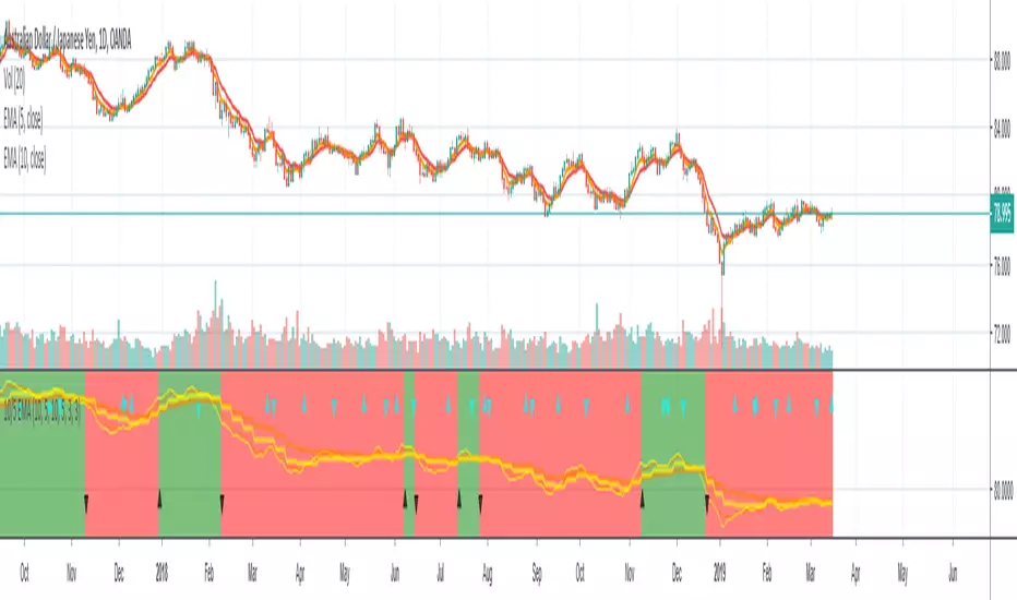
PRO Scalper(EN)
## What it is
**PRO Scalper** is an intraday price–action and liquidity map that helps you see where the market is likely to move **now**, not just where it has been.
It combines five building blocks that professional scalpers often watch together:
1. **Session Volume-Weighted Average Price (VWAP)** — the intraday “fair value” anchor.
2. **Opening Range** — the first minutes of the session that set the day’s balance.
3. **Trend filter** — higher-timeframe bias using **Exponential Moving Averages (EMA)** and optional **Average Directional Index (ADX)** strength.
4. **Two independent Supply/Demand zone engines** — zones are drawn from confirmed swing pivots, with midlines and **touch counters**.
5. **Order-flow style visuals**:
* **Delta bubbles** (green/red circles) show where buying or selling pressure was unusually strong, using a safe **delta proxy** (no external feeds).
* **Liquidity densities** (subtle rectangular bands) highlight clusters of large activity that often act as magnets or barriers and disappear when “eaten” by strong moves.
This mix gives you a **complete intraday picture**: the mean (VWAP), the day’s initial balance (Opening Range), the higher-timeframe push (trend filter), the nearby fuel or brakes (zones), and the live pressure points (bubbles and densities).
---
## Why these components
* **VWAP** tracks where the bulk of traded value sits. Price tends to rotate around it or accelerate away from it — a perfect compass for scalps.
* **Opening Range** frames the early auction. Many intraday breaks, fades and retests start at its boundaries.
* **EMA bias + ADX strength** separates trending conditions from chop, so you can keep only the zones that agree with the bigger push.
* **Pivot-based zones (two pairs at once)** are simple, objective and fast. Midlines help with confirmations; touch counters quantify how many times the zone was tested.
* **Bubbles and densities** add the “effort” layer: where the push appeared and where liquidity is concentrated. You see **where** a move is likely to continue or fail.
Together they reduce ambiguity: **context + level + effort** — all on one screen.
---
## How it works (plain language)
* **VWAP** resets each day and is calculated as the cumulative sum of typical price multiplied by volume divided by total volume.
* **Opening Range** is either automatic (a multiple of your chart timeframe) or a manual number of minutes. While it is forming, the highest high and lowest low are captured and plotted as the range.
* **Trend filter**
* **EMA Fast** and **EMA Slow** define directional bias.
* **ADX (optional)** adds “trend strength”: only when the Average Directional Index is above the chosen threshold do we treat the move as strong. You can source this from a higher timeframe.
* **Zones**
* There are **two independent pairs** of pivots at the same time (for example 10-left 10-right and 5-left 5-right).
* Each detected pivot creates a **Supply** (from a swing high) or **Demand** (from a swing low) box. Box depth = **zone depth × Average True Range** for adaptive sizing; the boxes **extend forward**.
* Midline (optional dashed line inside the box) is the “balance” of the zone.
* **“Only in trend”** mode can hide boxes that go against the higher-timeframe bias.
* The **touch counter** increases when price revisits the box. Labels show the pair name and the number of touches.
* **Bubbles**
* A safe **delta proxy** measures bar pressure (for example, range-weighted close vs open).
* A **quantile filter** shows only unusually large pressure: choose lookback and percentile, and the script draws a circle sized by intensity (green = bullish pressure, red = bearish).
* **Densities**
* The script marks heavy activity clusters as **subtle bands** around price (depth = fraction of Average True Range).
* If price **breaks** a density with volume above its moving average, the band **disappears** (“eaten”), which often precedes continuation.
---
## How to use — practical playbooks
> Recommended chart: crypto or index futures, one to five minutes. Use **one hour** or **fifteen minutes** for the higher-timeframe bias.
### 1) Trend pullback scalp (continuation)
1. Enable **Only in trend** zones.
2. In an uptrend: wait for a pullback into a **Demand** zone that overlaps with VWAP or sits just below the Opening Range midpoint.
3. Look for **green bubbles** near the zone’s bottom or a fresh **density** under price.
4. Enter on a candle closing **back above the zone midline**.
5. Stop-loss: below the bottom of the zone or a small multiple of Average True Range.
6. Targets: previous swing high, Opening Range high, fixed risk multiples, or VWAP.
Mirror the logic for downtrends using Supply zones, red bubbles and densities above price.
### 2) Reversion with liquidity sweep (fade)
1. Bias neutral or countertrend allowed.
2. Price **wicks through** a zone boundary (or an Opening Range line) and **closes back inside** the zone.
3. The bubble color often flips (absorption).
4. Enter toward the **inside** of the zone; stop beyond the sweep wick; first target = zone midline, second = opposite side of the zone or VWAP.
### 3) Opening Range break and retest
1. Wait for the Opening Range to complete.
2. A break with a large bubble suggests intent.
3. Look for a **retest** into a nearby zone aligned with VWAP.
4. Trade continuation toward the next zone or the session extremes.
### 4) Density “eaten” continuation
1. When a density band **disappears** on high volume, it often means the resting liquidity was consumed.
2. Trade in the direction of the break, toward the nearest opposing zone.
---
## Settings — quick guide
**Core**
* *ATR Length* — used for zone and density depths.
* *Show VWAP / Show Opening Range*.
* *Opening Range*: Auto (multiple of timeframe minutes) or Manual minutes.
**Trend Filter**
* *Mode*: Off, EMA only, or EMA with ADX strength.
* *Use higher timeframe* and its value.
* *EMA Fast / EMA Slow*, *ADX Length*, *ADX threshold*.
* *Plot EMA filter* to display the moving averages.
**Zones (two pairs)**
* *Pivot A Left / Right* and *Pivot B Left / Right*.
* *Zone depth × ATR*, *Extend bars*.
* *Show zone midline*, *Only in trend zones*.
* Labels automatically show the touch counters.
**Bubbles**
* *Show Bubbles*.
* *Quantile lookback* and *Quantile percent* (higher percent = stricter filter, fewer bubbles).
**Densities**
* *Metric*: absolute delta proxy or raw volume.
* *Quantile lookback / percent*.
* *Depth × ATR*, *Extend bars*, *Merge distance* (in ATR),
* *Break condition*: volume moving average length and multiplier,
* *Midline for densities* (optional dashed line).
---
## Tips and risk management
* This script **does not use external order-flow feeds**. Delta is a **proxy** suitable for TradingView; tune quantiles per symbol and timeframe.
* Do not trade every bubble. Combine **context (trend + VWAP + Opening Range)** with **level (zone)** and **effort (bubble/density)**.
* Set stop-losses beyond the zone or at a fraction of Average True Range. Predefine risk per trade.
* Backtest your rules with a strategy script before using real funds.
* Markets differ. Parameters that work on Bitcoin may not transfer to low-liquidity altcoins or stocks.
* Nothing here is financial advice. Scalping is high-risk; slippage and over-trading can quickly damage your account.
---
## What makes PRO Scalper unique
* Two **independent** zone engines run in parallel, so you can see both **larger structure** and **fine intraday levels** at the same time.
* Clean **“only in trend” rendering** — zones and midlines against the bias can be hidden, reducing clutter and hesitation.
* **Touch counters** convert “feel” into numbers.
* **Self-contained order-flow visuals** (bubbles and densities) that require no extra data sources.
* Careful defaults: subtle colors for densities, clearer zones, and responsive auto Opening Range.
---
(RU)
## Что это такое
**PRO Scalper** — это индикатор для внутридневной торговли, который показывает **контекст и ликвидность прямо сейчас**.
Он объединяет пять модулей, которыми профессиональные скальперы пользуются вместе:
1. **VWAP** — средневзвешенная по объему цена за сессию, «справедливая стоимость» дня.
2. **Opening Range** — первая часть сессии, задающая баланс дня.
3. **Фильтр тренда** — направление старшего таймфрейма по **экспоненциальным средним** и при желании по силе тренда **Average Directional Index**.
4. **Две независимые системы зон спроса/предложения** — зоны строятся от подтвержденных экстремумов (пивотов), имеют **среднюю линию** и **счетчик касаний**.
5. **Визуализация «ордер-флоу»**:
* **Пузыри дельты** (зеленые/красные круги) — места повышенного покупательного/продажного давления, рассчитанные через безопасный **прокси-дельты**.
* **Плотности ликвидности** (ненавязчивые прямоугольные ленты) — скопления объема, которые нередко притягивают цену или удерживают ее и исчезают, когда «разъедаются» сильным движением.
Итог — **полная картинка момента**: среднее (VWAP), баланс дня (Opening Range), старшая сила (фильтр тренда), ближайшие уровни топлива/тормозов (зоны), текущие точки усилия (пузыри и плотности).
---
## Почему именно эти элементы
* **VWAP** показывает, где сосредоточена стоимость; цена либо вращается вокруг него, либо быстро уходит — идеальный ориентир скальпера.
* **Opening Range** фиксирует ранний аукцион — от его границ часто начинаются пробои, возвраты и ретесты.
* **EMA + ADX** отделяют тренд от «пилы», позволяя оставлять на графике только зоны по направлению старшего таймфрейма.
* **Зоны от пивотов** просты, объективны и быстры; средняя линия помогает подтверждать разворот, счетчик касаний переводит субъективность в цифры.
* **Пузыри и плотности** добавляют слой «усилия»: где именно возник толчок и где сконцентрирована ликвидность.
Комбинация **контекста + уровня + усилия** уменьшает двусмысленность и ускоряет принятие решения.
---
## Как это работает (простыми словами)
* **VWAP** каждый день стартует заново: сумма «типичной цены × объем» делится на суммарный объем.
* **Opening Range** — автоматический (кратный минутам вашего таймфрейма) или вручную заданный период; пока он формируется, фиксируются максимум и минимум.
* **Фильтр тренда**
* Две экспоненциальные средние задают направление.
* **ADX** (по желанию) добавляет «силу». Источник можно взять со старшего таймфрейма.
* **Зоны**
* Одновременно работает **две пары** пивотов (например 10-лево 10-право и 5-лево 5-право).
* От пивота строится зона **предложения** (от максимума) или **спроса** (от минимума). Глубина зоны = **коэффициент × Average True Range**; зона тянется вперед.
* Внутри рисуется **средняя линия** (по желанию).
* Режим **«только по тренду»** скрывает зоны против старшего направления.
* **Счетчик касаний** увеличивается, когда цена снова входит в зону; подпись показывает пару и количество касаний.
* **Пузыри**
* Используется безопасный **прокси-дельты** — измерение «напряжения» внутри свечи.
* Через **квантильный фильтр** выводятся только необычно сильные места: настраиваются окно и процент квантиля; размер кружка — сила, цвет: зеленый покупатели, красный продавцы.
* **Плотности**
* Крупные активности отмечаются **ненавязчивыми прямоугольниками** (глубина — доля Average True Range).
* Если плотность **пробивается** объемом выше среднего, она **исчезает** — часто это предвещает продолжение.
---
## Как пользоваться — практические схемы
> Рекомендация: крипто или фьючерсы, таймфрейм 1–5 минут. Для старшего фильтра удобно взять **1 час** или **15 минут**.
### 1) Скальп на откат по тренду
1. Включите **«только по тренду»**.
2. В восходящем тренде дождитесь отката в **зону спроса**, желательно рядом с **VWAP** или серединой **Opening Range**.
3. Подтверждение — **зеленые пузыри** у нижней границы зоны или свежая **плотность** под ценой.
4. Вход после закрытия свечи **выше средней линии** зоны.
5. Стоп-лосс: за нижнюю границу зоны или небольшой множитель Average True Range.
6. Цели: предыдущий максимум, верх Opening Range, фиксированные R-множители, либо VWAP.
Для нисходящего тренда зеркально: зоны предложения, красные пузыри и плотности над ценой.
### 2) Контрдвижение с «выбиванием ликвидности»
1. Нейтральный или контртрендовый режим.
2. Цена **выносит хвостом** границу зоны (или линию Opening Range) и **закрывается обратно внутри**.
3. Цвет пузыря часто меняется (поглощение).
4. Вход внутрь зоны; стоп — за хвост выбивания; цели: средняя линия, противоположная граница зоны или VWAP.
### 3) Пробой Opening Range + ретест
1. Дождитесь завершения диапазона.
2. Сильный пробой с крупным пузырем — признак намерения.
3. Ищите **ретест** в зоне по тренду рядом с линией диапазона и VWAP.
4. Торгуйте продолжение к следующей зоне.
### 4) Продолжение после «съеденной» плотности
1. Когда прямоугольник плотности **исчезает** на повышенном объеме, это значит, что ликвидность поглощена.
2. Торгуйте в сторону пробоя к ближайшей противоположной зоне.
---
## Настройки — краткая шпаргалка
**Core**
— Длина Average True Range (для размеров зон и плотностей).
— Включение VWAP и Opening Range.
— Длина Opening Range: автоматическая (кратная минутам ТФ) или ручная.
**Trend Filter**
— Режим: выкл., только средние, либо средние + ADX.
— Источник со старшего таймфрейма и его значение.
— Длины средних, длина ADX и порог силы.
— Показать/скрыть линий средних.
**Zones (две пары одновременно)**
— Пара A: лев/прав; Пара B: лев/прав.
— Глубина зоны × Average True Range, продление по барам.
— Средняя линия, режим **«только по тренду»**.
— Подписи со счетчиком касаний.
**Bubbles**
— Вкл./выкл., окно поиска и процент квантиля (чем выше процент — тем реже пузыри).
**Densities**
— Метрика: абсолютная прокси-дельты или чистый объем.
— Окно/квантиль, глубина × Average True Range, продление,
— Порог объединения (в Average True Range),
— Условие «разъедания» по объему,
— Средняя линия плотности (по желанию).
---
## Советы и риски
* Индикатор **не использует внешние потоки ордер-флоу**. Дельта — **прокси**, подходящая для TradingView; подбирайте квантили под инструмент и таймфрейм.
* Не торгуйте каждый пузырь. Склейте **контекст (тренд + VWAP + Opening Range)** с **уровнем (зона)** и **усилием (пузырь/плотность)**.
* Стоп-лосс — за границей зоны или по Average True Range. Риск на сделку задавайте заранее.
* Перед реальными деньгами протестируйте правила в стратегии.
* Разные рынки ведут себя по-разному; настройки из Биткоина могут не подойти малоликвидным альткоинам или акциям.
* Это не инвестиционная рекомендация. Скальпинг — высокий риск; проскальзывание и переизбыток сделок быстро наносят ущерб капиталу.
---
## Чем уникален PRO Scalper
* Две **одновременные** системы зон показывают и **крупную структуру**, и **точные локальные уровни**.
* Режим **«только по тренду»** чистит экран от лишних уровней и ускоряет решение.
* **Счетчики касаний** дают количественную опору.
* **Самодостаточные визуализации усилия** (пузыри и плотности) — без сторонних источников данных.
* Аккуратная цветовая схема: плотности — мягко, зоны — ясно; Opening Range — адаптивный.
Пусть он станет вашей «картой местности» для быстрых и дисциплинированных решений внутри дня.
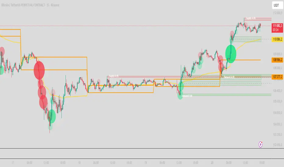
Uptrick: Volatility Weighted CloudIntroduction
The Volatility Weighted Cloud (VWC) is a trend-tracking overlay that combines adaptive volatility-based bands with a multi-source smoothed price cloud to visualize market bias. It provides users with a dynamic structure that adapts to volatility conditions while maintaining a persistent visual record of trend direction. By incorporating configurable smoothing techniques, percentile-ranked volatility, and multi-line cloud construction, the indicator allows traders to interpret price context more effectively without relying on raw price movement alone.
Overview
The script builds a smoothed price basis using the open, and close prices independently, and uses these to construct a layered visual cloud. This cloud serves both as a reference for price structure and a potential area of dynamic support and resistance. Alongside this cloud, adaptive upper and lower bands are plotted using volatility that scales with percentile rank. When price closes above or below these bands, the script interprets that as a breakout and updates the trend bias accordingly.
Candle coloring is persistent and reflects the most recent confirmed signal. Labels can optionally be placed on the chart when the trend bias flips, giving traders additional visual reference points. The indicator is designed to be both flexible and visually compact, supporting different strategies and timeframes through its detailed configuration options.
Originality
This script introduces originality through its combined use of percentile-ranked volatility, adaptive envelope sizing, and multi-source cloud construction. Unlike static-band indicators, the Volatility Weighted Cloud adjusts its band width based on where current volatility ranks within a defined lookback range. This dynamic scaling allows for smoother signal behavior during low-volatility environments and more responsive behavior during high-volatility phases.
Additionally, instead of using a single basis line, the indicator computes two separate smoothed lines for open and close. These are rendered into a shaded visual cloud that reflects price structure more completely than traditional moving average overlays. The use of ALMA and MAD, both less commonly applied in volatility-band overlays, adds further control over smoothing behavior and volatility measurement, enhancing its adaptability across different market types.
Inputs
Group: Core
Basis Length (short-term): The number of bars used for calculating the primary basis line. Affects how quickly the basis responds to price changes.
Basis Type: Option to choose between EMA and ALMA. EMA provides a standard exponential average; ALMA offers a centered, Gaussian-weighted average with reduced lag.
ALMA Offset: Determines the balance point of the ALMA window. Only applies when ALMA is selected.
Sigma: Sets the width of the ALMA smoothing window, influencing how much smoothing is applied.
Basis Smoothing EMA: Adds additional EMA-based smoothing to the computed basis line for noise reduction.
Group: Volatility & Bands
Volatility: Choose between StDev (standard deviation) and MAD (median absolute deviation) for measuring price volatility.
Vol Length (short-term): Length of the window used for calculating volatility.
Vol Smoothing EMA: Smooths the raw volatility value to stabilize band behavior.
Min Multiplier: Minimum multiplier applied to volatility when forming the adaptive bands.
Max Multiplier: Maximum multiplier applied at high volatility percentile.
Volatility Rank Lookback: Number of bars used to calculate the percentile rank of current volatility.
Show Adaptive Bands: Enables or disables the display of upper and lower volatility bands on the chart.
Group: Trend Switch Labels
Show Trend Switch Labels: Toggles the appearance of labels when the trend direction changes.
Label Anchor: Defines whether the labels are anchored to recent highs/lows or to the main basis line.
ATR Length (offset): Length used for calculating ATR, which determines label offset distance.
ATR Offset (multiplier): Multiplies the ATR value to place labels away from price bars for better visibility.
Label Size: Allows selection of label size (tiny to huge) to suit different chart setups.
Features
Adaptive Volatility Bands: The indicator calculates volatility using either standard deviation or MAD. It then applies an EMA smoothing layer and scales the band width dynamically based on the percentile rank of volatility over a user-defined lookback window. This avoids fixed-width bands and allows the indicator to adapt to changing volatility regimes in real time.
Volatility Method Options: Users can switch between two volatility measurement methods:
➤ Standard Deviation (StDev): Captures overall price dispersion, but may be sensitive to spikes.
➤ Median Absolute Deviation (MAD): A more robust measure that reduces the effect of outliers, making the bands less jumpy during erratic price behavior.
Basis Type Options: The core price basis used for cloud and bands can be built from:
➤ Exponential Moving Average (EMA): Fast-reacting and widely used in trend systems.
➤ Arnaud Legoux Moving Average (ALMA): A smoother, more centered alternative that offers greater control through offset and sigma parameters.
Multi-Line Basis Cloud: The cloud is formed by plotting two individually smoothed basis lines from open and close prices. A filled area is created between the open and close basis lines. This cloud serves as a dynamic support or resistance zone, allowing users to identify possible reversal areas. Price moving through or rejecting from the cloud can be interpreted contextually, especially when combined with band-based signals.
Persistent Trend Bias Coloring: The indicator uses the last confirmed breakout (above upper band or below lower band) to determine bias. This bias is reflected in the color of every subsequent candle, offering a persistent visual cue until a new signal is triggered. It helps simplify trend recognition, especially in choppy or sideways markets.
Trend Switch Labels: When enabled, the script places labeled markers at the exact bar where the bias direction switches. Labels are anchored either to recent highs/lows or to the main basis line, and spaced vertically using an ATR-based offset. This allows the trader to quickly locate historical trend transitions.
Alert Conditions: Two built-in alert conditions are available:
➤ Long Signal: Triggered when the close crosses above the upper adaptive band.
➤ Short Signal: Triggered when the close crosses below the lower adaptive band.
These conditions can be used for custom alerts, automation, or external signaling tools.
Display Control and Flexibility: Users can disable the adaptive bands for a cleaner layout while keeping the basis cloud and candle coloring active. The indicator can be tuned for fast or slow response depending on the strategy in use, and is suitable for intraday, swing, or position trading.
Summary
The Volatility Weighted Cloud is a configurable trend-following overlay that uses adaptive volatility bands and a structured cloud system to help visualize market bias. By combining EMA or ALMA smoothing with percentile-ranked volatility and a four-line price structure, it provides a flexible and informative charting layer. Its key strengths lie in the use of dynamic envelopes, visually persistent trend indication, and clearly defined breakout zones that adapt to current volatility conditions.
Disclaimer
This indicator is for informational and educational purposes only. Trading involves risk and may not be suitable for all investors. Past performance does not guarantee future results.

ATR Trailing Stop with ATR Targets [v6]What the Indicator Does
This custom TradingView indicator is designed for active traders who want to automate and visualize their trailing stop management and target setting, using true market volatility. It combines the Average True Range (ATR) with dynamic market structure logic to:
Trail a stop-loss behind major swings in real time, using 2×ATR (adjustable) from the highest high in uptrends or the lowest low in downtrends.
Flip trading bias between bullish and bearish when the stop is breached.
Identify and plot three profit targets (at 1, 2, and 3 ATR from the breakout/flip point) after every stop-flip, helping traders scale out or set take-profits objectively.
Maintain a visible presence on your chart every bar to avoid indicator errors, with color and labeling for clear distinction between long/short phases.
How the Indicator Works
1. ATR Calculation
ATR Period and Multiplier: You select your preferred ATR length (default is 14 bars) and a multiplier (default is 2.0).
Volatility Adjustment: ATR measures the average "true" bar range, so the trailing stop and targets adapt to current volatility.
2. Trailing Stop Logic
Uptrend (bullish bias): The indicator tracks the highest high made since the last bearish-to-bullish flip and sets the stop at - .
The stop only raises (never lowers) during an uptrend, protecting gains in strong moves.
Downtrend (bearish bias): Tracks the lowest low made since the last bullish-to-bearish flip, with stop at + .
The stop only lowers (never raises) in a downtrend.
Flip Point: If price closes through the trailing stop, the current bias “flips,” and the logic reverses (bullish to bearish or vice versa). At the new close, flip price and bar index are stored for target calculation.
3. ATR Targets after Flip
After each stop flip:
Three targets—based on the new close price—are calculated and plotted:
Long flip (new bull bias): Target1 = close + 1×ATR, Target2 = close + 2×ATR, Target3 = close + 3×ATR.
Short flip (new bear bias): Target1 = close - 1×ATR, Target2 = close - 2×ATR, Target3 = close - 3×ATR.
These targets help with scaling out, partial profit-taking, or setting automated orders.
4. Visual Feedback
Trailing stop line: Green for long bias, red for short bias.
Targets: Distinct color-coded circles at 1, 2, 3 ATR levels from the most recent flip.
Flip Labels: Mark the bar and price where bias flipped (“Long Flip” or “Short Flip”) for quick pattern recognition.
Subtle background shading: Ensures TradingView's requirement for “indicator output every bar.”
How to Use This Indicator
Parameter Setup
ATR Period and Multiplier: Adjust to match the timeframe and volatility of your instrument.
Lower periods/multipliers for short-term/volatile trading.
Higher values for smoother signals or higher timeframes.
Starting Trend: Set to match the expected initial bias if the instrument has strong trend characteristics.
Trading Application
1. Daily Bias Approach
Establish your bias in line with your trading plan (e.g., only trade long if price is above the previous day's high, short below the previous day's low).
Only look for trades in the indicator's current bias direction, as expressed by the stop and background color.
2. Entry
Use the indicator as a real-time confirmation or trailing stop for your entries.
Breakout: Enter when price establishes the current bias, using the trailing stop as your risk level.
Reversal: Wait for a bias flip after an extended move; enter in the direction of the new bias.
VWAP Rebound: Combine with a VWAP bounce—enter only if the indicator bias supports your direction.
3. Exits/Targets
Trailing stop management: Move your stop according to the plotted line; exit if your stop is hit.
Profit-taking: Scale out or take profits as price approaches each ATR-based target.
Use the dynamic labeling to identify reversal flips and reset your plan if stopped or the bias changes.
4. Market Context
Filter and frame setups by watching correlated indicators (DXY, VIX, AUDJPY, put/call ratio) and upcoming news; trade only in the daily bias direction for best consistency.
5. Practical Tips
Combine this indicator with your custom watchlist and alert settings to get notified on flips or targets.
Review the last label ("Long Flip"/"Short Flip") and targets to plan partial exits.
Remember: ATR adapts to volatility, so the stop and targets stay proportionate even when price action shifts.
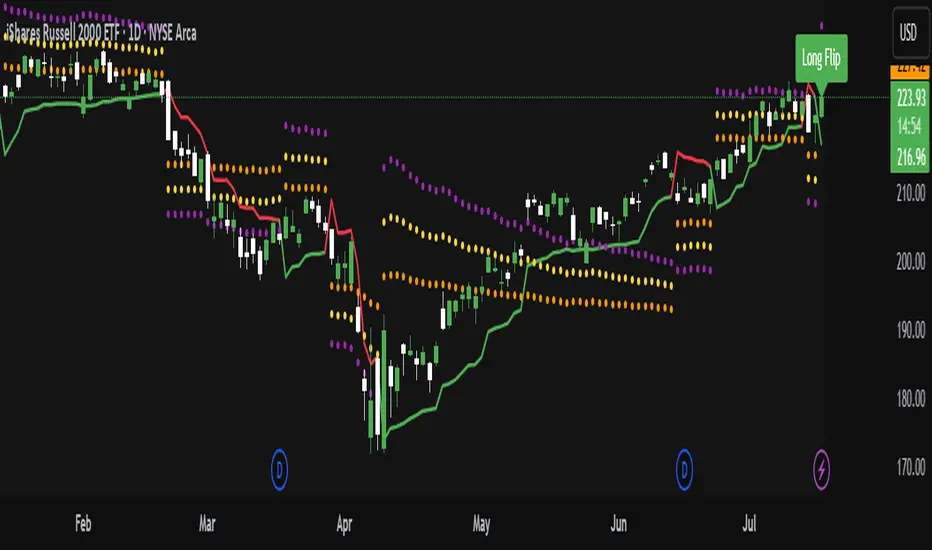
Linear Regression Forecast (ADX Adaptive)Linear Regression Forecast (ADX Adaptive)
This indicator is a dynamic price projection tool that combines multiple linear regression forecasts into a single, adaptive forecast curve. By integrating trend strength via the ADX and directional bias, it aims to visualize how price might evolve in different market environments—from strong trends to mean-reverting conditions.
Core Concept:
This tool builds forward price projections based on a blend of linear regression models with varying lookback lengths (from 2 up to a user-defined max). It then adjusts those projections using two key mechanisms:
ADX-Weighted Forecast Blending
In trending conditions (high ADX), the model follows the raw forecast direction. In ranging markets (low ADX), the forecast flips or reverts, biasing toward mean-reversion. A logistic transformation of directional bias, controlled by a steepness parameter, determines how aggressively this blending reacts to price behavior.
Volatility Scaling
The forecast’s magnitude is scaled based on ADX and directional conviction. When trends are unclear (low ADX or neutral bias), the projection range expands to reflect greater uncertainty and volatility.
How It Works:
Regression Curve Generation
For each regression length from 2 to maxLength, a forward projection is calculated using least-squares linear regression on the selected price source. These forecasts are extrapolated into the future.
Directional Bias Calculation
The forecasted points are analyzed to determine a normalized bias value in the range -1 to +1, where +1 means strongly bullish, -1 means strongly bearish, and 0 means neutral.
Logistic Bias Transformation
The raw bias is passed through a logistic sigmoid function, with a user-defined steepness. This creates a probability-like weight that favors either following or reversing the forecast depending on market context.
ADX-Based Weighting
ADX determines the weighting between trend-following and mean-reversion modes. Below ADX 20, the model favors mean-reversion. Above 25, it favors trend-following. Between 20 and 25, it linearly blends the two.
Blended Forecast Curve
Each forecast point is blended between trend-following and mean-reverting values, scaled for volatility.
What You See:
Forecast Lines: Projected future price paths drawn in green or red depending on direction.
Bias Plot: A separate plot showing post-blend directional bias as a percentage, where +100 is strongly bullish and -100 is strongly bearish.
Neutral Line: A dashed horizontal line at 0 percent bias to indicate neutrality.
User Inputs:
-Max Regression Length
-Price Source
-Line Width
-Bias Steepness
-ADX Length and Smoothing
Use Cases:
Visualize expected price direction under different trend conditions
Adjust trading behavior depending on trending vs ranging markets
Combine with other tools for deeper analysis
Important Notes:
This indicator is for visualization and analysis only. It does not provide buy or sell signals and should not be used in isolation. It makes assumptions based on historical price action and should be interpreted with market context.
Weighted Momentum Forecast
The Weighted Momentum Forecast (EWMF) is a predictive indicator designed to forecast the potential direction and magnitude of the next candle's close. It combines the principles of momentum, trend confirmation, and volatility adjustment to make its predictions.
**Components:**
1. **Rate of Change (ROC)**: Measures the momentum of the market.
2. **Average True Range (ATR)**: Represents the market's recent volatility.
3. **Moving Average Convergence Divergence (MACD)**: Used to confirm the momentum's direction.
4. **Trend Moving Average**: A longer-term moving average to confirm the general trend.
5. **Bollinger Bands**: Adjusts the forecast to account for extreme predictions.
**Logic:**
1. **Momentum Bias**: The crossover and crossunder of the MACD line and its signal line are used to determine the momentum's bias. A crossover indicates a bullish bias, while a crossunder indicates a bearish bias.
2. **Trend Confirmation**: If the current close is above the trend moving average, the indicator has a bullish bias, and vice versa.
3. **Forecast Calculation**: The forecast for the next candle's close is calculated based on the current close, the rate of change, the momentum's bias, and the trend's bias. This value is then adjusted for volatility using the ATR.
4. **Volatility Adjustment**: If the forecasted value is beyond the Bollinger Bands, it's adjusted to be within the bands to account for extreme predictions.
**Usage:**
The EWMF plots a purple line representing the forecasted value of the next candle's close. This forecasted value provides traders with a visual representation of where the price might head in the next period, based on recent momentum, trend, and volatility.
**Note**: This is a heuristic approach and is not guaranteed to be accurate. It's essential to use this indicator in conjunction with other tools, backtest on historical data, and use proper risk management techniques. Always be aware of the inherent risks involved in trading and never risk more than you're willing to lose.
DDDDD : EMA Pack (Matched Colors + MTF)📌 DDDDD : EMA Pack (Matched Colors + MTF)
🔹 Concept
DDDDD : EMA Pack is a clean and minimal Exponential Moving Average (EMA) overlay designed for trend structure analysis and multi-timeframe context.
This indicator focuses on visual clarity, consistent color mapping, and optional MTF EMA projection, allowing traders to read market structure without clutter or signal noise.
It is not an entry or signal generator, but a trend and regime visualization tool.
🔹 Logic
The script plots a fixed set of EMAs commonly used to define short-term momentum, intermediate trend, and long-term bias:
EMA 5
EMA 10
EMA 25
EMA 50
EMA 75
EMA 200
Each EMA is calculated using the standard exponential moving average formula.
If a higher timeframe is selected, the EMA is calculated on that timeframe and projected onto the current chart using request.security().
🔹 Methodology
Users may select:
Source price (default: close)
EMA timeframe
Empty = current chart timeframe
Any higher timeframe = true MTF EMA projection
All EMA colors are manually matched and fixed to maintain visual consistency across markets and timeframes.
Line thickness is kept uniform to avoid visual hierarchy bias.
This design ensures the indicator remains purely structural, without repainting logic, smoothing tricks, or adaptive parameters.
🔹 How to Use
Use EMA alignment and spacing to assess:
Trend direction
Trend strength
Compression vs expansion
Higher-timeframe EMA projection can be used as:
Dynamic support/resistance
Trend filter
Regime context for lower-timeframe execution
This indicator works best when combined with:
Price action
Market structure
Separate entry/exit logic of your own system
⚠️ This indicator does not provide buy/sell signals and should not be used alone for trade execution.
🔹 Notes
No repainting beyond standard MTF behavior
No performance or profitability claims
Designed for discretionary and systematic traders
Suitable for stocks, crypto, forex, and indices

Execution Heatmap v4.1 — AI EnhancedThis indicator is an AI‑style execution dashboard that compresses structure, momentum, volume, volatility, and risk into a compact heatmap panel plus BUY/SELL signals on the chart. It is specifically tuned for gold and silver, automatically adapting its thresholds to the volatility profile of XAU/GC and XAG/SI symbols.
Core architecture
The system builds a multi‑factor model in layers:
Adaptive structure engine: Tracks dynamic higher‑high / lower‑low progression using rolling reference highs and lows, classifying price as structural UP, DOWN, or NEUTRAL.
Precision VWAP bias: Uses VWAP with a small threshold band to filter out noise and label price as ABOVE, BELOW, or neutral relative to value.
Impulse & angle: Combines short‑term rate of change and normalized slope (price vs ATR over 5 bars) to detect directional thrust, then clamps values into
for stable scoring.
Volume, wicks, and patterns
Adaptive volume tiers: Uses a 20‑bar volume average with gold/silver‑specific multipliers to tag candles as SURGE, HIGH, NORMAL, or LOW volume, with distinct coloring for extremes.
Wick analytics: Measures upper/lower wick size vs total range to detect demand/supply style rejections and encode them as bullish or bearish wick signals.
AI pattern score: Blends structure, VWAP, impulse, wicks, and angle into a normalized pattern score, then classifies it as STRONG↑, NEU↑, NEU, NEU↓, or STRONG↓ with color‑coded emphasis.
AI scoring and prediction layer
Predictive engine: Uses a neural‑network‑style weighted sum of structure, VWAP, impulse, wicks, angle, volume, and pattern to generate a prediction score in
, then converts it into a percentage and arrow (↑, ↑↑, ↓, ↓↓, →) for intuitive directional bias.
Execution score: Aggregates key factors into an EXEC score (0–200+ style scale), color‑graded from weak (red) through medium (orange) to strong (green) execution context.
Uncertainty & risk: Separately models uncertainty (low impulse/angle or low conviction) and risk (fake breaks, VWAP position, uncertainty tier, low volume), then feeds them into a combined confidence calculation.
Final signal & confidence
Final classification:
BUY: High exec score, high confidence, and controlled risk.
SELL: Very low exec score, low confidence in upside, and acceptable risk.
WAIT: All other conditions where edge or clarity is insufficient.
Confidence bar: A textual mini‑bar (🟩 blocks) plus percentage shows how strong the current signal environment is, making it easy to visually gauge setup quality at a glance.
Professional heatmap panel
A two‑column table in the top‑right of the chart organizes the logic into layers:
Base layer: STRUCT, VWAP, IMPULSE, VOLUME.
AI layer: FAKE, REGIME (Trend/Pullback/Reverse/Chop), ANGLE.
Decision layer: PATTERN, PREDICT, EXEC, RISK, CONF, and FINAL direction.
Volatility Signal-to-Noise Ratio🙏🏻 this is VSNR: the most effective and simple volatility regime detector & automatic volatility threshold scaler that somehow no1 ever talks about.
This is simply an inverse of the coefficient of variation of absolute returns, but properly constructed taking into account temporal information, and made online via recursive math with algocomplexity O(1) both in expanding and moving windows modes.
How do the available alternatives differ (while some’re just worse)?
Mainstream quant stat tests like Durbin-Watson, Dickey-Fuller etc: default implementations are ALL not time aware. They measure different kinds of regime, which is less (if at all) relevant for actual trading context. Mix of different math, high algocomplexity.
The closest one is MMI by financialhacker, but his approach is also not time aware, and has a higher algocomplexity anyways. Best alternative to mine, but pls modify it to use a time-weighted median.
Fractal dimension & its derivatives by John Ehlers: again not time aware, very low info gain, relies on bar sizes (high and lows), which don’t always exist unlike changes between datapoints. But it’s a geometric tool in essence, so this is fundamental. Let it watch your back if you already use it.
Hurst exponent: much higher algocomplexity, mix of parametric and non-parametric math inside. An invention, not a math entity. Again, not time aware. Also measures different kinds of regime.
How to set it up:
Given my other tools, I choose length so that it will match the amount of data that your trading method or study uses multiplied by ~ 4-5. E.g if you use some kind of bands to trade volatility and you calculate them over moving window 64, put VSNR on 256.
However it depends mathematically on many things, so for your methods you may instead need multipliers of 1 or ~ 16.
Additionally if you wanna use all data to estimate SNR, put 0 into length input.
How to use for regime detection:
First we define:
MR bias: mean reversion bias meaning volatility shorts would work better, fading levels would work better
Momo bias: momentum bias meaning volatility longs would work better, trading breakouts of levels would work better.
The study plots 3 horizontal thresholds for VSNR, just check its location:
Above upper level: significant Momo bias
Above 1 : Momo bias
Below 1 : MR bias
Below lower level: significant MR bias
Take a look at the screenshots, 2 completely different volatility regimes are spotted by VSNR, while an ADF does not show different regime:
^^ CBOT:ZN1!
^^ INDEX:BTCUSD
How to use as automatic volatility threshold scaler
Copy the code from the script, and use VSNR as a multiplier for your volatility threshold.
E.g you use a regression channel and fade/push upper and lower thresholds which are RMSEs multiples. Inside the code, multiply RMSE by VSNR, now you’re adaptive.
^^ The same logic as when MM bots widen spreads with vola goes wild.
How it works:
Returns follow Laplace distro -> logically abs returns follow exponential distro , cuz laplace = double exponential.
Exponential distro has a natural coefficient of variation = 1 -> signal to noise ratio defined as mean/stdev = 1 as well. The same can be said for Student t distro with parameter v = 4. So 1 is our main threshold.
We can add additional thresholds by discovering SNRs of Student t with v = 3 and v = 5 (+- 1 from baseline v = 4). These have lighter & heavier tails each favoring mean reversion or momentum more. I computed the SNR values you see in the code with mpmath python module, with precision 256 decimals, so you can trust it I put it on my momma.
Then I use exponential smoothing with properly defined alphas (one matches cumulative WMA and another minimizes error with WMA in moving window mode) to estimate SNR of abs returns.
…
Lightweight huh?
∞