72s Strat: Backtesting Adaptive HMA+ pt.1This is a follow up to my previous publication of Adaptive HMA+ few months ago, as a mean to provide some kind of initial backtesting tools. Which can be use to explore many possible strategies, optimise its settings to better conform user's pair/tf, and hopefully able to help tweaking your general strategy.
If you haven't read the study or use the indicator, kindly go here first to get the overall idea.
The first strategy introduce in this backtest is one most basic already described in the study; buy/sell is when movement is there and everything is on the right side; When RSI has turned to other side, we can use it as exit point (if in profit of course, else just let it hit our TP/SL, why would we exit before profit). Also, base on RSI when we make entry, we can further differentiate type of signals. --Please check all comments in code directly where the signals , entries , and exits section are.
Second additional strategy to check; is when we also use second faster Adaptive HMA+ for exit. So this is like a double orders on a signal but with different exit-rule (/more on this on snapshots below). Alternatively, you can also work the code so to only use this type of exit.
There's also an additional feature which you can enable its visuals, the Distance Zone , is to help measuring price distance to our xHMA+. It's just a simple atr based envelope really, I already put the sample code in study's comment section, but better gonna update it there directly for non-coder too, after this.
In this sample I use Lot for order quantity size just because that's what I use on my broker. Also what few friends use while we forward-testing it since the study is published, so we also checked/compared each profit/loss report by real number. To use default or other unit of measurement, change the entry code accordingly.
If you change your order size, you should also change the commission in Properties Tab. My broker commission is 5 USD per order/lot, so in there with example order size 0.1 lot I put commission 0.5$ per order (I'll put 2.5$ for 0.5 lot, 10$ for 2 lot, and so on). Crypto usually has higher charge. --It is important that you should fill it base on your broker.
SETTINGS
I'm trying to keep it short. Please explore it further again. (Beginner should also first get acquaintance with terms use here.)
ORDERS:
Base Minimum Profit Before Exit:
The number is multiplier of ongoing ATR. Means that when basic exit condition is met, algo will check whether you're already in minimum profit or not, if not, let it still run to TP or SL, or until it meets subsequent exit condition, then it will check again.
Default Target Profit:
Multiplier of ATR at signal. If reached before any eligible exit condition is met, exit TP.
Base StopLoss Point:
You can change directly in code to use other like ATR Trailing SL, fix percent SL, or whatever. In the sample, 4 options provided.
Maximum StopLoss:
This is like a safety-net, that if at some point your chosen SL point from input above happens to be exceeding this maximum input that you can tolerate, then this max point is the one will be use as SL.
Activate 2nd order...:
The additional doubling of certain buy/sell with different exits as described above. If enable, you should also set pyramiding to at least: 2. If not, it does nothing.
ADAPTIVE HMA+ PERIOD
Many users already have their own settings for these. So in here I only sample the default as first presented in the study. Make it to your adaptive.
MARKET MOVEMENT
(1) Now you can check in realtime how much slope degree is best to define your specific pair/tf is out of congestion (yellow) area. And (2) also able to check directly what ATR lengths are more suitable defining your pair's volatility.
DISTANCE ZONE
Distance Multiplier. Each pair/tf has its own best distance zone (in xHMA+ perspective). The zone also determine whether a signal should appear or not. (Or what type of signal, if you wanna go more detail in constructing your strategy)
USAGE
(Provided you already have your own comfortable settings for minimum-maximum period of Adaptive HMA+. Best if you already have backtested it manually too and/or apply as an add-on to your working strategy)
1. In our experiences, first most important to define is both elements in the Market Movement Settings . These also tend to be persistent for whole season since it's kinda describing that pair/tf overall behaviour. Don't worry if you still get a low Profit Factor here, but by tweaking you should start to see positive changes in one of Max Drawdown and Net Profit, or Percent Profitable.
2. Afterwards, find your pair/tf Distance Zone . When optimising this, what we seek is just a "not to bad" equity curves to start forming. At least Max Drawdown should lessen more. Doesn't have to be great already, but should be better, no red in Net Profit.
3. Then go manage the "Trailing Minimum Profit", TP, SL, and max SL.
4. Repeat 1,2,3. 👻
5. Manage order size, commission, and/or enable double-order (need pyramiding) if you like. Check if your equity can handle max drawdown before margin call.
6. After getting an acceptable backtest result, go to List of Trades tab and find the biggest loss or when many sequencing loss in a row happened. Click on it to go to exact point on chart, observe why the signal failed and get at least general idea how it can be prevented . The rest is yours, you should know your pair/tf more than other.
You can also re-explore your minimum-maximum period for both Major and minor xHMA+.
Keep in mind that all numbers in Setting are conceptually in a form of range . You don't want to get superb equity curves but actually a "fragile" , means one can easily turn it to disaster just by changing only a fraction in one/two of the setting.
---
If you just wanna test the strength of the indicator alone, you can disable "Use StopLoss" temporarily while optimising settings.
Using no SL might be tempting in overall result data in some cases, but NOTE: It is not recommended to not using SL, don't forget that we deliberately enter when it's in high volatility. If want to add flexibility or trading for long-term, just maximise your SL. ie.: chose SL Point>ATR only and set it maximum. (Check your max drawdown after this).
I think this is quite important specially for beginners, so here's an example; Hypothetically in below scenario, because of some settings, the buy order after the loss sell signal didn't appear. Let's say if our initial capital only 1000$ using leverage and order size 0,5 lot (risky position sizing already), moreover if this happens at the beginning of your trading season, that's half of account gone already in one trade . Your max SL should've made you exit after that pumping bar.
The Trailing Minimum Profit is actually look like this. Search in the code if you want to plot it. I just don't like too many lines on chart.
To maximise profit we can try enabling double-order. The only added rule coded is: RSI should rising when buy and falling when sell. 2nd signal will appears above or below default buy/sell signal. (Of course it's also prone to double-loss, re-check your max drawdown after. Profit factor play its part in here for a long run). Snapshot in comparison:
Two default sell signals on left closed at RSI exit, the additional sell signal closed later on when price crossover minor xHMA+. On buy side, price haven't met our minimum profit when first crossunder minor xHMA+. If later on we hit SL on this "+buy" signal, at least we already profited from default buy signal. You can also consider/treat this as multiple TP points.
For longer-term trading, what you need to maximise is the Minimum Profit , so it won't exit whenever an exit condition happened, it can happen several times before reaching minimum profit. Hopefully this snapshot can explain:
Notice in comparison default sell and buy signal now close in average after 3 days. What's best is when we also have confirmation from higher TF. It's like targeting higher TF by entering from smaller TF.
As also mention in the study, we can still experiment via original HMA by putting same value for minimum-maximum period setting. This is experimental EU 1H with Major xHMA+: 144-144, Flat market 13, Distance multiplier 3.6, with 2nd order activated.
Kiwi was a bit surprising for me. It's flat market is effectively below 6, with quite far distance zone of 3.5. Probably because I'm using big numbers in adaptive period.
---
The result you see in strategy tester report below for EURUSD 15m is using just default settings you see in code, as follow:
0,1 lot for each order (which is the smallest allowed by my broker).
No pyramiding. Commission: 0.5 usd per order. Slippage: 3
Opening position is only using basic strategy #1 (RSI exit). Additional exit not activated.
Minimum Profit: 1. TP: 3.
SL use: Half-distance zone. Max SL: 4.5.
Major xHMA+: 172-233. minor xHMA+: 89-121
Distance Zone Multiplier: 2.7
RSI: Standard 14.
(From our forward-testing, the difference we get from net profit is because of the spread, our entry isn't exactly at the close/open price. Not so much though, but not the same. If somebody can direct me to any example where we can code our entry via current bid/ask price, that would be awesome!)
It's already a long post (sorry), think I'm gonna pause here. Check out the code :)
---
DISCLAIMER: Past performance is no guarantee of future results , and so on.. you know the drill ;)
Please read whole description first before using, don't take 1-2 paragraph and claim it's the whole logic, you are responsible of your own actions and understanding.
Search in scripts for "one一季度财报"

+ BB %B: MA selection, bar coloring, multi-timeframe, and alerts+ %B is, at its simplest, the classic Bollinger Bands %B indicator with a few added bells and whistles.
However, the right combination of bells and whistles will often improve and make a more adaptable indicator.
Classically, Bollinger Bands %B is an indicator that measures volatility, and the momentum and strength of a trend, and/or price movements.
It shows "overbought" and "oversold" spots on a chart, and is also useful for identifying divergences between price and trend (similar to RSI).
With + %B I've added the options to select one or two moving averages, candle coloring, and a host of others.
Let's start with the moving averages:
There are options for two: one faster and one slower. Or combine them how you will, or omit one or both of them entirely.
Here you will find options for SMA, EMA (as well as double and triple), Hull MA, Jurik MA, Least Squares MA, Triangular MA, Volatility Adjusted MA, and Weighted MA.
A moving average essentially helps to define trend by smoothing the noise of movements of the underlying asset, or, in this case, the output of the indicator.
All of these MAs available track this in a different way, and it's up to the trader to figure out which makes most sense to him/her.
MA's, in my opinion, improve the basic %B by providing a clearer picture of what the indicator is actually "seeing", and may be useful for providing entries and exits.
Next up is candle coloring:
I've added the option for this indicator to color candles on the chart based on where the %B is in relation to its upper and lower bounds, and median line.
If the %B is above the median but below the upper bound, candles will be green (showing bullish market structure). If %B is below the median but above the lower bound, candles will be red (denoting bearish market structure).
Overbought and oversold candles will also be colored on the chart, so that a quick glance will tell you whether price action is bullish/bearish or "oversold"/"overbought".
I've also added functionality that enables candles to be colored based on if the %B has crossed up or crossed down the primary moving average.
One example as a way to potentially use these features is if the candles are showing oversold coloration followed by the %B crossing up your moving average coloration. You might consider a long there (or exit a short position if you are short).
And the last couple of tweaks:
You may set the timeframe to whatever you wish, so maybe you're trading on the hourly, but you want to know where the %B is on the 4h chart. You can do that.
The background fill for the indicator is split into bullish and bearish halves. Obviously you may turn the background off, or make it all one color as well.
I've also added alerts, so you may set alerts for "overbought" and "oversold" conditions.
You may also set alerts for %B crossing over or under the primary moving average, or for crossing the median line.
All of these things may be turned on and off. You can pretty much customize this to your heart's delight. I see no reason why anyone would use the standard %B after playing with this.
I am no coder. I had this idea in my head, though, and I made it happen through referencing another indicator I was familiar with, and watching tutorials on YouTube.
Credits:
Firstly, thanks to www.tradingview.com for his brilliant, free tutorials on YouTube.
Secondly, thanks to www.tradingview.com for his beautiful SSL Hybrid indicator (and his clean code) from which I obtained the MAs.
Please enjoy this indicator, and I hope that it serves you well. :)
Uber Stochastic Index v2 + HistogramRealized how useful a histogram could be for a Stochastic, so I added it to my Uber Stochastic. It actually has two histograms - one on the primary stochastic, and one on a stochastic of the stochastic. So you can histogram while you histogram and stoch while you stoch.
The second stoch is actually really useful sometimes as a early warning but can get ugly on some settings. The histograms are also quite fast on fast settings.
What separates the Uber from the standard stoch? Well, you get 7 K stochastics, technically, to weigh together into one. Looks like one, but I assure you its 7 complete stochastics. You can have a long term stochastic with short term influence or a short term with long term influence, or have one thats all-encompassing.
Why histograms? Stochastic is already read similar to MACD, with crossover signals derived from two lines reflected in one another, one slower then the other. It just makes sense. This way, with a slower running histogram, you can more readily "see" it close in. After all, the best trades are rarely made when the stochastic crosses, but rather as it approaches crossing.
I included a lot of settings for max tweaking. The histograms seem to shift in size considerably depending how you have it set, hence the resolution settings for each. I actually recommend setting the 2nd histogram to inverted resolution, that way you can see them more clearly, but you will also see them on both sides of 0.
And yes, I offset the stochastic so the histogram would look right.
"Wealth beyond measure, Outlander" -Unknown Dunmer
ACD - Layers 1 & 2An implementation of layers 1 & 2 of ACD strategy of Mark Fisher, based on the book "The Logical Trader".
This implementation contains:
- OR lines
- A lines
- C lines
- Daily pivot range
- N days pivot range
- Customizable trading session
Strategy summary (This implementation):
There is 3 main concepts, each of which represented as two price levels.
1) OR (Opening Range) is the range of the first bar of the day. In other words, it's just "high - low" of the first resolution (usually 15min.) bar of the day. So, OR lines (Aqua color) visualize this range for each trading session.
As stated by Mark Fisher in his book, this range is meant to be a statistically significant range such that when price breaks the range in one direction, This is UNUSUAL to infiltrate it again AND break through the other side. So we can consider it as a potential enter signal (long or short).
2) A lines (Blue color) are drawn above and below OR lines with difference of 10% 0f 10 days ATR. The ATR period and the A multiplier (usually 10%) is customizable.
3) C lines (Gray color) are drawn above and below OR lines at 15% of 10 Days ATR difference. These lines help detecting AND confirming that UNUSUAL situation.
These concepts form the layer 1, which you can spot potential opportunities with it.
There is also two ranges to show support and resistance levels based on price action of previous days. Pivot ranges are rolling ranges that calculated and last for each day separately. They only differ in calculation period - the first one is daily (yellow color area) and the other one (red color area) is customizable, but is usually 3 or 5 days.
Each range consists of two price levels, valid for the current trading session. One of theme is HL2 , and the other one is "HLC3 + abs(HLC3 - HL2 )".
These two ranges, "Daily pivot range" and "N days pivot range", form the layer 2, which you can see them as two dynamic support/resistance ranges - one for daily, and the other for N days. They help filtering opportunities spotted from layer 1.
There is 2 more layers in the ACD strategy, which is omitted in this free implementation.

Trend Reversal Indicator (EMA of slopes)Good morning Traders
Inspirated by lukescream EMA-slope strategy, today I want to share with you this simple indicator whose possible use-case would be for detecting in advance possible trend reversals, specially on higher timeframes.
Once that you've chosen the desired source (RSI, EMA or Stochastic k or d), the indicator will calculate its "slope" approximating its first order derivative by the division between the last variation of the series and its last value.
You can see the slope as a white line by enabling the relative checkmark (it's disabled by default since it simply messes up the the graph)
Then, the slope itself becomes the source for two exponential moving averages: the fast one (in blue) has a period of 20 while the slow one (in red, it becomes similiar to a horizontal line actually) has a period of 500
Why the slope? Since all the sources mentioned before are directly or indirectly calculated on the price action, a more aggressiveness in the price movement would be translated into a more (positive/negative) steepness of those indicator (of course this effect would be far more evident if the indicators are calculated on low periods, but really low periods could compromise the consistency of the signals).
In this way, the slope would mirror the decisiveness of price movements and a comparison between two averages calculated from it (the first one based on more recent values, the second one that conisders also older values) could tell you in advance what direction the market is possibly about to take
The usage is simple: once that the fast moving average crosses upward the slow one, this could be a sign of potential trend reversal from bearish to bullish. On the contrary, if the fast EMA crosses downward the slow one, this could be a sign of potential trend reversal from bullish to bearish.
What I suggest you is to integrate this indicator with Exponential Moving Averages plotted on the price candles, in order to have a general bias for opening long or short positions, and with an oscillator as well such as the Stochastisc RSI in order to detect the overbought/oversold zones for opening/closing positions at the right moment.
Happy Trading!
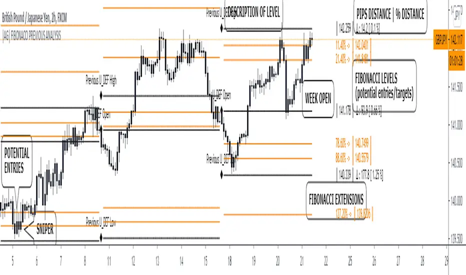
|AG| Previous Analysis█ OVERVIEW
Analysis of previous levels is one of the best strategies in order to get good entries or take profits levels. This analysis involves Monthly and Weekly Previous Levels and One User Definition Option. So u could select any period like Daily or even hours according to ur trading style. The previous levels are High and Low. And the Current (NOT PREVIOUS) open level.
This script also includes one Fibonacci Selector that will calculate the Fibbo level between previous High and Low Levels of the user selection. Almost everything could be modified in the input panel.
Input Options
A detailed explanation of input settings:
• # Of Previous
• This option leads us to select the number of previous weeks, months, or the user selection back.
• Example: If we select Previous High, Low WEEKLY so if # Of previous is one is going to be the past levels but if is 2 so consequently 2 previous levels.
• In the case of 0 is going to be the actual levels
• Fibbo & Label Selector
Here we can select the period.
• Monthly, Weekly, And User Definition is available.
• Fibonacci Selector :
• Here we could choose between different levels of Fibonacci or No_Plot Option
• Label Offset
• Here we select the amount of distance between label and actual price
• Time Start
• Here we could highlight one period START and END like one Week start day and end day.
• User Definition Value in order to be more flexible.
Interesting Code Lines:
• Fibonacci function
getFib(a, b)=>
fib1 = a + (b - a) * -0.618
fib2 = a + (b - a) * -0.270
fib3 = a + (b - a) * 0.114
fib4 = a + (b - a) * 0.214
fib5 = a + (b - a) * 0.382
fib6 = a + (b - a) * 0.500
fib7 = a + (b - a) * 0.618
fib8 = a + (b - a) * 0.786
fib9 = a + (b - a) * 0.886
ext_ = a + (b - a) * 1.270
ext1 = a + (b - a) * 1.618
• Exact Distance and % Distance
f_dist (_src, _src3) =>
float _dist = _src3 - _src
float _perc = _dist / _src3 //* 100
Difference over barsDescription:
One of my followers asked about an indicator that shows the difference between the open and a previous close and didn't find one so I wrote this one. This is similar to a momentum indicator except it offers more flexibility. While the standard momentum indicator calculates a difference between current close and a previous close (sometimes customizable to work on open, high or lows instead of close), this allows to mix and match between open, high, low and close. It also offers multiple kinds of moving averages.
Settings:
Current point of reference
Previous point of reference
Difference over how many bars?
How it works:
The indicator calculates the difference between the current point of reference and a previous (n-bars back) point of reference (where n is given by the "Difference over how many bars?").
How to use it:
find historical support lines like the 0.68 line in the cart above where in the past the indicator tends to bounce back; similarly find resistance lines like the -0.75 line in the chart (which servers as a resistance line both for the main indicator line and its moving average )
look for convergence between the price and the indicator; for example, if the price is going up and the indicator is going down a change in the price direction may be coming soon
look for the indicator crossing its moving average: moving up will signify an up trend and vice-versa
since the difference between the open and previous close (which is what the blue line in the chart shows) since to go up to 0.68 (the upper horizontal line) and down to -0.75 (the lower horizontal line) most of the time, one strategy, using options, is to to buy, right before the close of a trading day, a "long iron butterfly": buy-to-open (BTO) both a call and a put at the strike price and sell-to-open (STO) a call at a strike of around $0.68 more and sell to open a put at a strike of around $0.75 less. The STO legs should be for the next expiration and the BTO legs for the next expiration after that. This way the STO will decrease their time value faster than the BTO legs if the price stays flat (which plays to your advantage) and the BTO legs may make profit if the next day it opens away from the price at which the ticker closed the previous day (when the position was opened). The most profit is when it moves right up to one of the STO legs. This position would normally be closed next day at opening. The percentage of profit it makes is low compared to other strategies but also the percentage of the total cost at risk is also low which could potentially allow a trader to increase the lot and thus, in the end, the total profit amount may be comparable to other strategies.
Notes:
The indicator in the chart above comes with the standard options. For a more standard momentum indicator set both the current and previous reference point to the same OHLC value (such as "close").
The 0.68 and -0.75 levels are for open/close (current/previous point of reference) for ticker INTC. Obviously, other tickers will likely have other levels and you will have to find those yourself. If you use INTC but use other combination of current and previous reference points, they will have different levels as well.

Percent Calculator (Return On Investment Target Price)First and foremost: I was inspired to publish my first script after reading some of the other member's scripts -a token of my appreciation and support, Thank You.
The percent calculator is a very simple and basic indicator to use, it''s function is to simply output the target price from either the close or ones trade-entry based on a desired percent return on investment (R.O.I.).
Say you want to profit 15% from your entry: simply plug in your entry value and the number 15 into the appropriate settings and the indicator displays what the target price should be (rounded to two decimal places).
The percent calculator also goes one step further by finding the average percent return on investment over a desired interval of time (the default is 20 candles) as well as allows one to adjust the size of the price move the average percent return on investment is being calculated for.
Say you want to find the average percent return on investment for a 3 candle swing over a 200 candle interval of time: simply plug the number 200 into the interval setting and the number 3 into the price-move setting and the indicator displays what the average 3 candle swing returns on investment.
Practical Application: comparing ones desired return on investment to the average return on investment can help determine how realistic ones goals are... it's unlikely to achieve 100% return on investment if the average is only around 10% (given the parameters one is working within) but on the other hand achieving 5% return on investment is highly likely.

SIMPLE MOVING AVG 10,20,50,100,200 with RESOLUTIONThis indicator is the best than all other sma indicators.Because in just one click you can change all the resolution /time frames for all the sma .
Multitime frame analysis can be done in just one click. just change the resolution to
15 min/30 min/1hr- if you intraday trader
1D- LONG TERM INVESTORS.
Multi-timeframe analysis (MTF) is a process in which traders can view the same ticker/indicator using a higher time frame than the chart’s, for example, displaying a daily moving average on a one-hour chart in just two clicks.
How to Use this to Buy Stocks ?
The technical indicator known as the Death cross occurs when the 50-day SMA crosses below the 200-day SMA => Bearish Signal.
An opposite indicator, known as the Golden cross, occurs when the 50-day SMA crosses above the 200-day SMA => Bullish Signal.
Crossovers are one of the main moving average strategies.
1st Strategy is the first type is a price crossover, which is when the price crosses above the sma => Buy signal
when the price crosses below the sma => Sell signal
2nd Strategy is to apply two moving averages to a chart: one longer and one shorter.
When the shorter-term MA (100) crosses above the longer-term MA (200), it's a buy signal, indicates trend is shifting up.
This is known as a "Golden cross."
Meanwhile, when the shorter-term MA (100) crosses below the longer-term MA (200), it's a sell signal, indicates trend is shifting down.
This is known as a "Dead/death cross."
The time frame or length you choose for a moving average, also called the "look back period," can play a big role in how effective it is.
An MA with a short time frame will react much quicker to price changes than an MA with a long look back period. In the figure below, the 20-day moving average more closely tracks the actual price than the 100-day moving average does.
A 20-day MA = more beneficial to a shorter-term trader, since it follows the price more closely.
A 100-day MA = more beneficial to a longer-term trader.
Moving averages work quite well in strong trending conditions but poorly in choppy or ranging conditions.
use this indicator along with Price action theory and not alone.
Moving average crossovers are a popular strategy for both entries and exits. MAs can also highlight areas of potential support or resistance
Happy Trading

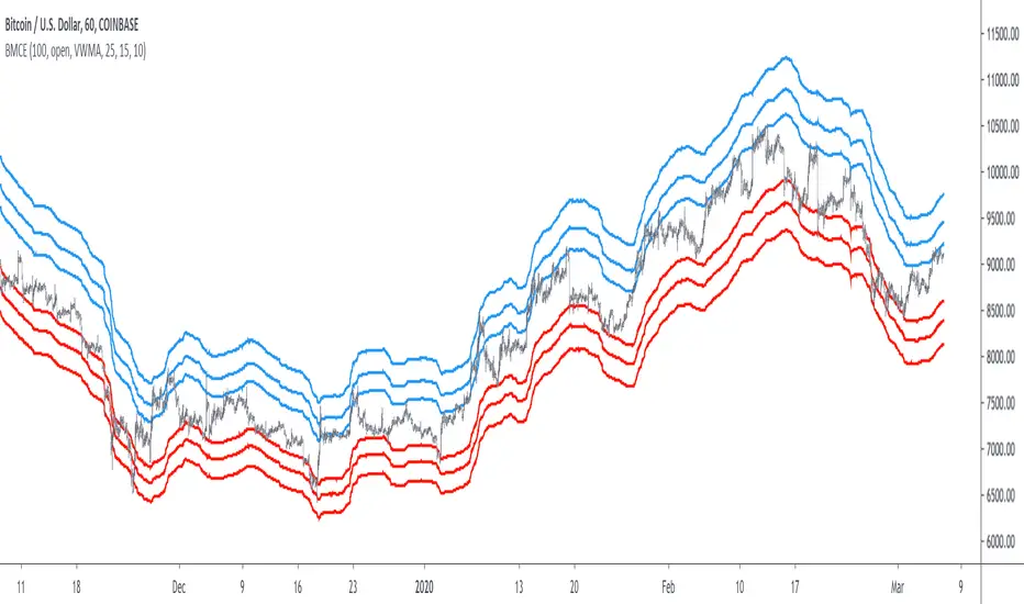
Bitcoin Margin Call Envelopes [saraphig & alexgrover]Bitcoin is the most well known digital currency, and allow two parties to make a transaction without the need of a central entity, this is why cryptocurrencies are said to be decentralized, there is no central unit in the transaction network, this can be achieved thanks to cryptography. Bitcoin is also the most traded cryptocurrency and has the largest market capitalization, this make it one of the most liquid cryptocurrency.
There has been tons of academic research studying the profitability of Bitcoin as well as its role as a safe heaven asset, with all giving mixed conclusions, some says that Bitcoin is to risky to be considered as an hedging instrument while others highlight similarities between Bitcoin and gold thus showing evidence on the usefulness of Bitcoin acting as an hedging instrument. Yet Bitcoin seems to attract more short term speculative investors rather than other ones that would use Bitcoin as an hedging instrument.
Once introduced, cryptocurrencies where of course heavily analyzed by technical analyst, and technical indicators where used by retail as well as institutional investors in order to forecast the future trends of bitcoin. I never really liked the idea of designing indicators that specifically worked for only one type of market and ever less on only one symbol. Yet the user @saraphig posted in Feb 20 an indicator called " Margin Call MovingAverage " who calculate liquidation price by using a volume weighted moving average. It took my attention and we decided to work together on a relatively more complete version that would include resistances levels.
I believe the proposed indicator might result useful to some users, the code also show a way to restrict the use of an indicator to only one symbol (line 9 to 16).
The Indicator
The indicator only work on BTCUSD, if you use another symbol you should see the following message:
The indicator plot 6 extremities, with 3 upper (resistance) extremities and 3 lower (support) extremities, each one based on the isolated margin mode liquidation price formula:
UPlp = MA/Leverage × (Leverage+1-(Leverage*0.005))
for upper extremities and:
DNlp = MA × Leverage/(Leverage+1-(Leverage*0.005))
for lower extremities.
Length control the period of the moving averages, with higher values of length increasing the probability of the price crossing an extremity. The Leverage's settings control how far away their associated extremities are from the price, with lower values of Leverage making the extremity farther away from the price, Leverage 3 control Up3 and Dn3, Leverage 2 control Up2 and Dn2, Leverage 1 control Up1 and Dn1, @saraphig recommend values for Leverage of either : 25, 20, 15, 10 ,5.
You can select 3 different types of moving average, the default moving average is the volume weighted moving average (VWMA), you can also choose a simple moving average (SMA) and the Kaufman adaptive moving average (KAMA).
Based on my understanding (which could be wrong) the original indicator aim to highlight points where margin calls might have occurred, hence the name of the indicator.
If you want a more "DSP" like description then i would say that each extremity represent a low-pass filter with a passband greater than 1 for upper extremities and lower than 1 for lower extremities, unlike bands indicators made by adding/subtracting a volatility indicator from another moving average this allow to conserve the original shape of the moving average, the downside of it being the inability to show properly on different scales.
here length = 200, on a 1h tf, each extremities are able to detect short-terms tops and bottoms. The extremity become wider when using lower time-frames.
You would then need to increase the Leverages settings, i recommend a time frame of 1h.
Conclusion
I'am not comfortable enough to make a conclusion, as i don't know the indicator that well, however i liked the original indicator posted by @saraphig and was curious about the idea behind it, studying the effect of margin calls on market liquidity as well as making indicators based on it might result a source of inspiration for other traders.
A big thanks to @saraphig who shared a lot of information about the original indicator and allowed me to post this one. I don't exclude working with him/her in the future, i invite you to follow him/her:
www.tradingview.com
Thx for reading and have a nice weekend! :3
Extended Recursive Bands - Maximum Efficiency With Extra OptionsIntroducing A New Calculation For Efficient Bands Calculation !
Here it is ! The Recursive Bands Indicator, an indicator specially created to be extremely efficient, i think you already know that calculation time is extra important in algorithmic trading, and this is the principal motivation for the creation of the proposed indicator. Originally described in my paper "Pierrefeu, Alex (2019): Recursive Bands - A New Indicator For Technical Analysis" , the indicator framework has been widely used in my previous uploaded indicators, however it would have been a shame to not upload it, however user experience being a major concern for me, i decided to add extra options, which explain the term "extended".
On The Indicator Calculation
You can skip this part if it doesn't interest you. The calculation of the indicator is based on recursion, but i want to explain the mathematical formula described in the paper.
I've seen some users trying to remake it from the calculations, however there was always something weird, and i understand, mathematical notations are always a bit weird, even myself don't always write them correctly/understand them, however this one is relatively simple to understand.
First lets explain each elements of the calculation :
α = smoothing constant, or 2/(length+1)
max/min = maximum and minimum function, max return the greatest input value while min return the lowest one, for example :
max(4,2) = 4 while min(4,2) = 2
the "||" notation mean taking the absolute value, for example : |-1| = abs(-1) = 1
The calculation after the max/min function is called the correction factor, and is the core of the indicator. The last two variables are just here to provide an initial value for upper and lower, basically when we start our calculations we will assign the value of the closing price for upper and lower.
The motivation behind using a smoothing constant in range of (0,1) was to tell the reader that the indicator is easily made adaptive, this is what i did on my adaptive trailing stop indicator by using the efficiency ratio as smoothing variable, the user can use 1/length instead of the provided calculation for alpha.
If you interested on the indicator main logic, it is actually really simple, by using upper = max(price,upper) and lower = min(price,lower) we would get the maximum/minimum price value at time t , therefore upper can only be greater or equal than its precedent value, while lower can only be lower or equal than its precedent value, in order to fix that we subtract/sum upper/lower with a value, this allow the upper band to be lower than its precedent value and lower to be greater than its precedent value, this is the role of the correction factor.
The Indicator
The indicator display one upper and one lower band, every common usages applied to bands indicators such as support/resistance, breakout, trailing stop...etc, can also be applied to this one. length control how reactive the bands are, higher values of length will make the bands cross the price less often.
In order to provide more flexibility for the user i added the option to use various methods for the calculation of the indicator, therefore the indicator can use the average true range, standard deviation, average high-low range, and one totally exclusive method specially designed for this indicator.
Classic Method
This option make the indicator use its classical calculation, this is the most efficient method of all.
Atr Method (atr)
This method use the average true range as correction factor, notice that lower values of length can still produce wide band.
Standard Deviation Method (stdev)
This method use a biased estimate of the standard deviation as correction factor.
The method produce smoother bands that converge more slowly toward the price in comparison with the classic correction factor.
Average High-Low Range Method (ahlr)
This method use the average of the high-low range as correction factor, extremely similar to the average true range.
Rising Falling Volatility (rfv) Method
A new method created for this indicator, this correction factor use the absolute prices changes when price value is greater/lower than any length past values of the price, this allow to have more boxy shaped bands, work best with greater values of length.
The bands can be in contact with this method, a possible fix in the future.
Conclusion
The recursive band indicator is one of my greatest indicators in my opinion (i would love to have yours), as you can see the idea behind it is extremely simple and allow for a super efficient band indicator, which was the original motivation behind it, in order to provide more fun for the users i also added more option for the correction factor, this allow the user to be creative and not get stuck with the original calculation.
Like the trend step indicator family we have almost ended our series on the recursive band framework, 1 more trailing stop will be added in the future, and then we'll have more "boring" stuff until i find something cool again, it shouldn't be long ;)
Thanks for reading !

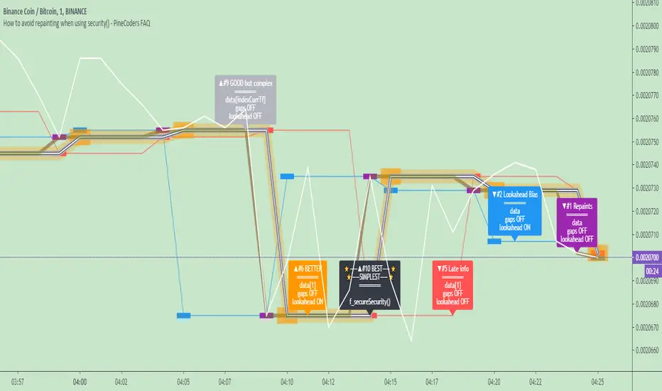
How to avoid repainting when using security() - PineCoders FAQNOTE
The non-repainting technique in this publication that relies on bar states is now deprecated, as we have identified inconsistencies that undermine its credibility as a universal solution. The outputs that use the technique are still available for reference in this publication. However, we do not endorse its usage. See this publication for more information about the current best practices for requesting HTF data and why they work.
This indicator shows how to avoid repainting when using the security() function to retrieve information from higher timeframes.
What do we mean by repainting?
Repainting is used to describe three different things, in what we’ve seen in TV members comments on indicators:
1. An indicator showing results that change during the realtime bar, whether the script is using the security() function or not, e.g., a Buy signal that goes on and then off, or a plot that changes values.
2. An indicator that uses future data not yet available on historical bars.
3. An indicator that uses a negative offset= parameter when plotting in order to plot information on past bars.
The repainting types we will be discussing here are the first two types, as the third one is intentional—sometimes even intentionally misleading when unscrupulous script writers want their strategy to look better than it is.
Let’s be clear about one thing: repainting is not caused by a bug ; it is caused by the different context between historical bars and the realtime bar, and script coders or users not taking the necessary precautions to prevent it.
Why should repainting be avoided?
Repainting matters because it affects the behavior of Pine scripts in the realtime bar, where the action happens and counts, because that is when traders (or our systems) take decisions where odds must be in our favor.
Repainting also matters because if you test a strategy on historical bars using only OHLC values, and then run that same code on the realtime bar with more than OHLC information, scripts not properly written or misconfigured alerts will alter the strategy’s behavior. At that point, you will not be running the same strategy you tested, and this invalidates your test results , which were run while not having the additional price information that is available in the realtime bar.
The realtime bar on your charts is only one bar, but it is a very important bar. Coding proper strategies and indicators on TV requires that you understand the variations in script behavior and how information available to the script varies between when the script is running on historical and realtime bars.
How does repainting occur?
Repainting happens because of something all traders instinctively crave: more information. Contrary to trader lure, more information is not always better. In the realtime bar, all TV indicators (a.k.a. studies ) execute every time price changes (i.e. every tick ). TV strategies will also behave the same way if they use the calc_on_every_tick = true parameter in their strategy() declaration statement (the parameter’s default value is false ). Pine coders must decide if they want their code to use the realtime price information as it comes in, or wait for the realtime bar to close before using the same OHLC values for that bar that would be used on historical bars.
Strategy modelers often assume that using realtime price information as it comes in the realtime bar will always improve their results. This is incorrect. More information does not necessarily improve performance because it almost always entails more noise. The extra information may or may not improve results; one cannot know until the code is run in realtime for enough time to provide data that can be analyzed and from which somewhat reliable conclusions can be derived. In any case, as was stated before, it is critical to understand that if your strategy is taking decisions on realtime tick data, you are NOT running the same strategy you tested on historical bars with OHLC values only.
How do we avoid repainting?
It comes down to using reliable information and properly configuring alerts, if you use them. Here are the main considerations:
1. If your code is using security() calls, use the syntax we propose to obtain reliable data from higher timeframes.
2. If your script is a strategy, do not use the calc_on_every_tick = true parameter unless your strategy uses previous bar information to calculate.
3. If your script is a study and is using current timeframe information that is compared to values obtained from a higher timeframe, even if you can rely on reliable higher timeframe information because you are correctly using the security() function, you still need to ensure the realtime bar’s information you use (a cross of current close over a higher timeframe MA, for example) is consistent with your backtest methodology, i.e. that your script calculates on the close of the realtime bar. If your system is using alerts, the simplest solution is to configure alerts to trigger Once Per Bar Close . If you are not using alerts, the best solution is to use information from the preceding bar. When using previous bar information, alerts can be configured to trigger Once Per Bar safely.
What does this indicator do?
It shows results for 9 different ways of using the security() function and illustrates the simplest and most effective way to avoid repainting, i.e. using security() as in the example above. To show the indicator’s lines the most clearly, price on the chart is shown with a black line rather than candlesticks. This indicator also shows how misusing security() produces repainting. All combinations of using a 0 or 1 offset to reference the series used in the security() , as well as all combinations of values for the gaps= and lookahead= parameters are shown.
The close in the call labeled “BEST” means that once security has reached the upper timeframe (1 day in our case), it will fetch the previous day’s value.
The gaps= parameter is not specified as it is off by default and that is what we need. This ensures that the value returned by security() will not contain na values on any of our chart’s bars.
The lookahead security() to use the last available value for the higher timeframe bar we are using (the previous day, in our case). This ensures that security() will return the value at the end of the higher timeframe, even if it has not occurred yet. In our case, this has no negative impact since we are requesting the previous day’s value, with has already closed.
The indicator’s Settings/Inputs allow you to set:
- The higher timeframe security() calls will use
- The source security() calls will use
- If you want identifying labels printed on the lines that have no gaps (the lines containing gaps are plotted using very thick lines that appear as horizontal blocks of one bar in length)
For the lines to be plotted, you need to be on a smaller timeframe than the one used for the security() calls.
Comments in the code explain what’s going on.
Look first. Then leap.
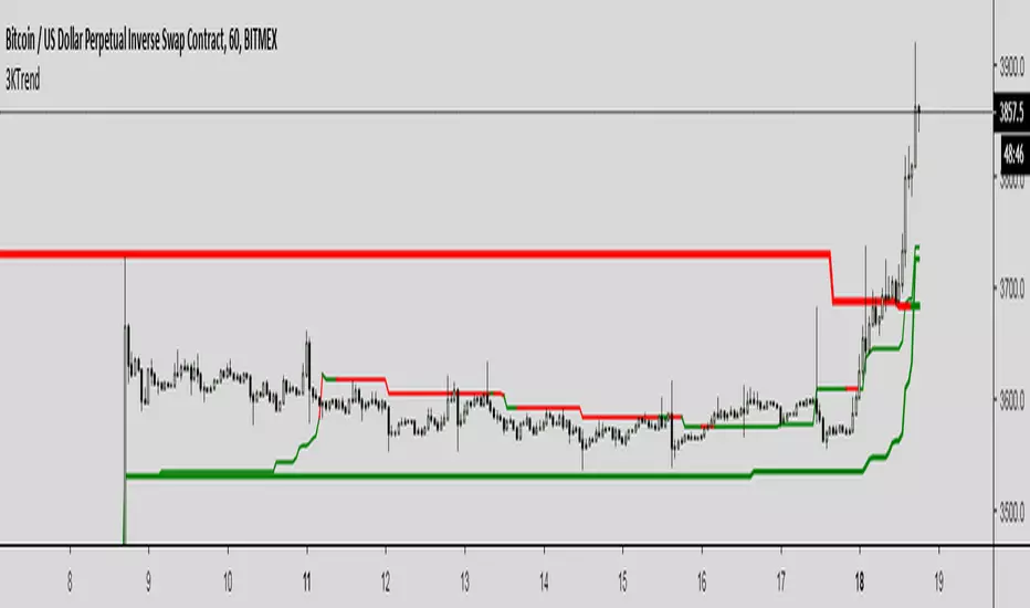
Triple Kijun Trend by SpiralmanIspired from "Oscars Simple Trend Ichimoku Kijun-sen" by CapnOscar
Script displays 3 kijun lines: one for current TF, second one emulates it for TF 4 times higher, third one for x16.
For example on 1H chart there will be 3 kijuns: one for 1H, second one for 4H (emulated), third one for 16H (emulated).
Kijuns change colors based on their position relative to price.
Kijun Sen
The base line, the slower EMA derivative, and a dynamic representation of the mean. With that said, the Kijun serves as both critical support and resistance levels for price. How does it work, and why would the Kijun be superior to commonly used moving average indicators? Fun fact: The Kijun dynamically equalizes itself to be the 50% retracement (or 0.5 Fibonacci level) of price for any given swing, and price will ALWAYS gravitate to the Kijun at some point regardless of how far above or below it is from it. By taking the median of price extremes, the Kijun accounts for volatility that other MAs or EMAs do not. A flat horizontal Kijun means that price extremes have not changed, and that the current trend losing momentum. Crypto-adjusted calculation: (highest high + lowest low) / 2 calculated over the last 60 periods.
Back to zero: Understanding seriestype: pine series basic example
time required: 10 minutes
level: medium (need to know the "array" data variable as a generic programming concept, basic Pine syntax)
tl;dr how variables and series work in Pine
Pine is an array/vector language. That's something that twists how it behaves, and how we have to think about it. A lot of misunderstandings come from forgetting this fact. This example tries to clear that concept.
First, you need to know what an array is, and how it works in a programmig language. Also, having javascript under your belt helps too. If you don't, google "javascript array basic tutorial" is your friend :)
So, in pine arrays are called "series". Every variable is an array with values for each candle in the chart. if we do:
myVar = true
this is not a constant. It is a series of values for each candle, { true, true,....., true }
In practice, the result is the same, but we can access each of the values in the series, like myVar{0}, myVar{7}, myVar{anyNumber}....
Again, it is not a constant, since you can access/modify the each value individually
so, lets show it:
plot (myVar, clolor = gray)
this plots an horizontal line of value 1 ( 1 is equal to true ) so it's all good.
On to a more usual series:
tipicalSeries = close > open ? true : false
plot(tipicalSeries, color= blue)
This gives the expected result, a tipical up and down line with values at 1 or 0. Naturally, "tipicalSeries" is an array, the "ups" and "downs" are all stored under the same variable, indexed by the candles.
In Pine, the ZERO position in the array is the last one, which corresponds to the last candle on the right. Say you have a chart with 12 candles. The close would be the closing value of what we intuitively think as first candle, the one on the left. then close ... and so on.... until close , the value of the "last" candle, the one on the right. It actually helps to start thinking of the positions backwards, counting down to zero, rocket launch style :)
And back to our series. The myVar will also be the same size, from myVar to myVar .
When we do some operation with them, something simple like
if ( myVar == tipicalSeries)
what is really happening is that internally, Pine is checking each of the indexes, as in myVar == tipicalSeries , myVar == tipicalSeries .... myVar == tipicalSeries
And we can store that stuff to check it. simply:
result = (myVar == tipicalSeries) ? true : false //yes, this is the same as tipicalSeries, but we're not in a boolean logic tut ;)
plot (result)
The reason we can plot the result is that it is an array, not a single value. The example indicator i provide shows a plot where the values are obtained from different places in the array, this line here:
mySeries3 = mySeries2 and mySeries1
this creates a series that is the result of the PREVIOUS values stored (the zero index is the one most at the right, or the "current" one), which here just causes a shift in the plotted line by one candle.
Go ahead, grab a copy of my code, try to change the indexes and see the results. Understanding this stuff is critical to go deeper into Pine :)

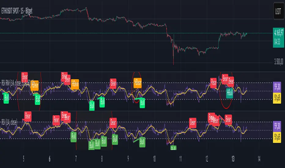
Relative Strength Index Remastered [CHE]Relative Strength Index Remastered — Enhanced RSI with robust divergence detection using price-based pivots and line-of-sight validation to reduce false signals compared to the standard RSI indicator.
Summary
RSI Remastered builds on the classic Relative Strength Index by adding a more reliable divergence detection system that relies on price pivots rather than RSI pivots alone, incorporating a line-of-sight check to ensure the RSI path between points remains clear. This approach filters out many false divergences that occur in the original RSI indicator due to its volatile pivot detection on the RSI line itself. Users benefit from clearer reversal and continuation signals, especially in noisy markets, with optional hidden divergence support for trend confirmation. The core RSI calculation and smoothing options remain familiar, but the divergence logic provides materially fewer alerts while maintaining sensitivity.
Motivation: Why this design?
The standard RSI indicator often generates misleading divergence signals because it detects pivots directly on the RSI values, which can fluctuate erratically in volatile conditions, leading to frequent false positives that confuse traders during ranging or choppy price action. RSI Remastered addresses this by shifting pivot detection to the underlying price highs and lows, which are more stable, and adding a validation step that confirms the RSI line does not cross the direct path between pivot points. This design targets the real problem of over-signaling in the original, promoting more actionable insights without altering the RSI's core momentum measurement.
What’s different vs. standard approaches?
- Reference baseline: The classical TradingView RSI indicator, which uses simple RSI-based pivot detection for divergences.
- Architecture differences:
- Pivot identification on price extremes (highs and lows) instead of RSI values, extracting RSI levels at those points for comparison.
- Addition of a line-of-sight validation that checks the RSI path bar by bar between pivots to prevent signals where the line is interrupted.
- Inclusion of hidden divergence types alongside regular ones, using the same robust framework.
- Configurable drawing of connecting lines between validated pivot RSI points for visual clarity.
- Practical effect: Charts show fewer but higher-quality divergence markers and lines, reducing clutter from the original's frequent RSI pivot triggers; this matters for avoiding whipsaws in intraday trading, where the standard version might flag dozens of invalid setups per session.
Key Comparison Aspects
Aspect: Title/Shorttitle
Original RSI: "Relative Strength Index" / "RSI"
Robust Variant: "Relative Strength Index Remastered " / "RSI RM"
Aspect: Max. Lines/Labels
Original RSI: No specification (Standard: 50/50)
Robust Variant: max_lines_count=200, max_labels_count=200 (for more lines/markers in divergences)
Aspect: RSI Calculation & Plots
Original RSI: Identical: RSI with RMA, Plots (line, bands, gradient fills)
Robust Variant: Identical: RSI with RMA, Plots (line, bands, gradient fills)
Aspect: Smoothing (MA)
Original RSI: Identical: Inputs for MA types (SMA, EMA etc.), Bollinger Bands optional
Robust Variant: Identical: Inputs for MA types (SMA, EMA etc.), Bollinger Bands optional
Aspect: Divergence Activation
Original RSI: input.bool(false, "Calculate Divergence") (disabled by default)
Robust Variant: input.bool(true, "Calculate Divergence") (enabled by default, with tooltip)
Aspect: Pivot Calculation
Original RSI: Pivots on RSI (ta.pivotlow/high on RSI values)
Robust Variant: Pivots on price (ta.pivotlow/high on low/high), RSI values then extracted
Aspect: Lookback Values
Original RSI: Fixed: lookbackLeft=5, lookbackRight=5
Robust Variant: Input: L=5 (Pivot Left), R=5 (Pivot Right), adjustable (min=1, max=50)
Aspect: Range Between Pivots
Original RSI: Fixed: rangeUpper=60, rangeLower=5 (via _inRange function)
Robust Variant: Input: rangeUpper=60 (Max Bars), rangeLower=5 (Min Bars), adjustable (min=1–6, max=100–300)
Aspect: Divergence Types
Original RSI: Only Regular Bullish/Bearish: - Bull: Price LL + RSI HL - Bear: Price HH + RSI LH
Robust Variant: Regular + Hidden (optional via showHidden=true): - Regular Bull: Price LL + RSI HL - Regular Bear: Price HH + RSI LH - Hidden Bull: Price HL + RSI LL - Hidden Bear: Price LH + RSI HH
Aspect: Validation
Original RSI: No additional check (only pivot + range check)
Robust Variant: Line-of-Sight Check: RSI line must not cross the connecting line between pivots (line_clear function with slope calculation and loop for each bar in between)
Aspect: Signals (Plots/Shapes)
Original RSI: - Plot of pivot points (if divergence) - Shapes: "Bull"/"Bear" at RSI value, offset=-5
Robust Variant: - No pivot plots, instead shapes at RSI , offset=-R (adjustable) - Shapes: "Bull"/"Bear" (Regular), "HBull"/"HBear" (Hidden) - Colors: Lime/Red (Regular), Teal/Orange (Hidden)
Aspect: Line Drawing
Original RSI: No lines
Robust Variant: Optional (showLines=true): Lines between RSI pivots (thick for regular, dashed/thin for hidden), extend=none
Aspect: Alerts
Original RSI: Only Regular Bullish/Bearish (with pivot lookback reference)
Robust Variant: Regular Bullish/Bearish + Hidden Bullish/Bearish (specific "at latest pivot low/high")
Aspect: Robustness
Original RSI: Simple, prone to false signals (RSI pivots can be volatile)
Robust Variant: Higher: Price pivots are more stable, line-of-sight filters "broken" divergences, hidden support for trend continuations
Aspect: Code Length/Structure
Original RSI: ~100 lines, simple if-blocks for bull/bear
Robust Variant: ~150 lines, extended helper functions (e.g., inRange, line_clear), var group for inputs
How it works (technical)
The indicator first computes the core RSI value based on recent price changes, separating upward and downward movements over the specified length and smoothing them to derive a momentum reading scaled between zero and one hundred. This value is then plotted in a separate pane with fixed upper and lower reference lines at seventy and thirty, along with optional gradient fills to highlight overbought and oversold zones.
For smoothing, a moving average type is applied to the RSI if enabled, with an option to add bands around it based on the variability of recent RSI values scaled by a multiplier. Divergence detection activates on confirmed price pivots: lows for bullish checks and highs for bearish. At each new pivot, the system retrieves the bar index and values (price and RSI) for the current and prior pivot, ensuring they fall within a configurable bar range to avoid unrelated points.
Comparisons then assess whether the price has made a lower low (or higher high) while the RSI at those points moves in the opposite direction—higher for bullish regular, lower for bearish regular. For hidden types, the directions reverse to capture trend strength. The line-of-sight check calculates the straight path between the two RSI points and verifies that the actual RSI values in between stay entirely above (for bullish) or below (for bearish) that path, breaking the signal if any bar violates it. Valid signals trigger shapes at the RSI level of the new pivot and optional lines connecting the points. Initialization uses built-in functions to track prior occurrences, with states persisting across bars for accurate historical comparisons. No higher timeframe data is used, so confirmation occurs after the right pivot bars close, minimizing live-bar repaints.
Parameter Guide
Length — Controls the period for measuring price momentum changes — Default: 14 — Trade-offs/Tips: Shorter values increase responsiveness but add noise and more false signals; longer smooths trends but delays entries in fast markets.
Source — Selects the price input for RSI calculation — Default: Close — Trade-offs/Tips: Use high or low for volatility focus, but close works best for most assets; mismatches can skew overbought/oversold reads.
Calculate Divergence — Enables the enhanced divergence logic — Default: True — Trade-offs/Tips: Disable for pure RSI view to save computation; essential for signal reliability over the standard method.
Type (Smoothing) — Chooses the moving average applied to RSI — Default: SMA — Trade-offs/Tips: None for raw RSI; EMA for quicker adaptation, but SMA reduces whipsaws; Bollinger Bands option adds volatility context at cost of added lines.
Length (Smoothing) — Period for the smoothing average — Default: 14 — Trade-offs/Tips: Match RSI length for consistency; shorter boosts signal speed but amplifies noise in the smoothed line.
BB StdDev — Multiplier for band width around smoothed RSI — Default: 2.0 — Trade-offs/Tips: Lower narrows bands for tighter signals, risking more touches; higher widens for fewer but stronger breakouts.
Pivot Left — Bars to the left for confirming price pivots — Default: 5 — Trade-offs/Tips: Increase for stricter pivots in noisy data, reducing signals; too high delays confirmation excessively.
Pivot Right — Bars to the right for confirming price pivots — Default: 5 — Trade-offs/Tips: Balances with left for symmetry; longer right ensures maturity but shifts signals backward.
Max Bars Between Pivots — Upper limit on distance for valid pivot pairs — Default: 60 — Trade-offs/Tips: Tighten for short-term trades to focus recent action; widen for swing setups but risks unrelated comparisons.
Min Bars Between Pivots — Lower limit to avoid clustered pivots — Default: 5 — Trade-offs/Tips: Raise to filter micro-moves; too low invites overlapping signals like the original RSI.
Detect Hidden — Includes trend-continuation hidden types — Default: True — Trade-offs/Tips: Enable for full trend analysis; disable simplifies to reversals only, akin to basic RSI.
Draw Lines — Shows connecting lines between valid pivots — Default: True — Trade-offs/Tips: Turn off for cleaner charts; helps visually confirm line-of-sight in backtests.
Reading & Interpretation
The main RSI line oscillates between zero and one hundred, crossing above fifty suggesting building momentum and below indicating weakness; touches near seventy or thirty flag potential extremes. The optional smoothed line and bands provide a filtered view—price above the upper band on the RSI pane hints at overextension. Divergence shapes appear as upward labels for bullish (lime for regular, teal for hidden) and downward for bearish (red regular, orange hidden) at the pivot's RSI level, signaling a mismatch only after validation. Connecting lines, if drawn, slope between points without RSI interference, their color matching the shape type; a dashed style denotes hidden. Fewer shapes overall compared to the standard RSI mean higher conviction, but always confirm with price structure.
Practical Workflows & Combinations
- Trend following: Enter longs on regular bullish shapes near support with higher highs in price; filter hidden bullish for pullback buys in uptrends, pairing with a rising smoothed RSI above fifty.
- Exits/Stops: Use bearish regular as reversal warnings to tighten stops; hidden bearish in downtrends confirms continuation—exit if lines show RSI crossing the path.
- Multi-asset/Multi-TF: Defaults suit forex and stocks on one-hour charts; for crypto volatility, widen pivot ranges to ten; scale min/max bars proportionally on daily for swings, avoiding the original's intraday spam.
Behavior, Constraints & Performance
Signals confirm only after the right pivot bars close, so live bars may show tentative pivots that vanish on close, unlike the standard RSI's immediate RSI-pivot triggers—plan for this delay in automation. No higher timeframe calls, so no security-related repaints. Resources include up to two hundred lines and labels for dense charts, with a loop in validation scanning up to three hundred bars between pivots, which is efficient but could slow on very long histories. Known limits: Slight lag at pivot confirmation in trending markets; volatile RSI might rarely miss fine path violations; not ideal for gap-heavy assets where pivots skip.
Sensible Defaults & Quick Tuning
Start with defaults for balanced momentum and divergence on most timeframes. For too many signals (like the original), raise pivot left/right to eight and min bars to ten to filter noise. If sluggish in trends, shorten RSI length to nine and enable EMA smoothing for faster adaptation. In high-volatility assets, widen max bars to one hundred but disable hidden to focus essentials. For clean reversal hunts, set smoothing to none and lines on.
What this indicator is—and isn’t
RSI Remastered serves as a refined momentum and divergence visualization tool, enhancing the standard RSI for better signal quality in technical analysis setups. It is not a standalone trading system, nor does it predict price moves—pair it with volume, structure breaks, and risk rules for decisions. Use alongside position sizing and broader context, not in isolation.
Disclaimer
The content provided, including all code and materials, is strictly for educational and informational purposes only. It is not intended as, and should not be interpreted as, financial advice, a recommendation to buy or sell any financial instrument, or an offer of any financial product or service. All strategies, tools, and examples discussed are provided for illustrative purposes to demonstrate coding techniques and the functionality of Pine Script within a trading context.
Any results from strategies or tools provided are hypothetical, and past performance is not indicative of future results. Trading and investing involve high risk, including the potential loss of principal, and may not be suitable for all individuals. Before making any trading decisions, please consult with a qualified financial professional to understand the risks involved.
By using this script, you acknowledge and agree that any trading decisions are made solely at your discretion and risk.
Do not use this indicator on Heikin-Ashi, Renko, Kagi, Point-and-Figure, or Range charts, as these chart types can produce unrealistic results for signal markers and alerts.
Best regards and happy trading
Chervolino
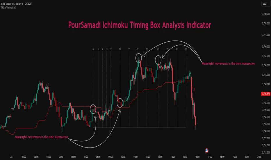
Ichimoku PourSamadi Signal [TradingFinder] KijunSen Magic Number🔵 Introduction
The Ichimoku Kinko Hyo system is one of the most comprehensive market analysis tools ever created. Developed by Goichi Hosoda, a Japanese journalist in the 1930s, its purpose was to allow traders to recognize the balance between price, time, and momentum at a single glance. (In Japanese, Ichimoku literally means “one look.”)
At the core of the system lie five key components: Tenkan-sen (Conversion Line), Kijun-sen (Baseline), Chikou Span (Lagging Line), and the two leading spans, Senkou Span A and Senkou Span B, which together form the well-known Kumo or cloud representing both temporal structure and equilibrium zones in the market.
Although Ichimoku is commonly used to identify trends and support/resistance levels, a deeper layer of time philosophy exists within it. Ichimoku was not designed solely for price analysis but equally for time analysis.
In the classical model, the numerical cycles 9, 26, 52 reflect the natural rhythm of the market originally based on the Tokyo Stock Exchange’s trading schedule in the 1930s.
These values repeat across the system’s calculations, forming the foundation of Ichimoku’s time symmetry where price and time ultimately seek equilibrium.
In recent years, modern analysts have explored new approaches to extract time-based turning points from Ichimoku’s structure. One such approach is the analysis of flat segments on the Kijun-sen and Senkou B lines.
Whenever one of these lines remains flat for a period, it signals temporary balance between buyers and sellers; when the flat breaks, the market exits equilibrium and a new cycle begins.
This indicator is built precisely upon that philosophy. Following the timing methodology introduced by M.A. Poursamadi, the focus shifts away from price signals and line crossovers toward identifying flat periods on Kijun-sen (period 52) as time anchors.
From the first candle that changes the line’s slope, the tool begins a temporal count using a fixed sequence of key numbers: 5, 9, 13, 17, 26, 35, 43, 52, 63, 72, 81, 90.
Derived from both classical Ichimoku cycles and empirical testing, these numbers mark potential timing nodes where a market wave may end, a correction may begin, or a new leg may form.
Thus, this method serves not merely as another Ichimoku tool but as a temporal metronome for market structure a way to visualize moments when the market is ready to change rhythm, often before candles reveal it.
🔵 How to Use
The Kijun Timing BoX is built entirely on Ichimoku’s concept of time analysis.
Its core idea is that within every flat segment of the Kijun-sen, the market enters a temporary balance between opposing forces.
When that flat breaks, a new time cycle begins. From that first breakout candle, the indicator starts counting forward through the predefined time sequence(5, 9, 13, 17, 26, 35, 43, 52, 63, 72, 81, 90).
This counting framework creates a temporal map of market behavior, where each number represents an area where meaningful price fluctuations often occur.
A “meaningful fluctuation” does not necessarily imply reversal or continuation; rather, it marks a moment when the market’s internal energy balance shifts, typically visible as noticeable reactions on lower timeframes.
🟣 Identifying the Anchor Point
The first step is recognizing a valid flat zone on the Kijun-sen.
When this line remains flat for several candles and then changes slope, the indicator marks that bar as the Anchor, initiating the time count.
From that point onward, vertical gray lines appear at each interval in the key-number sequence, visualizing the time nodes ahead.
🟣 Reading the Timing Lines
Each numbered line represents a timing node a temporal point where a change in price rhythm is statistically more likely to occur.
At these nodes, the market may :
Enter a consolidation or minor correction phase.
Develop range-bound movement.
Or simply alter the speed and intensity of its move.
These behaviors do not imply a specific direction; they only highlight zones where time-based activity tends to cluster, giving traders a clearer view of cyclical rhythm.
🟣 Applying Time Analysis
The indicator’s primary use is to observe temporal order, not to predict price direction.
By tracking the distance between Anchors and the reactions that appear near major timing lines, traders can empirically identify each market’s characteristic rhythm—its own time DNA.
For example, one asset may consistently show significant fluctuations around the 13- and 26-bar marks,while another might react closer to 9 or 52. Recognizing such patterns helps traders understand how long typical cycles last before new phases of volatility emerge.
🟣 Combining with Other Tools
The indicator does not generate buy/sell signals on its own.
Its best use is in combination with price- or structure-based methods, to see whether meaningful price reactions occur around the same timing nodes.
In practice, it helps distinguish structured time-based fluctuations from random, noise-driven moves an insight often overlooked in conventional market analysis.
🔵 Settings
🟣 Logical Settings
KijunSen Period : Defines the baseline period used for timing analysis. Default = 52. It is the main line for detecting flats and generating time anchors.
Flat Event Filter : Controls how flat segments are validated before triggering a new timing event.
All : Every flat triggers a new Timing Box.
Automatic : Only flats longer than the historical average are used (recommended).
Custom : User manually defines the minimum flat length via Custom Count.
Update Timing Analysis BoX Per Event : If enabled, a new Timing Box is drawn each time a new flat event occurs. If disabled, the box completes its 90-bar window before refreshing.
🟣 Ichimoku Settings
TenkanSen Period : Defines the period for the Conversion Line (Tenkan-sen). Default = 9.
KijunSen Period : Sets the standard Ichimoku baseline (not the timing line). Default = 26.
Span B Period : Defines the period for Senkou Span B, the slower cloud boundary. Default = 52.
Shift Lines : Offsets cloud projection into the future. Default = 26.
🟣 Display Settings
Users can show or hide all Ichimoku lines Tenkan-sen, Kijun-sen, Chikou Span, Span A, and Span B as well as the Ichimoku Cloud.
They can also customize the color of each element to match personal chart preferences and improve visibility.
🔵 Conclusion
This analytical approach transforms Ichimoku’s time philosophy into a visual and measurable framework. A flat Kijun-sen represents a moment of market equilibrium; when its slope shifts, a new temporal cycle begins.
The purpose is not to forecast price direction but to highlight periods when meaningful fluctuations are more likely to develop.
Through this perspective, traders can observe the hidden rhythm of market time and expand their analysis beyond price into a broader time-cycle dimension.
Ultimately, the method revives Ichimoku’s original principle: the market can only be truly understood through the simultaneous harmony of price, time, and balance.
ATR Regime Study [CHE] ATR Regime Study — ATR percentile regimes with clear bands, table and live label
Summary
This study classifies volatility into five regimes by converting ATR into a percentile rank over a rolling window, plotted on a standardized scale between zero and one hundred. Colored bands mark regime thresholds, while a compact table and an optional label report the current percentile and regime. The standardized scale makes symbols and timeframes easier to compare than raw ATR values. Implemented in Pine v6 as a separate pane (overlay set to false), it is a context tool to adapt tactics and risk handling to the prevailing volatility environment.
Motivation: Why this design?
Raw ATR varies with price scale and asset characteristics, which makes regime comparison inconsistent and leads to poor transfer of settings across symbols and timeframes. The core idea is to transform ATR into a percentile rank within a user-defined lookback, then map it into discrete regimes. This yields a stable, interpretable context signal that shifts slower than raw ATR while still responding to genuine volatility changes.
What’s different vs. standard approaches?
Reference baseline: Traditional ATR plots or ATR bands using fixed multipliers.
Architecture differences:
Percentile ranking of ATR within a rolling window.
Five discrete regimes with fixed thresholds at ninety, seventy, thirty, and ten.
Visual fills between thresholds plus a live table and a last-bar label.
Practical effect: You read a single normalized line between zero and one hundred with consistent thresholds. This improves cross-asset comparison and makes regime shifts obvious at a glance.
How it works (technical)
The script computes ATR over a configurable length, then converts that series to a percentile rank over a configurable number of bars. The percentile is naturally scaled and limited between zero and one hundred. That value is mapped to one of five regimes: above ninety (Extreme), between seventy and ninety (Elevated), between thirty and seventy (Normal), between ten and thirty (Calm), and below ten (Squeeze). Horizontal guide lines mark the thresholds, and fills shade the regions. A table is created once and updated on each bar to show regime definitions and highlight the current row. An optional label on the last bar displays the current percentile and regime. No higher-timeframe requests are used, so repaint risk is limited to normal live-bar fluctuation until the bar closes.
Parameter Guide
ATR length — Effect: Controls how fast ATR reacts to new ranges. Default: fourteen. Trade-offs/Tips: Increase to reduce noise in choppy markets; decrease to react faster during regime changes.
Percentile window (bars) — Effect: Number of bars used for the percentile ranking. Default: two hundred fifty-two. Trade-offs/Tips: Larger windows stabilize the percentile but slow adaptation after structural regime shifts; smaller windows adapt faster but may flip more often.
Table › Show — Effect: Toggles the regime overview table. Default: enabled. Trade-offs/Tips: Disable on constrained layouts to reduce visual clutter.
Table › Position — Effect: Anchors the table in a chart corner. Default: Top Right. Trade-offs/Tips: Choose a corner that avoids overlapping other panels or drawings.
Label › Show — Effect: Toggles a last-bar label with current percentile and regime. Default: enabled. Trade-offs/Tips: Useful for quick reads; disable if it obscures other annotations.
Reading & Interpretation
The white line shows ATR percentile between zero and one hundred. Crossing above seventy signals an elevated volatility environment; above ninety indicates event-driven extremes. Between thirty and seventy represents typical conditions. Between ten and thirty indicates calm conditions that often suit mean reversion. Below ten reflects compression, where breakout probability often increases. The colored bands visually reinforce these ranges. The table summarizes regime definitions and highlights the current state. The last-bar label mirrors the current percentile and regime for quick inspection.
Practical Workflows & Combinations
Trend following: Prefer continuation tactics when the percentile holds in the Normal or Elevated bands and structure confirms higher highs and higher lows. Consider wider stops and partial position sizing as percentile rises.
Mean reversion: Favor fades in Calm regimes within defined ranges; use structure filters and time-of-day constraints to avoid low-liquidity whipsaws.
Breakout preparation: Track compressions below ten; plan entries only with structure confirmation and risk caps, since compressions can persist.
Multi-asset/Multi-TF: Defaults travel well on daily charts. For intraday, reduce the percentile window to align with session dynamics. Combine with trend or market structure tools for confirmation.
Behavior, Constraints & Performance
Repaint/confirmation: The percentile updates during live bars and stabilizes on close; closed bars do not repaint.
security/HTF: Not used. If you add higher-timeframe aggregation externally, account for standard repaint caveats.
Resources: Declared maximum bars back is two thousand; limits for lines and labels are five hundred each. A short loop updates the table rows; arrays are used for table content only.
Known limits: Regime boundaries are fixed; assets with persistent volatility shifts may require window retuning. Low-liquidity periods and gaps can produce abrupt percentile changes. ATR is direction-agnostic and should be paired with trend or structure context.
Sensible Defaults & Quick Tuning
Start with ATR length fourteen and percentile window two hundred fifty-two on daily charts.
Too many flips: Increase ATR length or increase the percentile window.
Too sluggish: Decrease the percentile window or reduce ATR length.
Intraday noise: Keep ATR length moderate and reduce the window to a session-appropriate size; optionally hide the label to declutter.
Compressed markets: Maintain defaults but rely more on structure and volume filters before acting.
What this indicator is—and isn’t
This is a volatility regime context layer that standardizes ATR into interpretable regimes. It is not a complete trading system, not predictive, and not a stand-alone entry signal. Use it alongside structure analysis, confirmation tools, and disciplined risk management.
Disclaimer
The content provided, including all code and materials, is strictly for educational and informational purposes only. It is not intended as, and should not be interpreted as, financial advice, a recommendation to buy or sell any financial instrument, or an offer of any financial product or service. All strategies, tools, and examples discussed are provided for illustrative purposes to demonstrate coding techniques and the functionality of Pine Script within a trading context.
Any results from strategies or tools provided are hypothetical, and past performance is not indicative of future results. Trading and investing involve high risk, including the potential loss of principal, and may not be suitable for all individuals. Before making any trading decisions, please consult with a qualified financial professional to understand the risks involved.
By using this script, you acknowledge and agree that any trading decisions are made solely at your discretion and risk.
Best regards and happy trading
Chervolino

Cumulative Returns by Session [BackQuant]Cumulative Returns by Session
What this is
This tool breaks the trading day into three user-defined sessions and tracks how much each session contributes to return, volatility, and volume. It then aggregates results over a rolling window so you can see which session has been pulling its weight, how streaky each session has been, and how sessions relate to one another through a compact correlation heatmap.
We’ve also given the functionality for the user to use a simplified table, just by switching off all settings they are not interested in.
How it works
1) Session segmentation
You define APAC, EU, and US sessions with explicit hours and time zones. The script detects when each session starts and ends on every intraday bar and records its open, intraday high and low, close, and summed volume.
2) Per-session math
At each session end the script computes:
Return — either Percent: (Close−Open)÷Open×100(Close − Open) ÷ Open × 100(Close−Open)÷Open×100 or Points: (Close−Open)(Close − Open)(Close−Open), based on your selection.
Volatility — either Range: (High−Low)÷Open×100(High − Low) ÷ Open × 100(High−Low)÷Open×100 or ATR scaled by price: ATR÷Open×100ATR ÷ Open × 100ATR÷Open×100.
Volume — total volume transacted during that session.
3) Storage and lookback
Each day’s three session stats are stored as a row. You choose how many recent sessions to keep in memory. The script then:
Builds cumulative returns for APAC, EU, US across the lookback.
Computes averages, win rates, and a Sharpe-like ratio avgreturn÷avgvolatilityavg return ÷ avg volatilityavgreturn÷avgvolatility per session.
Tracks streaks of positive or negative sessions to show momentum.
Tracks drawdowns on cumulative returns to show worst runs from peak.
Computes rolling means over a short window for short-term drift.
4) Correlation heatmap
Using the stored arrays of session returns, the script calculates Pearson correlations between APAC–EU, APAC–US, and EU–US, and colors the matrix by strength and sign so you can spot coupling or decoupling at a glance.
What it plots
Three lines: cumulative return for APAC, EU, US over the chosen lookback.
Zero reference line for orientation.
A statistics table with cumulative %, average %, positive session rate, and optional columns for volatility, average volume, max drawdown, current streak, return-to-vol ratio, and rolling average.
A small correlation heatmap table showing APAC, EU, US cross-session correlations.
How to use it
Pick the asset — leave Custom Instrument empty to use the chart symbol, or point to another symbol for cross-asset studies.
Set your sessions and time zones — defaults approximate APAC, EU, and US hours, but you can align them to exchange times or your workflow.
Choose calculation modes — Percent vs Points for return, Range vs ATR for volatility. Points are convenient for futures and fixed-tick assets, Percent is comparable across symbols.
Decide the lookback — more sessions smooths lines and stats; fewer sessions makes the tool more reactive.
Toggle analytics — add volatility, volume, drawdown, streaks, Sharpe-like ratio, rolling averages, and the correlation table as needed.
Why session attribution helps
Different sessions are driven by different flows. Asia often sets the overnight tone, Europe adds liquidity and direction changes, and the US session can dominate range expansion. Separating contributions by session helps you:
Identify which session has been the main driver of net trend.
Measure whether volatility or volume is concentrated in a specific window.
See if one session’s gains are consistently given back in another.
Adapt tactics: fade during a mean-reverting session, press during a trending session.
Reading the tables
Cumulative % — sum of session returns over the lookback. The sign and slope tell you who is carrying the move.
Avg Return % and Positive Sessions % — direction and hit rate. A low average but high hit rate implies many small moves; the reverse implies occasional big swings.
Avg Volatility % — typical intrabars range for that session. Compare with Avg Return to judge efficiency.
Return/Vol Ratio — return per unit of volatility. Higher is better for stability.
Max Drawdown % — worst cumulative give-back within the lookback. A quick way to spot riskiness by session.
Current Streak — consecutive up or down sessions. Useful for mean-reversion or regime awareness.
Rolling Avg % — short-window drift indicator to catch recent turnarounds.
Correlation matrix — green clusters indicate sessions tending to move together; red indicates offsetting behavior.
Settings overview
Basic
Number of Sessions — how many recent days to include.
Custom Instrument — analyze another ticker while staying on your current chart.
Session Configuration and Times
Enable or hide APAC, EU, US rows.
Set hours per session and the specific time zone for each.
Calculation Methods
Return Calculation — Percent or Points.
Volatility Calculation — Range or ATR; ATR Length when applicable.
Advanced Analytics
Correlation, Drawdown, Momentum, Sharpe-like ratio, Rolling Statistics, Rolling Period.
Display Options and Colors
Show Statistics Table and its position.
Toggle columns for Volatility and Volume.
Pick individual colors for each session line and row accents.
Common applications
Session bias mapping — find which window tends to trend in your market and plan exposure accordingly.
Strategy scheduling — allocate attention or risk to the session with the best return-to-vol ratio.
News and macro awareness — see if correlation rises around central bank cycles or major data releases.
Cross-asset monitoring — set the Custom Instrument to a driver (index future, DXY, yields) to see if your symbol reacts in a particular session.
Notes
This indicator works on intraday charts, since sessions are defined within a day. If you change session clocks or time zones, give the script a few bars to accumulate fresh rows. Percent vs Points and Range vs ATR choices affect comparability across assets, so be consistent when comparing symbols.
Session context is one of the simplest ways to explain a messy tape. By separating the day into three windows and scoring each one on return, volatility, and consistency, this tool shows not just where price ended up but when and how it got there. Use the cumulative lines to spot the steady driver, read the table to judge quality and risk, and glance at the heatmap to learn whether the sessions are amplifying or canceling one another. Adjust the hours to your market and let the data tell you which session deserves your focus.
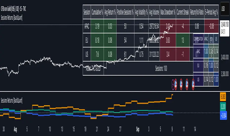
cd_SMT_Sweep_CISD_CxGeneral
This indicator is designed to show trading opportunities after sweeps of higher timeframe (HTF) highs/lows and, if available, Smart Money Technique (SMT) divergence with a correlated asset, followed by confirmation from a lower timeframe change in state delivery (CISD).
Users can track SMT, Sweep, and CISD levels across nine different timeframes.
________________________________________
Usage and Details
Commonly correlated timeframes are available in the menu by default. Users can also enter other compatible timeframes manually if necessary.
The indicator output is presented as:
• A summary table
• Display on HTF candles
• CISD levels shown as lines
Users can disable any of these from the menu.
Presentations of selected timeframes are displayed only if they are greater than or equal to the active chart timeframe.
From the Show/Hide section, you can control the display of:
• SMT table
• Sweep table
• HTF candles
• CISD levels
• HTF boxes aligned with the active timeframe
________________________________________
SMT Analysis
To receive analysis, users must enter correlated assets in the menu (or adjust them as needed).
If asset X is paired with correlated asset Y, then a separate entry for Y correlated with X is not required.
Four correlation pairs are included by default. Users should check them according to their broker/exchange or define new ones.
Checkboxes at the beginning of each row allow activation/deactivation of pairs.
SMT analysis is performed on the last three candles of each selected HTF.
If one asset makes a new high while the correlated one does not (or one makes a new low while the other does not), this is considered SMT and will be displayed both in the table and on the chart.
Charts without defined correlated assets will not display an SMT table.
________________________________________
Sweep Analysis
For the selected timeframes, the current candle is compared with the previous one.
If price violates the previous level and then pulls back behind it, this is considered a sweep. It is displayed in both the table and on the chart.
Within correlated pairs, the analysis is done separately and shown only in the table.
Example with correlated and non-correlated pairs:
• In the table, X = false, ✓ = true.
• The Sweep Table has two columns for Bullish and Bearish results.
• For correlated pairs, both values appear side by side.
• For undefined pairs, only the active asset is shown.
Example 1: EURUSD and GBPUSD pair
• If both sweep → ✓ ✓
• If one sweeps, the other does not → ✓ X
• If neither sweeps → X X
Example 2: AUDUSD with no correlated pair defined
• If sweep → ✓
• If no sweep → X
________________________________________
HTF Candles
For every HTF enabled by the user, the last three candles (including the current one) are shown on the chart.
SMT and sweep signals are marked where applicable.
________________________________________
CISD Levels
For the selected timeframes, bullish and bearish CISD levels are plotted on the chart.
________________________________________
HTF Boxes
HTF boxes aligned with the active timeframe are displayed on the chart.
Box border colors change according to whether the active HTF candle is bullish or bearish.
________________________________________
How to Read the Chart?
Let’s break down the example below:
• Active asset: Nasdaq
• Correlated asset: US500 (defined in the menu, confirmed in the table bottom row)
• Active timeframe: H1 → therefore, the HTF box is shown for Daily
• Since a correlated pair is defined, the indicator runs both SMT and Sweep analysis for the selected timeframes. Without correlation, only Sweep analysis would be shown.
Table is prepared for H1 and higher timeframes (as per user selection and active TF).
Observations:
• SMT side → H1 timeframe shows a bearish warning
• Sweep side → Bearish column shows X and ✓
o X → no sweep on Nasdaq
o ✓ → sweep on US500
Meaning: US500 made a new high (+ sweep) while Nasdaq did not → SMT formed.
The last column of the table shows the compatible LTF for confirmation.
For H1, it suggests checking the 5m timeframe.
On the chart:
• CISD levels for selected timeframes are drawn
• SMT line is marked on H1 candles
• Next step: move to 5m chart for CISD confirmation before trading (with other confluences).
Similarly, the Daily row in the table shows a Bullish Sweep on US500.
________________________________________
Alerts
Two alert options are available:
1. Activate Alert (SMT + Sweep):
Triggers if both SMT and Sweep occur in the selected timeframes. (Classic option)
2. Activate Alert (Sweep + Sweep):
Triggers if sweeps occur in both assets of a correlated pair at the same timeframe.
Interpretation:
If SMT + Sweep are already present on higher timeframes, and simultaneous sweeps appear on lower timeframes, this may indicate a strong directional move.
Of course, this must be validated with CISD and other confluences.
________________________________________
HTF CISD Levels
Although CISD levels act as confirmation levels in their own timeframe, observing how price reacts to HTF CISD levels can provide valuable insights for intraday analysis.
POIs overlapping with these levels may be higher priority.
________________________________________
What’s Next in Future Versions?
• Completed CISD confirmations
• Additional alert options
• Plus your feedback and suggestions
________________________________________
Final Note
I’ll be happy to hear your opinions and feedback.
Happy trading!
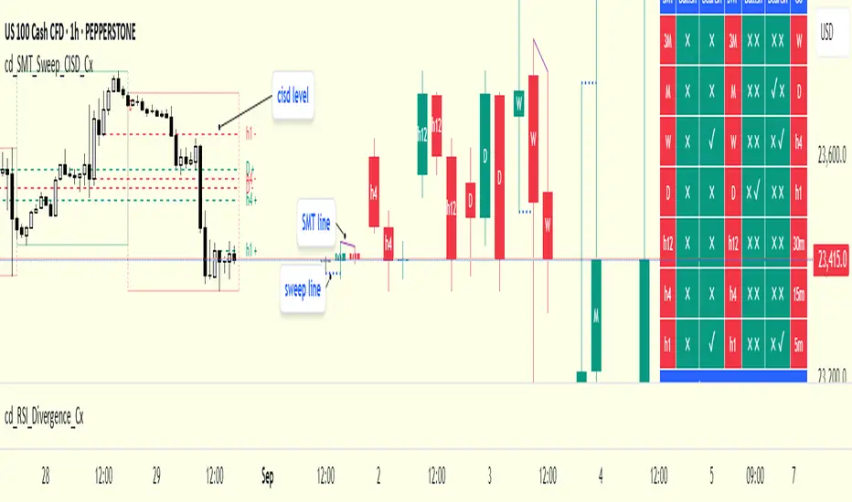
CleanBreak Lines (Break + First Retest)CleanBreak lines draws one robust support line (green) from swing lows and one robust resistance line (red) from swing highs, then optionally signals a confirmed break and the first clean retest back to that line. Lines are scored with a transparent W-Score (0–100) so traders can judge quality at a glance. The script is non-repainting and uses only confirmed bar data.
What it does
Auto-builds two trendlines that aim to represent meaningful support and resistance.
Uses a median-based slope so outliers and single spikes do not distort the line.
Computes a W-Score per line from three things: touches, span (how long it held), and respect (staying on the correct side).
Optionally triggers a single, tightly-gated signal on Break + First Retest.
How it works (plain English)
Detect recent swing highs and swing lows.
Fit one line through highs and one through lows using a robust, median-style slope estimate.
Score each line: more clean touches and longer span raise the W-Score; frequent violations lower it.
A break requires a candle close beyond the line by a small ATR margin.
A first retest requires price to come back to the line within a limited number of bars and hold on close.
A single arrow may print on that confirmed retest, with optional alerts.
What it is not
Not a prediction model and not a promises-of-profit tool.
Not a multi-signal spammer: by design it aims to allow one retest entry per break.
Not a regression channel or machine-learning system.
How to use
At a glance: treat the green line as candidate support and the red line as candidate resistance.
Conservative approach: wait for a break on close and then the first retest to hold; use the arrow as a prompt, not a command.
Context-only mode: hide arrows in Style if you want the lines and W-Score only.
Inputs (brief)
Core: Swing Length, Max Pivots, Min Touches, Min Span Bars.
Scoring: Touches Max (cap), Weights for touches vs span, Min W-Score to arm.
Break and Retest: Break Margin x ATR, Retest Tolerance x ATR, Retest Window (bars).
Visuals: Show Labels, Show Table, Line Width, Fade When Refit.
Recommended presets
Cleaner, fewer signals: Min Touches 4–5, Min Span Bars 100–150, Min W-Score 70–80, Break Margin 0.40–0.60 ATR, Retest Tolerance 0.10–0.15 ATR, Retest Window 8–12 bars.
Lines-only: keep defaults and uncheck the two plotshapes in Style.
Alerts
CB Long Retest: break above the red line and first retest holds.
CB Short Retest: break below the green line and first retest holds.
Use “Once per bar close” for consistency.
On-chart table (if enabled)
RES / SUP: W-Score and distance from price in ATR terms.
Status: “Waiting Long RT”, “Waiting Short RT”, or “Idle”.
Thresholds: MinScore and Retest bars for quick context.
Timeframes
Works well on 1h to 1D. On very low timeframes, raise Break Margin x ATR to reduce whipsaw effects. On higher timeframes, increase Min Touches and Min Span Bars.
Non-repainting policy
All logic uses confirmed pivots and confirmed bar closes.
Breaks and retests are validated on close; alerts reference only confirmed conditions.
No lookahead in any request.security call.
Original implementation focused on a median-based robust slope for auto trendlines, plus a transparent W-Score and a single retest gate.
Disclosure
This script is for education and charting. It does not guarantee outcomes, and past behavior does not imply future results. Always validate on historical data and practice risk management.

+ ATR Table and BracketsHi, all. I'm back with a new indicator—one I firmly believe could be one of the most valuable indicators you keep in your indicator toolshed—based around true range.
This is a simple, streamlined indicator utilizing true range and average true range that will help any trader with stoploss, trailing stoploss, and take-profit placement—things that I know many traders use average true range for. It could also be useful for trade entries as well, depending on the trader's style.
Typically, most traders (or at least what I've seen recommended across websites, video tutorials on YouTube, etc.) are taught to simply take the ATR number and use that, and possibly some sort of multiplier, as your stoploss and take-profit. This is fine, but I thought that it might be possible to dive a bit deeper into these values. Because an average is a combination of values, some higher, some lower, and we often see ATR spikes during periods of high volatility, I thought wouldn't it be useful to know what value those ATR spikes are, and how do they relate to the ATR? Then I thought to myself, well, what about the most volatile candle within that ATR (the candle with the greatest true range)? Couldn't knowing that value be useful to a trader? So then the idea of a table displaying these values, along with the ATR and the ATR times some multiplier number, would be a useful, simple way to display this information. That's what we have here.
The table is made up of two columns, one with the name of the metric being measured, and the other with its value. That's it. Simple.
As nice as this was, I thought an additional, great, and perhaps better, way to visualize this information would be in the form of brackets extending from the current bar. These are simply lines/labels plotted at the price values of the ATR, ATR times X, highest ATR, highest ATR times X, and highest TR value. These labels supply the actual values of the ATR, etc., but may also display the price if you should choose (both of these values are toggleable in the 'Inputs' section of the indicator.). Additionally, you can choose to display none of these labels, or all five if you wish (leaves the chart a bit cluttered, as shown in the image below), though I suspect you'll determine your preferences for which information you'd like to see and which not.
Chart with all five lines/labels displayed. I adjusted the ATRX value to 3 just to make the screenshot as legible as possible. Default is set to 1.5. As you can see, the label doesn't show the multiplier number, but the table does.
Here's a screenshot of the labels showing the price in addition to the value of the ATR, set to "Previous Closing Price," (see next paragraph for what that means) and highest TR. Personally, I don't see the value in the displaying the price, but I thought some people might want that. It's not available in the table as of now, but perhaps if I get enough requests for it I will add it.
That's basically it, but one last detail I need to go over is the dropdown box labeled "Bar Value ATR Levels are Oriented To." Firstly, this has no effect on Highest ATR, Highest ATRX, and Highest TR levels. Those are based on the ATR up to the last closed candle, meaning they aren't including the value of the currently open candle (this would be useless). However, knowing that different traders trade different ways it seemed to me prudent to allow for traders to select which opening or closing value the trader wishes to have the ATR brackets based on. For example, as someone who has consumed much No Nonsense Forex content I know that traders are urged to enter their trades in the last fifteen minutes of the trading day because the ATR is unlikely to change significantly in that period (ATR being the centerpiece of NNFX money management), so one of three selections here is to plot the brackets based on the ATR's inclusion of this value (this of course means the brackets will move while the candle is still open). The other options are to set the brackets to the current opening price, or the previous closing price. Depending on what you're trading many times these prices are virtually identical, but sometimes price gaps (stocks in particular), so, wanting your brackets placed relative to the previous close as opposed to the current open might be preferable for some traders.
And that's it. I really hope you guys like this indicator. I haven't seen anything closely similar to it on TradingView, and I think it will be something you all will find incredibly handy.
Please enjoy!
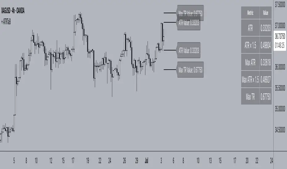
Color█ OVERVIEW
This library is a Pine Script® programming tool for advanced color processing. It provides a comprehensive set of functions for specifying and analyzing colors in various color spaces, mixing and manipulating colors, calculating custom gradients and schemes, detecting contrast, and converting colors to or from hexadecimal strings.
█ CONCEPTS
Color
Color refers to how we interpret light of different wavelengths in the visible spectrum . The colors we see from an object represent the light wavelengths that it reflects, emits, or transmits toward our eyes. Some colors, such as blue and red, correspond directly to parts of the spectrum. Others, such as magenta, arise from a combination of wavelengths to which our minds assign a single color.
The human interpretation of color lends itself to many uses in our world. In the context of financial data analysis, the effective use of color helps transform raw data into insights that users can understand at a glance. For example, colors can categorize series, signal market conditions and sessions, and emphasize patterns or relationships in data.
Color models and spaces
A color model is a general mathematical framework that describes colors using sets of numbers. A color space is an implementation of a specific color model that defines an exact range (gamut) of reproducible colors based on a set of primary colors , a reference white point , and sometimes additional parameters such as viewing conditions.
There are numerous different color spaces — each describing the characteristics of color in unique ways. Different spaces carry different advantages, depending on the application. Below, we provide a brief overview of the concepts underlying the color spaces supported by this library.
RGB
RGB is one of the most well-known color models. It represents color as an additive mixture of three primary colors — red, green, and blue lights — with various intensities. Each cone cell in the human eye responds more strongly to one of the three primaries, and the average person interprets the combination of these lights as a distinct color (e.g., pure red + pure green = yellow).
The sRGB color space is the most common RGB implementation. Developed by HP and Microsoft in the 1990s, sRGB provided a standardized baseline for representing color across CRT monitors of the era, which produced brightness levels that did not increase linearly with the input signal. To match displays and optimize brightness encoding for human sensitivity, sRGB applied a nonlinear transformation to linear RGB signals, often referred to as gamma correction . The result produced more visually pleasing outputs while maintaining a simple encoding. As such, sRGB quickly became a standard for digital color representation across devices and the web. To this day, it remains the default color space for most web-based content.
TradingView charts and Pine Script `color.*` built-ins process color data in sRGB. The red, green, and blue channels range from 0 to 255, where 0 represents no intensity, and 255 represents maximum intensity. Each combination of red, green, and blue values represents a distinct color, resulting in a total of 16,777,216 displayable colors.
CIE XYZ and xyY
The XYZ color space, developed by the International Commission on Illumination (CIE) in 1931, aims to describe all color sensations that a typical human can perceive. It is a cornerstone of color science, forming the basis for many color spaces used today. XYZ, and the derived xyY space, provide a universal representation of color that is not tethered to a particular display. Many widely used color spaces, including sRGB, are defined relative to XYZ or derived from it.
The CIE built the color space based on a series of experiments in which people matched colors they perceived from mixtures of lights. From these experiments, the CIE developed color-matching functions to calculate three components — X, Y, and Z — which together aim to describe a standard observer's response to visible light. X represents a weighted response to light across the color spectrum, with the highest contribution from long wavelengths (e.g., red). Y represents a weighted response to medium wavelengths (e.g., green), and it corresponds to a color's relative luminance (i.e., brightness). Z represents a weighted response to short wavelengths (e.g., blue).
From the XYZ space, the CIE developed the xyY chromaticity space, which separates a color's chromaticity (hue and colorfulness) from luminance. The CIE used this space to define the CIE 1931 chromaticity diagram , which represents the full range of visible colors at a given luminance. In color science and lighting design, xyY is a common means for specifying colors and visualizing the supported ranges of other color spaces.
CIELAB and Oklab
The CIELAB (L*a*b*) color space, derived from XYZ by the CIE in 1976, expresses colors based on opponent process theory. The L* component represents perceived lightness, and the a* and b* components represent the balance between opposing unique colors. The a* value specifies the balance between green and red , and the b* value specifies the balance between blue and yellow .
The primary intention of CIELAB was to provide a perceptually uniform color space, where fixed-size steps through the space correspond to uniform perceived changes in color. Although relatively uniform, the color space has been found to exhibit some non-uniformities, particularly in the blue part of the color spectrum. Regardless, modern applications often use CIELAB to estimate perceived color differences and calculate smooth color gradients.
In 2020, a new LAB-oriented color space, Oklab , was introduced by Björn Ottosson as an attempt to rectify the non-uniformities of other perceptual color spaces. Similar to CIELAB, the L value in Oklab represents perceived lightness, and the a and b values represent the balance between opposing unique colors. Oklab has gained widespread adoption as a perceptual space for color processing, with support in the latest CSS Color specifications and many software applications.
Cylindrical models
A cylindrical-coordinate model transforms an underlying color model, such as RGB or LAB, into an alternative expression of color information that is often more intuitive for the average person to use and understand.
Instead of a mixture of primary colors or opponent pairs, these models represent color as a hue angle on a color wheel , with additional parameters that describe other qualities such as lightness and colorfulness (a general term for concepts like chroma and saturation). In cylindrical-coordinate spaces, users can select a color and modify its lightness or other qualities without altering the hue.
The three most common RGB-based models are HSL (Hue, Saturation, Lightness), HSV (Hue, Saturation, Value), and HWB (Hue, Whiteness, Blackness). All three define hue angles in the same way, but they define colorfulness and lightness differently. Although they are not perceptually uniform, HSL and HSV are commonplace in color pickers and gradients.
For CIELAB and Oklab, the cylindrical-coordinate versions are CIELCh and Oklch , which express color in terms of perceived lightness, chroma, and hue. They offer perceptually uniform alternatives to RGB-based models. These spaces create unique color wheels, and they have more strict definitions of lightness and colorfulness. Oklch is particularly well-suited for generating smooth, perceptual color gradients.
Alpha and transparency
Many color encoding schemes include an alpha channel, representing opacity . Alpha does not help define a color in a color space; it determines how a color interacts with other colors in the display. Opaque colors appear with full intensity on the screen, whereas translucent (semi-opaque) colors blend into the background. Colors with zero opacity are invisible.
In Pine Script, there are two ways to specify a color's alpha:
• Using the `transp` parameter of the built-in `color.*()` functions. The specified value represents transparency (the opposite of opacity), which the functions translate into an alpha value.
• Using eight-digit hexadecimal color codes. The last two digits in the code represent alpha directly.
A process called alpha compositing simulates translucent colors in a display. It creates a single displayed color by mixing the RGB channels of two colors (foreground and background) based on alpha values, giving the illusion of a semi-opaque color placed over another color. For example, a red color with 80% transparency on a black background produces a dark shade of red.
Hexadecimal color codes
A hexadecimal color code (hex code) is a compact representation of an RGB color. It encodes a color's red, green, and blue values into a sequence of hexadecimal ( base-16 ) digits. The digits are numerals ranging from `0` to `9` or letters from `a` (for 10) to `f` (for 15). Each set of two digits represents an RGB channel ranging from `00` (for 0) to `ff` (for 255).
Pine scripts can natively define colors using hex codes in the format `#rrggbbaa`. The first set of two digits represents red, the second represents green, and the third represents blue. The fourth set represents alpha . If unspecified, the value is `ff` (fully opaque). For example, `#ff8b00` and `#ff8b00ff` represent an opaque orange color. The code `#ff8b0033` represents the same color with 80% transparency.
Gradients
A color gradient maps colors to numbers over a given range. Most color gradients represent a continuous path in a specific color space, where each number corresponds to a mix between a starting color and a stopping color. In Pine, coders often use gradients to visualize value intensities in plots and heatmaps, or to add visual depth to fills.
The behavior of a color gradient depends on the mixing method and the chosen color space. Gradients in sRGB usually mix along a straight line between the red, green, and blue coordinates of two colors. In cylindrical spaces such as HSL, a gradient often rotates the hue angle through the color wheel, resulting in more pronounced color transitions.
Color schemes
A color scheme refers to a set of colors for use in aesthetic or functional design. A color scheme usually consists of just a few distinct colors. However, depending on the purpose, a scheme can include many colors.
A user might choose palettes for a color scheme arbitrarily, or generate them algorithmically. There are many techniques for calculating color schemes. A few simple, practical methods are:
• Sampling a set of distinct colors from a color gradient.
• Generating monochromatic variants of a color (i.e., tints, tones, or shades with matching hues).
• Computing color harmonies — such as complements, analogous colors, triads, and tetrads — from a base color.
This library includes functions for all three of these techniques. See below for details.
█ CALCULATIONS AND USE
Hex string conversion
The `getHexString()` function returns a string containing the eight-digit hexadecimal code corresponding to a "color" value or set of sRGB and transparency values. For example, `getHexString(255, 0, 0)` returns the string `"#ff0000ff"`, and `getHexString(color.new(color.red, 80))` returns `"#f2364533"`.
The `hexStringToColor()` function returns the "color" value represented by a string containing a six- or eight-digit hex code. The `hexStringToRGB()` function returns a tuple containing the sRGB and transparency values. For example, `hexStringToColor("#f23645")` returns the same value as color.red .
Programmers can use these functions to parse colors from "string" inputs, perform string-based color calculations, and inspect color data in text outputs such as Pine Logs and tables.
Color space conversion
All other `get*()` functions convert a "color" value or set of sRGB channels into coordinates in a specific color space, with transparency information included. For example, the tuple returned by `getHSL()` includes the color's hue, saturation, lightness, and transparency values.
To convert data from a color space back to colors or sRGB and transparency values, use the corresponding `*toColor()` or `*toRGB()` functions for that space (e.g., `hslToColor()` and `hslToRGB()`).
Programmers can use these conversion functions to process inputs that define colors in different ways, perform advanced color manipulation, design custom gradients, and more.
The color spaces this library supports are:
• sRGB
• Linear RGB (RGB without gamma correction)
• HSL, HSV, and HWB
• CIE XYZ and xyY
• CIELAB and CIELCh
• Oklab and Oklch
Contrast-based calculations
Contrast refers to the difference in luminance or color that makes one color visible against another. This library features two functions for calculating luminance-based contrast and detecting themes.
The `contrastRatio()` function calculates the contrast between two "color" values based on their relative luminance (the Y value from CIE XYZ) using the formula from version 2 of the Web Content Accessibility Guidelines (WCAG) . This function is useful for identifying colors that provide a sufficient brightness difference for legibility.
The `isLightTheme()` function determines whether a specified background color represents a light theme based on its contrast with black and white. Programmers can use this function to define conditional logic that responds differently to light and dark themes.
Color manipulation and harmonies
The `negative()` function calculates the negative (i.e., inverse) of a color by reversing the color's coordinates in either the sRGB or linear RGB color space. This function is useful for calculating high-contrast colors.
The `grayscale()` function calculates a grayscale form of a specified color with the same relative luminance.
The functions `complement()`, `splitComplements()`, `analogousColors()`, `triadicColors()`, `tetradicColors()`, `pentadicColors()`, and `hexadicColors()` calculate color harmonies from a specified source color within a given color space (HSL, CIELCh, or Oklch). The returned harmonious colors represent specific hue rotations around a color wheel formed by the chosen space, with the same defined lightness, saturation or chroma, and transparency.
Color mixing and gradient creation
The `add()` function simulates combining lights of two different colors by additively mixing their linear red, green, and blue components, ignoring transparency by default. Users can calculate a transparency-weighted mixture by setting the `transpWeight` argument to `true`.
The `overlay()` function estimates the color displayed on a TradingView chart when a specific foreground color is over a background color. This function aids in simulating stacked colors and analyzing the effects of transparency.
The `fromGradient()` and `fromMultiStepGradient()` functions calculate colors from gradients in any of the supported color spaces, providing flexible alternatives to the RGB-based color.from_gradient() function. The `fromGradient()` function calculates a color from a single gradient. The `fromMultiStepGradient()` function calculates a color from a piecewise gradient with multiple defined steps. Gradients are useful for heatmaps and for coloring plots or drawings based on value intensities.
Scheme creation
Three functions in this library calculate palettes for custom color schemes. Scripts can use these functions to create responsive color schemes that adjust to calculated values and user inputs.
The `gradientPalette()` function creates an array of colors by sampling a specified number of colors along a gradient from a base color to a target color, in fixed-size steps.
The `monoPalette()` function creates an array containing monochromatic variants (tints, tones, or shades) of a specified base color. Whether the function mixes the color toward white (for tints), a form of gray (for tones), or black (for shades) depends on the `grayLuminance` value. If unspecified, the function automatically chooses the mix behavior with the highest contrast.
The `harmonyPalette()` function creates a matrix of colors. The first column contains the base color and specified harmonies, e.g., triadic colors. The columns that follow contain tints, tones, or shades of the harmonic colors for additional color choices, similar to `monoPalette()`.
█ EXAMPLE CODE
The example code at the end of the script generates and visualizes color schemes by processing user inputs. The code builds the scheme's palette based on the "Base color" input and the additional inputs in the "Settings/Inputs" tab:
• "Palette type" specifies whether the palette uses a custom gradient, monochromatic base color variants, or color harmonies with monochromatic variants.
• "Target color" sets the top color for the "Gradient" palette type.
• The "Gray luminance" inputs determine variation behavior for "Monochromatic" and "Harmony" palette types. If "Auto" is selected, the palette mixes the base color toward white or black based on its brightness. Otherwise, it mixes the color toward the grayscale color with the specified relative luminance (from 0 to 1).
• "Harmony type" specifies the color harmony used in the palette. Each row in the palette corresponds to one of the harmonious colors, starting with the base color.
The code creates a table on the first bar to display the collection of calculated colors. Each cell in the table shows the color's `getHexString()` value in a tooltip for simple inspection.
Look first. Then leap.
█ EXPORTED FUNCTIONS
Below is a complete list of the functions and overloads exported by this library.
getRGB(source)
Retrieves the sRGB red, green, blue, and transparency components of a "color" value.
getHexString(r, g, b, t)
(Overload 1 of 2) Converts a set of sRGB channel values to a string representing the corresponding color's hexadecimal form.
getHexString(source)
(Overload 2 of 2) Converts a "color" value to a string representing the sRGB color's hexadecimal form.
hexStringToRGB(source)
Converts a string representing an sRGB color's hexadecimal form to a set of decimal channel values.
hexStringToColor(source)
Converts a string representing an sRGB color's hexadecimal form to a "color" value.
getLRGB(r, g, b, t)
(Overload 1 of 2) Converts a set of sRGB channel values to a set of linear RGB values with specified transparency information.
getLRGB(source)
(Overload 2 of 2) Retrieves linear RGB channel values and transparency information from a "color" value.
lrgbToRGB(lr, lg, lb, t)
Converts a set of linear RGB channel values to a set of sRGB values with specified transparency information.
lrgbToColor(lr, lg, lb, t)
Converts a set of linear RGB channel values and transparency information to a "color" value.
getHSL(r, g, b, t)
(Overload 1 of 2) Converts a set of sRGB channels to a set of HSL values with specified transparency information.
getHSL(source)
(Overload 2 of 2) Retrieves HSL channel values and transparency information from a "color" value.
hslToRGB(h, s, l, t)
Converts a set of HSL channel values to a set of sRGB values with specified transparency information.
hslToColor(h, s, l, t)
Converts a set of HSL channel values and transparency information to a "color" value.
getHSV(r, g, b, t)
(Overload 1 of 2) Converts a set of sRGB channels to a set of HSV values with specified transparency information.
getHSV(source)
(Overload 2 of 2) Retrieves HSV channel values and transparency information from a "color" value.
hsvToRGB(h, s, v, t)
Converts a set of HSV channel values to a set of sRGB values with specified transparency information.
hsvToColor(h, s, v, t)
Converts a set of HSV channel values and transparency information to a "color" value.
getHWB(r, g, b, t)
(Overload 1 of 2) Converts a set of sRGB channels to a set of HWB values with specified transparency information.
getHWB(source)
(Overload 2 of 2) Retrieves HWB channel values and transparency information from a "color" value.
hwbToRGB(h, w, b, t)
Converts a set of HWB channel values to a set of sRGB values with specified transparency information.
hwbToColor(h, w, b, t)
Converts a set of HWB channel values and transparency information to a "color" value.
getXYZ(r, g, b, t)
(Overload 1 of 2) Converts a set of sRGB channels to a set of XYZ values with specified transparency information.
getXYZ(source)
(Overload 2 of 2) Retrieves XYZ channel values and transparency information from a "color" value.
xyzToRGB(x, y, z, t)
Converts a set of XYZ channel values to a set of sRGB values with specified transparency information
xyzToColor(x, y, z, t)
Converts a set of XYZ channel values and transparency information to a "color" value.
getXYY(r, g, b, t)
(Overload 1 of 2) Converts a set of sRGB channels to a set of xyY values with specified transparency information.
getXYY(source)
(Overload 2 of 2) Retrieves xyY channel values and transparency information from a "color" value.
xyyToRGB(xc, yc, y, t)
Converts a set of xyY channel values to a set of sRGB values with specified transparency information.
xyyToColor(xc, yc, y, t)
Converts a set of xyY channel values and transparency information to a "color" value.
getLAB(r, g, b, t)
(Overload 1 of 2) Converts a set of sRGB channels to a set of CIELAB values with specified transparency information.
getLAB(source)
(Overload 2 of 2) Retrieves CIELAB channel values and transparency information from a "color" value.
labToRGB(l, a, b, t)
Converts a set of CIELAB channel values to a set of sRGB values with specified transparency information.
labToColor(l, a, b, t)
Converts a set of CIELAB channel values and transparency information to a "color" value.
getOKLAB(r, g, b, t)
(Overload 1 of 2) Converts a set of sRGB channels to a set of Oklab values with specified transparency information.
getOKLAB(source)
(Overload 2 of 2) Retrieves Oklab channel values and transparency information from a "color" value.
oklabToRGB(l, a, b, t)
Converts a set of Oklab channel values to a set of sRGB values with specified transparency information.
oklabToColor(l, a, b, t)
Converts a set of Oklab channel values and transparency information to a "color" value.
getLCH(r, g, b, t)
(Overload 1 of 2) Converts a set of sRGB channels to a set of CIELCh values with specified transparency information.
getLCH(source)
(Overload 2 of 2) Retrieves CIELCh channel values and transparency information from a "color" value.
lchToRGB(l, c, h, t)
Converts a set of CIELCh channel values to a set of sRGB values with specified transparency information.
lchToColor(l, c, h, t)
Converts a set of CIELCh channel values and transparency information to a "color" value.
getOKLCH(r, g, b, t)
(Overload 1 of 2) Converts a set of sRGB channels to a set of Oklch values with specified transparency information.
getOKLCH(source)
(Overload 2 of 2) Retrieves Oklch channel values and transparency information from a "color" value.
oklchToRGB(l, c, h, t)
Converts a set of Oklch channel values to a set of sRGB values with specified transparency information.
oklchToColor(l, c, h, t)
Converts a set of Oklch channel values and transparency information to a "color" value.
contrastRatio(value1, value2)
Calculates the contrast ratio between two colors values based on the formula from version 2 of the Web Content Accessibility Guidelines (WCAG).
isLightTheme(source)
Detects whether a background color represents a light theme or dark theme, based on the amount of contrast between the color and the white and black points.
grayscale(source)
Calculates the grayscale version of a color with the same relative luminance (i.e., brightness).
negative(source, colorSpace)
Calculates the negative (i.e., inverted) form of a specified color.
complement(source, colorSpace)
Calculates the complementary color for a `source` color using a cylindrical color space.
analogousColors(source, colorSpace)
Calculates the analogous colors for a `source` color using a cylindrical color space.
splitComplements(source, colorSpace)
Calculates the split-complementary colors for a `source` color using a cylindrical color space.
triadicColors(source, colorSpace)
Calculates the two triadic colors for a `source` color using a cylindrical color space.
tetradicColors(source, colorSpace, square)
Calculates the three square or rectangular tetradic colors for a `source` color using a cylindrical color space.
pentadicColors(source, colorSpace)
Calculates the four pentadic colors for a `source` color using a cylindrical color space.
hexadicColors(source, colorSpace)
Calculates the five hexadic colors for a `source` color using a cylindrical color space.
add(value1, value2, transpWeight)
Additively mixes two "color" values, with optional transparency weighting.
overlay(fg, bg)
Estimates the resulting color that appears on the chart when placing one color over another.
fromGradient(value, bottomValue, topValue, bottomColor, topColor, colorSpace)
Calculates the gradient color that corresponds to a specific value based on a defined value range and color space.
fromMultiStepGradient(value, steps, colors, colorSpace)
Calculates a multi-step gradient color that corresponds to a specific value based on an array of step points, an array of corresponding colors, and a color space.
gradientPalette(baseColor, stopColor, steps, strength, model)
Generates a palette from a gradient between two base colors.
monoPalette(baseColor, grayLuminance, variations, strength, colorSpace)
Generates a monochromatic palette from a specified base color.
harmonyPalette(baseColor, harmonyType, grayLuminance, variations, strength, colorSpace)
Generates a palette consisting of harmonious base colors and their monochromatic variants.
Multi TF Oscillators Screener [TradingFinder] RSI / ATR / Stoch🔵 Introduction
The oscillator screener is designed to simplify multi-timeframe analysis by allowing traders and analysts to monitor one or multiple symbols across their preferred timeframes—all at the same time. Users can track a single symbol through various timeframes simultaneously or follow multiple symbols in selected intervals. This flexibility makes the tool highly effective for analyzing diverse markets concurrently.
At the core of this screener lie two essential oscillators: RSI (Relative Strength Index) and the Stochastic Oscillator. The RSI measures the speed and magnitude of recent price movements and helps identify overbought or oversold conditions.
It's one of the most reliable indicators for spotting potential reversals. The Stochastic Oscillator, on the other hand, compares the current price to recent highs and lows to detect momentum strength and potential trend shifts. It’s especially effective in identifying divergences and short-term reversal signals.
In addition to these two primary indicators, the screener also displays helpful supplementary data such as the dominant candlestick type (Bullish, Bearish, or Doji), market volatility indicators like ATR and TR, and the four key OHLC prices (Open, High, Low, Close) for each symbol and timeframe. This combination of data gives users a comprehensive technical view and allows for quick, side-by-side comparison of symbols and timeframes.
🔵 How to Use
This tool is built for users who want to view the behavior of a single symbol across several timeframes simultaneously. Instead of jumping between charts, users can quickly grasp the state of a symbol like gold or Bitcoin across the 15-minute, 1-hour, and daily timeframes at a glance. This is particularly useful for traders who rely on multi-timeframe confirmation to strengthen their analysis and decision-making.
The tool also supports simultaneous monitoring of multiple symbols. Users can select and track various assets based on the timeframes that matter most to them. For example, if you’re looking for entry opportunities, the screener allows you to compare setups across several markets side by side—making it easier to choose the most favorable trade. Whether you’re a scalper focused on low timeframes or a swing trader using higher ones, the tool adapts to your workflow.
The screener utilizes the widely-used RSI indicator, which ranges from 0 to 100 and highlights market exhaustion levels. Readings above 70 typically indicate potential pullbacks, while values below 30 may suggest bullish reversals. Viewing RSI across timeframes can reveal meaningful divergences or alignments that improve signal quality.
Another key indicator in the screener is the Stochastic Oscillator, which analyzes the closing price relative to its recent high-low range. When the %K and %D lines converge and cross within the overbought or oversold zones, it often signals a momentum reversal. This oscillator is especially responsive in lower timeframes, making it ideal for spotting quick entries or exits.
Beyond these oscillators, the table includes other valuable data such as candlestick type (bullish, bearish, or doji), volatility measures like ATR and TR, and complete OHLC pricing. This layered approach helps users understand both market momentum and structure at a glance.
Ultimately, this screener allows analysts and traders to gain a full market overview with just one look—empowering faster, more informed, and lower-risk decision-making. It not only saves time but also enhances the precision and clarity of technical analysis.
🔵 Settings
🟣 Display Settings
Table Size : Lets you adjust the table’s visual size with options such as: auto, tiny, small, normal, large, huge.
Table Position : Sets the screen location of the table. Choose from 9 possible positions, combining vertical (top, middle, bottom) and horizontal (left, center, right) alignments.
🟣 Symbol Settings
Each of the 10 symbol slots comes with a full set of customizable parameters :
Enable Symbol : A checkbox to activate or hide each symbol from the table.
Symbol : Define or select the asset (e.g., XAUUSD, BTCUSD, EURUSD, etc.).
Timeframe : Set your desired timeframe for each symbol (e.g., 15, 60, 240, 1D).
RSI Length : Defines the period used in RSI calculation (default is 14).
Stochastic Length : Sets the period for the Stochastic Oscillator.
ATR Length : Sets the length used to calculate the Average True Range, a key volatility metric.
🔵 Conclusion
By combining powerful oscillators like RSI and Stochastic with full customization over symbols and timeframes, this tool provides a fast, flexible solution for technical analysts. Users can instantly monitor one or several assets across multiple timeframes without opening separate charts.
Individual configuration for each symbol, along with the inclusion of key metrics like candlestick type, ATR/TR, and OHLC prices, makes the tool suitable for a wide range of trading styles—from scalping to swing and position trading.
In summary, this screener enables traders to gain a clear, high-level view of various markets in seconds and make quicker, smarter, and lower-risk decisions. It saves time, streamlines analysis, and boosts overall efficiency and confidence in trading strategies.
