ROCkin RSIROCkin RSI Indicator
Overview
The "ROCkin RSI" indicator combines the traditional Relative Strength Index (RSI) with an innovative approach using the Rate of Change (ROC) to offer a new way to visualize and interpret market momentum. By averaging the slope of the RSI over time and allowing for different types of moving averages, this indicator aims to help traders identify trending and reversal patterns more efficiently.
Features
RSI Calculations: The core of the indicator is based on the standard Relative Strength Index, an oscillator that measures the speed and change of price movements. The RSI oscillates between 0 and 100 and is usually used to identify overbought or oversold conditions.
Rate of Change of Price (ROC): Instead of simply plotting the RSI, this indicator calculates the Rate of Change of the closing price, essentially looking at how steep the RSI curve is over a user-defined period.
Smoothing: To reduce noise and make the curve smoother, the slope of the RSI is averaged over a given number of periods, which can either be a Simple Moving Average (SMA) or an Exponential Moving Average (EMA).
Column Plots: The smoothed RSI slope is plotted as columns, where the color of the columns (red or green) indicates whether the slope is positive or negative.
Optional RSI Moving Average: The indicator also offers an optional feature to plot a moving average of the smoothed RSI slope, aiding in trend identification.
Inputs
RSI Periods: The number of periods used to calculate the RSI.
Slope Periods: The number of periods used for calculating the Rate of Change.
Average Periods: The number of periods used for smoothing the RSI slope.
Type of Average: Choose between EMA (Exponential Moving Average) and SMA (Simple Moving Average) for smoothing.
Show RSI Moving Average: Toggle this to either show or hide the moving average of the smoothed RSI slope.
Moving Average Period: The period used for calculating the RSI Moving Average.
Moving Average Type: Choose between EMA and SMA for the RSI Moving Average.
How to Interpret
Positive Slope (Red Columns): Indicates upward momentum in the RSI, which may imply a bullish trend.
Negative Slope (Green Columns): Indicates downward momentum in the RSI, suggesting a possible bearish trend.
RSI Moving Average: Acts as a signal line to confirm the trend. When the smoothed RSI slope is above its moving average, it confirms the bullish trend, and when it's below, it confirms the bearish trend.
Practical Use
Entry/Exit Signals: Consider entering a long position when the columns of the green histogram cross above the moving average. Conversely, consider entering a short position when the columns cross under when red. The higher the columns the more likely the trade will be a good one.
Fine-Tuning and Optimization
It's crucial to understand that the default settings might not be optimal for all trading scenarios. The effectiveness of the ROCkin RSI indicator can vary based on the asset you're trading, the market conditions, and your trading style. Therefore, it's highly recommended to play with the settings and study the historical performance on the chart to grasp how the indicator behaves.
By experimenting with different periods for RSI, the Rate of Change, and the moving averages, you can tailor the indicator to better suit your needs. Studying how the indicator would have performed in the past can help you understand its potential strengths and weaknesses. Once you've got a feel for how it operates, you can then optimize the settings to align with your trading strategy and risk tolerance.
Search in scripts for "roc"

peacefulIndicatorsWe are delighted to present the PeacefulIndicators library, a modest yet powerful collection of custom technical indicators created to enhance your trading analysis. The library features an array of practical tools, including MACD with Dynamic Length, Stochastic RSI with ATR Stop Loss, Bollinger Bands with RSI Divergence, and more.
The PeacefulIndicators library offers the following functions:
macdDynamicLength: An adaptive version of the classic MACD indicator, which adjusts the lengths of the moving averages based on the dominant cycle period, providing a more responsive signal.
rsiDivergence: A unique implementation of RSI Divergence detection that identifies potential bullish and bearish divergences using a combination of RSI and linear regression.
trendReversalDetection: A helpful tool for detecting trend reversals using the Rate of Change (ROC) and Moving Averages, offering valuable insights into possible market shifts.
volume_flow_oscillator: A custom oscillator that combines price movement strength and volume to provide a unique perspective on market dynamics.
weighted_volatility_oscillator: Another custom oscillator that factors in price volatility and volume to deliver a comprehensive view of market fluctuations.
rvo: The Relative Volume Oscillator highlights changes in volume relative to historical averages, helping to identify potential breakouts or reversals.
acb: The Adaptive Channel Breakout indicator combines a moving average with an adjustable volatility multiplier to create dynamic channels, useful for identifying potential trend shifts.
We hope this library proves to be a valuable addition to your trading toolbox.
Library "peacefulIndicators"
A custom library of technical indicators for trading analysis, including MACD with Dynamic Length, Stochastic RSI with ATR Stop Loss, Bollinger Bands with RSI Divergence, and more.
macdDynamicLength(src, shortLen, longLen, signalLen, dynLow, dynHigh)
Moving Average Convergence Divergence with Dynamic Length
Parameters:
src (float) : Series to use
shortLen (int) : Shorter moving average length
longLen (int) : Longer moving average length
signalLen (int) : Signal line length
dynLow (int) : Lower bound for the dynamic length
dynHigh (int) : Upper bound for the dynamic length
Returns: tuple of MACD line and Signal line
Computes MACD using lengths adapted based on the dominant cycle period
rsiDivergence(src, rsiLen, divThreshold, linRegLength)
RSI Divergence Detection
Parameters:
src (float) : Series to use
rsiLen (simple int) : Length for RSI calculation
divThreshold (float) : Divergence threshold for RSI
linRegLength (int) : Length for linear regression calculation
Returns: tuple of RSI Divergence (positive, negative)
Computes RSI Divergence detection that identifies bullish (positive) and bearish (negative) divergences
trendReversalDetection(src, rocLength, maLength, maType)
Trend Reversal Detection (TRD)
Parameters:
src (float) : Series to use
rocLength (int) : Length for Rate of Change calculation
maLength (int) : Length for Moving Average calculation
maType (string) : Type of Moving Average to use (default: "sma")
Returns: A tuple containing trend reversal direction and the reversal point
Detects trend reversals using the Rate of Change (ROC) and Moving Averages.
volume_flow_oscillator(src, length)
Volume Flow Oscillator
Parameters:
src (float) : Series to use
length (int) : Period for the calculation
Returns: Custom Oscillator value
Computes the custom oscillator based on price movement strength and volume
weighted_volatility_oscillator(src, length)
Weighted Volatility Oscillator
Parameters:
src (float) : Series to use
length (int) : Period for the calculation
Returns: Custom Oscillator value
Computes the custom oscillator based on price volatility and volume
rvo(length)
Relative Volume Oscillator
Parameters:
length (int) : Period for the calculation
Returns: Custom Oscillator value
Computes the custom oscillator based on relative volume
acb(price_series, ma_length, vol_length, multiplier)
Adaptive Channel Breakout
Parameters:
price_series (float) : Price series to use
ma_length (int) : Period for the moving average calculation
vol_length (int) : Period for the volatility calculation
multiplier (float) : Multiplier for the volatility
Returns: Tuple containing the ACB upper and lower values and the trend direction (1 for uptrend, -1 for downtrend)

Exhaustion Improved Scalping Consolidation and Squeeze IndicatorThis custom indicator, called " Exhaustion & Improved Scalping Consolidation and Squeeze Indicator," is designed to help traders identify potential trading opportunities in the context of price consolidations, squeezes, and momentum exhaustion. It is an overlay indicator that combines several popular technical analysis tools, including the Relative Strength Index (RSI), Moving Average Convergence Divergence (MACD), Bollinger Bands, Keltner Channels, and Rate of Change (ROC). By analyzing these metrics, the indicator aims to provide visual cues on price charts to support better decision-making in the markets.
Use Case for Trading:
Consolidation Detection: The indicator identifies periods of price consolidation, which typically occur when a market is experiencing low volatility and trading in a narrow range. During these periods, the RSI value is between 45 and 55, the MACD histogram is close to zero, and the ROC value is low. The indicator highlights these consolidation periods by coloring the price bars yellow. Traders can use this information to anticipate potential breakouts and prepare for a possible trend initiation.
Squeeze Detection: The indicator detects squeezes by comparing the Bollinger Bands and Keltner Channels. A squeeze occurs when the Bollinger Bands are within the Keltner Channels, indicating that price volatility is decreasing. The indicator colors the price bars orange during a squeeze, which can be a signal for traders to watch for an upcoming increase in volatility and potential trend expansion.
Momentum Exhaustion Detection: The indicator identifies exhaustion in momentum by analyzing the RSI and MACD histogram. When the RSI is above 70, indicating overbought conditions, and the MACD histogram is decreasing, it may signal that the current upward momentum is losing strength. The indicator colors the price bars white in these situations. Traders can use this information to potentially exit long positions or prepare for a trend reversal.

Improved Scalping Consolidation and Squeeze IndicatorThe Improved Scalping Consolidation and Squeeze Indicator (Improved Scalp C&S) is a custom TradingView indicator designed for short-term trading, specifically scalping. It detects price consolidation and potential breakout scenarios using a combination of technical analysis tools, such as the Rate of Change (ROC), Relative Strength Index (RSI), Moving Average Convergence Divergence (MACD), Bollinger Bands, and Keltner Channels. To reduce the number of false signals, this improved version introduces a "consolidation strength" parameter, which represents the minimum number of consecutive bars required for a valid consolidation or squeeze signal.
How it works:
Consolidation Detection:
The indicator identifies price consolidation when the following conditions are met:
a. RSI is between 45 and 55, indicating a lack of strong momentum.
b. The absolute value of the MACD histogram is less than 0.1% of the closing price, suggesting a lack of directional movement.
c. The Rate of Change (ROC) is less than 1.5%, indicating relatively stable prices over the specified period.
Squeeze Detection:
The indicator detects a squeeze (a potential breakout scenario) when the Bollinger Bands are within the Keltner Channels, represented by the following conditions:
a. The lower Bollinger Band is above the lower Keltner Channel.
b. The upper Bollinger Band is below the upper Keltner Channel.
Consolidation Strength:
The consolidation strength parameter filters out weaker signals by requiring a minimum number of consecutive bars for a valid consolidation or squeeze signal. By adjusting this parameter, traders can control the sensitivity of the indicator to short-term price movements and potentially reduce the number of false signals.
When the consolidation strength criteria are met, the indicator colors the price bars within the pattern yellow for consolidation and orange for a squeeze, signaling potential trading opportunities.
Trading Strategy:
The Improved Scalping Consolidation and Squeeze Indicator can be used in various ways, depending on the trader's strategy and risk appetite. Here are some suggestions:
Range trading: During consolidation (yellow bars), traders can buy at support levels and sell at resistance levels within the range, using stop-loss orders to manage risk. However, this approach might not work well in the case of a sudden breakout.
Breakout trading: When a squeeze is detected (orange bars), traders can wait for a confirmed breakout from the consolidation pattern before entering a trade. A breakout can be confirmed by a strong price move accompanied by increased volume, a significant change in momentum, or a breach of important support or resistance levels.
Momentum-based strategies: Traders can use other momentum-based indicators (e.g., Stochastic Oscillator, On Balance Volume) in conjunction with the Improved Scalp C&S indicator to identify potential entry and exit points during consolidation or breakout scenarios.
Fine-tuning the consolidation strength: Adjust the "consolidation strength" input to find the optimal balance between the number of signals and their accuracy. A higher value will result in fewer signals, potentially reducing the number of false signals, but it may also make the indicator less sensitive to short-term price movements.

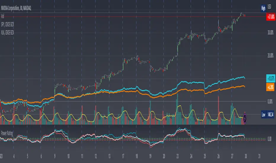
Stock Relative Strength Power IndexAs always, this is not financial advice and use at your own risk. Trading is risky and can cost you significant sums of money if you are not careful. Make sure you always have a proper entry and exit plan that includes defining your risk before you enter a trade.
This idea recently came out of some discussions I stumbled across in a trading group I am a part of regarding Relative Strength and Relative Weakness (shortened to RS and RW from here on out). The whole mechanism behind this trading system is to filter out underperforming securities relative to the current market direction to be in only the strongest or weakest stocks when the market is currently experiencing a bullish or bearish cycle. The idea behind this is there is no point in parking your money into a stock that is treading water or even going down if the market is making strong moves upwards. At that point, you are at worst losing money, and at best trading equal to the index/ETF, in which case the argument is why are you not just trading the index/ETF instead? RS or RW will filter out these sector laggards and allow you to position yourself into strong (or the strongest) stocks at any given time to help improve portfolio performance. Further, not only does it protect your position should the market shift against you briefly, it also often sees exceptional performance in the same cycle. For example, if $SPY makes a 5% move over the course of a month, a stock with RS/RW may make a 10% move, or more, allowing you to see increased profit potential.
RS/RW is based on the idea of performance, that is the raw percent change of a security over a given time period relative to a benchmark. This benchmark is often the S&P500 (ES/SPX/SPY and their derivatives). I have to stress that this is not beta, which measures the volatility of a stock over a given period (i.e. if $SPY moves $1, $NVDA will often move $1.74). This is a measurement of the market (i.e. $SPY) has moved 1% over the course of a day, $NVDA has moved 8% over the course of the day. This is very often used as a signal of institutional interest as apart from some very unique moments, retail traders cannot and will not provide enough market pressure to move a market outside of a stock's normal trading range, nor will they outperform the sector or market as a whole consistently over time without some big money to make them move. The problem with running strict performance analysis (i.e. % change from period T ago to period T + n at present) is that while it gives us a baseline of how much the stock has moved, it doesn't overall mean much. For instance, if a $100 stock has moved 5% today, but has been experiencing a period of increased volatility and it's Average True Range (ATR) (the amount a stock will move over X number of periods, on average) is $7, performance seems impressive but is actually generally fairly weak to what the stock has been doing recently. Conversely, if we take a second stock, this time worth $20, and it too has moved 5% in one day but has an ATR of only $0.25, that stock has made an exceptional move and we want to be part of that.
Here, I have created an indicator called the Stock Relative Strength Power Index. This takes the stock's rate of change (ROC) (the % move it has made over X number of periods), the stock's normalized ATR (the ATR represented as a percentage instead of a raw value), and compares these to one another to get the "Power Rating": a representation of the true strength of a stock over X number of periods. The indicator does two things. First, the raw ROC is divided by the stock's normalized ATR to assess whether the stock is moving outside of its normal range of variation or not. Second, since we are interested in trading only stocks with exceptional RS/RW to the market, I have also applied this same calculation to the S&P500 ($SPY) and the various SPDR sector indexes. These comparisons allow for a rapid and accurate assessment of the true strength of a stock at any given time on any given time frame. To cycle back above to our examples, the $100 stock has a Power Rating of only 0.71 (i.e. it is trading less than its current average), while our $20 stock has a Power Rating of 5. If we then compare these to both the market as a whole and the sector that the stock is a part of, we get a much clearer indication of the true buying or selling pressure imposed on the stock at any given time.
Use:
The indicator has 3 lines. The blue line is the security of interest, the red line is the market baseline (i.e. the sector ETF $SPY), and the white line is the sector index. I have given an example above on the semiconductor/tech stock $NVDA on a 30min timeframe. You can see that since the start of 2023, $NVDA has generally been strong to the market and its own sector since the blue line is greater than both the red and white lines over many days. This would have provided some nice day trading opportunities, or even some nice short term swing trades. The values themselves are generally meaningless outside of either the 1 or -1 value lines. All that matters is that the current ticker is surpassing both the market and the sector while being > 1.0 for a long trade or less than -1.0 for a short trade. However, I must stress this indicator gives no trade signals on its own, it is purely a confirmation indicator. An example of a trade would be if you had a trade signal given by either an indicator or by price action suggesting to buy some $NVDA for a trade to the upside, the Power Rating indicator would confirm this by showing if $NVDA was actually showing true strength by being both greater than 1 (the cutoff for it surpassing its ATR) and being above both the red and white lines. Further, you can see $NVDA has been stronger than the market when using the comparison function as well, but the has fluxed in and out of strength intraday when using the actual indicator vs. the static performance ratio chart (plotted as line graphs on the chart).
I have made it possible to change the colour of the plots and the line levels. The adjustment of the line levels gives the trader the flexibility to change their target breakout level (i.e. only trading stocks that have a Power Rating > 2, for example, meaning they are trading at least 2X their normal trading range). The third security comparison is flexible and can be used to compare to the sector ETF (initial intention) or it can be used to compare to other tickers within the same sector, for example. The trader should select the appropriate ETF for the given security of interest to avoid false confirmation if they want to use an ETF as their third input. The proper sector should be readily available on most online websites and accessible in a matter of seconds meaning that the delay is minimal, at worst. If a trader wishes to add additional functionality, such as a crypto trader using BTCUSD as the benchmark instead of $SPY, I encourage them to copy and paste this script and modify as needed since I have made this open source.
This indicator works on all timeframes. The lookback period can be changed, so a day trader who may use a 5min chart (and use a period of 12 to get the hourly Power Rating) will find this equally useful as someone who may be a core trader who wants to look at the performance over the course of years and may use a 60 period on a monthly chart.
Happy trading and I hope this helps!
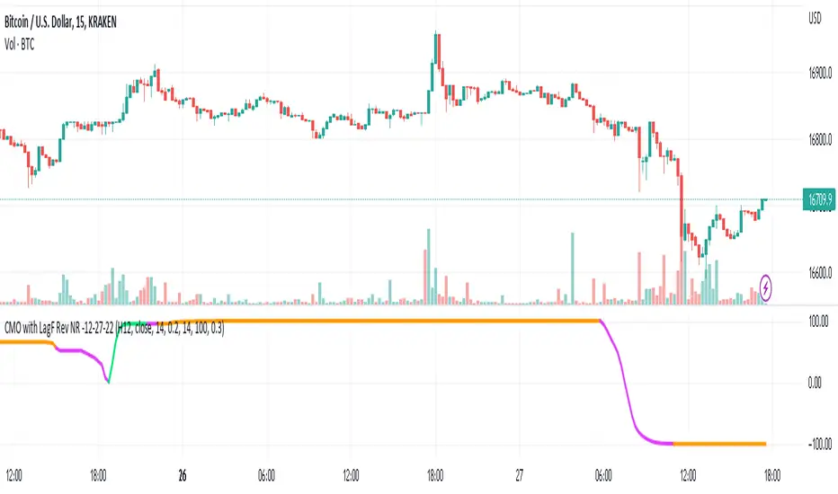
CMO with ATR and LagF Filtering - RevNR - 12-27-22Rev NR of the CMO ATR, with LagF Filtering - Released 12-27-22 by @Hockeydude84
This code takes Chande Momentum Oscillator (CMO), adds a coded ATR option and then filters the result through a Laguerre Filter (LagF) to reduce erroneous signals.
This code also has an option for self adjusting alpha on the Lag, via a lookback table and monitoring the price rate of change (ROC) in the lookback length.
Faster ROC will allow the LagF to move faster, slower price action will slow down LagF reaction. Pausing of signals is also present based on Rate of Change of the LagF Curve
Aggressive signals and Base signaling is allowed - aggressive bases signals on increase/decrease of previous LagF curve value point, Base is greater or less than 0
Original Code credits; Lost some of this due to time and multiple script manipulations, I believe the CMO origin code is from @TradingView House Code, and the LagF from @KıvançÖzbilgiç
Sharpe Ratio v4I'm publishing this indicator freely, because I'd like to get it reviewed by other people. This indicator was written whilst reading the book Systematic Trading by Robert Carver. In this book Carver describes trading rules that use a "dynamic" position size based on something like an evolving Sharpe Ratio . There are only a few other Sharpe indicators on TradingView, but they are either undocumented or use closed source code. You can use the following code as you wish for your own projects.
I'd like to let other people see this work, and let me know where they think this script is wrong, so that I can improve it.
Here's a basic rundown of Sharpe Ratio and its calculation.
SR is defined as: (excess) return minus the risk free rate divided by standard deviation of those returns. (This is where we're uncertain. Is the standard deviation of the returns, or just the closes?) But anyway the calculation itself is pretty simple:
SR = (r – b) ÷ s
Where r is the return of the asset over a certain period.
b is the interest rate of the risk-free asset.
s is the standard deviation of the returns over the same period.
For this indicator to "work" correctly, we're assuming the risk-free rate is 0. In fact, I did not include b at all in the indicator because it would make things too complicated, and go beyond the aim of this work.
To calculate the returns over a certain period, I'm using Rate of Change. Then calculating the standard deviation of those returns is pretty easy because we can use the same lookback period we used for ROC for the StDev calculation, thus:
averageReturn = ta.roc(close, lookbackLength)
stdev = ta.stdev(averageReturn, lookbackLength)
sharpe = (averageReturn / stdev)
Please leave a comment below if you believe this is incorrect. The chart shows a normal ROC indicator for comparison. I've also created a "bands" version of this indicator, which I'm planning to also release. The Keltner channel is just for comparing it with the StDev bands.

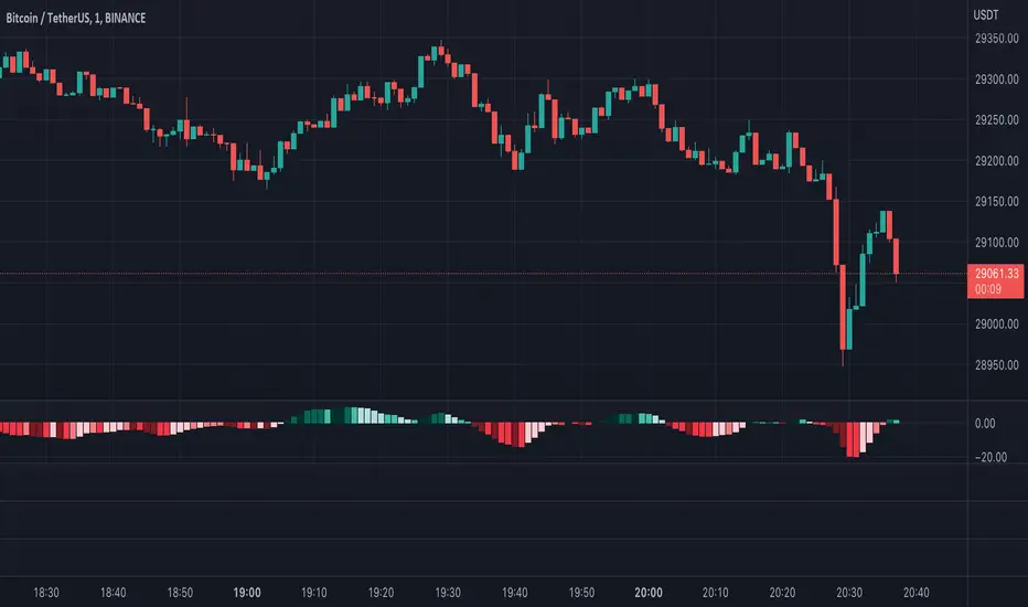
Moving Average Convergence Divergence with Rate of Change
Purpose - MACD is an awesome indicator. However, I felt I could improve the existing MACD indicator by also letting it visualize the rate of change (ROC) of the histogram (whether rate of change is increasing or decreasing - just like a derivative). By doing so, the indicator will better show the rate of change of the trend.
How It's Done - To the original MACD indicator, I have added a bit more conditional statements that automatically calculates the ROC in MACD histogram and visualizes through 8 different colors.
Interpretation - While the histogram is above 0, darker color indicates the stronger up trend, and lighter the color, weaker the up trend and potentially indicates the bears are overtaking, and vice versa for the case where the histogram is below 0.
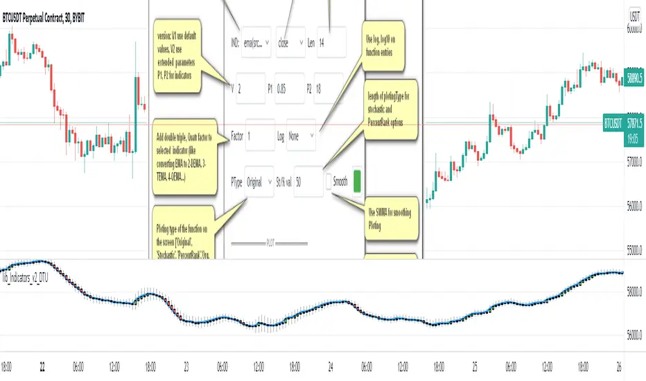
Indicator Functions with Factor and HeikinAshiHello all,
This indicator returns below selected indicators values with entered parameters.
Also you can add factorization, functions candles, function HeikinAshi and more to the plot.
VERSION:
Version 1: returns series only source and Length with already defined default values
Version 2: returns series with source, Length, p1 and p2 parameters according to the indicator definition (ex: )
PARAMETERS p1 p2
for defining multi arguments (See indicators list) indicator input value usable with verison=V2 selected.. ex: for alma( src , len ,offset=0.85,sigma=6), set source=source, len=length, p1=0.85 an p2=6
FACTOR:
Add double triple, Quadruple factors to selected indicator (like converting EMA to 2-DEMA, 3-TEMA, 4-QEMA...)
1-Original
2-Double
3-Triple
4-Quadruple
LOG
Log: Use log, log10 on function entries
PLOTTING:
PType: Plotting type of the function on the screen
Original :use original values
Org. Range (-1,1): usable for indicators between range -1 and 1
Stochastic: Convert indicator values by using stochastic calculation between -1 & 1. (use AT/% length to better view)
PercentRank: Convert indicator values by using Percent Rank calculation between -1 & 1. (use AT/% length to better view)
ST/%: length for plotting Type for stochastic and Percent Rank options
Smooth: Use SWMA for smoothing the function
DISPLAY TYPES
Plot Candles: Display the selected indicator as candle by implementing values
Plot Ind: Display result of indicator with selected source
HeikinAshi: Display Selected indicator candles with Heikin Ashi calculation
INDICATOR LIST:
hide = 'DONT DISPLAY', //Dont display & calculate the indicator. (For my framework usage)
alma = 'alma( src , len ,offset=0.85,sigma=6)', // Arnaud Legoux Moving Average
ama = 'ama( src , len ,fast=14,slow=100)', //Adjusted Moving Average
acdst = 'accdist()', // Accumulation/distribution index.
cma = 'cma( src , len )', //Corrective Moving average
dema = 'dema( src , len )', // Double EMA (Same as EMA with 2 factor)
ema = 'ema( src , len )', // Exponential Moving Average
gmma = 'gmma( src , len )', //Geometric Mean Moving Average
hghst = 'highest( src , len )', //Highest value for a given number of bars back.
hl2ma = 'hl2ma( src , len )', //higest lowest moving average
hma = 'hma( src , len )', // Hull Moving Average .
lgAdt = 'lagAdapt( src , len ,perclen=5,fperc=50)', //Ehler's Adaptive Laguerre filter
lgAdV = 'lagAdaptV( src , len ,perclen=5,fperc=50)', //Ehler's Adaptive Laguerre filter variation
lguer = 'laguerre( src , len )', //Ehler's Laguerre filter
lsrcp = 'lesrcp( src , len )', //lowest exponential esrcpanding moving line
lexp = 'lexp( src , len )', //lowest exponential expanding moving line
linrg = 'linreg( src , len ,loffset=1)', // Linear regression
lowst = 'lowest( src , len )', //Lovest value for a given number of bars back.
pcnl = 'percntl( src , len )', //percentile nearest rank. Calculates percentile using method of Nearest Rank.
pcnli = 'percntli( src , len )', //percentile linear interpolation. Calculates percentile using method of linear interpolation between the two nearest ranks.
rema = 'rema( src , len )', //Range EMA (REMA)
rma = 'rma( src , len )', //Moving average used in RSI . It is the exponentially weighted moving average with alpha = 1 / length.
sma = 'sma( src , len )', // Smoothed Moving Average
smma = 'smma( src , len )', // Smoothed Moving Average
supr2 = 'super2( src , len )', //Ehler's super smoother, 2 pole
supr3 = 'super3( src , len )', //Ehler's super smoother, 3 pole
strnd = 'supertrend( src , len ,period=3)', //Supertrend indicator
swma = 'swma( src , len )', //Sine-Weighted Moving Average
tema = 'tema( src , len )', // Triple EMA (Same as EMA with 3 factor)
tma = 'tma( src , len )', //Triangular Moving Average
vida = 'vida( src , len )', // Variable Index Dynamic Average
vwma = 'vwma( src , len )', // Volume Weigted Moving Average
wma = 'wma( src , len )', //Weigted Moving Average
angle = 'angle( src , len )', //angle of the series (Use its Input as another indicator output)
atr = 'atr( src , len )', // average true range . RMA of true range.
bbr = 'bbr( src , len ,mult=1)', // bollinger %%
bbw = 'bbw( src , len ,mult=2)', // Bollinger Bands Width . The Bollinger Band Width is the difference between the upper and the lower Bollinger Bands divided by the middle band.
cci = 'cci( src , len )', // commodity channel index
cctbb = 'cctbbo( src , len )', // CCT Bollinger Band Oscilator
chng = 'change( src , len )', //Difference between current value and previous, source - source.
cmo = 'cmo( src , len )', // Chande Momentum Oscillator . Calculates the difference between the sum of recent gains and the sum of recent losses and then divides the result by the sum of all price movement over the same period.
cog = 'cog( src , len )', //The cog (center of gravity ) is an indicator based on statistics and the Fibonacci golden ratio.
cpcrv = 'copcurve( src , len )', // Coppock Curve. was originally developed by Edwin "Sedge" Coppock (Barron's Magazine, October 1962).
corrl = 'correl( src , len )', // Correlation coefficient . Describes the degree to which two series tend to deviate from their ta. sma values.
count = 'count( src , len )', //green avg - red avg
dev = 'dev( src , len )', //ta.dev() Measure of difference between the series and it's ta. sma
fall = 'falling( src , len )', //ta.falling() Test if the `source` series is now falling for `length` bars long. (Use its Input as another indicator output)
kcr = 'kcr( src , len ,mult=2)', // Keltner Channels Range
kcw = 'kcw( src , len ,mult=2)', //ta.kcw(). Keltner Channels Width. The Keltner Channels Width is the difference between the upper and the lower Keltner Channels divided by the middle channel.
macd = 'macd( src , len )', // macd
mfi = 'mfi( src , len )', // Money Flow Index
nvi = 'nvi()', // Negative Volume Index
obv = 'obv()', // On Balance Volume
pvi = 'pvi()', // Positive Volume Index
pvt = 'pvt()', // Price Volume Trend
rise = 'rising( src , len )', //ta.rising() Test if the `source` series is now rising for `length` bars long. (Use its Input as another indicator output)
roc = 'roc( src , len )', // Rate of Change
rsi = 'rsi( src , len )', // Relative strength Index
smosc = 'smi_osc( src , len ,fast=5, slow=34)', //smi Oscillator
smsig = 'smi_sig( src , len ,fast=5, slow=34)', //smi Signal
stdev = 'stdev( src , len )', //Standart deviation
trix = 'trix( src , len )' , //the rate of change of a triple exponentially smoothed moving average .
tsi = 'tsi( src , len )', //True Strength Index
vari = 'variance( src , len )', //ta.variance(). Variance is the expectation of the squared deviation of a series from its mean (ta. sma ), and it informally measures how far a set of numbers are spread out from their mean.
wilpc = 'willprc( src , len )', // Williams %R
wad = 'wad()', // Williams Accumulation/Distribution .
wvad = 'wvad()' //Williams Variable Accumulation/Distribution
I will update the indicator list when I will update the library
Thanks to tradingview, @RodrigoKazuma for their open source indicators

lib_Indicators_v2_DTULibrary "lib_Indicators_v2_DTU"
This library functions returns included Moving averages, indicators with factorization, functions candles, function heikinashi and more.
Created it to feed as backend of my indicator/strategy "Indicators & Combinations Framework Advanced v2 " that will be released ASAP.
This is replacement of my previous indicator (lib_indicators_DT)
I will add an indicator example which will use this indicator named as "lib_indicators_v2_DTU example" to help the usage of this library
Additionally library will be updated with more indicators in the future
NOTES:
Indicator functions returns only one series :-(
plotcandle function returns candle series
INDICATOR LIST:
hide = 'DONT DISPLAY', //Dont display & calculate the indicator. (For my framework usage)
alma = 'alma(src,len,offset=0.85,sigma=6)', //Arnaud Legoux Moving Average
ama = 'ama(src,len,fast=14,slow=100)', //Adjusted Moving Average
acdst = 'accdist()', //Accumulation/distribution index.
cma = 'cma(src,len)', //Corrective Moving average
dema = 'dema(src,len)', //Double EMA (Same as EMA with 2 factor)
ema = 'ema(src,len)', //Exponential Moving Average
gmma = 'gmma(src,len)', //Geometric Mean Moving Average
hghst = 'highest(src,len)', //Highest value for a given number of bars back.
hl2ma = 'hl2ma(src,len)', //higest lowest moving average
hma = 'hma(src,len)', //Hull Moving Average.
lgAdt = 'lagAdapt(src,len,perclen=5,fperc=50)', //Ehler's Adaptive Laguerre filter
lgAdV = 'lagAdaptV(src,len,perclen=5,fperc=50)', //Ehler's Adaptive Laguerre filter variation
lguer = 'laguerre(src,len)', //Ehler's Laguerre filter
lsrcp = 'lesrcp(src,len)', //lowest exponential esrcpanding moving line
lexp = 'lexp(src,len)', //lowest exponential expanding moving line
linrg = 'linreg(src,len,loffset=1)', //Linear regression
lowst = 'lowest(src,len)', //Lovest value for a given number of bars back.
pcnl = 'percntl(src,len)', //percentile nearest rank. Calculates percentile using method of Nearest Rank.
pcnli = 'percntli(src,len)', //percentile linear interpolation. Calculates percentile using method of linear interpolation between the two nearest ranks.
rema = 'rema(src,len)', //Range EMA (REMA)
rma = 'rma(src,len)', //Moving average used in RSI. It is the exponentially weighted moving average with alpha = 1 / length.
sma = 'sma(src,len)', //Smoothed Moving Average
smma = 'smma(src,len)', //Smoothed Moving Average
supr2 = 'super2(src,len)', //Ehler's super smoother, 2 pole
supr3 = 'super3(src,len)', //Ehler's super smoother, 3 pole
strnd = 'supertrend(src,len,period=3)', //Supertrend indicator
swma = 'swma(src,len)', //Sine-Weighted Moving Average
tema = 'tema(src,len)', //Triple EMA (Same as EMA with 3 factor)
tma = 'tma(src,len)', //Triangular Moving Average
vida = 'vida(src,len)', //Variable Index Dynamic Average
vwma = 'vwma(src,len)', //Volume Weigted Moving Average
wma = 'wma(src,len)', //Weigted Moving Average
angle = 'angle(src,len)', //angle of the series (Use its Input as another indicator output)
atr = 'atr(src,len)', //average true range. RMA of true range.
bbr = 'bbr(src,len,mult=1)', //bollinger %%
bbw = 'bbw(src,len,mult=2)', //Bollinger Bands Width. The Bollinger Band Width is the difference between the upper and the lower Bollinger Bands divided by the middle band.
cci = 'cci(src,len)', //commodity channel index
cctbb = 'cctbbo(src,len)', //CCT Bollinger Band Oscilator
chng = 'change(src,len)', //Difference between current value and previous, source - source .
cmo = 'cmo(src,len)', //Chande Momentum Oscillator. Calculates the difference between the sum of recent gains and the sum of recent losses and then divides the result by the sum of all price movement over the same period.
cog = 'cog(src,len)', //The cog (center of gravity) is an indicator based on statistics and the Fibonacci golden ratio.
cpcrv = 'copcurve(src,len)', //Coppock Curve. was originally developed by Edwin "Sedge" Coppock (Barron's Magazine, October 1962).
corrl = 'correl(src,len)', //Correlation coefficient. Describes the degree to which two series tend to deviate from their ta.sma values.
count = 'count(src,len)', //green avg - red avg
dev = 'dev(src,len)', //ta.dev() Measure of difference between the series and it's ta.sma
fall = 'falling(src,len)', //ta.falling() Test if the `source` series is now falling for `length` bars long. (Use its Input as another indicator output)
kcr = 'kcr(src,len,mult=2)', //Keltner Channels Range
kcw = 'kcw(src,len,mult=2)', //ta.kcw(). Keltner Channels Width. The Keltner Channels Width is the difference between the upper and the lower Keltner Channels divided by the middle channel.
macd = 'macd(src,len)', //macd
mfi = 'mfi(src,len)', //Money Flow Index
nvi = 'nvi()', //Negative Volume Index
obv = 'obv()', //On Balance Volume
pvi = 'pvi()', //Positive Volume Index
pvt = 'pvt()', //Price Volume Trend
rise = 'rising(src,len)', //ta.rising() Test if the `source` series is now rising for `length` bars long. (Use its Input as another indicator output)
roc = 'roc(src,len)', //Rate of Change
rsi = 'rsi(src,len)', //Relative strength Index
smosc = 'smi_osc(src,len,fast=5, slow=34)', //smi Oscillator
smsig = 'smi_sig(src,len,fast=5, slow=34)', //smi Signal
stdev = 'stdev(src,len)', //Standart deviation
trix = 'trix(src,len)' , //the rate of change of a triple exponentially smoothed moving average.
tsi = 'tsi(src,len)', //True Strength Index
vari = 'variance(src,len)', //ta.variance(). Variance is the expectation of the squared deviation of a series from its mean (ta.sma), and it informally measures how far a set of numbers are spread out from their mean.
wilpc = 'willprc(src,len)', //Williams %R
wad = 'wad()', //Williams Accumulation/Distribution.
wvad = 'wvad()' //Williams Variable Accumulation/Distribution.
}
f_func(string, float, simple, float, float, float, simple) f_func Return selected indicator value with different parameters. New version. Use extra parameters for available indicators
Parameters:
string : FuncType_ indicator from the indicator list
float : src_ close, open, high, low,hl2, hlc3, ohlc4 or any
simple : int length_ indicator length
float : p1 extra parameter-1. active on Version 2 for defining multi arguments indicator input value. ex: lagAdapt(src_, length_,LAPercLen_=p1,FPerc_=p2)
float : p2 extra parameter-2. active on Version 2 for defining multi arguments indicator input value. ex: lagAdapt(src_, length_,LAPercLen_=p1,FPerc_=p2)
float : p3 extra parameter-3. active on Version 2 for defining multi arguments indicator input value. ex: lagAdapt(src_, length_,LAPercLen_=p1,FPerc_=p2)
simple : int version_ indicator version for backward compatibility. V1:dont use extra parameters p1,p2,p3 and use default values. V2: use extra parameters for available indicators
Returns: float Return calculated indicator value
fn_heikin(float, float, float, float) fn_heikin Return given src data (open, high,low,close) as heikin ashi candle values
Parameters:
float : o_ open value
float : h_ high value
float : l_ low value
float : c_ close value
Returns: float heikin ashi open, high,low,close vlues that will be used with plotcandle
fn_plotFunction(float, string, simple, bool) fn_plotFunction Return input src data with different plotting options
Parameters:
float : src_ indicator src_data or any other series.....
string : plotingType Ploting type of the function on the screen
simple : int stochlen_ length for plotingType for stochastic and PercentRank options
bool : plotSWMA Use SWMA for smoothing Ploting
Returns: float
fn_funcPlotV2(string, float, simple, float, float, float, simple, string, simple, bool, bool) fn_funcPlotV2 Return selected indicator value with different parameters. New version. Use extra parameters fora available indicators
Parameters:
string : FuncType_ indicator from the indicator list
float : src_data_ close, open, high, low,hl2, hlc3, ohlc4 or any
simple : int length_ indicator length
float : p1 extra parameter-1. active on Version 2 for defining multi arguments indicator input value. ex: lagAdapt(src_, length_,LAPercLen_=p1,FPerc_=p2)
float : p2 extra parameter-2. active on Version 2 for defining multi arguments indicator input value. ex: lagAdapt(src_, length_,LAPercLen_=p1,FPerc_=p2)
float : p3 extra parameter-3. active on Version 2 for defining multi arguments indicator input value. ex: lagAdapt(src_, length_,LAPercLen_=p1,FPerc_=p2)
simple : int version_ indicator version for backward compatibility. V1:dont use extra parameters p1,p2,p3 and use default values. V2: use extra parameters for available indicators
string : plotingType Ploting type of the function on the screen
simple : int stochlen_ length for plotingType for stochastic and PercentRank options
bool : plotSWMA Use SWMA for smoothing Ploting
bool : log_ Use log on function entries
Returns: float Return calculated indicator value
fn_factor(string, float, simple, float, float, float, simple, simple, string, simple, bool, bool) fn_factor Return selected indicator's factorization with given arguments
Parameters:
string : FuncType_ indicator from the indicator list
float : src_data_ close, open, high, low,hl2, hlc3, ohlc4 or any
simple : int length_ indicator length
float : p1 parameter-1. active on Version 2 for defining multi arguments indicator input value. ex: lagAdapt(src_, length_,LAPercLen_=p1,FPerc_=p2)
float : p2 parameter-2. active on Version 2 for defining multi arguments indicator input value. ex: lagAdapt(src_, length_,LAPercLen_=p1,FPerc_=p2)
float : p3 parameter-3. active on Version 2 for defining multi arguments indicator input value. ex: lagAdapt(src_, length_,LAPercLen_=p1,FPerc_=p2)
simple : int version_ indicator version for backward compatibility. V1:dont use extra parameters p1,p2,p3 and use default values. V2: use extra parameters for available indicators
simple : int fact_ Add double triple, Quatr factor to selected indicator (like converting EMA to 2-DEMA, 3-TEMA, 4-QEMA...)
string : plotingType Ploting type of the function on the screen
simple : int stochlen_ length for plotingType for stochastic and PercentRank options
bool : plotSWMA Use SWMA for smoothing Ploting
bool : log_ Use log on function entries
Returns: float Return result of the function
fn_plotCandles(string, simple, float, float, float, simple, string, simple, bool, bool, bool) fn_plotCandles Return selected indicator's candle values with different parameters also heikinashi is available
Parameters:
string : FuncType_ indicator from the indicator list
simple : int length_ indicator length
float : p1 parameter-1. active on Version 2 for defining multi arguments indicator input value. ex: lagAdapt(src_, length_,LAPercLen_=p1,FPerc_=p2)
float : p2 parameter-2. active on Version 2 for defining multi arguments indicator input value. ex: lagAdapt(src_, length_,LAPercLen_=p1,FPerc_=p2)
float : p3 parameter-3. active on Version 2 for defining multi arguments indicator input value. ex: lagAdapt(src_, length_,LAPercLen_=p1,FPerc_=p2)
simple : int version_ indicator version for backward compatibility. V1:dont use extra parameters p1,p2,p3 and use default values. V2: use extra parameters for available indicators
string : plotingType Ploting type of the function on the screen
simple : int stochlen_ length for plotingType for stochastic and PercentRank options
bool : plotSWMA Use SWMA for smoothing Ploting
bool : log_ Use log on function entries
bool : plotheikin_ Use Heikin Ashi on Plot
Returns: float
+ Rate of ChangeNOTE!* If you were using my previous + Rate of Change (and OBV) indicator, I will not be updating that. OBV was moved to my + Breadth & Volume indicator.
This indicator here is basically and updated version of the old indicator, without OBV.
The Rate of Change, or RoC, is a momentum indicator that measures the percentage change in price between the current period and the price n periods ago.
It oscillates above and below a zeroline, basically showing positive or negative momentum.
I applied the OBV's calculation to it, but without the inclusion of volume (also added a lookback period) to see what would happen. I rather liked the result.
I call this the "Cumulative Rate of Change." I only recently realized that this is actually just the OBV without volume, however the OBV does not have a lookback period, and this indicator does.
Doing some more fiddling, I realized that removing both the signum and the volume from the calculation gets you basically a price chart, but calculated as the change in price over n periods. I'm leaving this in because maybe someone discovers they really like having a line chart with moving averages or some other indicator on it to leave their main chart indicator free (giving a more clear look at price action). Can't hurt, right?
Default lookback is set to 1, but play with longer settings (especially if using the traditional RoC, which is by default in TV set to 10, and is nigh on useless at 1--I like 13).
Default source is set to each candle close, but give ohlc4 a look. It smooths out the indicator a bit, and because it's an average of the open, high, low, and close it should give a better idea of what price in general is doing.
Moving averages, Bollinger Bands, Donchian Channels, candle coloring and alerts are my usual additions.
Below are some comparison images of the different indicators wrapped up in here.
Comparison of Cumulative Rate of Change with two different sources. Lookback set to 1.
Cumulative Rate of Change as a price chart, essentially.
And, lastly, the traditional Rate of Change indicator.

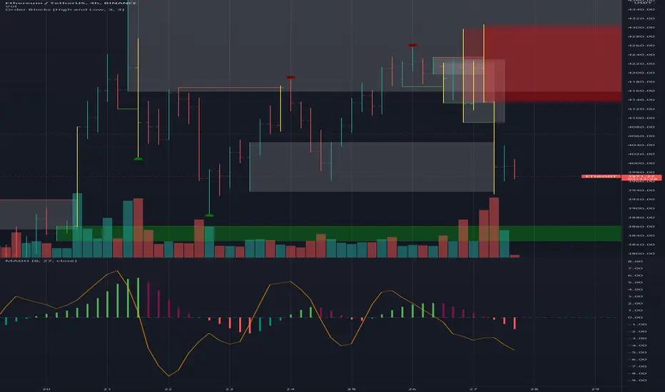
MAD indicator Enchanced (MADH, inspired by J.Ehlers)This oscillator was inspired by the recent J. Ehler's article (Stocks & Commodities V. 39:11 (24–26): The MAD Indicator, Enhanced by John F. Ehlers). Basically, it shows the difference between two move averages, an "enhancement" made by the author in the last version comes down to replacement SMA to a weighted average that uses Hann windowing. I took the liberty to add colors, ROC line (well, you know, no shorts when ROC's negative and no long's when positive, etc), and optional usage of PVT (price-volume trend) as the source (instead of just price).
taLibrary "ta"
█ OVERVIEW
This library holds technical analysis functions calculating values for which no Pine built-in exists.
Look first. Then leap.
█ FUNCTIONS
cagr(entryTime, entryPrice, exitTime, exitPrice)
It calculates the "Compound Annual Growth Rate" between two points in time. The CAGR is a notional, annualized growth rate that assumes all profits are reinvested. It only takes into account the prices of the two end points — not drawdowns, so it does not calculate risk. It can be used as a yardstick to compare the performance of two instruments. Because it annualizes values, the function requires a minimum of one day between the two end points (annualizing returns over smaller periods of times doesn't produce very meaningful figures).
Parameters:
entryTime : The starting timestamp.
entryPrice : The starting point's price.
exitTime : The ending timestamp.
exitPrice : The ending point's price.
Returns: CAGR in % (50 is 50%). Returns `na` if there is not >=1D between `entryTime` and `exitTime`, or until the two time points have not been reached by the script.
█ v2, Mar. 8, 2022
Added functions `allTimeHigh()` and `allTimeLow()` to find the highest or lowest value of a source from the first historical bar to the current bar. These functions will not look ahead; they will only return new highs/lows on the bar where they occur.
allTimeHigh(src)
Tracks the highest value of `src` from the first historical bar to the current bar.
Parameters:
src : (series int/float) Series to track. Optional. The default is `high`.
Returns: (float) The highest value tracked.
allTimeLow(src)
Tracks the lowest value of `src` from the first historical bar to the current bar.
Parameters:
src : (series int/float) Series to track. Optional. The default is `low`.
Returns: (float) The lowest value tracked.
█ v3, Sept. 27, 2022
This version includes the following new functions:
aroon(length)
Calculates the values of the Aroon indicator.
Parameters:
length (simple int) : (simple int) Number of bars (length).
Returns: ( [float, float ]) A tuple of the Aroon-Up and Aroon-Down values.
coppock(source, longLength, shortLength, smoothLength)
Calculates the value of the Coppock Curve indicator.
Parameters:
source (float) : (series int/float) Series of values to process.
longLength (simple int) : (simple int) Number of bars for the fast ROC value (length).
shortLength (simple int) : (simple int) Number of bars for the slow ROC value (length).
smoothLength (simple int) : (simple int) Number of bars for the weigted moving average value (length).
Returns: (float) The oscillator value.
dema(source, length)
Calculates the value of the Double Exponential Moving Average (DEMA).
Parameters:
source (float) : (series int/float) Series of values to process.
length (simple int) : (simple int) Length for the smoothing parameter calculation.
Returns: (float) The double exponentially weighted moving average of the `source`.
dema2(src, length)
An alternate Double Exponential Moving Average (Dema) function to `dema()`, which allows a "series float" length argument.
Parameters:
src : (series int/float) Series of values to process.
length : (series int/float) Length for the smoothing parameter calculation.
Returns: (float) The double exponentially weighted moving average of the `src`.
dm(length)
Calculates the value of the "Demarker" indicator.
Parameters:
length (simple int) : (simple int) Number of bars (length).
Returns: (float) The oscillator value.
donchian(length)
Calculates the values of a Donchian Channel using `high` and `low` over a given `length`.
Parameters:
length (int) : (series int) Number of bars (length).
Returns: ( [float, float, float ]) A tuple containing the channel high, low, and median, respectively.
ema2(src, length)
An alternate ema function to the `ta.ema()` built-in, which allows a "series float" length argument.
Parameters:
src : (series int/float) Series of values to process.
length : (series int/float) Number of bars (length).
Returns: (float) The exponentially weighted moving average of the `src`.
eom(length, div)
Calculates the value of the Ease of Movement indicator.
Parameters:
length (simple int) : (simple int) Number of bars (length).
div (simple int) : (simple int) Divisor used for normalzing values. Optional. The default is 10000.
Returns: (float) The oscillator value.
frama(source, length)
The Fractal Adaptive Moving Average (FRAMA), developed by John Ehlers, is an adaptive moving average that dynamically adjusts its lookback period based on fractal geometry.
Parameters:
source (float) : (series int/float) Series of values to process.
length (int) : (series int) Number of bars (length).
Returns: (float) The fractal adaptive moving average of the `source`.
ft(source, length)
Calculates the value of the Fisher Transform indicator.
Parameters:
source (float) : (series int/float) Series of values to process.
length (simple int) : (simple int) Number of bars (length).
Returns: (float) The oscillator value.
ht(source)
Calculates the value of the Hilbert Transform indicator.
Parameters:
source (float) : (series int/float) Series of values to process.
Returns: (float) The oscillator value.
ichimoku(conLength, baseLength, senkouLength)
Calculates values of the Ichimoku Cloud indicator, including tenkan, kijun, senkouSpan1, senkouSpan2, and chikou. NOTE: offsets forward or backward can be done using the `offset` argument in `plot()`.
Parameters:
conLength (int) : (series int) Length for the Conversion Line (Tenkan). The default is 9 periods, which returns the mid-point of the 9 period Donchian Channel.
baseLength (int) : (series int) Length for the Base Line (Kijun-sen). The default is 26 periods, which returns the mid-point of the 26 period Donchian Channel.
senkouLength (int) : (series int) Length for the Senkou Span 2 (Leading Span B). The default is 52 periods, which returns the mid-point of the 52 period Donchian Channel.
Returns: ( [float, float, float, float, float ]) A tuple of the Tenkan, Kijun, Senkou Span 1, Senkou Span 2, and Chikou Span values. NOTE: by default, the senkouSpan1 and senkouSpan2 should be plotted 26 periods in the future, and the Chikou Span plotted 26 days in the past.
ift(source)
Calculates the value of the Inverse Fisher Transform indicator.
Parameters:
source (float) : (series int/float) Series of values to process.
Returns: (float) The oscillator value.
kvo(fastLen, slowLen, trigLen)
Calculates the values of the Klinger Volume Oscillator.
Parameters:
fastLen (simple int) : (simple int) Length for the fast moving average smoothing parameter calculation.
slowLen (simple int) : (simple int) Length for the slow moving average smoothing parameter calculation.
trigLen (simple int) : (simple int) Length for the trigger moving average smoothing parameter calculation.
Returns: ( [float, float ]) A tuple of the KVO value, and the trigger value.
pzo(length)
Calculates the value of the Price Zone Oscillator.
Parameters:
length (simple int) : (simple int) Length for the smoothing parameter calculation.
Returns: (float) The oscillator value.
rms(source, length)
Calculates the Root Mean Square of the `source` over the `length`.
Parameters:
source (float) : (series int/float) Series of values to process.
length (int) : (series int) Number of bars (length).
Returns: (float) The RMS value.
rwi(length)
Calculates the values of the Random Walk Index.
Parameters:
length (simple int) : (simple int) Lookback and ATR smoothing parameter length.
Returns: ( [float, float ]) A tuple of the `rwiHigh` and `rwiLow` values.
stc(source, fast, slow, cycle, d1, d2)
Calculates the value of the Schaff Trend Cycle indicator.
Parameters:
source (float) : (series int/float) Series of values to process.
fast (simple int) : (simple int) Length for the MACD fast smoothing parameter calculation.
slow (simple int) : (simple int) Length for the MACD slow smoothing parameter calculation.
cycle (simple int) : (simple int) Number of bars for the Stochastic values (length).
d1 (simple int) : (simple int) Length for the initial %D smoothing parameter calculation.
d2 (simple int) : (simple int) Length for the final %D smoothing parameter calculation.
Returns: (float) The oscillator value.
stochFull(periodK, smoothK, periodD)
Calculates the %K and %D values of the Full Stochastic indicator.
Parameters:
periodK (simple int) : (simple int) Number of bars for Stochastic calculation. (length).
smoothK (simple int) : (simple int) Number of bars for smoothing of the %K value (length).
periodD (simple int) : (simple int) Number of bars for smoothing of the %D value (length).
Returns: ( [float, float ]) A tuple of the slow %K and the %D moving average values.
stochRsi(lengthRsi, periodK, smoothK, periodD, source)
Calculates the %K and %D values of the Stochastic RSI indicator.
Parameters:
lengthRsi (simple int) : (simple int) Length for the RSI smoothing parameter calculation.
periodK (simple int) : (simple int) Number of bars for Stochastic calculation. (length).
smoothK (simple int) : (simple int) Number of bars for smoothing of the %K value (length).
periodD (simple int) : (simple int) Number of bars for smoothing of the %D value (length).
source (float) : (series int/float) Series of values to process. Optional. The default is `close`.
Returns: ( [float, float ]) A tuple of the slow %K and the %D moving average values.
supertrend(factor, atrLength, wicks)
Calculates the values of the SuperTrend indicator with the ability to take candle wicks into account, rather than only the closing price.
Parameters:
factor (float) : (series int/float) Multiplier for the ATR value.
atrLength (simple int) : (simple int) Length for the ATR smoothing parameter calculation.
wicks (simple bool) : (simple bool) Condition to determine whether to take candle wicks into account when reversing trend, or to use the close price. Optional. Default is false.
Returns: ( [float, int ]) A tuple of the superTrend value and trend direction.
szo(source, length)
Calculates the value of the Sentiment Zone Oscillator.
Parameters:
source (float) : (series int/float) Series of values to process.
length (simple int) : (simple int) Length for the smoothing parameter calculation.
Returns: (float) The oscillator value.
t3(source, length, vf)
Calculates the value of the Tilson Moving Average (T3).
Parameters:
source (float) : (series int/float) Series of values to process.
length (simple int) : (simple int) Length for the smoothing parameter calculation.
vf (simple float) : (simple float) Volume factor. Affects the responsiveness.
Returns: (float) The Tilson moving average of the `source`.
t3Alt(source, length, vf)
An alternate Tilson Moving Average (T3) function to `t3()`, which allows a "series float" `length` argument.
Parameters:
source (float) : (series int/float) Series of values to process.
length (float) : (series int/float) Length for the smoothing parameter calculation.
vf (simple float) : (simple float) Volume factor. Affects the responsiveness.
Returns: (float) The Tilson moving average of the `source`.
tema(source, length)
Calculates the value of the Triple Exponential Moving Average (TEMA).
Parameters:
source (float) : (series int/float) Series of values to process.
length (simple int) : (simple int) Length for the smoothing parameter calculation.
Returns: (float) The triple exponentially weighted moving average of the `source`.
tema2(source, length)
An alternate Triple Exponential Moving Average (TEMA) function to `tema()`, which allows a "series float" `length` argument.
Parameters:
source (float) : (series int/float) Series of values to process.
length (float) : (series int/float) Length for the smoothing parameter calculation.
Returns: (float) The triple exponentially weighted moving average of the `source`.
trima(source, length)
Calculates the value of the Triangular Moving Average (TRIMA).
Parameters:
source (float) : (series int/float) Series of values to process.
length (int) : (series int) Number of bars (length).
Returns: (float) The triangular moving average of the `source`.
trima2(src, length)
An alternate Triangular Moving Average (TRIMA) function to `trima()`, which allows a "series int" length argument.
Parameters:
src : (series int/float) Series of values to process.
length : (series int) Number of bars (length).
Returns: (float) The triangular moving average of the `src`.
trix(source, length, signalLength, exponential)
Calculates the values of the TRIX indicator.
Parameters:
source (float) : (series int/float) Series of values to process.
length (simple int) : (simple int) Length for the smoothing parameter calculation.
signalLength (simple int) : (simple int) Length for smoothing the signal line.
exponential (simple bool) : (simple bool) Condition to determine whether exponential or simple smoothing is used. Optional. The default is `true` (exponential smoothing).
Returns: ( [float, float, float ]) A tuple of the TRIX value, the signal value, and the histogram.
uo(fastLen, midLen, slowLen)
Calculates the value of the Ultimate Oscillator.
Parameters:
fastLen (simple int) : (series int) Number of bars for the fast smoothing average (length).
midLen (simple int) : (series int) Number of bars for the middle smoothing average (length).
slowLen (simple int) : (series int) Number of bars for the slow smoothing average (length).
Returns: (float) The oscillator value.
vhf(source, length)
Calculates the value of the Vertical Horizontal Filter.
Parameters:
source (float) : (series int/float) Series of values to process.
length (simple int) : (simple int) Number of bars (length).
Returns: (float) The oscillator value.
vi(length)
Calculates the values of the Vortex Indicator.
Parameters:
length (simple int) : (simple int) Number of bars (length).
Returns: ( [float, float ]) A tuple of the viPlus and viMinus values.
vzo(length)
Calculates the value of the Volume Zone Oscillator.
Parameters:
length (simple int) : (simple int) Length for the smoothing parameter calculation.
Returns: (float) The oscillator value.
williamsFractal(period)
Detects Williams Fractals.
Parameters:
period (int) : (series int) Number of bars (length).
Returns: ( [bool, bool ]) A tuple of an up fractal and down fractal. Variables are true when detected.
wpo(length)
Calculates the value of the Wave Period Oscillator.
Parameters:
length (simple int) : (simple int) Length for the smoothing parameter calculation.
Returns: (float) The oscillator value.
█ v7, Nov. 2, 2023
This version includes the following new and updated functions:
atr2(length)
An alternate ATR function to the `ta.atr()` built-in, which allows a "series float" `length` argument.
Parameters:
length (float) : (series int/float) Length for the smoothing parameter calculation.
Returns: (float) The ATR value.
changePercent(newValue, oldValue)
Calculates the percentage difference between two distinct values.
Parameters:
newValue (float) : (series int/float) The current value.
oldValue (float) : (series int/float) The previous value.
Returns: (float) The percentage change from the `oldValue` to the `newValue`.
donchian(length)
Calculates the values of a Donchian Channel using `high` and `low` over a given `length`.
Parameters:
length (int) : (series int) Number of bars (length).
Returns: ( [float, float, float ]) A tuple containing the channel high, low, and median, respectively.
highestSince(cond, source)
Tracks the highest value of a series since the last occurrence of a condition.
Parameters:
cond (bool) : (series bool) A condition which, when `true`, resets the tracking of the highest `source`.
source (float) : (series int/float) Series of values to process. Optional. The default is `high`.
Returns: (float) The highest `source` value since the last time the `cond` was `true`.
lowestSince(cond, source)
Tracks the lowest value of a series since the last occurrence of a condition.
Parameters:
cond (bool) : (series bool) A condition which, when `true`, resets the tracking of the lowest `source`.
source (float) : (series int/float) Series of values to process. Optional. The default is `low`.
Returns: (float) The lowest `source` value since the last time the `cond` was `true`.
relativeVolume(length, anchorTimeframe, isCumulative, adjustRealtime)
Calculates the volume since the last change in the time value from the `anchorTimeframe`, the historical average volume using bars from past periods that have the same relative time offset as the current bar from the start of its period, and the ratio of these volumes. The volume values are cumulative by default, but can be adjusted to non-accumulated with the `isCumulative` parameter.
Parameters:
length (simple int) : (simple int) The number of periods to use for the historical average calculation.
anchorTimeframe (simple string) : (simple string) The anchor timeframe used in the calculation. Optional. Default is "D".
isCumulative (simple bool) : (simple bool) If `true`, the volume values will be accumulated since the start of the last `anchorTimeframe`. If `false`, values will be used without accumulation. Optional. The default is `true`.
adjustRealtime (simple bool) : (simple bool) If `true`, estimates the cumulative value on unclosed bars based on the data since the last `anchor` condition. Optional. The default is `false`.
Returns: ( [float, float, float ]) A tuple of three float values. The first element is the current volume. The second is the average of volumes at equivalent time offsets from past anchors over the specified number of periods. The third is the ratio of the current volume to the historical average volume.
rma2(source, length)
An alternate RMA function to the `ta.rma()` built-in, which allows a "series float" `length` argument.
Parameters:
source (float) : (series int/float) Series of values to process.
length (float) : (series int/float) Length for the smoothing parameter calculation.
Returns: (float) The rolling moving average of the `source`.
supertrend2(factor, atrLength, wicks)
An alternate SuperTrend function to `supertrend()`, which allows a "series float" `atrLength` argument.
Parameters:
factor (float) : (series int/float) Multiplier for the ATR value.
atrLength (float) : (series int/float) Length for the ATR smoothing parameter calculation.
wicks (simple bool) : (simple bool) Condition to determine whether to take candle wicks into account when reversing trend, or to use the close price. Optional. Default is `false`.
Returns: ( [float, int ]) A tuple of the superTrend value and trend direction.
vStop(source, atrLength, atrFactor)
Calculates an ATR-based stop value that trails behind the `source`. Can serve as a possible stop-loss guide and trend identifier.
Parameters:
source (float) : (series int/float) Series of values that the stop trails behind.
atrLength (simple int) : (simple int) Length for the ATR smoothing parameter calculation.
atrFactor (float) : (series int/float) The multiplier of the ATR value. Affects the maximum distance between the stop and the `source` value. A value of 1 means the maximum distance is 100% of the ATR value. Optional. The default is 1.
Returns: ( [float, bool ]) A tuple of the volatility stop value and the trend direction as a "bool".
vStop2(source, atrLength, atrFactor)
An alternate Volatility Stop function to `vStop()`, which allows a "series float" `atrLength` argument.
Parameters:
source (float) : (series int/float) Series of values that the stop trails behind.
atrLength (float) : (series int/float) Length for the ATR smoothing parameter calculation.
atrFactor (float) : (series int/float) The multiplier of the ATR value. Affects the maximum distance between the stop and the `source` value. A value of 1 means the maximum distance is 100% of the ATR value. Optional. The default is 1.
Returns: ( [float, bool ]) A tuple of the volatility stop value and the trend direction as a "bool".
Removed Functions:
allTimeHigh(src)
Tracks the highest value of `src` from the first historical bar to the current bar.
allTimeLow(src)
Tracks the lowest value of `src` from the first historical bar to the current bar.
trima2(src, length)
An alternate Triangular Moving Average (TRIMA) function to `trima()`, which allows a
"series int" length argument.

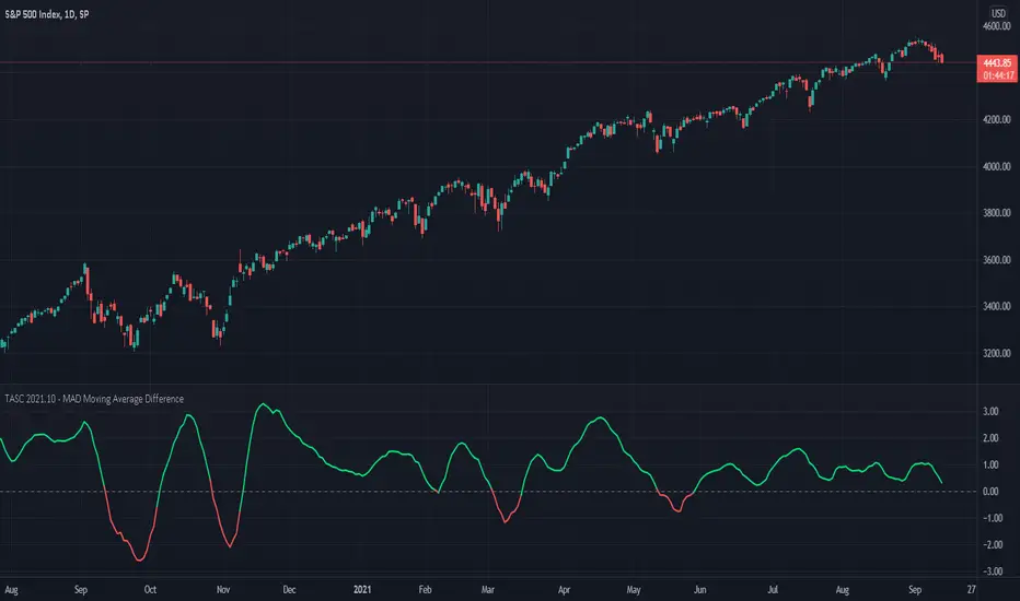
TASC 2021.10 - MAD Moving Average DifferencePresented here is code for the "Moving Average Difference" indicator originally conceived by John Ehlers, also referred to as MAD. This is one of TradingView's first code releases published in the October 2021 issue of Trader's Tips by Technical Analysis of Stocks & Commodities (TASC) magazine.
This indicator has a companion indicator that is discussed in the article entitled Cycle/Trend Analytics And The MAD Indicator , authored by John Ehlers. He's providing an innovative double dose of indicator code for the month of October 2021.
John Ehlers generally describes it as a "thinking man's" MACD . MAD has similar, yet distinct, intended operation. For those of you familiar with the MACD indicator operation, you will find MACD adjustments having defaults of 12 and 26, while MAD has comparable adjustments with defaults of 8 and 23. These are intended for adjustment, same as any other oscillator.
The MAD indicator can be basically described as two simple moving averages applied within a "rate of change" (ROC) calculation.
Further Related Information
• SMA
• ROC
Join TradingView!
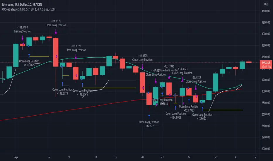
Rate of Change StrategyThis strategy calculates the rate of change over time to determine buy/sell points. This strategy is best run with 1 hour candles .
Configurable values:
SMA Fast (days)
SMA Slow (days)
SMA Reference (days)
ROC Low (%)
ROC High (%)
Order Stake (%)
Look back Candles
FIR Hann Window Indicator (Ehlers)From Ehlers' Windowing article:
"A still-smoother weighting function that is easy to program is called the Hann window. The Hann window is often described as a “sine squared” distribution, although it is easier to program as a cosine subtracted from unity. The shape of the coefficient outline looks like a sinewave whose valleys are at the ends of the array and whose peak is at the center of the array. This configuration offers a smooth window transition from the smallest coefficient amplitude to the largest coefficient amplitude."
Ported from: { TASC SEP 2021 FIR Hann Window Indicator } (C) 2021 John F. Ehlers
Stocks & Commodities V. 39:09 (8–14, 23): Windowing by John F. Ehlers
Original code found here: traders.com
FIR Chart: traders.com
ROC Chart: traders.com
Ehlers style implementation mostly maintained for easy verification.
Added optional ROC display.
Style and efficiency updates + Hann windowing as a function coming soon.
Indicator added twice to chart show both FIR and ROC.

Extrapolated Pivot Connector - Lets Make Support And ResistancesIntroduction
The support and resistance methodology remain the most used one in technical analysis, this is mainly due to its simplicity, and unlike lots of techniques used in technical analysis support and resistances have a certain logic, price can sometimes appear moving into a channel, support and resistances allow the trader to estimate such channel and project it into the future in order to spot points where price might reverse direction.
In this script a simple linear support and resistance indicator is proposed, the indicator is made by connecting past pivot high's/low's to more recent ones and extrapolating the resulting connection. The indicator is also able to make support and resistances by using other indicators as input.
Indicator Settings
The indicator include various settings, the first one being the length setting who determine the sensitivity of the pivot high/low detection, low values of length will detect the pivot high/low of noisy variations, while higher values will detect the pivot high/low of longer term variations.
The figure above use length = 5.
The A-High parameter determine the position of the pivot high to be used as first point of the resistance line, higher values will use oldest pivot high's as first point. The B-High parameter determine the last pivot high. A-Low and B-Low work the same way but affect the support line, a label is drawn on the chart in order to help you determine the position of A/B-High/Low.
Using Other Indicators Output As Input
The "Use Custom Source" option allow you to apply the indicator to other indicators, for example we can use a moving average of period 50 as input
Or the rsi :
Let me help you set the proposed indicator easily to indicators appearing on a separate window, for example the momentum oscillator, add the momentum oscillator to the chart, to do so click on indicator and search "momentum", click on the first result, once on the chart put your mouse pointer on the indicator title, you'll see appearing the hide, settings and delete option, at the right of delete you should see three dots which represent the "more" option, click on it and select "Add indicator on Mom" and select the extrapolated pivot indicator, you can do that by searching it, altho it might be easier to do it by adding the indicator to favorites first, you then only need to select it from your favorites.
You might see a mess on the indicator window, thats because the extrapolated pivot is still using high and low as input, go to the settings of the extrapolated pivot indicator and check "Use Custom Source", it should appear properly now.
Tips And Tricks When Using Support And Resistances
Linear support and resistances assume an approximately linear trend, if you see non linear growth in the price evolution you can use a logarithmic scale in order to have a more linear evolution. To do so right click on the the chart scale and select "Logarithmic" or use the following key shortcut "alt + l".
When applying the indicator to an oscillator centered around zero make sure to adjust the settings of the oscillator such that the peak magnitude of the oscillator is relatively constant over time.
Here a roc of period 9 has non constant peak amplitude, you can see that by looking at the position of the pivots (circles), increasing the period of the roc help capture more significant pivots high's/low's
Conclusion
In this post an indicator aiming to draw support and resistances is presented, the fact that it can be applied to any other indicator is a relatively nice option, and i hope you might make use of this feature.
The code make heavy use of the new features that where integrated on the v4 of pine, such features are really focused on making figures and labels, things i don't really work with, but it is nice to step out my short codes habits, and i don't exclude working with figures in pine in the future.
Thanks for reading !

[KA] Rate of ChangeRate of Change (ROC)
Given a source series, calculates a running Rate of Change -- simply the percentage difference between the current value of said source to the value N bars back.
One nicety here, compared to the stock tradingview indicator is allowance to force plot certain bounds. This allows more visibility on the relative movement of the series within the plotted bounds.
For example, you know the particular bounds for a timeframe, and can visibly see when those bounds are violated.
See:
StockCharts ROC Explanation
Inputs:
Source Series, anything indicator series on chart
N Bars, the reference no. of bars to compare change since.
Mandatory % Bounds, if value specified, this +value and -value, will be plotted
CCY Relative Strength [USD]This script provides an indication of the USD relative strength against other major currencies.
The strength is denoted by sma(roc(close, p1), p2). The USD value is always 0.
p1: SMA Period
p2: ROC Period
If you set the SMA Period to 1, it simply functions as the ROC.

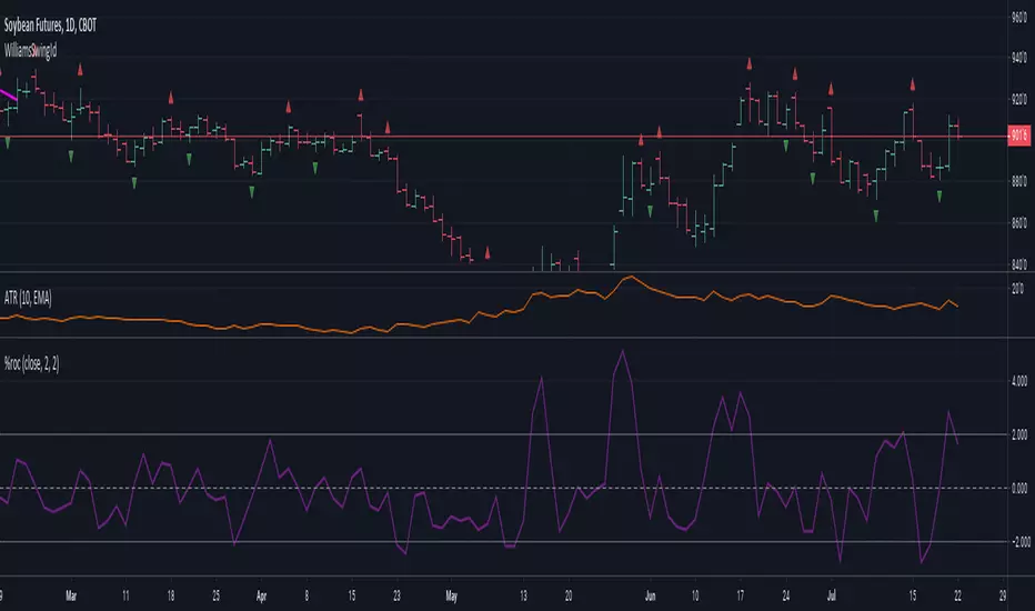
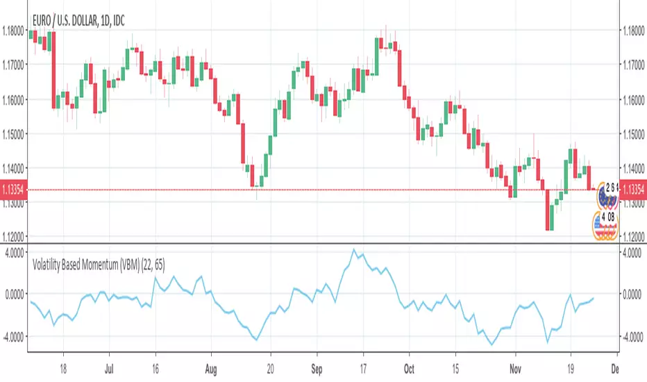
Volatility Based Momentum (VBM)The Volatility Based Momentum (VBM) indicator is a variation on the rate-of-change (ROC) indicator. Instead of expressing momentum in a percentage gain or loss, VBM normalizes momentum using the historical volatility of the underlying security.
The VBM indicator offers numerous benefits to traders who orient their trading around volatility. For these traders, VBM expresses momentum in a normalized, universally applicable ‘multiples of volatility’ (MoV) unit. Given the universal applicability of MoV, VBM is especially suited to traders whose trading incorporates numerous timeframes, different types of securities (e.g., stocks, Forex pairs), or the frequent comparison of momentum between multiple securities.
The calculation for a volatility based momentum (VBM) indicator is very similar to ROC, but divides by the security’s historical volatility instead. The average true range indicator (ATR) is used to compute historical volatility.
VBM(n,v) = (Close - Close n periods ago) / ATR(v periods)
For example, on a daily chart, VBM(22,65) calculates how many MoV price has increased or decreased over the last 22 trading days (approximately one calendar month). The second parameter is the number of periods to use with the ATR indicator to normalize the momentum in terms of volatility.
For more details, there is an article further describing VBM and its applicability versus ROC.
modificated rate of changeBased on ROC this indicator has been smoothed with filter and the zero line changed by a longer period of inverted ROC filtred as well . Buy/sell at the cross.
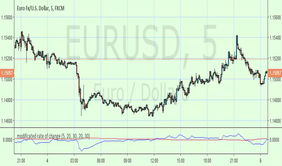
drnkk StrategyStrategy based upon combination with, ROC of Vortex, modified RSI, modified Price ROC,
Bu da mı gol değil?

Druckenmiller 2nd Order ROC [Acceleration]How to Read It (The User Guide)
This indicator doesn't just tell you if the price is going up or down; it tells you if the energy behind the move is growing or dying.
1. The Zero Line (The "Engine Check")
Think of the Zero Line as the difference between a car accelerating and coasting.
Crossing Above 0: The engine just kicked in. Buyers are stepping on the gas. Even if the candle is red, the internal momentum has turned bullish.
Action: Look for Longs.
Crossing Below 0: The engine is off. The car might still be rolling forward (price going up), but it's slowing down.
Action: Tighten Stops / Look for Shorts.
2. The Colors (The "Phase" Check)
🟢 Bright Green (Positive Acceleration):
Meaning: Price is moving up faster than before.
Action: Hold. This is the strongest part of the trend.
🟢 Faded Green (Positive Deceleration):
Meaning: Price is still moving up, but the "pop" is gone. It's struggling.
Action: Caution. Watch for a top.
🔴 Bright Red (Negative Acceleration):
Meaning: Panic. Price is crashing faster every candle.
Action: Hold Short / Stay Out.
🔴 Faded Red (Negative Deceleration):
Meaning: The selling is drying up. The crash is slowing down.
Action: Watch for a Bounce.
3. The "Druckenmiller Divergence" (The Money Shot)
This is the setup Stan Druckenmiller looks for—when the indicator disagrees with the price.
Bullish Reversal: Price makes a Lower Low (looks bad), BUT the Indicator makes a Higher Low (less red).
Translation: Sellers are exhausted. A rip your face off rally is imminent.
Bearish Reversal: Price makes a Higher High (looks good), BUT the Indicator makes a Lower High (less green).
Translation: Buyers are exhausted. The trend is hollow and about to collapse.
Pro Tip: Use this on Weekly or Monthly charts to find major market turns, just like Druckenmiller does. On 5-minute charts, it will be noisy.
