Trading Weekends Is a Dead-Man ZoneWeekend trading in crypto looks active on the surface, but the structure underneath is fragile. Liquidity thins, participation drops, and price becomes easier to move with relatively small orders. What appears to be opportunity is often noise amplified by absence of depth. This is why weekends quietly drain accounts rather than build them.
Institutional participation is minimal during weekends.
Many large players reduce exposure or remain inactive, which removes the stabilizing force that normally absorbs volatility and validates structure. Without that participation, levels lose reliability. Breakouts occur without follow-through. Reversals happen without warning. The market is not directional; it is reactive.
Spreads widen and order books thin. This increases slippage and distorts risk. Stops that would survive during active sessions are easily tagged. Entries that look precise on the chart fill poorly in reality. Execution quality degrades, even if the setup appears valid in hindsight.
Another issue is narrative vacuum. During the week, price responds to macro flows, funding dynamics, and session-based participation. On weekends, these drivers are largely absent. Price often rotates aimlessly or runs obvious liquidity pools without establishing commitment. Traders mistake movement for intent and become the liquidity that others exit against.
Psychology also shifts. Weekends invite boredom trading.
Without a structured routine, traders lower standards, widen assumptions, and take setups they would normally ignore. Losses feel smaller individually, but they accumulate through frequency and poor sequencing.
There are exceptions. High-impact events or structural carryover from a strong weekly close can create opportunity. These situations are rare and require reduced size and stricter confirmation. For most traders, restraint is the edge.
The market will still be there on Monday with clearer structure, deeper liquidity, and better execution conditions. Survival in trading is not about participation at all times. It is about choosing when conditions justify risk. Weekends rarely do.
Fundamental Analysis

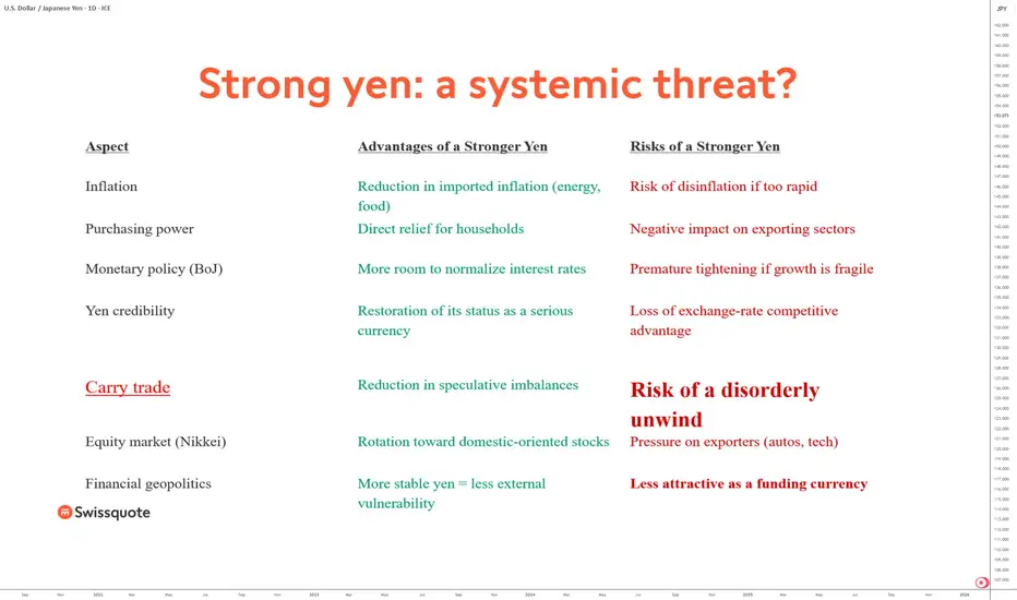
Yen rebound (JPY): a systemic threat?The Japanese yen is close to its lowest level in 40 years and has been the weakest currency in the FX market for several years. However, since the end of January 2026, it has shown a bullish impulse that could mark the beginning of a longer-term upward phase. Could such a regime shift in the yen’s trend represent a threat to Japan, the foreign exchange market, and global finance in general?
First, it is important to keep in mind that the recent rebound in the yen (JPY)—that is, the decline in USD/JPY since last Friday—does not yet change the yen’s underlying trend. The yen remains in a broader downtrend. However, if this underlying trend were to reverse from bearish to a new long-term bullish trend, then significant risks for global finance could indeed emerge. These risks are not driven by the yen rebounding per se, but rather by the speed and momentum of any potential appreciation of the Japanese currency.
The main systemic risk would stem from the unwinding of yen carry trade positions that are still outstanding. At the same time, it should not be overlooked that a yen rebound can also have positive effects, particularly for the Japanese economy, which is seeking to combat inflation.
Here is where the systemic risk to global finance could arise:
• If the yen rebounds too quickly (speed is the key factor), there could be a full unwinding of the approximately USD 200 billion in remaining yen carry trade positions, potentially triggering a global market sell-off
• If the yen rebounds sharply while Japanese interest rates continue to rise, a major source of global funding would disappear
• If the yen rebounds too strongly and too quickly, Japanese institutional investors may
repatriate capital invested abroad into domestic assets, triggering selling pressure on global equity markets
• From a technical perspective, USD/JPY must not fall below the 140 JPY support level
These risks must nevertheless be nuanced and placed within a broader macroeconomic context. A persistently weak yen has certainly supported the competitiveness of Japanese exports and boosted the profits of large listed companies, but it has also imported significant inflation, particularly in energy and food. In this context, a controlled rebound in the yen could instead be viewed as a factor of macroeconomic stabilization for Japan.
A stronger yen would help reduce imported inflation, improve the purchasing power of Japanese households, and restore some credibility to the Bank of Japan’s (BoJ) monetary policy, which has long been perceived as ultra-accommodative and isolated compared with other major central banks. It would also give the BoJ greater room to gradually normalize its interest rate policy without triggering an inflationary shock.
In summary, a yen rebound is not, in itself, a systemic threat. It only becomes potentially dangerous if it is too rapid, too violent, and leads to a sudden end of the yen carry trade. Under a central scenario of gradual normalization, a stronger yen could instead help reduce some of the imbalances accumulated over recent years, both in Japan and globally.
DISCLAIMER:
This content is intended for individuals who are familiar with financial markets and instruments and is for information purposes only. The presented idea (including market commentary, market data and observations) is not a work product of any research department of Swissquote or its affiliates. This material is intended to highlight market action and does not constitute investment, legal or tax advice. If you are a retail investor or lack experience in trading complex financial products, it is advisable to seek professional advice from licensed advisor before making any financial decisions.
This content is not intended to manipulate the market or encourage any specific financial behavior.
Swissquote makes no representation or warranty as to the quality, completeness, accuracy, comprehensiveness or non-infringement of such content. The views expressed are those of the consultant and are provided for educational purposes only. Any information provided relating to a product or market should not be construed as recommending an investment strategy or transaction. Past performance is not a guarantee of future results.
Swissquote and its employees and representatives shall in no event be held liable for any damages or losses arising directly or indirectly from decisions made on the basis of this content.
The use of any third-party brands or trademarks is for information only and does not imply endorsement by Swissquote, or that the trademark owner has authorised Swissquote to promote its products or services.
Swissquote is the marketing brand for the activities of Swissquote Bank Ltd (Switzerland) regulated by FINMA, Swissquote Capital Markets Limited regulated by CySEC (Cyprus), Swissquote Bank Europe SA (Luxembourg) regulated by the CSSF, Swissquote Ltd (UK) regulated by the FCA, Swissquote Financial Services (Malta) Ltd regulated by the Malta Financial Services Authority, Swissquote MEA Ltd. (UAE) regulated by the Dubai Financial Services Authority, Swissquote Pte Ltd (Singapore) regulated by the Monetary Authority of Singapore, Swissquote Asia Limited (Hong Kong) licensed by the Hong Kong Securities and Futures Commission (SFC) and Swissquote South Africa (Pty) Ltd supervised by the FSCA.
Products and services of Swissquote are only intended for those permitted to receive them under local law.
All investments carry a degree of risk. The risk of loss in trading or holding financial instruments can be substantial. The value of financial instruments, including but not limited to stocks, bonds, cryptocurrencies, and other assets, can fluctuate both upwards and downwards. There is a significant risk of financial loss when buying, selling, holding, staking, or investing in these instruments. SQBE makes no recommendations regarding any specific investment, transaction, or the use of any particular investment strategy.
CFDs are complex instruments and come with a high risk of losing money rapidly due to leverage. The vast majority of retail client accounts suffer capital losses when trading in CFDs. You should consider whether you understand how CFDs work and whether you can afford to take the high risk of losing your money.
Digital Assets are unregulated in most countries and consumer protection rules may not apply. As highly volatile speculative investments, Digital Assets are not suitable for investors without a high-risk tolerance. Make sure you understand each Digital Asset before you trade.
Cryptocurrencies are not considered legal tender in some jurisdictions and are subject to regulatory uncertainties.
The use of Internet-based systems can involve high risks, including, but not limited to, fraud, cyber-attacks, network and communication failures, as well as identity theft and phishing attacks related to crypto-assets.
Gold Is Not Crashing — Traders Are Being Forced OutWhat we are seeing in Gold right now is NOT normal volatility.
In my entire trading career, I have rarely seen:
• 400–500 pips moves on every 5-minute candle
• 4000+ pips drop in under 30 minutes
• Zero respect for structure, zones, or indicators
This is not technical selling.
This is forced liquidation.
Here’s what’s really happening:
• Over-leveraged traders getting margin called
• Brokers force-closing positions
• Algorithms accelerating panic
• Liquidity disappearing between candles
That’s why: ❌ No pullbacks
❌ No structure respect
❌ No “entry confirmation” works
If you are trading this like a normal market, you are already late.
🔑 Reality check:
When volatility explodes, survival matters more than accuracy.
This is not the time to: • Chase trades
• Predict bottoms
• Prove you’re right
This is the time to: • Reduce risk
• Reduce size
• Or stay out completely
💬 Serious question:
Are you trading this market —
or is this market trading you?

JINDAL STEEL looks potential upside 25-30%JINDAL STEEL having good numbers of results this quarter. also technically breaks rounding bottom formation on daily basis, also weekly if close above 1095.
As per this set up this can move towards 1400-1420 in next 6-8 month.
I am Not a SEBI Registered Research Analyst. Views shared are for educational purposes only. Please consult your financial advisor before investing.

FinEco For Dummies | The Economic Eco-System Simplified🟢 Intro For Financial Economics & The Financial Eco-Sytem For Dummies
This little book is not about predictions or strategies.
It’s about understanding how financial markets connect, interact, and move together.
If you can read capital flows, risk appetite, and macro relationships,
markets stop feeling random and start making sense.
Financial markets are a system.
Money flows between assets based on risk, growth, inflation, and policy.
This book explains those relationships in simple terms,
so you can understand the environment before making decisions.
Most traders focus on charts.
Few understand the environment those charts live in.
This little book lays out a simple framework for reading market conditions,
capital rotation, and risk behavior, without strategies or hype.
This is a foundation, not a strategy.
A simple guide to how stocks, bonds, currencies, commodities, and crypto
fit together inside the global financial system.
Markets are not random.
They react to incentives, risk, and expectations.
This book helps you see those forces clearly.
🟢 1 - The Big Picture: Markets as a Flow System
Before charts, indicators, or trades, financial markets should be understood as a system of flows, not isolated instruments. Every market, stocks, bonds, currencies, commodities, crypto, etc is simply capital moving between buckets. Nothing trades in a vacuum. When money flows into one place, it must flow out of another.
-
➡️ The Core Idea
Markets are a constant process of:
- Allocation
- Re-allocation
- Risk assessment
Investors are always asking, consciously or not:
“Where do I want my money to park right now?”
The answer changes with:
- Economic expectations
- Central bank policy
- Inflation / deflation fears
- Financial stability
- Geopolitical stress
- Liquidity conditions
Price is just the result of those decisions.
Risk Is the Organizing Principle
At the highest level, all markets organize around risk.
Capital rotates between:
- Risk-on assets → growth, leverage, expansion
- Risk-off assets → safety, preservation, defense
This is not emotional.
It is structural.
Institutions manage:
- Mandates
- Drawdowns
- Volatility targets
- Capital requirements
They must rotate.
-
➡️ The Two Master Regimes
Most market behavior can be simplified into two regimes:
➡️ 1. Risk-On Environment
Characteristics:
- Optimism about growth
- Liquidity is abundant
- Credit flows easily
- Volatility is tolerated
Money prefers:
- Equities (especially growth)
- High beta sectors
- Small & mid caps
- Emerging markets
- Cyclical commodities
➡️ 2. Risk-Off Environment
Characteristics:
- Uncertainty or stress
- Liquidity tightens
- Credit risk rises
- Volatility is avoided
Money prefers:
- Government bonds
- Strong reserve currencies
- Defensive equities
- Gold
- Cash equivalents
Most of the time, markets live between these two, rotating, not flipping instantly.
➡️ Why This Matters for Trading
If you don’t know which regime you’re in, technical setups lose meaning.
A perfect long breakout:
- Works beautifully in risk-on
- Fails constantly in risk-off
A short breakdown:
- Accelerates in risk-off
- Gets absorbed in risk-on
Your job is not to predict the future.
Your job is to identify the current state.
-
🟢 2 - Capital Rotation: How Money Actually Moves
Markets do not rise or fall as one unified object.
They rotate.
Capital is constantly shifting between:
- Sectors
- Asset classes
- Regions
- Risk profiles
This rotation is not random. It follows incentives.
-
➡️ Rotation vs Direction
A common beginner mistake is thinking:
“The market is bullish or bearish.”
In reality, markets are often:
- Bullish somewhere
- Bearish somewhere else
While headlines say “stocks are flat,” money may be:
- Leaving defensives
- Entering growth
- Rotating from large caps into small caps
- Moving from bonds into equities
- Or the opposite
Understanding where money is going matters more than knowing the index direction.
-
➡️ Why Rotation Exists
Large institutions:
- Cannot move all at once
- Cannot hold everything
- Must rebalance constantly
They rotate because of:
- Changing growth expectations
- Interest rate shifts
- Inflation outlook
- Volatility targets
- Risk management rules
This creates waves, not straight lines.
-
➡️ The Economic Cycle (Simplified)
While real life is messy, capital often behaves as if it follows a loose cycle:
Early Expansion
- Rates low or falling
- Liquidity improving
- Confidence returning
Capital prefers:
- Small caps
- Cyclicals
- Growth sectors
- High beta assets
Mid-Cycle
- Growth strong
- Earnings expanding
- Rates stable or slowly rising
Capital prefers:
- Large caps
- Technology
- Industrials
- Consumer discretionary
Late Cycle
- Inflation concerns
- Rates restrictive
- Margins pressured
Capital rotates into:
- Energy
- Materials
- Value
- Financials (if yield curve allows)
Stress / Contraction
- Growth uncertainty
- Credit risk rising
- Liquidity tightening
Capital hides in:
- Defensives
- Bonds
- Gold
- Cash (Liquidity tightening)
This is not a checklist, it’s a lens.
-
➡️ Why Broad Sector ETFs Matter
Broad ETFs allow you to:
- Observe rotation in real time
- See what is being rewarded
- Identify what is being abandoned
They act as market thermometers.
A single stock can lie.
A sector rarely does.
-
➡️ Relative Strength Is the Tell
The most important question is not:
“Is this going up?”
But:
“Is this outperforming other places capital could go?”
Outperformance = demand
Underperformance = avoidance
This relative behavior often appears before major market pivots.
-
➡️ Setting the Stage
From here, we’ll start breaking the market into functional blocks:
- Broad indices
- Sector ETFs
- Bonds
- Currencies
- Hard assets
- Others
Each block tells a different part of the story.
-
🟢 3 - Broad Market Structure: Who Leads, Who Follows
Before zooming into sectors, it’s critical to understand the hierarchy of the equity market itself.
Not all stocks matter equally.
Not all indices send the same signal.
Markets have leaders and followers.
-
➡️ The US Equity Market as a Pyramid
At the top of the pyramid sit the largest, most liquid companies.
At the bottom sit smaller, more fragile, higher-risk firms.
Large Caps
- Highly liquid
- Globally owned
- Institutional core holdings
They represent:
- Stability
- Capital preservation with growth
- Confidence in the system
Mid Caps
- More domestic exposure
- More growth-sensitive
- Less balance-sheet protection
They represent:
- Expansion
- Risk tolerance
- Economic optimism
Small Caps
- Least liquid
- Most rate-sensitive
- Highly dependent on credit conditions
They represent:
- Risk appetite
- Liquidity abundance
- Speculation tolerance
-
➡️ Why Size Matters
When confidence rises:
- Capital flows down the pyramid
- Large → Mid → Small
When stress appears:
- Capital flows up the pyramid
- Small → Mid → Large → Cash
This movement often happens before headlines change.
➡️ Reading the Market Through Indices
Broad indices act as regime filters:
SPY (S&P 500)
Represents large-cap US equity exposure
- Dominated by mega-cap tech and financials
Strength here means:
- Core capital is comfortable staying invested
- The system is stable enough to hold risk
RSP (Equal-Weight S&P 500)
Removes mega-cap dominance
- Shows participation breadth
If SPY rises but RSP lags:
- Leadership is narrow
- Risk is concentrated
- The rally is fragile
If RSP leads:
- Participation is broad
- Confidence is healthy
- Moves are more sustainable
-
➡️ Breadth Is Not a Detail - It’s a Warning System
Strong markets:
- Many stocks participating
- Many sectors contributing
- Leadership rotates smoothly
Weak markets:
- Few leaders
- Defensive hiding
- Sudden rotation spikes
Breadth deterioration often appears long before price collapses.
-
➡️ Why This Matters for Everything Else
Equity leadership sets the tone for:
- Sector performance
- Currency flows
- Bond behavior
- Commodity demand
If equities are unhealthy internally, risk assets elsewhere struggle to hold gains.
-
➡️ Key Takeaway
Markets don’t break all at once.
They weaken from the inside out.
If you learn to read:
- Size
- Breadth
- Leadership
You stop reacting and start anticipating.
-
🟢 4 - Sector ETFs: Reading the Economy Through Capital
KRE — Regional Banks
US regional banks, credit-sensitive, domestic lending.
Best in: Early recovery, rate cuts, steepening yield curve.
Struggles in: Tight liquidity, stress, rising defaults.
ITB — Homebuilders
US residential construction and housing demand.
Best in: Falling rates, easing financial conditions.
Struggles in: Rising yields, affordability stress.
SMH — Semiconductors
Global chipmakers, cyclical growth, capex-driven.
Best in: Expansion, liquidity growth, tech-led cycles.
Struggles in: Hard slowdowns, demand shocks.
XME — Metals & Mining
Steel, miners, raw materials.
Best in: Reflation, infrastructure cycles, USD weakness.
Struggles in: Deflation, global slowdown.
XLRE — Real Estate
REITs, income and rate-sensitive assets.
Best in: Falling yields, stable growth.
Struggles in: Rising rates, credit stress.
XLY — Consumer Discretionary
Non-essential spending (retail, autos, leisure).
Best in: Strong consumer, expansion phases.
Struggles in: Recessions, confidence drops.
EBIZ — E-Commerce / Digital Consumption
Online retail and digital consumer platforms.
Best in: Growth + digital shift, USD weakness.
Struggles in: Consumer pullbacks, tightening liquidity.
XLK — Technology
Large-cap US tech, growth and duration exposure.
Best in: Liquidity expansion, falling rates.
Struggles in: Tight policy, rising real yields.
XLE — Energy
Oil & gas producers and services.
Best in: Reflation, supply constraints, USD weakness.
Struggles in: Demand destruction, growth shocks.
XLB — Materials
Chemicals, construction materials, inputs.
Best in: Early-cycle recovery, reflation.
Struggles in: Late-cycle slowdowns.
RSP — Equal-Weight S&P 500
Broad market without mega-cap dominance.
Best in: Healthy, broad-based expansions.
Struggles in: Narrow leadership, defensive markets.
SPY — S&P 500
US large-cap benchmark.
Best in: Most regimes, reflects overall risk appetite.
Struggles in: Systemic shocks.
XLI — Industrials
Manufacturing, transport, capital goods.
Best in: Expansion, infrastructure, global growth.
Struggles in: Recessions, trade slowdowns.
XLF — Financials
Banks, insurers, financial services.
Best in: Steep yield curve, economic growth.
Struggles in: Credit stress, inverted curves.
XLC — Communication Services
Media, telecom, platforms.
Best in: Growth environments, ad spending cycles.
Struggles in: Economic slowdowns.
IGV — Software
Enterprise software and digital services.
Best in: Liquidity expansion, productivity cycles.
Struggles in: Rate shocks, valuation compression.
XLV — Healthcare
Pharma, biotech, medical services.
Best in: Defensive regimes, late cycle.
Struggles in: High-risk-on rotations.
XLU — Utilities
Regulated utilities, income-focused.
Best in: Risk-off, falling yields.
Struggles in: Rising rates, strong growth cycles.
XLP — Consumer Staples
Essentials (food, household goods).
Best in: Defensive, late-cycle, risk-off.
Struggles in: Strong risk-on rotations.
Once you understand broad market structure, the next layer is sectors.
Sector ETFs are not just industries.
They are expressions of economic belief.
Each sector answers a different question:
- Growth or safety?
- Inflation or deflation?
- Rates up or rates down?
- Confidence or caution?
By watching sector behavior, you can see what investors are preparing for, not what they are reacting to.
-
➡️ Sectors as Economic Sensors
Sectors move differently because:
- They respond differently to rates
- They depend differently on credit
- They react differently to inflation and demand
This makes them ideal tools for:
- Identifying rotation
- Confirming or rejecting index moves
- Spotting regime changes early
➡️ 1. Risk-Oriented Sectors (Risk-On)
These sectors perform best when:
- Liquidity is abundant
- Growth expectations are rising
- Investors are willing to take risk
Technology - XLK / IGV / EBIZ
- Growth-driven
- Highly rate-sensitive
- Dependent on future earnings
Strength implies:
- Falling or stable rates
- Confidence in innovation and growth
- Risk-on environment
Weakness implies:
- Rising real yields
- Liquidity stress
- De-risking behavior
Consumer Discretionary - XLY
- Depends on consumer confidence
- Sensitive to employment and credit
Strength implies:
- Healthy consumers
- Economic expansion
- Optimism about income growth
Weakness implies:
- Caution
- Demand slowdown
- Household stress
➡️ Cyclical / Expansion Sectors
These sectors benefit from economic activity itself.
Industrials - XLI
- Linked to manufacturing and infrastructure
- Sensitive to growth and capex cycles
Strength implies:
- Expansion
- Business investment
- Trade and logistics activity
Materials - XLB / Metals & Mining - XME
- Sensitive to inflation and construction
- Linked to global demand
Strength implies:
- Rising inflation expectations
- Commodity demand
- Late-cycle or reflation themes
Energy - XLE
- Tied to inflation and geopolitics
- Sensitive to supply constraints
Strength implies:
- Inflation pressure
- Tight energy markets
- Often late-cycle behavior
-
➡️ 2. Defensive Sectors (Risk-Off)
These sectors attract capital when:
- Growth is uncertain
- Volatility rises
- Preservation matters more than return
Healthcare - XLV
- Inelastic demand
- Stable cash flows
Strength implies:
- Defensive rotation
- Risk reduction
- Uncertainty ahead
Consumer Staples - XLP
- Everyday necessities
- Low growth but high stability
Strength implies:
- Capital hiding
- Caution
- Late-cycle or stress environment
Utilities - XLU
- Yield-oriented
- Rate-sensitive
Strength implies:
- Demand for safety and income
- Falling rates or risk-off mood
-
➡️ Interest-Rate Sensitive Sectors
Some sectors are less about growth and more about rates.
Real Estate - XLRE
- Highly sensitive to interest rates
- Dependent on financing costs
Strength implies:
- Falling or stabilizing rates
- Yield-seeking behavior
Weakness implies:
- Rising rates
- Credit stress
Financials - XLF / KRE
- Banks reflect system health
- Credit creation and yield curve dependent
Strength implies:
- Healthy lending environment
- Confidence in the financial system
Weakness implies:
- Credit stress
- Yield curve pressure
- Systemic caution
-
➡️ Breadth and Rotation Inside Sectors
A healthy market:
- Multiple sectors leading
- Smooth rotation
- No single sector carrying the index
An unhealthy market:
- Narrow leadership
- Defensive outperformance
- Violent sector rotations
-
➡️ Key Takeaway
Sectors tell you why the market is moving.
Index price tells you that it moved.
Sector behavior tells you what investors believe.
-
➡️ Market Regime Cheat-Sheet
How to Read Sector ETFs in Context
🟢 Risk-On / Expansion
Liquidity flowing, growth rewarded
SMH — Semiconductors (cyclical tech leadership)
XLK — Technology (liquidity + duration)
IGV — Software (productivity, growth)
XLY — Consumer Discretionary (strong consumer)
EBIZ — E-Commerce (digital spending)
XLC — Communication Services (ads, platforms)
Macro backdrop:
- Falling or stable rates
- Easy financial conditions
- Weak or stable USD
- Strong equity breadth
-
🟡 Reflation / Early Cycle
Growth + inflation expectations rising
XLE — Energy (oil, supply constraints)
XME — Metals & Mining (raw materials)
XLB — Materials (inputs, construction)
XLI — Industrials (capex, infrastructure)
ITB — Homebuilders (rate relief + demand)
Macro backdrop:
- Inflation stabilizing or rising
- USD weakness
- Yield curve steepening
- Commodity strength
-
🔵 Broad & Healthy Market
Participation matters more than leaders
RSP — Equal-Weight S&P 500
SPY — Market benchmark
Macro backdrop:
- Balanced growth
- No extreme policy pressure
- Internal market strength
- Rotation instead of liquidation
-
🟠 Financial Sensitivity
Rates, credit, curve shape matter
XLF — Financials (steep curve, growth)
KRE — Regional Banks (credit health)
XLRE — Real Estate (rate sensitivity)
Macro backdrop:
Rate cuts help
Credit stability required
Stress shows early here
-
🔴 Defensive / Risk-Off
Capital preservation, not growth
XLV — Healthcare
XLP — Consumer Staples
XLU — Utilities
Macro backdrop:
- Tight liquidity
- Economic uncertainty
- Rising volatility
- Capital rotates, doesn’t disappear
How to Use This Cheat-Sheet:
- Leadership = regime signal
- Rotation ≠ crash
- Defensives leading = caution
- Cyclicals + tech leading = expansion
- Banks & housing weaken first in stress
-
🟢 5 - Bonds and Central Banks: The Gravity of Markets
If equities are the expression of confidence,
bonds are the constraint.
No market ignores bonds for long.
Interest rates determine:
- The cost of money
- The price of leverage
- The value of future cash flows
- The tolerance for risk
This makes bonds the gravitational force of financial markets.
-
➡️ Why Bonds Matter More Than Headlines
Stocks can stay irrational for a while.
Bonds can not.
Bond markets are dominated by:
- Institutions
- Governments
- Pension funds
- Central banks
They reflect:
- Inflation expectations
- Growth expectations
- Trust in policymakers
When bonds move, everything else eventually follows.
-
➡️ US Treasuries - The Global Benchmark
US Treasuries are the foundation of:
- Global pricing
- Risk-free rates
- Collateral systems
Rising yields mean:
- Tighter financial conditions
- Higher discount rates
- Pressure on growth assets
Falling yields mean:
- Easier conditions
- Support for risk-taking
- Relief for leveraged assets
-
➡️ Short-Term vs Long-Term Yields
The shape of the yield curve matters.
Rising short-term yields:
- Reflect central bank tightening
- Increase funding stress
- Pressure equities and credit
Rising long-term yields:
- Reflect inflation or growth expectations
- Hurt duration-sensitive assets
- Strengthen the currency
Falling long-term yields:
- Signal slowing growth or stress
- Support defensives and gold
-
➡️ The Federal Reserve - Liquidity Manager
The Fed does not control markets directly.
It controls liquidity conditions.
Through:
- Policy rates
- Balance sheet operations
- Forward guidance
The Fed influences:
- Risk appetite
- Credit creation
- Volatility tolerance
Markets often move in anticipation of Fed actions, not after them.
-
➡️ Japan: The Silent Anchor (BoJ & JGBs)
Japan plays a unique role in global markets.
- Ultra-low rates
- Yield curve control history
- Massive domestic savings
Japanese bonds (JGBs) act as:
- A funding benchmark
- A pressure valve for global yields
When Japanese yields rise:
- Global yields tend to follow
- Yen strengthens
- Risk assets feel pressure
This is why Japan matters even if you don’t trade it directly.
-
➡️ Fed vs BoJ - A Critical Relationship
When:
- US rates rise
- Japanese rates stay suppressed
Capital flows:
- Into USD
- Out of JPY
- Into risk assets funded by cheap yen
When that gap narrows:
- Carry trades unwind
- Volatility increases
- Risk assets struggle
-
➡️ Key Takeaway
Bonds tell you:
- How tight or loose the system is
- Whether risk-taking is rewarded or punished
- When markets are approaching stress
Ignore bonds, and everything else becomes noise.
-
🟢 6 - Currencies and FX Indexes: The Language of Capital Flows
Currencies are often misunderstood as “forex trades.”
In reality, currencies are statements of preference.
They show:
- Where capital feels safest
- Where returns are most attractive
- Which economies are trusted
- Which risks are being avoided
Currencies don’t move because of opinions.
They move because of flows.
-
➡️ Why Currencies Matter Even If You Don’t Trade FX
Every asset is priced in a currency.
That means:
- Stocks
- Bonds
- Commodities
- Crypto (later)
Are all influenced by currency strength and weakness.
If you ignore currencies, you miss:
- Hidden tailwinds
- Silent headwinds
- False breakouts caused by FX pressure
-
➡️ The US Dollar (DXY) - Global Liquidity Thermometer
The US dollar is:
- The world’s reserve currency
- The primary funding currency
- The denominator for global trade
A rising USD usually means:
- Tighter global liquidity
- Pressure on risk assets
- Stress for emerging markets
- Headwinds for commodities
A falling USD usually means:
- Easier financial conditions
- Support for equities
- Tailwinds for commodities and risk assets
The dollar is not “bullish” or “bearish.”
It is restrictive or permissive.
-
➡️ Safe-Haven Currencies - JPY and CHF
Some currencies strengthen not because of growth, but because of fear.
Japanese Yen (JPY)
- Historically used for funding
- Ultra-low rate environment
JPY strength implies:
- Risk-off behavior
- Carry trade unwinds
- Stress in global markets
JPY weakness implies:
- Risk-on
- Leverage expansion
- Yield chasing
Swiss Franc (CHF)
- Capital preservation currency
- Financial system trust play
CHF strength implies:
- Capital hiding
- Defensive positioning
- Systemic caution
Risk-Sensitive Currencies
Other currencies strengthen when:
- Growth is strong
- Commodities are in demand
- Risk appetite is healthy
These act as confirmation tools, not drivers.
Weakness here alongside strong equities is often a warning sign.
-
➡️ Currency Indexes as Regime Filters
Watching individual FX pairs can be noisy.
Indexes simplify the message.
Currency indexes help you:
- Identify broad strength or weakness
- Avoid pair-specific distortions
- See regime shifts early
If:
- USD strengthens
- JPY strengthens
- CHF strengthens
That combination rarely supports sustained risk-on behavior.
➡️ Currencies and Equity Behavior
Healthy risk environments usually show:
- Weak or stable USD
- Weak JPY
- Broad equity participation
Stress environments often show:
- Strong USD
- Strong JPY or CHF
- Narrow or defensive equity leadership
Currencies often lead equities, not the other way around.
➡️ Key Takeaway
Currencies are the nervous system of global markets.
They transmit:
- Stress
- Confidence
- Liquidity shifts
If you listen to them, markets stop surprising you.
-
➡️ Currency Regime Cheat-Sheet
*How to Read XY Indices in a Macro Context
-
USDX / DXY — US Dollar Index
Global reserve, liquidity gauge
Strong DXY → global liquidity tightens
Weak DXY → risk assets breathe
Strength signals:
- Risk-off
- Higher real yields
- Global stress
Weakness signals:
- Risk-on
- Commodity support
- EM + crypto tailwind
-
JXY — Japanese Yen Index
Carry trade & volatility trigger
Weak JPY → leverage, risk-taking
Strong JPY → carry unwind, stress
Watch for:
- USDJPY turning points
- BoJ policy shifts
- Global volatility spikes
Yen strength often precedes:
- Equity pullbacks
- Tech weakness
- Crypto drawdowns
-
CXY — Canadian Dollar Index
Commodity & energy proxy
Tracks oil, metals, global growth
Pro-cyclical currency
Strength signals:
- Risk-on
- Commodity demand
- Inflation expectations
Weakness signals:
- Growth slowdown
- Commodity pressure
-
EXY — Euro Index
Growth vs stability balance
Sensitive to global trade
Often moves opposite DXY
Strength signals:
- Global growth optimism
- Risk-on rotation
Weakness signals:
Fragmentation risk
- Banking stress
- Energy shocks
-
BXY — British Pound Index
High beta developed-market currency
Volatile, sentiment-driven
Sensitive to rates & growth
Strength signals:
- Risk-on
- Hawkish BoE expectations
Weakness signals:
- Risk-off
- Political or fiscal stress
-
AXY — Australian Dollar Index
China & global growth barometer
Closely tied to commodities & China
One of the best early growth signals
Strength signals:
- Expansion
- Commodity demand
- Risk-on
Weakness signals:
- China slowdown
- Risk aversion
-
NXY — New Zealand Dollar Index
Pure risk appetite signal
Thin liquidity, high beta
Amplifies global sentiment
Strength signals:
- Risk-on extremes
- Yield-seeking behavior
Weakness signals:
- Flight to safety
- Liquidity stress
-
➡️ How to Read *XYs Together
DXY + JXY rising → risk-off, deleveraging
DXY down + CXY / AXY up → reflation, commodities
JPY leading strength → early warning
AUD / CAD leading → growth confidence
Currencies move first.
Assets react later.
-
➡️ Key Takeaway
XY indices are not trades.
They are context engines.
If you know which currencies are gaining strength,
you know where capital is moving — and why.
Context first.
Positioning second.
-
🟢 7 - Gold and Hard Assets: Trust, Fear, and Real Value
Gold is not a growth asset.
It is not a risk asset.
It is not a productive asset.
Gold is a belief asset.
It reflects:
- Trust in money
- Confidence in institutions
- Fear of debasement
- Desire for permanence
➡️ Why Gold Exists in Modern Markets
Gold does not compete with stocks.
It competes with currencies and bonds.
Gold becomes attractive when:
- Real yields fall
- Currency purchasing power is questioned
- Financial stability is doubted
It is an alternative to:
- Paper promises
- Credit systems
- Central bank credibility
-
➡️ Gold vs Nominal Yields (Coupon rate on a bond)
A common mistake is watching gold against nominal rates.
Gold responds primarily to:
- Real yields (rates minus inflation)
- Currency strength, especially USD
Rising real yields:
- Pressure gold
- Favor cash and bonds
Falling real yields:
- Support gold
- Signal hidden stress or easing
Gold often rises before inflation becomes obvious.
- Gold and the US Dollar
- Gold and USD often move inversely.
Strong USD:
- Makes gold expensive globally
- Reduces gold demand
Weak USD:
- Supports gold
- Signals easier financial conditions
When gold rises despite a strong USD:
- That is a warning signal
- Stress or distrust is increasing
-
➡️ Gold as a Stress Barometer
Gold strength often appears when:
- Financials weaken
- Credit risk rises
- Volatility increases
- Central banks lose control narratives
Gold does not panic.
It prepares.
-
➡️ Hard Assets Beyond Gold
Other hard assets (commodities, metals) behave differently:
- They depend on demand
- They are growth-sensitive
- They can fall in deflationary stress
Gold is unique because:
- It does not depend on growth
- It does not default
- It does not dilute
-
➡️ Gold in a Healthy Market
In strong risk-on environments:
- Gold often lags
- Capital prefers productive assets
In unstable or late-cycle environments:
- Gold begins to lead
- Quietly at first
Gold strength during equity rallies is often a yellow flag.
-
➡️ Key Takeaway
Gold measures confidence in the system itself.
It does not chase returns.
It waits for doubt.
If gold starts outperforming while risk assets struggle, the market is telling you something important.
-
🟢 8 - Silver, Copper, and Oil: The Economy’s Lie Detectors
If gold measures trust,
Industrial commodities measure reality.
Silver, copper, and oil don’t care about narratives.
They respond to:
- Demand
- Production
- Energy use
- Industrial activity
They tell you whether the economy is actually functioning, not whether markets hope it is.
-
➡️ Silver - The Hybrid Asset
Silver sits between two worlds:
- Monetary metal
- Industrial commodity
Because of this, silver often behaves as:
- A leveraged version of gold when confidence is high
- An industrial proxy when growth is strong
Silver strength implies:
- Inflation expectations
- Manufacturing demand
- Liquidity abundance
Silver weakness implies:
- Industrial slowdown
- Deflationary pressure
- Liquidity stress
Silver usually:
- Lags gold in early stress
- Leads gold in reflation
Gold moves on fear.
Silver moves when fear meets demand.
-
➡️ Dr. Copper - The Doctor of the Economy
Copper is often called:
“The metal with a PhD in economics”
That’s because copper demand is tied directly to:
- Construction
- Infrastructure
- Manufacturing
- Electrification
Copper strength implies:
- Real economic activity
- Capital investment
- Expansionary conditions
Copper weakness implies:
- Demand destruction
- Growth slowdown
- Recession risk
Copper rarely lies.
If equities rally while copper falls, something is off.
-
➡️ Copper vs Equities
Healthy expansions usually show:
- Rising equities
- Rising copper
- Rising industrial demand
Danger zones appear when:
- Equities rise
- Copper falls
- Liquidity-driven rallies dominate
That divergence often precedes:
- Growth disappointments
- Equity corrections
- Risk repricing
-
➡️ Oil - The Lifeblood of the System
Oil is not just a commodity.
It is energy, and energy underpins everything.
Oil prices reflect:
- Global demand
- Transportation activity
- Industrial throughput
- Geopolitical stress
Rising oil can mean:
- Strong demand
- Inflation pressure
- Supply constraints
Falling oil can mean:
- Demand destruction
- Economic slowdown
- Deflationary forces
Context matters more than direction.
-
➡️ Oil and Inflation
Oil spikes often:
- Pressure consumers
- Hurt margins
- Force central bank responses
Sustained high oil prices:
- Act like a tax on growth
- Accelerate late-cycle dynamics
Oil collapses often:
- Signal recession
- Precede central bank easing
Putting Them Together
- Gold asks: Do you trust the system?
- Silver asks: Is inflation and demand building?
- Copper asks: Is the economy actually growing?
- Oil asks: Can the system afford this energy cost?
When all agree, markets trend smoothly.
When they diverge, volatility follows.
-
➡️ Key Takeaway
Commodities expose the difference between financial optimism and economic reality.
Equities can float on liquidity.
Commodities need demand.
If hard assets stop confirming financial markets, risk is being mispriced.
-
🟢 9 - Volatility and Options: Stress Beneath the Surface
Price tells you where markets go.
Volatility tells you how they feel about it.
The VIX and the options market are not predictors.
They are emotion and insurance markets.
They show:
- Fear
- Complacency
- Protection demand
- Risk tolerance
-
➡️ What the VIX Actually Is
The VIX measures:
- Expected volatility in the S&P 500
- Derived from option prices
- Forward-looking, not historical
Think of the VIX as:
- The price of fear
- The cost of insurance
High fear = expensive protection
Low fear = cheap protection
-
➡️ What High and Low VIX Mean
Low VIX
- Complacency
- Confidence
- Cheap leverage
- Risk-taking encouraged
This usually aligns with:
- Risk-on environments
- Strong equity trends
- Narrow pullbacks
But extremely low VIX can mean:
- Fragility
- Overconfidence
- Vulnerability to shocks
High VIX
- Fear
- Demand for protection
- Forced hedging
This usually aligns with:
- Risk-off environments
- Equity stress
- Violent price moves
But high VIX can also mean:
- Capitulation
- Opportunity
- Panic already priced in
-
➡️ Context matters.
Why VIX Is a Confirmation Tool, Not a Signal
The VIX should not be traded as a direction indicator.
Instead, it helps answer questions like:
- Is fear rising or falling?
- Is this move relaxed or stressed?
- Are investors hedging or chasing?
Examples:
- Rising equities + rising VIX = unhealthy
- Falling equities + falling VIX = complacent risk
- Falling equities + spiking VIX = stress or panic
-
➡️ Broad Options Market: Insurance Demand
Options markets reflect:
- Where traders fear losses
- Where institutions hedge exposure
- Where risk is concentrated
Heavy put demand implies:
- Protection seeking
- Defensive positioning
Heavy call demand implies:
- Speculation
- Momentum chasing
You don’t need details.
You just need to know which side is desperate.
-
➡️ Volatility and Market Regimes
Healthy markets usually show:
- Moderate or declining volatility
- Predictable rotations
- Orderly pullbacks
Unhealthy markets show:
- Volatility spikes
- Sudden regime shifts
- Failed breakouts
Volatility often changes first, price follows later.
-
➡️ Why This Belongs in the Foundation
VIX and options help you:
- Avoid false confidence
- Recognize fragile rallies
- Respect stressed markets
- Adjust expectations
They don’t tell you what to trade.
They tell you how careful to be.
-
➡️ Key Takeaway
Volatility measures psychology under pressure.
When price and volatility agree, trends persist.
When they diverge, caution is warranted.
Used simply, volatility adds clarity, not noise.
-
🟢 10 - Crypto: Liquidity, Speculation, and Confidence
Crypto is not a replacement for money.
It is not a hedge like gold.
It is not a stock.
Crypto is a reflection of liquidity, trust, and speculative appetite.
To understand crypto, you must stop asking:
“Is it valuable?”
And start asking:
“Why does capital flow here now?”
-
➡️ What Crypto Represents in the Financial Ecosystem
Crypto sits at the edge of the system.
It attracts capital when:
- Liquidity is abundant
- Trust in traditional systems weakens
- Speculation is rewarded
- Regulation feels distant
It loses capital when:
- Liquidity tightens
- Risk appetite falls
- Funding costs rise
- Fear replaces optimism
Crypto does not create liquidity.
It absorbs excess liquidity.
-
➡️ Crypto Is a Risk-On Asset
Despite its narratives, crypto behaves mostly as:
- High beta (volatile)
- Leverage-sensitive
- Confidence-dependent
Strong crypto markets usually align with:
- Weak or falling USD
- Easy financial conditions
- Tech leadership
- High risk tolerance
Weak crypto markets usually align with:
- Strong USD
- Rising yields
- Liquidity stress
- Risk aversion
Crypto exaggerates what markets already feel.
-
➡️ Bitcoin vs the Rest
Bitcoin often behaves differently from smaller crypto assets.
Bitcoin represents:
- The most liquid crypto asset
- A proxy for crypto confidence
- A store of belief, not value
Smaller crypto assets represent:
- Speculation
- Excess risk appetite
- Leverage
In stress:
- Bitcoin holds better
- Smaller assets collapse
This mirrors:
- Large caps vs small caps in equities
-
➡️ Crypto and Trust
Crypto rallies often coincide with:
- Distrust in institutions
- Banking stress
- Monetary uncertainty
- Policy confusion
But unlike gold:
- Crypto requires liquidity
- Crypto requires participation
- Crypto collapses without buyers
Gold survives fear.
Crypto needs belief and liquidity.
-
➡️ Crypto as a Timing Tool
Crypto often:
- Moves early in risk-on phases
- Peaks before broader markets
- Collapses faster in risk-off events
This makes crypto useful as:
- A sentiment amplifier
- A liquidity stress detector
Crypto rarely causes market turns.
It reveals them.
-
➡️ Why Crypto Should Be Side-eyed as Traditional Investor
Crypto helps answer:
- Are people willing to speculate?
- Is liquidity leaking out of the system?
- Is confidence rising or cracking?
Crypto is not the center of the system.
It is the canary at the edge.
-
➡️ Key Takeaway
Crypto measures belief under abundance.
When money is cheap and confidence is high, crypto thrives.
When money tightens or fear rises, crypto breaks first.
It is not a leader.
It is a mirror.
-
🟢 11 - High Impact News & The Weekly Economic Calendar
Financial markets don’t move randomly.
They move around expectations and those expectations are challenged by scheduled news.
High impact news is not about surprise headlines.
It’s about known events that can change how markets price the future.
-
➡️ What Is “High Impact” News?
High impact news is data or events that can:
- Shift central bank policy expectations
- Reprice interest rates
- Change currency flows
- Alter risk-on / risk-off behavior
Traders don’t trade the number itself.
They trade the difference between expectations and reality.
-
➡️ Why the Weekly Calendar Matters
The economic calendar tells you:
- When volatility risk is highest
- When trends can accelerate or break
- When fakeouts are more likely
Markets are often quiet before big releases
and violent after them.
Knowing the calendar helps you:
- Avoid bad timing
- Size risk correctly
- Understand sudden moves
-
➡️ Tier 1 - The Market Movers
These events can move everything at once.
Central Bank Rate Decisions (Fed, ECB, BoJ, etc.)
What they control:
- Interest rates
- Liquidity conditions
- Financial stability
Why they matter:
- Rates affect currencies
- Rates affect bonds
- Rates affect equity valuations
Markets react more to:
- Forward guidance
- Tone of communication
- Changes in wording
Rates don’t need to change for markets to move.
-
➡️ Non-Farm Payrolls (NFP)
What it measures:
- US job creation
- Labor market strength
Why it matters:
- Direct input for Fed policy
- Strong labor supports higher rates
Key components:
- Wage growth
- Participation rate
- Unemployment rate
Typical reactions:
- Strong NFP → USD up, yields up
- Weak NFP → USD down, yields down
Equities react based on what it means for rates, not jobs.
-
➡️ CPI / Inflation Data
What it measures:
- Price pressure in the economy
Why it matters:
- Determines rate direction
- Affects real yields
- Impacts purchasing power
Typical reactions:
- Hot CPI → bonds down, USD up, equities pressured
- Cool CPI → bonds up, USD down, equities supported
Inflation surprises ripple across all markets.
-
➡️ Tier 2 - Growth & Activity Signals
These shape the broader macro narrative.
➡️ PMI / ISM Data
What it measures:
- Business activity
- Economic momentum
Key level:
- Above 50 = expansion
- Below 50 = contraction
Implications:
- Strong PMI → cyclicals, commodities, equities benefit
- Weak PMI → defensives, bonds, safe havens benefit
-
➡️ Retail Sales
What it measures:
- Consumer demand
Why it matters:
- Consumption drives growth
- Confirms economic strength or slowdown
Strong sales support growth narratives
Weak sales raise recession risk.
-
➡️ GDP
What it measures:
- Overall economic output
Why it matters:
- Confirms trends already in motion
GDP rarely shocks markets.
Markets usually price it before it’s released.
➡️ Tier 3 - Context & Confirmation
These rarely move markets alone but add depth.
Includes:
- Housing data
- Consumer sentiment
- Trade balance
- Regional surveys
Useful for:
- Macro confirmation
- Long-term assessment
- Narrative validation
-
➡️ How Traders Actually Use High Impact News
Professionals focus on:
- Expectations vs outcomes
- Market reaction, not logic
- Yield and currency response first
They often:
- Reduce risk before events
- Wait for post-news structure
- Trade continuation, not the spike
-
➡️ Key Takeaways
High impact news:
- Sets volatility windows
- Tests market narratives
- Exposes weak positioning
The calendar doesn’t tell you what to trade.
It tells you when risk is highest.
If you know:
- What’s coming
- Why it matters
- Who it affects
You’re already ahead of most participants.
-
🟢 12 - Politics & Policy (For Dummies)
Politics matters to markets only when it affects:
- Growth
- Inflation
- Liquidity
- Confidence
Markets do not care about ideology.
They care about impact.
-
➡️ The Three Policy Buckets That Move Markets
1. Monetary Policy (Central Banks)
Handled by:
- Federal Reserve (US)
- ECB (Europe)
- BOJ (Japan)
- Others
Main tools:
- Interest rates
- Balance sheet size (QE / QT)
- Forward guidance
Typical market reactions:
- Rate cuts → risk-on, weaker currency, bonds up
- Rate hikes → risk-off, stronger currency, bonds down
- Dovish tone → equities up
- Hawkish tone → equities down
-
➡️ This is the most powerful policy lever.
2. Fiscal Policy (Governments)
Handled by:
- Governments
- Parliaments
- Treasuries
Includes:
- Government spending
- Tax cuts or hikes
- Stimulus packages
- Infrastructure plans
- Defense budgets
Typical market reactions:
- Stimulus → growth assets up, inflation expectations up
- Austerity → growth slows, defensive assets favored
- Large deficits → bond supply pressure, currency sensitivity
Fiscal policy works slower than monetary policy but lasts longer.
-
➡️ 3. Regulatory & Geopolitical Policy
Includes:
- Trade policy
- Sanctions
- Industrial policy
- Energy policy
- Tech regulation
Typical reactions:
- Protectionism → inflation risk, supply chain stress
- Deregulation → sector-specific rallies
- Geopolitical tension → commodities, defense, USD strength
- Stability → risk assets favored
Markets price uncertainty, not morality.
-
➡️ Key Takeaway
Politics matters only through:
- Rates
- Spending
- Rules
- Stability
Ignore the noise.
Track the economic consequences.
-
🟢 13 - Transmission Channels (Final)
Now you understand the engine.
This section explains where the effects show up.
-
➡️ Housing Markets
Sensitive to:
- Interest rates
- Credit availability
- Employment
Why it matters:
- Major household asset
- Wealth effect on consumption
- Banking system exposure
Typical signals:
- Falling housing → economic slowdown
- Rising housing → consumer confidence
-
➡️ Pensions & Long-Term Capital
Sensitive to:
- Bond yields
- Equity performance
- Demographics
Why it matters:
- Forces long-term asset allocation
- Drives demand for bonds and equities
- Creates slow, structural flows
Pensions don’t trade headlines.
They rebalance trends.
-
➡️ Government Debt
Sensitive to:
- Rates
- Inflation
- Confidence in institutions
Why it matters:
- Competes with private capital
- Influences currency credibility
- Affects future policy flexibility
Debt becomes a problem when:
- Growth < interest costs
- Confidence weakens
-
➡️ Trade & Global Capital Flows
Sensitive to:
- Currency strength
- Relative growth
- Yield differentials
Why it matters:
- Explains currency trends
- Explains sector winners
- Explains regional outperformance
Money flows where:
- Returns are higher
- Risk is perceived lower
-
➡️ Putting It All Together
Markets are not random.
They are a feedback system between:
- Policy
- Growth
- Inflation
- Risk appetite
- Capital flows
If you understand:
- Who controls liquidity
- Where growth is accelerating
- Which assets signal stress
You don’t need predictions.
You read the system!
The end.

How to Trade FOMC Days – Smart Money FrameworkFOMC days consistently produce some of the most volatile price movements in the market. The key is not predicting the news, but understanding how liquidity behaves around it. Below is a structured approach based on Smart Money Concepts.
1. Before the Release
Price typically consolidates and builds liquidity on both sides of the range.
Key steps:
Mark previous day’s high/low
Identify Asia range liquidity
Note premium/discount zones
Avoid early trades — the market often engineers traps before the announcement
2. During the Release (14:00–14:30 ET)
This is the most dangerous window.
Spreads widen
Slippage increases
Algo-driven spikes invalidate technical setups
The highest‑probability decision is to stay flat and observe.
3. After the Release
This is where the clean setups form.
Look for:
A sweep of a key high/low
A clear market structure shift
Retracement into an FVG, order block, or breaker
Targeting the next liquidity pool
This post‑news phase often delivers the most controlled and directional move of the day.
4. Markets Most Affected
USD pairs
Gold (XAUUSD)
Indices (US500, NAS100)
DXY for directional bias
Summary
FOMC is not about predicting the rate decision. It’s about letting liquidity do its job and trading the reaction, not the release. Patience during the chaos leads to clarity afterward.
⚠️ Disclaimer – DYOR
This idea is shared for educational purposes only. It reflects a personal interpretation of price action and smart money concepts.
Always do your own research before making trading decisions. Markets are volatile and carry risk.
Past performance does not guarantee future results.

Why Did Natural Gas Fall by 50 % in One Day ? - AnalysisWhat you’re seeing is not a real 50% collapse in natural gas prices, but a futures contract rollover effect. Natural gas trades in monthly contracts, and each month has its own price based on expected supply, demand, and especially weather risk. The February contract often carries a big premium in winter because of heating demand and cold-weather risks, while the March contract can trade much lower if those risks are expected to ease. When trading platforms switch from showing the expiring February contract to the March one, it can look like a massive price drop, but in reality, it’s just a shift from one contract to another with different fundamentals.
If you had an open position, you would not automatically lose 50% just because of this chart change. Your profit or loss is calculated based on the specific contract you traded (e.g., February gas), not the new one displayed. A large loss would only occur if your position was actually closed and reopened in the new contract at the lower price, which is a rollover transaction, not a market crash. So the dramatic percentage drop you see is mostly a visual effect of switching contracts, not natural gas suddenly becoming half as valuable.
Disclaimer:
This analysis is for informational and educational purposes only and does not constitute financial advice, investment recommendation, or an offer to buy or sell any securities. Asset prices, valuations, and performance metrics are subject to change and may be outdated. Always conduct your own due diligence and consult with a licensed financial advisor before making investment decisions. The information presented may contain inaccuracies and should not be solely relied upon for financial decisions. I am not a licensed financial advisor or professional trader. I am not personally liable for your own losses; this is not financial advice.

Why Volume Profile Changed the Way I TradeWhen I first started trading, I focused on what most beginners do — indicators, patterns, and endless strategies.
RSI. MACD. Support & resistance.
They worked sometimes.
But many times, price moved in ways that didn’t make sense.
It wasn’t until I truly understood Volume Profile that the market finally started to feel logical.
After trading for several years, I can confidently say:
👉 Price doesn’t move because of indicators.
👉 Price moves because of where money is traded.
And Volume Profile shows exactly that.
⸻
What Is Volume Profile (In Simple Words)
Volume Profile is a tool that shows:
• Where the most trading activity happened
• Where big players were interested
• Where price found real acceptance or rejection
Instead of looking at time (like normal volume bars), it shows volume at each price level.
In other words:
📍 It tells you where the market considers “fair value”
📍 And where price is likely to react again
⸻
The Market Leaves Footprints — Volume Profile Reveals Them
Think of the market like this:
Big institutions don’t enter randomly.
They build positions at specific price zones with high volume.
These zones often become:
✔ Strong support
✔ Strong resistance
✔ Major turning points
Volume Profile highlights these areas clearly through:
• High Volume Nodes (HVN) – areas of heavy trading
• Low Volume Nodes (LVN) – areas price moves quickly through
Once you learn to read them, you’ll start seeing:
“Ah… this is where real money stepped in before.”
⸻
Why I Trust Volume Profile More Than Most Indicators
Indicators are calculated from price.
Volume Profile is built from real market participation.
That’s a huge difference.
From my experience:
❌ Indicators react after price moves
✅ Volume shows interest before big moves happen
It helps me:
• Find high-probability entry zones
• Avoid chasing breakouts
• Hold trades with more confidence
⸻
How I Personally Use It in TradingView
Here’s my simple approach:
1. Identify major high volume areas (value zones)
2. Wait for price to return to these zones
3. Look for reaction or confirmation
4. Trade where risk is clear and controlled
No guessing.
No emotional entries.
Just trading around where the market already showed interest.
⸻
Final Thoughts (From a Trader, Not a Guru)
Volume Profile isn’t a magic tool.
But it gives you something most retail traders never look at:
The real story of where money flows in the market.
If I had learned this earlier, I would’ve avoided many bad trades.
For anyone serious about improving their trading —
understanding volume is not optional. It’s essential.

PSYCHOLOGY: The Future of Money and TradingThe future of money is not just digital or decentralized it is psychological.
The first big shift is not what we trade but how people relate to risk certainty and time. Markets are increasingly driven by narrative cycles attention flows faster than capital and price reacts before logic catches up. Traders who survive the next decade will not be the fastest or the smartest but the most emotionally regulated.
The second idea shaping the future of trading is compression. Information that once took years to learn is now available in minutes which means edge no longer comes from complexity. It comes from restraint. Fewer tools fewer markets fewer opinions. Mastery will belong to traders who can simplify their process and repeat it under pressure while others constantly reinvent themselves into inconsistency.
The third shift is the return of currency awareness. As trust in institutions fluctuates and reserve currency conversations resurface traders will be forced to understand money itself not just price patterns. Currency pairs are no longer just charts they are reflections of policy confidence capital migration and social stability. Traders who study one pair deeply will understand global flows better than traders who chase everything.
The future of trading does not reward prediction.
It rewards alignment discipline and patience.
If you are trading today you are not late.
You are early to a different game.

Emerging Markets vs. Developed Markets: A Comprehensive Overview1. Definition and Classification
Developed Markets (DMs) refer to countries with highly advanced economies, well-established infrastructure, high standards of living, stable political environments, and mature financial markets. Examples include the United States, Germany, Japan, the United Kingdom, and Canada. These countries exhibit steady economic growth, high per capita income, strong institutions, and a diversified industrial base.
Emerging Markets (EMs), on the other hand, are nations in the process of rapid growth and industrialization. They often have lower per capita income compared to developed markets, but they exhibit higher growth potential. Emerging markets are characterized by evolving infrastructure, improving political stability, and increasingly sophisticated financial markets. Examples include China, India, Brazil, Mexico, Indonesia, and South Africa.
The term “emerging” reflects a dynamic stage in economic evolution—a transition from low or middle-income economies to higher levels of income and industrial sophistication.
2. Economic Characteristics
Developed Markets
Developed economies are distinguished by:
High GDP per capita: Citizens enjoy high income levels and purchasing power.
Diversified economy: Growth is supported by services, advanced manufacturing, and technology sectors.
Stable financial systems: Banking and capital markets are mature, regulated, and liquid.
Low inflation and interest rates: Monetary policy is effective and predictable.
Strong infrastructure: Advanced transportation, communication, and energy networks.
Social indicators: High human development index (HDI), literacy rates, healthcare standards, and life expectancy.
Emerging Markets
Emerging markets, in contrast, often exhibit:
Moderate GDP per capita: Lower income levels compared to developed countries.
Rapid growth potential: Industrialization, urbanization, and consumption growth fuel expansion.
Developing financial systems: Stock exchanges and banking sectors may be growing but less liquid and volatile.
Higher inflation and interest rates: Monetary stability is often a challenge.
Infrastructure development: Urban centers may be modern, but rural areas often lag behind.
Social indicators: Education, healthcare, and income inequality vary widely, often improving over time.
Emerging markets tend to have young, growing populations, which provide a demographic advantage for long-term economic growth, while developed markets often face aging populations and slower growth.
3. Market and Investment Perspective
From an investment standpoint, developed and emerging markets offer different risk-return profiles:
Developed Markets
Lower risk, lower growth potential: Investors can expect relatively stable returns due to mature economies.
Predictable regulatory environment: Legal systems are transparent, reducing uncertainty.
Market efficiency: Developed financial markets efficiently price assets and provide liquidity.
Sectoral opportunities: Focus is on high-tech, healthcare, financial services, and consumer staples.
Emerging Markets
Higher risk, higher growth potential: These markets are more volatile due to political, currency, and economic instability.
Investment opportunities: Rapid industrialization and urbanization provide opportunities in infrastructure, consumer goods, technology, and energy sectors.
Currency risk: Exchange rate fluctuations can significantly impact returns for foreign investors.
Market inefficiency: Emerging markets may present arbitrage and high-growth opportunities due to less efficient pricing.
For global investors, emerging markets provide diversification benefits but require higher risk tolerance, while developed markets offer stability and lower volatility.
4. Key Drivers of Growth
Developed Markets
Growth in developed markets is generally driven by:
Innovation and technology adoption
High productivity and efficiency
Consumption-driven economies
Strong institutions and governance
Capital-intensive industries and services
Emerging Markets
Emerging markets’ growth is fueled by:
Rapid industrialization and urbanization
Expanding middle class and consumption
Foreign direct investment (FDI) inflows
Resource availability (natural resources, labor)
Government reforms and liberalization policies
The pace of growth in emerging markets often outstrips that of developed markets, making them attractive for long-term investment despite higher risks.
5. Risks and Challenges
Developed Markets
Slower economic growth due to aging populations
High debt levels in some countries
Market saturation in key sectors
Vulnerability to geopolitical tensions despite strong institutions
Emerging Markets
Political instability or policy uncertainty
Currency depreciation and inflationary pressures
Less mature legal and regulatory frameworks
Infrastructure bottlenecks
Vulnerability to external shocks, such as commodity price swings or global recessions
Investors in emerging markets must carefully evaluate country-specific risks, including political, fiscal, and market risks.
6. Global Trade and Economic Integration
Developed Markets often dominate global trade, advanced manufacturing, and service exports. They have established global supply chains and are major sources of innovation and technology. Many multinational corporations originate from these economies, contributing to global economic stability.
Emerging Markets are increasingly influential in global trade due to lower labor costs, growing domestic markets, and strategic natural resources. They are becoming key suppliers in manufacturing and industrial sectors while expanding in services and technology sectors. Emerging markets are also major players in commodity markets, such as oil, metals, and agriculture.
7. Examples and Comparative Overview
Feature Developed Markets Emerging Markets
GDP per capita High Moderate to low
Growth rate 2–3% 5–8% or higher
Infrastructure Advanced Developing
Financial markets Mature, liquid Developing, less liquid
Population Aging Young, growing
Investment risk Lower Higher
Key sectors Tech, finance, healthcare Manufacturing, infrastructure, energy
Examples USA, UK, Germany, Japan India, China, Brazil, Indonesia
8. Conclusion
Developed and emerging markets represent two ends of the economic development spectrum. Developed markets offer stability, transparency, and predictable returns, making them suitable for risk-averse investors. Emerging markets, by contrast, provide dynamic growth opportunities driven by industrialization, urbanization, and demographic advantages, albeit with higher volatility and risk.
Global investors often adopt a balanced approach, allocating funds across both developed and emerging markets to optimize risk and reward. Policymakers in emerging markets aim to adopt reforms, improve infrastructure, and stabilize economies to transition toward developed-market status. Meanwhile, developed markets continue to focus on innovation, productivity, and sustainability to maintain global competitiveness.
Understanding the differences between these markets is essential not only for investment strategies but also for comprehending global economic trends, trade flows, and geopolitical dynamics. The interplay between developed and emerging markets will continue to shape the 21st-century global economy, offering both challenges and opportunities for businesses, investors, and governments worldwide.

Latest Global Currency Shift & De‑Dollarization News Introduction: The Global Currency Landscape
Since World War II, the U.S. dollar (USD) has functioned as the primary global reserve and settlement currency. This means that central banks hold dollars as a major part of their foreign exchange reserves, international trade is often priced in dollars (especially oil), and global investors prefer dollar‑denominated assets for safety and liquidity.
However, over the past decade—and especially in recent years—this dominance has started to shift. Multiple economic, geopolitical, and technological forces are reshaping how currencies are used globally, weakening the dollar’s monopoly and contributing to what analysts call a global currency shift or de‑dollarization.
1. Why the Dollar Dominated — And Why That’s Changing
Why the Dollar Became Dominant
The dollar became dominant due to several historical factors:
Bretton Woods System (1944): The dollar was pegged to gold, and other currencies were pegged to the dollar, making it the linchpin of international finance.
Economic Size & Stability: The U.S. economy is the largest in the world, with deep, liquid capital markets and strong legal institutions.
Petrodollar System: Oil was widely priced and traded in dollars, creating consistent global demand.
These factors together encouraged countries and banks worldwide to hold and use dollars in reserves and transactions.
Why Its Dominance Is Eroding
Several major forces now challenge this dominance:
1. Reserve Diversification by Central Banks
Central banks are reducing the proportion of their reserves held in dollars and increasing holdings of gold and other currencies. A recent survey found many reserve managers plan to raise gold and euro holdings due to concerns about US political and economic stability.
Historically, the dollar’s share of global reserves was over 70% in 2000; it has fallen to around 56–58% by 2025.
2. Geopolitical Fragmentation
Rising tensions between major powers—especially the United States, China, and the EU—are contributing to a fragmentation of the global financial system. Countries facing sanctions or political pressure aim to reduce reliance on U.S.‑controlled financial infrastructure (e.g., SWIFT).
3. Alternative Currencies Gaining Traction
The euro (EUR), Japanese yen (JPY), British pound (GBP), and notably the Chinese renminbi (CNY) have all increased their presence in international finance and trade. The renminbi’s share of global transactions and reserves, while still much smaller than the dollar’s, has grown significantly over the past decade.
4. New Payment Systems
Countries and coalitions are building alternative settlement platforms that bypass traditional dollar‑centric systems:
CIPS (China’s Cross‑Border Interbank Payment System) supports non‑dollar clearing.
BRICS Pay aims to facilitate payments in local currencies among Brazil, Russia, India, China, and South Africa.
5. Digital Currencies & Technology
Central Bank Digital Currencies (CBDCs) and blockchain technology offer new ways to conduct cross‑border payments that could challenge traditional currency usage patterns.
2. Key Trends in the Global Currency Shift
A. De‑Dollarization
This term refers to the deliberate reduction of the U.S. dollar’s role in international finance. It includes:
Reserve diversification (holding fewer dollars).
Bilateral trade in local currencies (not using dollars for settlements).
Alternative payment infrastructure bypassing dollar‑based systems.
Although the dollar remains the dominant currency, its share in reserves and transactions is trending downward.
B. Rise of a Multi‑Polar Currency World
Instead of a single dominant currency, the world may evolve into a multi‑polar currency system, where several major currencies coexist and compete, including:
Euro: Already holding around 20% of global reserves.
Yen & Pound: Smaller but significant reserve shares.
Renminbi: Rapidly growing use in trade and financial transactions.
Some analysts predict this diversification will continue over years or decades rather than overnight.
C. Growth in Gold as a Reserve Asset
Gold has seen strong demand from central banks as a hedge against currency risk. In some measures, global gold holdings have exceeded U.S. Treasuries held by foreign central banks—a symbolic shift in investor preference.
D. Forex Market Volatility
Exchange rates fluctuate in response to monetary policy, geopolitical events, and market sentiment. For instance, recent volatility includes:
Dollar weakness due to shifts in U.S. policy expectations.
Yen strengthening amid speculation of intervention.
Gold price surges as investors seek safe havens.
These shifts reflect broader uncertainty in global finance—not necessarily the dollar’s immediate demise but a period of recalibration.
3. Drivers Behind the Shift
Geopolitical Drivers
Political tensions, sanctions, and trade disputes motivate countries to reduce reliance on the dollar. For instance, countries targeted by U.S. sanctions often seek alternative channels and currencies to avoid financial isolation.
Economic & Policy Drivers
Concerns about fiscal health, rising U.S. debt levels, and the use of the dollar for economic sanctions affect global confidence. Monetary policy divergence—such as differing interest rate paths between the Fed and other central banks—also influences capital flows and currency preferences.
Technological Drivers
Digital currencies (CBDCs) and blockchain payment systems create opportunities to innovate cross‑border transactions—potentially reducing the intermediary role of the dollar.
4. Implications of the Global Currency Shift
For the United States
Reduced “exorbitant privilege”: The U.S. benefits from lower borrowing costs and strong demand for Treasuries due to dollar dominance; a shift could raise costs.
Policy pressure: Continued dominance depends on fiscal discipline, stable governance, and sound monetary policy.
For Other Economies
Emerging markets may benefit from more flexibility in trade and reserve management.
Regional currency blocs may gain influence if their currencies and payment systems become more widely adopted.
For Global Trade & Finance
A more diversified currency landscape could:
Reduce systemic risk by not depending on a single currency.
Increase transaction costs where currency conversions and hedging are needed.
Encourage regional financial integration driven by aligned trade partners.
5. What This Doesn’t Mean
Despite these shifts, the dollar is not obsolete:
It still accounts for the largest share of global reserves.
It remains the most used currency in trade invoicing.
Change is gradual and structural, not sudden and complete.
Conclusion: A Gradual Evolution
The global currency shift is one of the most consequential macro‑economic developments in decades. It reflects changes in:
geopolitical alliances,
economic policy,
financial infrastructure, and
technological innovation.
While the U.S. dollar remains central today, a multipolar currency future—with greater roles for the euro, yuan, yen, digital currencies, and gold—is increasingly plausible. This evolution won’t happen overnight but is already shaping how governments, companies, and investors think about money in the global economy.

What Is a Trade War?Direct Economic Impacts
1. Higher Prices for Consumers
One of the most immediate and visible impacts of a trade war is higher consumer prices. Tariffs are taxes on imported goods. When imposed, the added cost is often passed on to consumers by businesses in the form of higher retail prices for everyday products such as electronics, clothing, food, and household goods.
For example, during recent U.S.–China trade conflicts and new tariff spikes in 2025–26, American consumers faced price increases on items that relied on imported parts or components. Many households effectively paid more for the same goods, reducing their purchasing power and squeezing family budgets.
Higher price levels can also contribute to inflation, especially in countries that import a large share of their consumer goods. Inflationary pressures may prompt central banks to tighten monetary policy, potentially slowing economic activity.
2. Disrupted Global Supply Chains
Modern manufacturing and commerce rely on global supply chains — networks of suppliers spanning multiple countries. Trade wars introduce tariffs and uncertainty that disrupt these networks, forcing manufacturers to adjust sourcing, logistics, and inventory practices.
For instance, tariffs on steel and aluminum can raise costs not only for those materials but also for products that depend on them, such as vehicles and appliances. The automotive, electronics, and technology sectors have been notably affected in recent years by such disruptions, leading to production delays, cost increases, and reconfiguration of global manufacturing hubs.
Some companies respond by reshoring production or shifting supply chains to other regions to avoid tariffs, but these transitions require substantial investment and take time, sometimes causing short‑term volatility in production levels.
3. Slower Economic Growth
Trade wars typically reduce the volume of international trade, weakening economic growth. Governments raise tariffs to protect local industries, but foreign markets often retaliate. Export volumes drop, and global trade growth slows.
International organizations such as the IMF and World Bank have highlighted that trade tensions between major economies can dampen global economic expansion and create uncertainty that discourages investment. For example, studies have linked tariff escalation to slower GDP growth in both developed and developing countries, with some nations experiencing notable economic deceleration.
Reduced economic growth affects employment, investment, and public finances. As companies face higher costs and demand weakens, they may postpone expansions or hiring, further dampening economic momentum.
Effects on Businesses and Markets
1. Higher Operating Costs for Firms
Firms that rely on imported inputs — raw materials, components, or finished intermediate goods — see their production costs rise in the presence of tariffs. These increased costs squeeze profit margins, reduce competitiveness, and often force companies to raise prices for customers.
In industries such as technology and manufacturing, where global sourcing is common, tariffs make operations less efficient. Firms may need to restructure their supply chains, source from higher‑cost suppliers, or move production closer to target markets to avoid tariff penalties.
2. Investment Uncertainty
Trade wars create a climate of policy unpredictability. Businesses don’t know when tariffs will be introduced, increased, or removed, making long‑term planning difficult. Heightened uncertainty tends to reduce business investments — from building new facilities to hiring workers — and encourages a cautious stance among corporate decision‑makers.
Reduced investment can slow innovation and economic progress over time. Companies that might otherwise invest in research, technology, or expansion choose to delay these plans until trade policy stabilizes.
3. Market Volatility
Financial markets often react negatively to heightened trade tensions. Investors view escalating trade barriers as a risk to corporate earnings and economic growth. Stock prices can fall in affected sectors and even across broad market indexes as uncertainty rises. For example, renewed tariff threats in early 2026 contributed to notable declines in major technology stocks, reflecting investor nervousness about economic repercussions.
Effects on Workers and Employment
Trade wars affect employment in complex ways. Workers in export‑oriented industries may face layoffs if foreign demand drops due to retaliatory tariffs. Industries reliant on imported inputs may also cut jobs if production slows or moves abroad. Some academic research suggests that tariff escalation could lead to tens of millions of job losses globally, with lower‑skilled workers often worst hit.
Conversely, some sectors might experience temporary job protection if tariffs shield them from foreign competition. But these gains often come at broader economic costs and are usually limited in scope.
Effects on International Relations
1. Retaliation and Escalation
Trade wars often trigger reciprocal tariffs, leading to escalation cycles. One country’s tariff can be met with another’s counter‑tariffs, spreading economic damage wider. This dynamic makes trade disputes resemble strategic conflicts rather than simple policy measures.
Escalation can strain diplomatic relations, complicate cooperation on other international issues, and reduce trust between governments. Trade tensions between major powers like the U.S., China, and the EU have, at times, influenced broader geopolitical alignments and negotiations.
2. Undermining Global Institutions
Institutions like the World Trade Organization (WTO) aim to promote stable and predictable trade rules. Prolonged trade wars and unilateral tariff hikes can weaken these systems, reducing their effectiveness and potentially leading to a less cooperative global trading environment. Analysts have warned that outdated global trade governance could worsen economic outcomes if not reformed to address modern trade challenges.
Long‑Term Structural Shifts
1. Supply Chain Realignment
Trade wars accelerate shifts in how global companies structure their operations. Firms may choose to diversify away from geopolitical rivals, shift production closer to target markets, or adopt “China+1” strategies to reduce dependency on a single partner. These changes reshape global trade networks and may persist even after tensions ease.
2. Fragmentation of the Global Economy
Sustained trade tensions can lead to economic fragmentation, where nations trade more within regional blocs or rely on politically aligned partners. This fragmentation may diminish the depth of global integration that characterized the late 20th and early 21st centuries and could reduce the collective gains from international specialization and comparative advantage.
Summary: Who Wins — and Who Loses?
At a high level:
Winners (short‑term, limited cases)
Protected domestic industries in specific sectors (e.g., producers shielded from foreign competition).
Governments that collect tariff revenues on imports.
Losers (broad and lasting)
Consumers facing higher costs and reduced choices.
Businesses dealing with increased costs and supply chain disruptions.
Workers in export‑dependent or import‑reliant industries.
Economies suffering slowed growth, inflation, and investment uncertainty.
International cooperation and global trade governance systems.
Most economists argue that while trade policy can be used for strategic ends, prolonged trade wars tend to shrink the global economic pie rather than expand it. In other words, protectionist gains in one sector are usually outweighed by broader inefficiencies and lost opportunities across the economy.

Rick Rieder: the next “shadow Fed Chair”?Who will be the next “shadow Fed Chair” while Jerome Powell prepares to leave his position next May? This question is central to the outlook for U.S. Federal Reserve monetary policy and to the trends in equities, bonds, and the U.S. dollar in the first half of 2026.
The name of the next Fed Chair is expected to be known by the end of January, with the leading candidates being Rick Rieder, Kevin Warsh, Christopher Waller, and Kevin Hassett. Among these four, Rick Rieder now appears to be the frontrunner to be chosen by Trump as the next shadow Fed Chair.
Indeed, during the period between February and May 2026, markets are likely to pay more attention to the future Fed Chair than to Jerome Powell, who will be in the final three months of his term.
Regarding the profile of the next Fed Chair, several key points are particularly important to monitor:
• Positioning on inflation and U.S. federal funds rate cuts
• Proximity to President Trump
• Stance toward equity markets
• Stance toward cryptocurrencies
Rick Rieder currently checks an increasing number of boxes across these criteria. As Chief Investment Officer for Global Fixed Income at BlackRock, he enjoys strong credibility with financial markets, particularly on interest rates, public debt, and global financial conditions. His ability to read macroeconomic cycles and anticipate shifts in monetary policy is widely recognized by institutional investors.
On inflation, Rick Rieder adopts a pragmatic and less dogmatic approach than the current Fed. He has repeatedly indicated that disinflation can continue despite a still-resilient labor market, supporting the case for gradual but meaningful rate cuts in 2026. This view is broadly aligned with market expectations and with Donald Trump’s desire to support growth and financial assets.
His indirect relationship with the Trump administration is also an asset. Without being a polarizing political figure, Rick Rieder is seen as compatible with a more pro-market vision—less restrictive and more attentive to the sustainability of U.S. public debt. By contrast, some other candidates are perceived as either too ideological or too academic.
Regarding equity markets, Rick Rieder has never hidden his favorable bias toward risk assets in an environment of abundant liquidity and contained real rates. Such a stance would reinforce the scenario of implicit Fed support for financial markets during the leadership transition.
Finally, on cryptocurrencies, Rick Rieder has shown relative openness, acknowledging their growing role in the global financial ecosystem while advocating pragmatic rather than restrictive regulation. This would likely be welcomed by crypto markets in the event of his appointment.
In this context, Rick Rieder’s rise as a potential “shadow Fed Chair” could become one of the main market catalysts of the first half of 2026.
DISCLAIMER:
This content is intended for individuals who are familiar with financial markets and instruments and is for information purposes only. The presented idea (including market commentary, market data and observations) is not a work product of any research department of Swissquote or its affiliates. This material is intended to highlight market action and does not constitute investment, legal or tax advice. If you are a retail investor or lack experience in trading complex financial products, it is advisable to seek professional advice from licensed advisor before making any financial decisions.
This content is not intended to manipulate the market or encourage any specific financial behavior.
Swissquote makes no representation or warranty as to the quality, completeness, accuracy, comprehensiveness or non-infringement of such content. The views expressed are those of the consultant and are provided for educational purposes only. Any information provided relating to a product or market should not be construed as recommending an investment strategy or transaction. Past performance is not a guarantee of future results.
Swissquote and its employees and representatives shall in no event be held liable for any damages or losses arising directly or indirectly from decisions made on the basis of this content.
The use of any third-party brands or trademarks is for information only and does not imply endorsement by Swissquote, or that the trademark owner has authorised Swissquote to promote its products or services.
Swissquote is the marketing brand for the activities of Swissquote Bank Ltd (Switzerland) regulated by FINMA, Swissquote Capital Markets Limited regulated by CySEC (Cyprus), Swissquote Bank Europe SA (Luxembourg) regulated by the CSSF, Swissquote Ltd (UK) regulated by the FCA, Swissquote Financial Services (Malta) Ltd regulated by the Malta Financial Services Authority, Swissquote MEA Ltd. (UAE) regulated by the Dubai Financial Services Authority, Swissquote Pte Ltd (Singapore) regulated by the Monetary Authority of Singapore, Swissquote Asia Limited (Hong Kong) licensed by the Hong Kong Securities and Futures Commission (SFC) and Swissquote South Africa (Pty) Ltd supervised by the FSCA.
Products and services of Swissquote are only intended for those permitted to receive them under local law.
All investments carry a degree of risk. The risk of loss in trading or holding financial instruments can be substantial. The value of financial instruments, including but not limited to stocks, bonds, cryptocurrencies, and other assets, can fluctuate both upwards and downwards. There is a significant risk of financial loss when buying, selling, holding, staking, or investing in these instruments. SQBE makes no recommendations regarding any specific investment, transaction, or the use of any particular investment strategy.
CFDs are complex instruments and come with a high risk of losing money rapidly due to leverage. The vast majority of retail client accounts suffer capital losses when trading in CFDs. You should consider whether you understand how CFDs work and whether you can afford to take the high risk of losing your money.
Digital Assets are unregulated in most countries and consumer protection rules may not apply. As highly volatile speculative investments, Digital Assets are not suitable for investors without a high-risk tolerance. Make sure you understand each Digital Asset before you trade.
Cryptocurrencies are not considered legal tender in some jurisdictions and are subject to regulatory uncertainties.
The use of Internet-based systems can involve high risks, including, but not limited to, fraud, cyber-attacks, network and communication failures, as well as identity theft and phishing attacks related to crypto-assets.

HOW-TO- Introduction- Blockcircle Fair Value Gap (GAP) IndicatorA detailed step-by-step walkthrough of the open-source BLOCKCIRCLE FAIR VALUE GAPS (FVG) AND VOLUME VALIDATION indicator, which solves the most common FVG (or price value gap) problem: chart clutter from irrelevant gaps and adds two important features, volume validation and trend filtering.
It implements proximity filtering to only show gaps within a configurable percentage of the current price, automatic age-based deletion, and maximum gap size limits to exclude extreme moves. The result is a clean chart showing only actionable gaps near current price action.
You can access it HERE:
I hope you find this tutorial helpful! If you have any questions, please just ask!

MACD Lag Explained: What It Confirms and What It CannotMACD is often criticized for being late. Crossovers appear after price has already moved, momentum shifts seem obvious in hindsight, and entries based on the indicator frequently feel poorly timed. These frustrations come from misunderstanding the role MACD is meant to play.
MACD is built to smooth price and highlight broader momentum cycles.
That smoothing introduces delay by design. The indicator reacts once participation has already shifted, not while it is forming. When traders expect MACD to provide precise entries, they are asking it to do something it was never intended to do.
Where MACD adds value is in confirmation and trade management. It helps traders stay aligned with prevailing momentum and avoid exiting positions during normal pullbacks. When MACD remains supportive while price consolidates, it often reflects continuation rather than weakness. This can be especially useful for holding winners longer in trending conditions.
Problems arise when MACD is used as a trigger. Waiting for a crossover before entering often means price has already traveled a significant distance. Risk increases while potential reward decreases. In fast-moving markets, the indicator may signal after the most favorable opportunity has passed.
MACD also struggles in sideways conditions. When price lacks direction, the indicator frequently flips back and forth, producing signals that reflect noise rather than meaningful shifts. Traders who rely on MACD in these environments tend to overtrade and lose confidence.
MACD works best after structure and bias are already defined. When price action establishes direction, MACD can help validate momentum and support patience. It cannot replace context, structure, or timing. Traders who treat it as a confirmation tool rather than a forecasting device extract far more value from it.

Why The Asian Session MattersThe Asian session is often dismissed as slow or irrelevant, but it plays a critical role in shaping the trading day. It does not usually deliver large directional moves, yet it lays the groundwork for what follows. Traders who ignore it miss important information about liquidity, positioning, and intent.
During the Asian session, liquidity is thinner and participation is more selective. This environment favors balance rather than expansion. Price often rotates within a defined range, building inventory and establishing short-term equilibrium. These ranges are not meaningless. They become reference points for later sessions, especially when London and New York enter with increased volume.
One of the key functions of the Asian session is liquidity placement. Equal highs, equal lows, and compressed ranges formed overnight attract attention during the active sessions. These levels act as magnets. When London opens, price often targets Asian highs or lows to access resting orders before choosing direction. Traders who understand this stop treating these moves as randomness and start seeing them as preparation.
The Asian session also reveals early bias. A market that holds above key levels overnight shows different intent than one that grinds lower into them. While this does not confirm direction, it provides context. Strong acceptance or repeated rejection during low participation hints at where larger players may later apply pressure.
Volatility behavior matters as well. Because ranges are typically tighter, breakouts during Asia often lack follow-through. Traders who chase them provide liquidity. Traders who wait use the session to define boundaries and plan execution for higher-volume hours. This improves timing and reduces unnecessary drawdown.
Another overlooked aspect is risk calibration. The Asian session shows how price behaves when participation is limited. If structure already weakens or levels fail during Asia, continuation during active sessions becomes less likely. If structure remains intact, probability improves once volume returns.
The Asian session is not about trading aggressively. It is about observation and preparation. It defines levels, reveals early behavior, and sets traps for impatience. Traders who respect its role enter the main sessions with clearer context, better location, and fewer emotional decisions.

Price ActionPrice action focuses on how price behaves as buyers and sellers interact in real time. Every candle reflects a negotiation between participation, urgency, and resistance. The size of the body, the length of the wick, and the way candles form in sequence reveal intent that cannot be captured by indicators alone. When observed within proper context, price action becomes a direct expression of market behavior rather than a derived interpretation.
Individual candles carry limited information in isolation. Their relevance depends on what preceded them and where they appear within the broader structure. A rejection only becomes meaningful when it occurs near a level where liquidity has been taken or where the market previously made a decision. Context transforms movement into information by tying price behavior to location and sequence.
The relationship between candles matters more than their individual appearance. Strong impulses followed by shallow, orderly pullbacks show that one side is willing to defend progress. Overlapping candles, repeated wicks, and slow advancement indicate hesitation and balanced pressure. When price struggles to advance despite repeated attempts, tension builds beneath the surface. When price moves cleanly with little opposition, control is visible without further confirmation.
Shifts in price action often precede visible reversals. Momentum gradually weakens, extensions fail to follow through, and ranges begin to compress. These changes develop over time and reflect evolving participation rather than abrupt transitions. Traders who focus on static patterns often miss these developments because they emerge through subtle changes in sequence and tempo.
Alignment across timeframes provides clarity. Lower timeframe price action reveals execution detail and entry precision, while higher timeframes define context and directional bias. Reading lower timeframe behavior without reference to higher timeframe structure leads to unnecessary activity and inconsistent outcomes. When both align, execution becomes cleaner and decision-making stabilizes.
Price action communicates how the market is behaving in the present moment. It shows where effort is being absorbed, where pressure is building, and where participation is thinning. Interpreting these signals requires patience, repetition, and structured review. Over time, this process sharpens the ability to recognize active conditions, uncertain phases, and emerging opportunities before they become obvious.
This skill develops through observation and feedback rather than shortcuts. As familiarity with price behavior deepens, reactions give way to informed responses, and execution becomes more deliberate. That progression marks the transition from reactive trading to structured decision-making grounded in how the market actually moves.

S&P 500: Is the Fed Put Activatable Now?As volatility has increased in equity markets due to global macroeconomic and geopolitical factors, the Fed’s first monetary policy decision of the year, scheduled for Wednesday, January 28, is highly anticipated. It is unlikely that the Fed will step in to support markets at this stage — the Fed put is not currently activatable. But what exactly is the Fed put?
The Fed put refers to the belief that if markets fall too sharply or if the financial system is under threat, the Federal Reserve will ease its monetary policy.
In practical terms, this can take the form of: interest rate cuts, a pause or end to monetary tightening, short-term liquidity injections, or long-duration asset purchase programs (QE). Without inflation being firmly under control, the Fed put remains very distant, even in the event of a market decline, as it does not protect against normal bear markets.
Here is what you need to remember:
• The Fed put becomes activatable if the S&P 500 falls by more than 20–30% over a very short period and if inflation is not significantly above the Fed’s target
• A normal market correction does not trigger the Fed put
• The Fed put may be activated in the event of major US financial stress, such as a complete freeze in interbank markets, money markets, or bond markets
• The Fed put may be activated in the event of a major deflationary shock
• In all cases, inflation must have returned close to the Fed’s 2% target for the Fed put to become possible
To understand why the Fed put is not activatable today, it is important to recall that the Fed does not primarily react to equity markets, but to financial system stability and its inflation and employment mandate. A decline in the S&P 500, even a significant one, is not sufficient as long as it remains orderly, gradual, and without systemic contagion.
Historically, genuine Fed put activations occurred in extreme contexts: the 2008 financial crisis, the repo market crisis in 2019, the Covid shock in 2020, or regional banking stress in 2023. In all these episodes, the common denominator was not equity market declines per se, but the risk of a breakdown in the normal functioning of financial markets.
Today, despite rising volatility, dollar funding markets are functioning, liquidity remains broadly available, and credit spreads — while under pressure — do not signal imminent systemic stress. The US labor market remains resilient, consumption is holding up, and the economy does not show clear signs of a deep recession.
Above all, inflation remains the key factor. As long as core inflation and inflation expectations have not sustainably returned toward 2%, the Fed cannot afford to support markets aggressively. A premature Fed put would risk reigniting inflationary pressures and undermining the credibility of monetary policy.
In summary, the Fed put is not a permanent safety net for equity investors. It is activated only when financial stability is threatened and inflation conditions allow it. In the current environment, markets must still accept a phase of volatility and adjustment without expecting explicit support from the Fed.
DISCLAIMER:
This content is intended for individuals who are familiar with financial markets and instruments and is for information purposes only. The presented idea (including market commentary, market data and observations) is not a work product of any research department of Swissquote or its affiliates. This material is intended to highlight market action and does not constitute investment, legal or tax advice. If you are a retail investor or lack experience in trading complex financial products, it is advisable to seek professional advice from licensed advisor before making any financial decisions.
This content is not intended to manipulate the market or encourage any specific financial behavior.
Swissquote makes no representation or warranty as to the quality, completeness, accuracy, comprehensiveness or non-infringement of such content. The views expressed are those of the consultant and are provided for educational purposes only. Any information provided relating to a product or market should not be construed as recommending an investment strategy or transaction. Past performance is not a guarantee of future results.
Swissquote and its employees and representatives shall in no event be held liable for any damages or losses arising directly or indirectly from decisions made on the basis of this content.
The use of any third-party brands or trademarks is for information only and does not imply endorsement by Swissquote, or that the trademark owner has authorised Swissquote to promote its products or services.
Swissquote is the marketing brand for the activities of Swissquote Bank Ltd (Switzerland) regulated by FINMA, Swissquote Capital Markets Limited regulated by CySEC (Cyprus), Swissquote Bank Europe SA (Luxembourg) regulated by the CSSF, Swissquote Ltd (UK) regulated by the FCA, Swissquote Financial Services (Malta) Ltd regulated by the Malta Financial Services Authority, Swissquote MEA Ltd. (UAE) regulated by the Dubai Financial Services Authority, Swissquote Pte Ltd (Singapore) regulated by the Monetary Authority of Singapore, Swissquote Asia Limited (Hong Kong) licensed by the Hong Kong Securities and Futures Commission (SFC) and Swissquote South Africa (Pty) Ltd supervised by the FSCA.
Products and services of Swissquote are only intended for those permitted to receive them under local law.
All investments carry a degree of risk. The risk of loss in trading or holding financial instruments can be substantial. The value of financial instruments, including but not limited to stocks, bonds, cryptocurrencies, and other assets, can fluctuate both upwards and downwards. There is a significant risk of financial loss when buying, selling, holding, staking, or investing in these instruments. SQBE makes no recommendations regarding any specific investment, transaction, or the use of any particular investment strategy.
CFDs are complex instruments and come with a high risk of losing money rapidly due to leverage. The vast majority of retail client accounts suffer capital losses when trading in CFDs. You should consider whether you understand how CFDs work and whether you can afford to take the high risk of losing your money.
Digital Assets are unregulated in most countries and consumer protection rules may not apply. As highly volatile speculative investments, Digital Assets are not suitable for investors without a high-risk tolerance. Make sure you understand each Digital Asset before you trade.
Cryptocurrencies are not considered legal tender in some jurisdictions and are subject to regulatory uncertainties.
The use of Internet-based systems can involve high risks, including, but not limited to, fraud, cyber-attacks, network and communication failures, as well as identity theft and phishing attacks related to crypto-assets.

TRUMP, VOLATILITY and VALUETrump has created tricky trading conditions with his continual comments regarding trade and tariffs around the globe and it does lead to some great opportunities however these opportunities are not always worth the risk. Check out my analysis of Trump, the volatility he brings and whether or not we can trade it.

When Commodities Crash Up 100% and Then Price Gets SandwichedIntroduction: Crash-Ups Are Structural Events, Not Accidents
One of the defining characteristics of commodities is their ability to reprice violently. Unlike many financial assets that tend to trend gradually, commodities can remain less trendy for extended periods, only to move vertically once a constraint is exposed. These episodes are commonly referred to as crash-ups—rapid advances driven not by optimism, but by urgency.
Crash-ups are rarely comfortable. They compress decision-making, expand volatility, and force market participants to react rather than plan. Yet, paradoxically, the most important phase often comes after the vertical move, when price transitions from repricing to negotiation.
This article examines a recent case where price advanced more than 100% in less than two weeks, only to run directly into pre-existing structural zones while leaving behind new ones. The outcome is a market now sandwiched between competing forces, offering a useful case study in how fundamentals ignite moves, but structure governs what follows.
Crash-Ups in Commodities: Why They Happen So Fast
To understand why crash-ups are common in commodities, it helps to recognize their underlying mechanics:
Inelastic short-term supply: Production and delivery cannot be adjusted quickly, especially under stress.
Demand spikes are immediate: Weather, geopolitical events, or logistical disruptions can cause instantaneous consumption changes.
Storage smooths, but does not eliminate, shocks: Inventories buffer long-term imbalances but often fail to absorb timing mismatches.
When these forces collide, price doesn’t “trend”—it jumps.
The Fundamental Catalyst: What Triggered the Repricing
The recent surge aligns with a familiar chain reaction seen repeatedly in energy markets:
Extreme cold as a demand shock: A sharp drop in temperatures materially increased heating demand across key regions, forcing immediate repricing.
Operational strain under cold conditions: Extreme weather can impair production, transportation, and deliverability, reducing effective supply when demand peaks.
Positioning imbalance: When markets are positioned defensively, sudden demand shocks often trigger forced covering, accelerating price expansion.
Why inventory levels didn’t prevent the move: Even when inventories are above historical averages, short-term deliverability can still become constrained. Crash-ups are often about when supply is needed, not how much exists in aggregate.
Fundamentals started the move. From this point forward, the question becomes structural, not fundamental.
Why the Weekly Timeframe Matters After a Vertical Move
After crash-ups, lower timeframes tend to produce misleading signals. Indicators oscillate wildly, and momentum-based tools lose context. This is where the weekly chart can become essential.
Weekly structure answers one key question:
Where did the market previously fail to transact efficiently?
In this case, the answer is clear: open gaps—both old and new—now frame the entire discussion.
Upper Structure: A Legacy Gap Re-enters the Equation
December 2022 open gap: 6.600 → 6.154
This gap has remained unresolved for years, representing a zone where price previously moved too fast to facilitate balanced trade. When markets revisit such areas, they often encounter latent supply.
Importantly, gaps are not magnets by default. They are decision zones:
Price may fill them
Price may stall within them
Price may reject sharply
The outcome depends on acceptance, not momentum.
Confluence Above: UFO Supply Reinforces the Ceiling
Overlaying the legacy gap is a broad UFO (UnFilled Orders) sell zone:
5.337 → 7.105
This zone represents historical sell-side imbalances that were never fully absorbed. When UFO supply aligns with a legacy gap, it creates stacked resistance—multiple independent reasons for selling pressure to emerge.
This does not imply reversal. It implies friction.
Lower Structure: A Fresh Gap and Structural Reassignment
New weekly gap: 5.791 → 5.275
Fresh gaps are fundamentally different from legacy gaps. They reflect current urgency, not historical imbalance. As long as price remains above them, they often function as support references.
Adding to this dynamic is a visible level:
~5.500 resistance turned support
The market gapped above a well-defined resistance level, converting it into structural support. Its alignment with the fresh gap strengthens the probability of responsive buying on pullbacks.
The Sandwich Zone: Where Price Is Trapped Between Forces
Defined range: 6.154 → 5.791
This is the core of the current regime. On a weekly chart, the zone appears compact. On intraday charts, it can translate into large, tradeable rotations.
Price is effectively sandwiched:
Above: legacy gap + UFO supply
Below: fresh gap + newly formed support
Such environments are rarely directional at first. They are exploratory, characterized by back-and-forth movement as the market tests which side is willing to commit.
Why Sandwich Regimes Matter
Sandwich regimes are often misunderstood. Traders tend to approach them with directional bias, when they are better treated as auction environments.
Key characteristics:
Increased two-sided trade
False breakouts near boundaries
Strong reactions at structural edges
Delayed resolution
These are not conditions for impatience.
Illustrative Trading Applications (Case Study Framing Only)
The following are illustrative frameworks, not recommendations:
Range interaction awareness: Structural boundaries become reference points rather than targets.
Gap behavior observation: Gaps can act as support, resistance, or eventually fill—but none are guaranteed.
Acceptance vs. rejection logic: A move beyond a level matters less than whether price stays there.
Top-down context helps avoid overreacting to short-term volatility.
Contract Context: Standard vs. Micro Exposure
Understanding contract structure is essential during volatility expansion.
o Natural Gas futures (NG)
Full-size exposure
Larger tick and dollar volatility
Best suited for participants comfortable with rapid P&L swings
o Micro Natural Gas futures (MNG)
Reduced notional size
Allows more precise risk calibration
Particularly useful in wide, rotating ranges
During crash-up aftermaths, exposure control often matters more than direction.
Contract Specs & Margin Snapshot
This section provides context only on contract structure and risk characteristics. Specifications and margin requirements are subject to change and may vary by broker.
o Standard Natural Gas Futures (NG)
Tick: 0.001 = $10 per tick
Initial margin (approx.): ~$7,250 per contract
o Micro Natural Gas Futures (MNG)
Tick: 0.001 = $1.00 per tick
Initial margin (approx.): ~$725 per contract
Risk Management: The Hidden Cost of Crash-Ups
Crash-ups can distort risk perception:
Expanded ranges punish static position sizing
Assuming gaps must fill increases exposure asymmetry
Sandwich regimes magnify whipsaw risk
Effective risk management in these environments often involves:
Smaller size
Wider but predefined exits
Willingness to stay flat when structure is unclear
From Repricing to Negotiation
Crash-ups are about urgency. What follows is about agreement.
Once the initial shock is absorbed, markets often enter a phase where:
Old structure reasserts itself
New structure is tested
Direction becomes secondary to acceptance
In this case, price is no longer accelerating—it is negotiating, caught between unresolved history above and freshly created support below.
That negotiation phase is where patience, context, and structure tend to matter most.
Data Consideration
When charting futures, the data provided could be delayed. Traders working with the ticker symbols discussed in this idea may prefer to use CME Group real-time data plan on TradingView: www.tradingview.com - This consideration is particularly important for shorter-term traders, whereas it may be less critical for those focused on longer-term trading strategies.
General Disclaimer
The trade ideas presented herein are solely for illustrative purposes forming a part of a case study intended to demonstrate key principles in risk management within the context of the specific market scenarios discussed. These ideas are not to be interpreted as investment recommendations or financial advice. They do not endorse or promote any specific trading strategies, financial products, or services. The information provided is based on data believed to be reliable; however, its accuracy or completeness cannot be guaranteed. Trading in financial markets involves risks, including the potential loss of principal. Each individual should conduct their own research and consult with professional financial advisors before making any investment decisions. The author or publisher of this content bears no responsibility for any actions taken based on the information provided or for any resultant financial or other losses.

Why Revenge Trading Feels Logical.. But isn'tWhy Revenge Trading Feels Logical.. But Isn’t
Welcome everyone to another educational article.
Someone recently DM’d me. They requested a post on revenge trading , so to you, this one’s for you! Enjoy mate.
Revenge trading is one of the best ways to ruin months or years of progress. Blood, sweat and tears.
What makes it deadly is that in the moment, it actually feels logical.
But it is not.
(DEFINITION) What Is Revenge Trading?
Revenge trading is the process of trading based on negative emotions rather than logic or probability. ( As you are supposed too. )
It usually takes place after the following:
• A losing trade
• A losing streak
• A missed opportunity
It shows up as:
• Increasing risk (Doubling margins)
• Forcing trades (Impatience)
• Trading without confirmation (Forcing Trades)
• Trying to “make back” what was lost (Revenge)
• Ignoring your trading plan (No longer following)
Revenge trading is not a strategy problem, it’s a psychology problem.
It happens when emotion overrides discipline.
Why Revenge Trading Feels Logical
After a loss, your brain wants relief, not stress. ( DOPAMINE )
You think:
• “I just need one good trade.”
• “I know the market owes me.”
• “If I double my size, I’ll recover faster.”
This feels logical because:
• You are still focused on the market
• You may even see a valid setup
• You are trying to restore balance emotionally, not financially
But this is not the rational side of you making decisions.
Professional traders do not increase risk after losses.
They reduce it or stop trading entirely.
Even if you see an A+ setup after five losses, that trade does not guarantee recovery & success.
If you break your system to take it, even breakeven, that is still a loss
because discipline was broken. (Talk about negative, and positive wins & losses in my previous posts)
Why Revenge Trading Is Not Logical
Revenge trading assumes:
• The market cares about your losses
• You’re “due” for a win
• Increasing risk increases certainty
None of these are true, and never will be.
The market does not know you exist.
Doubling down does not recover losses, it amplifies them.
Revenge trading replaces probability with hope, and hope is not a strategy.
How to Avoid Revenge Trading
Revenge trading cannot be eliminated but it can be controlled.
1. Add Hard Limits to Your Trading
Use tools that lock you out after a set number of trades or losses.
• Example: After 3 losing trades, you are done for the day
• Tools like Magic Keys allow this
Removing access removes temptation.
2. Use Accountability
Have someone hold you accountable:
• A trading buddy
• A shared performance log
• Daily updates on discipline, not profit
Shame & humility is a powerful discipline tool when used correctly. It is also required to grow.
3. Control Your Deposits
Most banks allow:
• Fixed recurring deposits
• Locked accounts
• Delayed transfers
Limit how much damage emotion can do in one day.
4. Fall Back to Paper Trading
If you keep losing real money:
• Stop using real money
• Paper trade
• Rebuild discipline
If you cannot control emotion without money, you will not control it with more money.
5. Replace Anger With Physical Action
Revenge trading is fueled by anger and stress.
Physical activity regulates stress hormones and releases:
• Endorphins
• Endocannabinoids
These reduce frustration and calm the nervous system.
Conclusion
Revenge trading will always exist.
It will come back again and again.
What matters is how you face it and how you respond.
Unchecked revenge trading destroys:
• Savings
• Accounts
• Confidence
• Lifetimes of work
Most people don’t realize how serious it is until it’s too late.
Trade safe.
Stay disciplined.
Thanks for reading.

The most expensive mistake in trading is entering one candle tooWaiting for the Fair Value Gap (FVG) to be retested is the difference between "chasing the market" and "trading with the house." While an impulsive candle tells you who is in control, the FVG tells you where they are likely to scale in more money.Here is why that patience pays off in actual dollars and performance.1. Better Risk-to-Reward (R:R)If you enter during the initial "tear" (the impulsive move), your stop loss usually has to go all the way back at the start of the move. By waiting for the price to return to the FVG:Lower Entry Price: You buy at a "discount" in a bullish move or sell at a "premium" in a bearish move.Tighter Stops: Because the FVG provides a specific zone of support/resistance, you can place your stop loss just outside the gap rather than at a distant swing point.Result: You can often turn a $1:2$ trade into a $1:5$ or $1:10$ simply by improving the entry location.2. Proof of Institutional IntentAn FVG is "unfinished business." Big institutions often move the market so fast that they can't fill their entire position.When price returns to the FVG, you are watching to see if they defend the zone.If the price taps the FVG and you see an Engulfing Candle, it’s confirmation that the "Smart Money" is still there and active. Entering before this retest is just guessing that the move will continue.3. Avoiding the "Inducement" TrapThe market often creates a small move to "induce" retail traders to jump in early (FOMO). These traders usually place their stops right where the FVG is.By waiting for the gap to be filled, you are entering after the early traders have been stopped out.This is known as entering on the "rebalance," which is a much higher-probability setup than the initial breakout.4. Psychological ClarityWaiting for the FVG retest removes the "Should I? Shouldn't I?" panic.The Rule: "If it doesn't hit the FVG, I don't trade."This mechanical approach reduces emotional fatigue. If the price runs away without you, you didn't "lose" money; you just didn't have a setup. The market provides multiple opportunities across the 4H, 1H, and 15M every single day—missing one is fine.

"Macro Maps" - Most Underrated TradingView ToolThis Tool is called "Macro Maps", and have never seen anyone cover this gem on yt or anywhere else. So thanks to Macro Maps, you can view multiple macroeconomic indicators such as interest rates, inflation, or unemployment on the world map without spending any time researching for each individual country. You just have to hover through each country and it will pop up the current, for example, interest rate of that specific country. In addition, it can even show third world countries which are really hard to find on Google through your own research. As such, as day traders, as investors, or as any participant in the financial markets, this map is very important as in seconds, you can find out the interest rate, the inflation rate, or the GDP, or even the unemployment rate of any country on the world map. Of course, there are some exceptions like maybe North Korea, as some countries are secluded. Lastly, what you can also do is compare the change in inflation and other metrics through time. So the map allows you to go from 2025 and compare those metrics, for example, to 1980s for all the countries on the world map. And that's very useful as it helps us not waste time searching for all these macroeconomic metrics.
Disclaimer:
This analysis is for informational and educational purposes only and does not constitute financial advice, investment recommendation, or an offer to buy or sell any securities. Asset prices, valuations, and performance metrics are subject to change and may be outdated. Always conduct your own due diligence and consult with a licensed financial advisor before making investment decisions. The information presented may contain inaccuracies and should not be solely relied upon for financial decisions. I am not a licensed financial advisor or professional trader. I am not personally liable for your own losses; this is not financial advice.
