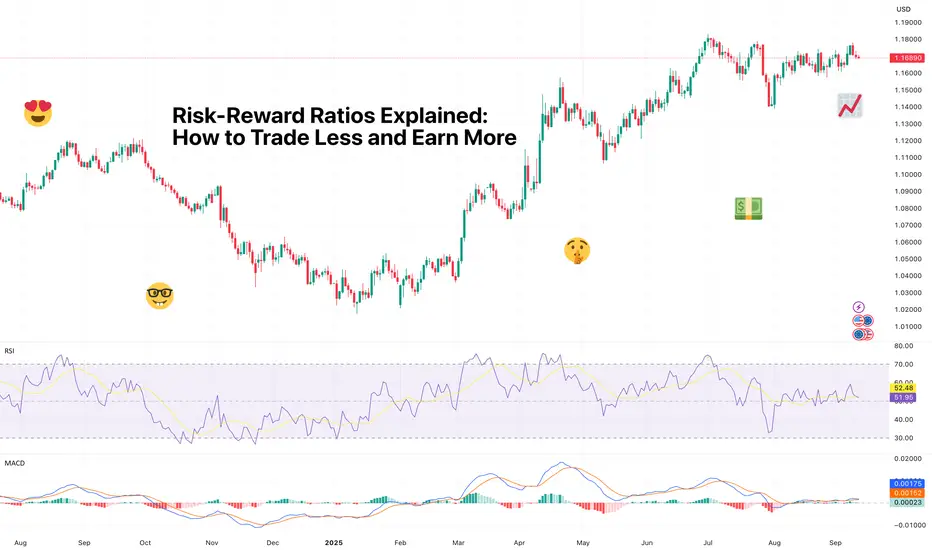
Risk-Reward Ratios Explained: How to Trade Less and Earn MoreIf you’ve been trading for a while, you’ve probably had one of those weeks where you take 15 trades, stress over every tick, barely sleep – and somehow, your P&L ends up red anyway.
Meanwhile, someone in your Discord chat casually posts their “one trade of the week” that banked more than your entire month.
The difference? They understand risk-reward ratios (unless they’re social-media influencers and have a course to sell). The ones that get risk-reward ratios right aren’t trading more, they’re trading less, better.
And that’s what we’re diving into today: how to use risk-reward to stop overtrading, focus on higher-quality setups, and finally give your capital the respect (and break) it deserves.
💡 What Risk-Reward Really Means
At its core, the risk-reward ratio (RRR) tells you how much you’re willing to lose compared to how much you aim to gain. But don’t let the simplicity fool you – mastering this concept separates the true traders from the exit liquidity.
Say you’re risking $100 to make $300. That’s a 1:3 risk-reward ratio – for every $1 on the line, you’re targeting $3 in return.
The beauty is, you don’t need to be right most of the time to make money. At a 1:3 ratio, you can lose six trades out of ten and still come out ahead. That flips the game from “I need to be right” to “I just need to manage risk.”
But, believe it or not, most traders do the opposite. They risk $300 to make $100, cut winners too early, and widen stops when trades go south. That’s not risk management; that’s donation season.
📐 Why This Isn’t Just About Math
Risk-reward ratios look clean on paper, but in real life, psychology can ruin everything.
Picture this:
You plan a beautiful 1:3 setup.
The trade starts working, you’re up 1R, and you panic.
You close early “just to lock in profits.”
If you’ve been around for a while, you’ve heard the saying “You never go broke taking profits.” True. But cutting winners early might mean missing out, hitting your goals slower or not hitting them at all.
Pro tip: once you’re up 1R, consider putting a stop at breakeven and let your take profit stay where you set it initially.
Because there’s a flip side, too. When trades go against you, emotions tell you to give it a little more room. You move your stop. Then you move it again. Suddenly, your carefully planned 1:3 trade becomes a 3:1 loser.
This is where discipline comes in. A risk-reward plan only works if you have the discipline to stick to it . Otherwise, you’re trading vibes, not setups.
🎯 The Sweet Spot for Most Traders
There’s no universal “best” ratio, but for most retail traders these setups work fine:
Day traders often aim for around 1:1 to 1:2
Swing traders typically prefer 1:3 to 1:4
Position traders can stretch to 1:5 or higher
Why? Higher timeframes give price more space to breathe. If you’re scalping, you can’t realistically aim for a 1:5 setup unless you enjoy watching charts like they’re Netflix and crying when spreads eat your edge.
But here’s where traders mess up: Instead of finding setups that naturally offer good ratios, they force them. They shrink stops to chase a flashy 1:6 RRR and end up getting wicked out by noise. Quality setups beat aggressive plays more often than not.
🚀 Asymmetric Risk-Return: The Home Run Setup
Let’s talk about asymmetric bets – trades where the upside massively outweighs the downside. Think 1:10, 1:15, or even 1:20 setups.
These are rare, but they’re game-changers when they hit.
Imagine risking $100 with a tight stop on a breakout setup. If price pops and you catch the move early, you could ride it for $1,500 or more. That’s a 15R trade – the kind that can pay for weeks, sometimes months, of smaller losses.
Here’s a recent example in FX:GBPUSD . The pair hit a double top in mid-August and immediately reversed, piercing the $1.3590 (a prior peak) by just 5 pips. Say you spotted that double-top formation and shorted with a 10-pip stop.
You’d survive the rise and then enjoy a 200-pip reward. That’s 20R in the bag, provided you exited right before the trend turned.
But here’s the trade-off:
You’ll get stopped out more often.
You need patience to let the winners actually run.
You have to accept discomfort – watching price retrace without panic-selling your position.
The market sharpshooters who master asymmetric setups don’t chase them every day. They stalk clean breakouts, major trend reversals, or high-conviction catalysts – and when the trade lines up, they size big, set a tight stop, and let the probabilities do the heavy lifting.
It’s less about being right every time and more about letting one big win offset multiple small losses.
🧩 Making Risk-Reward Work for You
Understanding ratios isn’t enough. You need a process:
Start with risk first
Decide how much you’re okay losing per trade – most pros cap it at 1–2% of account size.
Find logical stops, not emotional ones
Set stops based on structure – below support, above resistance, or at levels where your idea is simply wrong.
Set realistic targets
Don’t dream of 1:10 on a choppy Tuesday unless there’s a major catalyst to back it up.
Let math guide position sizing
Smaller stops mean larger position sizes for the same risk, but stay consistent with your capital exposure.
By planning before you enter, you flip the game from guessing to executing. That’s when risk-reward stops being theory and starts being strategy.
📈 Risk-Reward in Different Market Conditions
Markets change character, and your RRR should adapt too.
In strong trending markets , you can aim for bigger ratios since momentum carries trades further.
In range-bound conditions , scaling back to 1:1.5 or 1:2 makes sense – breakouts fail more often.
During news-heavy weeks , either widen stops or stay flat if you’re risk-averse. Chasing trades when Powell’s mic is on ? Risky business.
The smart traders bend their risk-reward ratios based on volatility instead of forcing the same plan everywhere.
🏖️ Trade Less, Profit More
Here’s the counterintuitive truth: the fewer trades you take, the more money you’ll likely make. In other words, less is more.
Focusing on high-quality setups with favorable RRRs means:
Less noise
Less overtrading
More time for actual analysis instead of gambling
You don’t need to catch every move. Stick to your RRR strategy, take care of the losses, and let profits take care of themselves.
🎯 The TradingView Edge
This is where tools make life easier:
Use Supercharts to visualize risk-reward zones before you enter.
Once inside a chart, navigate to the left-hand toolbar and spot the icon where it says Projection . Pick Long position for long risk-reward ratio, and Short position for short risk-reward ratio. Here’s a helpful tutorial in case you need some guidance.
Set alerts at key levels so you’re not glued to your screen.
Scan with screeners to find setups with volatility and structure that match your target ratios. heatmaps can help, too.
And finally, check out the newest product we launched, Fundamental Graphs , allowing you to compare plenty of metrics across multiple companies (we’re talking earnings, cash flows, net income, revenue, all that good stuff).
👉 The Takeaway
Risk-reward ratios aren’t a thing to consider – they’re a pillar of profitable trading. You don’t need to predict the market perfectly; you need to structure your trades so that your wins pay for your losses, and then some.
For most traders, the shift is simple:
Stop chasing every setup.
Start filtering for trades where the upside dwarfs the downside.
And when you get the rare asymmetric winner, ride it like your P&L depends on it – because it does.
Off to you : What’s your RRR strategy? Are you a defensive player or you’re chasing the asymmetric trades? Share your approach in the comments!
Community ideas
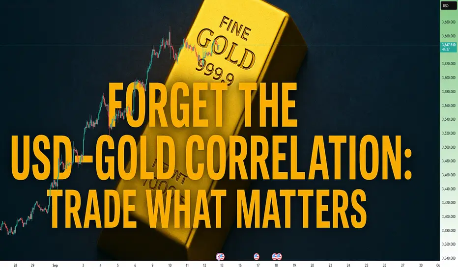
Forget the USD–Gold Correlation: Trade What MattersI took my first steps in the markets back in 2002 with stock investments. Real trading, however—the kind involving leverage, speculation, and active decision-making—began for me in 2004.
Like any responsible beginner, I started by taking courses and reading the classic trading books. One of the first lessons drilled into me was the inverse correlation between the US dollar and gold.
Fast forward more than 20 years, and for the past 15, XAUUSD has been my primary focus. And here’s the truth: I’m here to tell you that relying on USD–gold correlation is a mistake.
In this article, I’ll explain why you should avoid it, and more importantly, I’ll show you how to think like a “sophisticated” trader—especially if you can’t resist looking at the DXY .
Let’s Dissect the Myth
And for those who will say: “How on earth can you call this a mistake? Everyone knows gold moves opposite to the dollar!” — let’s dissect this step by step.
There couldn’t be a better example than 2025. We’re in the middle of a clear bullish trend in gold. Prices are climbing steadily, but not only against USD.
If gold were truly just the inverse of DXY, this overall rally wouldn’t exist. But it does. Why? Because the real driver isn’t the dollar falling — it’s demand for gold itself . Central banks are buying, funds are reallocating, and investors see gold as a store of value.
The Simple Logic That Breaks the Correlation
If it were truly a mirror correlation, then XAU/EUR would have been flat for years. Think about it: if gold only moved as the “inverse of the dollar,” then against other currencies it should show no trend at all. But the charts tell a completely different story.
Gold has been rising not just in USD terms, but also in EUR, GBP, and JPY. That means the move is not about the dollar being weak — it’s about gold being in demand.
This simple observation destroys the illusion of a strict USD–gold inverse correlation. If gold climbs across multiple currencies at the same time, the driver can’t be the dollar. The driver must be gold itself.
Why Correlation Thinking Creates Frustration
This is exactly why I tell you to ignore the so-called correlation: because it distracts you. You end up staring at the DXY when in reality, you’re trading the price of gold.
And that’s where frustration kicks in. You’re sitting on a position, watching the dollar index going higher, and you start yelling at the screen: “DXY is going up, so why isn’t gold falling? Why is my short position bleeding instead of working?”
I’ve been there many years ago, I know that feeling. But here’s the truth: gold doesn’t care about your correlation. It doesn’t care that DXY is green, red or pink. It moves on its own flows. And when you finally accept that, your trading becomes much cleaner. You stop being trapped by illusions and start focusing on the only thing that matters: the demand and supply of gold itself.
Where the Confusion Comes From
So where does all this confusion come from? Let’s take an example: imagine we get a very bad NFP number. That translates into a weaker USD. What happens? XAUUSD ticks higher.
Now, most traders immediately scream: “See? Inverse correlation!” But that’s not what’s really happening. The move you’re seeing is just a re-alignment of gold’s price in dollar terms. It’s noise, not a fundamental shift in gold’s trend.
If gold is in a downtrend overall, this kind of move doesn’t suddenly make it bullish. It’s just a temporary adjustment because the denominator (USD) weakened. On the other hand, if gold itself is already strong, such an event can act as an accelerator, pushing the trend even stronger.
The key is this: the dollar can influence the short-term pricing of XauUsd, but it doesn’t define the trend of gold. That trend is driven by demand for gold as an asset.
A Recent Example That Says It All
Let’s take a very recent example. Over the past month, DXY has been stuck in a range — no breakout, no major trend. Yet gold hasn’t just pushed higher in USD terms, it has made new all-time highs in XAU/EUR, XAU/GBP, and other currencies as well.
Why? Because gold rose. Not because the dollar fell, not because of some neat inverse chart overlay. Gold as an asset was in demand — globally, across currencies.
This is the ultimate proof that gold trades on its own flows. When buyers want gold, they don’t care whether DXY is flat, rising, or falling. They buy gold, and the charts across multiple currencies show it.
What Sophistication Really Looks Like
If you really want to be sophisticated, here’s what you do:
You see a clear bullish trend in XAUUSD. At the same time, you notice a clear bearish trend in EURUSD — which means the dollar is strong. Most traders get stuck here. Their brain short-circuits: “Wait, how can gold rise if the dollar is also strong?”
But the sophisticated trader doesn’t waste time arguing with a textbook correlation. Instead, they look for the trade that makes sense: buy XAU/EUR.
Because if gold is strong and the euro is weak, the real opportunity isn’t in fighting with DXY — it’s in positioning yourself where you can earn more. That’s not correlation thinking. That’s flow thinking.
Final Thoughts
The dollar–gold inverse correlation is a myth that refuses to die. Traders cling to it because it feels simple and safe. But real trading requires letting go of illusions and facing complexity head-on.
Gold is an independent asset. It rises and falls because of demand, not because the dollar happens to be moving the other way. Once you stop staring at DXY and start trading the flows that actually drive gold, you’ll leave frustration behind and step into sophistication.
🚀 If you still need DXY to tell you where gold is going, you’re not trading gold — you’re trading your own illusions.
Liquidity Voids: Where Price Runs Through Empty Space█ Liquidity Voids: Where Price Runs Through Empty Space
Big moves don’t just “happen”, they happen because either buyers or sellers step aside and let price run.
A liquidity void is what’s left behind when that happens: an area on the chart where price traded with very little volume, leaving a ‘hole’ in market participation.
This is not just another fair value gap. A typical FVG can form on normal volume during strong momentum. A liquidity void specifically signals a displacement under thin conditions, meaning the move was too easy, and price often comes back to check that area later.
█ What Exactly Is a Liquidity Void?
Think of the order book as a ladder of bids and asks. Normally, price moves step by step as orders fill at each level. But when there aren’t enough orders (low liquidity), price jumps levels and that jump is your void.
On a chart, it shows up as:
A large, one-directional candle with very small or no wicks overlapping neighbors.
Little or no volume relative to the move’s size (thin participation).
Price displacement that looks almost “too clean” — no hesitation, just a straight run.
These clues tell you price didn’t just move on heavy buying/selling, it moved through empty space.
⚪ Liquidity Void Detector
Use this free Liquidity Void Detector indicator to spot liquidity voids. It signals when the market makes a relatively sharp move on comparatively low volume, helping you spot these voids in real time.
█ Why Low Volume Matters
⚪ Not All Gaps Are Voids
A fair value gap can form on high participation, think of a breakout candle with heavy volume and institutional backing. That’s an accepted price move.
⚪ Voids Are Different
A liquidity void happens when the market skips prices because there was no one there to trade. It’s an inefficient move that the market often wants to revisit and “fill in” once participation returns.
⚪ Volume as the Filter
When volume is below its own average (or below a trend baseline), it tells you this wasn’t a “healthy” move, it was a thin-book displacement.
█ How Traders Use This
⚪ Mark the Zone
Draw the high and low of the candle(s) that created the void. This is your “inefficiency zone.”
⚪ Wait for the Return
Voids often act like magnets. Price often reverses and retests or fills the void, but it can just as easily slice through the zone once revisited, as thin liquidity offers little resistance.
█ What Research Show
Academic studies on price gaps find that immediate fills are rare, but the probability of fill rises over time. Downward voids (panic selling) fill faster on average than upward voids.
Crypto traders track CME Bitcoin gaps and report over 80–90% eventually get filled, but timing is unpredictable.
Volume-adjusted strategies outperform simple gap-filling because they focus on inefficient moves, not every gap. The key is filtering for thin participation.
█ Bottom Line
Liquidity voids are not just gaps, they are evidence of skipped prices under low participation.
They tell you where price moved “too easily,” leaving behind unfinished business.
Learn to filter for low-volume displacements, mark those zones, and watch how often price comes back to rebalance them. This turns a random candle into a predictive level, one that can guide your mean reversion trades or act as a support/resistance flip in trending markets.
-----------------
Disclaimer
The content provided in my scripts, indicators, ideas, algorithms, and systems is for educational and informational purposes only. It does not constitute financial advice, investment recommendations, or a solicitation to buy or sell any financial instruments. I will not accept liability for any loss or damage, including without limitation any loss of profit, which may arise directly or indirectly from the use of or reliance on such information.
All investments involve risk, and the past performance of a security, industry, sector, market, financial product, trading strategy, backtest, or individual's trading does not guarantee future results or returns. Investors are fully responsible for any investment decisions they make. Such decisions should be based solely on an evaluation of their financial circumstances, investment objectives, risk tolerance, and liquidity needs.

Understanding Elliott Wave Theory with BTC/USD If you’ve ever stared at a Bitcoin chart and thought, “ This looks like chaos ”, Ralph Nelson Elliott might disagree with you. Back in the 1930s, Elliott proposed that markets aren’t just random squiggles — they actually move in recognizable rhythms. This became known as Elliott Wave Theory .
So, what is Elliott Wave Theory? In the simplest terms, it’s the idea that market psychology unfolds in waves: five steps forward, three steps back, repeat. Not every chart follows it perfectly, but when you see it play out, it feels like spotting order in the middle of crypto madness.
⚠️ Before we dive in: remember, no single tool or pattern works alone. Elliott wave trading is most useful when combined with other methods.
The Elliott Wave Principle
At the heart of the Elliott Wave principle are two phases:
Impulse Waves (5 waves) : Markets advance in five moves — three with the trend, two counter-trend. This is when optimism snowballs.
Corrective Waves (3 waves) : The market cools off in three moves. Usually messy, choppy, and fueled by doubt.
Put them together, and you get a “5-3“ structure that repeats at different scales. That’s what gives Elliott Wave its fractal character. Again, don’t treat this as a crystal ball. Elliott Wave Theory rules are guidelines, not guarantees. Real-world Bitcoin charts bend, stretch, and sometimes ignore them altogether.
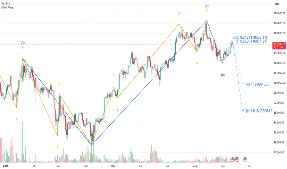
Elliott Wave Theory Explained with BTC
Let’s use an example: Bitcoin’s rally from late 2020 to early 2021 . From the breakout near $10K, BTC marched up in what could be counted as five waves: first up, a small pullback, another surge, another dip, and finally the euphoric run past $60K. Then came the correction. Summer 2021 brought a messy three-wave retrace, pulling price all the way back toward $30K before the market caught its breath.
That’s a textbook case of Bitcoin Elliott wave analysis . But notice: it wasn’t clean. Some traders counted the waves differently. Some saw extensions or truncations. That’s the thing with Elliott — interpretation matters as much as the rules.
Elliott Wave Theory Rules and Flexibility
The classic Elliott wave rules say things like: Wave 2 can’t retrace more than 100% of Wave 1. Wave 3 is never the shortest impulse wave. Wave 4 can’t overlap with Wave 1 in most cases.
But in practice, Bitcoin often blurs these lines. Extreme volatility, liquidation cascades, and macro shocks can distort wave counts. That’s why even seasoned analysts will say, “This is my Elliott count,” not the Elliott count.
The takeaway? Think of Elliott as a lens, not a lawbook.
Tools That Pair with Elliott
Many traders use the MT5 Elliott Wave Indicator or TradingView drawing tools to sketch their wave counts. Despite the waves becoming far more meaningful when tied to other signals:
Fibonacci Retracements: For example, watching how corrections line up with golden pocket levels. Momentum Oscillators: That confirm or contradict the wave structure. Macro Sentiment: Shifts that often align with corrective or impulsive phases.
Elliott Wave Theory trading doesn’t exist in a vacuum. Used alone, it’s like trying to predict the weather with just cloud shapes.
Why Beginners Should Care
If you’re new, you might be asking: “ Okay, but why bother with this at all? ” The answer: Elliott Wave Theory explained the psychology behind price swings long before the existence of cryptocurrency. It captures the human emotions behind markets — fear, greed, doubt, euphoria. And Bitcoin, perhaps more than any other asset, runs on psychology.
So whether you’re sketching waves, testing them on the Bitcoin Elliott wave chart , or just trying to understand why BTC always seems to surge then collapse, this framework helps put the chaos into context.
Final Thoughts 🌊
What is Elliott Wave Theory in trading? It’s not a magic formula. It’s a structured way of looking at markets through recurring patterns of optimism and pessimism.
And just like with every other tool we’ve discussed, it’s not about using it alone. The best insights come when you combine the Elliott Wave principle with other indicators: Fibonacci, moving averages, and even plain old support and resistance.
So the next time someone posts a “ wave count ” on a Bitcoin Elliott Wave analysis, don’t take it as gospel. Treat it as one possible map of where we are in the cycle. Because in trading, it’s never about certainty. It’s about perspective.
Risk, Psychology & Performance in Global MarketsPart 1: Risk in Global Markets
1.1 Understanding Risk
In financial terms, risk refers to the probability of losing money or failing to achieve expected returns. Global markets face multiple layers of risk, such as:
Market Risk: The risk of losses due to fluctuations in stock prices, interest rates, currencies, or commodities.
Credit Risk: The possibility that a borrower defaults on debt.
Liquidity Risk: Difficulty in buying/selling assets without affecting their price.
Operational Risk: Failures in systems, processes, or human errors.
Geopolitical Risk: Wars, sanctions, trade disputes, or policy changes.
Systemic Risk: Collapse of interconnected institutions, like the 2008 financial crisis.
Each of these risks interacts differently depending on global conditions. For instance, rising U.S. interest rates strengthen the dollar, creating ripple effects in emerging markets, where currencies may depreciate and capital outflows increase.
1.2 Measuring Risk
Several tools and models measure financial risk:
Value at Risk (VaR): Estimates the maximum potential loss over a certain period with a given confidence level.
Beta Coefficient: Measures stock volatility relative to the overall market.
Stress Testing: Simulates extreme scenarios (e.g., oil at $200 or a sudden war).
Risk-Adjusted Metrics: Like the Sharpe ratio (return vs. volatility) and Sortino ratio (downside risk).
But risk is not just statistical; it is perceived differently across regions and cultures. A European fund manager may worry about ECB monetary policy, while an Asian investor may focus on currency volatility.
1.3 Risk Management Strategies
Global investors adopt multiple approaches:
Diversification: Spreading assets across regions, sectors, and instruments.
Hedging: Using derivatives (options, futures, swaps) to limit downside.
Position Sizing: Allocating only a portion of capital per trade to limit losses.
Stop-Loss Orders: Automatic triggers to exit positions when losses exceed a threshold.
Macro Hedging: Large funds may hedge exposure to entire regions or asset classes.
An important truth: risk can be managed, but never eliminated. The 2008 financial crisis, COVID-19 crash, and Russia-Ukraine war prove that unforeseen shocks can disrupt even the most sophisticated models.
Part 2: Psychology in Global Markets
2.1 Human Behavior and Trading
While quantitative models dominate headlines, human psychology drives global markets more than numbers. Investors are emotional beings, influenced by fear, greed, hope, and regret.
This is why markets often deviate from fundamentals. During bubbles (dot-com in 2000, housing in 2008, or cryptocurrencies in 2021), prices rise far above intrinsic value due to herd mentality. Conversely, panic selling during crashes can push prices far below fair value.
2.2 Behavioral Finance Theories
Prospect Theory (Kahneman & Tversky): People fear losses more than they value equivalent gains — a $100 loss feels worse than a $100 gain feels good.
Herd Behavior: Investors follow the crowd, assuming others know better.
Overconfidence Bias: Traders overestimate their skills, leading to excessive risk-taking.
Anchoring: Relying too much on initial information, like a stock’s IPO price.
Confirmation Bias: Seeking information that supports existing beliefs while ignoring contrary evidence.
Global markets are full of such psychological traps. For example, in 2020, when oil prices went negative for the first time, many retail traders underestimated risks and held losing positions, driven by hope of a quick rebound.
2.3 Emotions in Trading
The two strongest emotions in trading are:
Fear: Leads to panic selling, hesitation, and missed opportunities.
Greed: Encourages over-leveraging, chasing trends, and holding on too long.
Successful global traders learn to master these emotions. The key is not eliminating them (which is impossible) but managing and channeling them into rational decision-making.
2.4 Psychological Challenges in Global Markets
Information Overload: With 24/7 global markets, traders face endless news, data, and rumors. Filtering is essential.
Time Zone Stress: Global traders deal with Asian, European, and U.S. sessions, often leading to fatigue.
Cultural Differences: Risk tolerance varies by region; for example, U.S. traders are often more aggressive than Japanese institutional investors.
Uncertainty Fatigue: Continuous shocks (pandemics, wars, elections) can create stress and cloud judgment.
2.5 Building Mental Strength
To succeed in global markets, traders must build psychological resilience:
Discipline: Following a trading plan and avoiding impulsive actions.
Patience: Waiting for high-probability setups instead of chasing every move.
Emotional Regulation: Techniques like meditation, journaling, or structured routines.
Learning from Losses: Viewing mistakes as tuition fees for education.
Part 3: Performance in Global Markets
3.1 Defining Performance
Performance in markets is not just about absolute profits. It involves risk-adjusted returns, consistency, and sustainability.
For example:
A trader who makes 20% with controlled risk is performing better than one who makes 40% but risks everything.
Institutions are judged by their ability to generate alpha (returns above the benchmark).
3.2 Performance Metrics
Global investors use multiple measures:
Sharpe Ratio: Return vs. volatility.
Alpha & Beta: Outperformance relative to the market.
Max Drawdown: Largest peak-to-trough loss.
Win Rate vs. Risk-Reward Ratio: High win rates are useless if losses exceed gains.
Annualized Returns: Long-term performance consistency.
3.3 Performance Drivers
Performance in global markets depends on:
Knowledge: Understanding global economics, geopolitics, and industry cycles.
Execution: Timing trades and managing entries/exits.
Technology: Use of AI, algorithms, and big data for competitive edge.
Psychological Stability: Avoiding impulsive mistakes.
Risk Management: Limiting losses to survive long enough to benefit from winners.
3.4 Institutional vs. Retail Performance
Institutional Investors: Hedge funds, sovereign wealth funds, and pension funds have resources, research, and advanced tools, but are constrained by size and regulations.
Retail Traders: More flexible and agile, but prone to overtrading and psychological traps.
Both must balance risk, psychology, and performance — though in different ways.
Conclusion
Risk, psychology, and performance are the three pillars of global market participation.
Risk reminds us that uncertainty is inevitable and must be managed wisely.
Psychology teaches us that emotions shape markets more than numbers.
Performance highlights that success lies not in short-term gains but in consistent, risk-adjusted returns.
The integration of these factors is what separates amateurs from professionals, and short-term winners from long-term survivors.
As global markets evolve with technology, geopolitics, and changing investor behavior, mastering these three elements will remain the ultimate edge for traders and investors worldwide.

Regional & Country-Specific Global Markets1. North America
United States
The U.S. is the world’s largest economy and the beating heart of global finance. It hosts the New York Stock Exchange (NYSE) and NASDAQ, two of the biggest stock exchanges globally. The U.S. dollar serves as the world’s reserve currency, making American financial markets a benchmark for global trade and investment.
Strengths:
Deep and liquid capital markets
Technological innovation hubs (Silicon Valley, Boston, Seattle)
Strong consumer demand and advanced services sector
Risks:
High national debt levels
Political polarization affecting policy stability
Trade tensions with China and other countries
Key industries include technology, healthcare, energy, defense, and finance. U.S. policies on interest rates (through the Federal Reserve) ripple across every global market.
Canada
Canada’s economy is resource-heavy, with strengths in energy (oil sands, natural gas), mining (nickel, copper, uranium), and forestry. Toronto hosts a vibrant financial sector, and Canada’s stable political environment attracts global investors.
Strengths: Natural resources, stable banking sector
Challenges: Heavy reliance on U.S. trade, vulnerability to oil price swings
Mexico
As a bridge between North and Latin America, Mexico has growing manufacturing and automotive industries, heavily integrated with U.S. supply chains (especially under USMCA trade agreement). However, crime, corruption, and political risks remain concerns.
2. Europe
Europe is home to some of the world’s oldest markets and remains a global hub for trade, technology, and finance.
European Union (EU)
The EU is the world’s largest single market, with free movement of goods, people, and capital across 27 member states. The euro is the second-most traded currency globally.
Strengths: High levels of economic integration, advanced infrastructure, strong institutions
Weaknesses: Aging population, energy dependency (especially after the Russia-Ukraine war)
Germany
Germany is the powerhouse of Europe, leading in automobiles, engineering, chemicals, and renewable energy. Frankfurt is a major financial hub.
Opportunities: Transition to green energy, high-tech industries
Risks: Export dependency, demographic challenges
France
France blends industrial strength with luxury, fashion, and tourism industries. Paris is also a growing fintech hub.
United Kingdom
Post-Brexit, the UK operates independently of the EU, but London remains a global financial center. Britain leads in finance, pharmaceuticals, and services.
Eastern Europe
Countries like Poland, Hungary, and Romania are emerging as manufacturing hubs due to lower labor costs, attracting supply chain relocations from Western Europe.
3. Asia-Pacific
Asia-Pacific is the fastest-growing region, driven by China, India, and Southeast Asia.
China
China is the world’s second-largest economy and a manufacturing superpower. It dominates global supply chains in electronics, textiles, and increasingly, electric vehicles and renewable energy.
Strengths: Huge domestic market, government-led industrial policy, global export strength
Challenges: Debt, slowing growth, geopolitical tensions with the U.S.
Markets: Shanghai Stock Exchange, Shenzhen Stock Exchange, and Hong Kong as a global financial hub
India
India is one of the fastest-growing major economies, with strong potential in IT services, pharmaceuticals, digital payments, manufacturing, and renewable energy.
Strengths: Young population, digital transformation, strong services sector
Challenges: Infrastructure gaps, unemployment, bureaucratic hurdles
Markets: NSE and BSE, with rising global investor participation
Japan
Japan has a mature economy with global leadership in automobiles, electronics, and robotics. The Tokyo Stock Exchange is one of the largest in the world.
Strengths: Advanced technology, innovation, strong corporate governance
Challenges: Aging population, deflationary pressures
South Korea
South Korea is a global leader in semiconductors (Samsung, SK Hynix), automobiles (Hyundai, Kia), and consumer electronics. The KOSPI index reflects its market vibrancy.
Southeast Asia
Countries like Vietnam, Thailand, Indonesia, and Malaysia are emerging as new growth centers, benefiting from supply chain shifts away from China.
Vietnam: Manufacturing hub for electronics and textiles
Indonesia: Rich in resources like nickel (critical for EV batteries)
Singapore: Leading global financial and logistics hub
4. Latin America
Latin America’s markets are resource-driven but often volatile due to political instability and inflation.
Brazil
The largest economy in Latin America, Brazil is a major exporter of soybeans, coffee, iron ore, and oil. It also has a growing fintech and digital economy sector.
Argentina
Argentina struggles with recurring debt crises and inflation, but it has strong potential in lithium reserves, agriculture, and energy.
Chile & Peru
Both are resource-rich, particularly in copper and lithium, making them crucial for the global clean energy transition.
Mexico
(Already covered under North America, but plays a dual role in Latin America too.)
5. Middle East
The Middle East’s economies are largely oil-driven, but diversification is underway.
Saudi Arabia
Through Vision 2030, Saudi Arabia is reducing reliance on oil by investing in tourism, renewable energy, and technology. The Tadawul exchange is gaining global importance.
United Arab Emirates (UAE)
Dubai and Abu Dhabi are major global hubs for trade, logistics, and finance. Dubai International Financial Centre (DIFC) attracts global capital.
Qatar & Kuwait
Strong in natural gas exports and sovereign wealth investments.
Israel
Israel is a “startup nation,” leading in cybersecurity, AI, fintech, and biotech. Tel Aviv has a vibrant capital market.
6. Africa
Africa is rich in natural resources but has underdeveloped capital markets. Still, its youthful population and growing middle class present opportunities.
South Africa
The most advanced African economy with a diversified market in mining, finance, and retail. The Johannesburg Stock Exchange (JSE) is the continent’s largest.
Nigeria
Africa’s largest economy, dependent on oil exports, but also growing in fintech (mobile payments, digital banking).
Kenya
A leader in mobile money innovation (M-Pesa) and a gateway to East Africa.
Egypt
Strategically located, with a mix of energy, tourism, and agriculture. Cairo plays an important role in the region’s finance.
Opportunities & Risks Across Regions
Opportunities
Emerging markets (India, Vietnam, Nigeria) offer high growth potential.
Green energy and digital transformation create cross-border investment avenues.
Regional trade blocs (EU, ASEAN, USMCA, AfCFTA) enhance integration.
Risks
Geopolitical conflicts (Russia-Ukraine, U.S.-China tensions)
Currency fluctuations and debt crises in emerging markets
Climate change disrupting agriculture and infrastructure
Inflation and interest rate volatility
Conclusion
Regional and country-specific global markets together form the backbone of the international economic system. While North America and Europe remain financial powerhouses, Asia-Pacific is the fastest-growing engine, the Middle East is transforming from oil dependency to diversification, Latin America is leveraging its resources, and Africa stands as the future growth frontier.
For investors and businesses, the key lies in understanding the unique strengths, weaknesses, and risks of each market while recognizing their global interconnectedness. The future will likely see more multipolarity—where not just the U.S. and Europe, but also China, India, and regional blocs shape the course of the global economy.

Concept of GON...Overview
Concept of GON - Get Out Now!!!
Thanks to spending most of my time on the wrong side of the markets, the GON (Get Out Now!!!) found me.
GON aids in telling me when the markets are about to gain momentum and start to move strongly against a wrong position, the realisation check to save oneself...
Understanding the trading journey; SPOT trading turned into glorified DCA (dollar cost average) trading, resulting in greed wanting to make more and then fighting this cumbersome world of liquidations, sizing, leveraging continually beaten by the markets.
Clarity on Abbreviations (how would one word it)
F8 = Fibonacci tool in short, makes it easier to withstand typos.
print ('F'+len('ibonacci'))
Last leg - The last leg is calculated from the start/beginning of the trend till the last highest high (HH) or lowest low (LL) position - dependant on direction of the trend. This last stretch/movement whereby the F8 tool is pulled/drawn from the top and bottom, in this article be referred to as the last leg.
External leg - This is the bigger move before the last leg.
Golden Pocket - between 0.618 (or 61.8%) and 0.65 (or 65%) of the last leg
Inverse Pocket - taking the opposite position of the golden pocket, calculating 100 - 61.8 (38.2) and 100 - 65 (35)
Momentum - it would be the force used to keep the price moving in one direction with little or no retracements.
Retracement value - The % mapped to the K8 tool position, this position would be compared against either the last leg or external leg.
Mixing F8 and Momentum
The F8 is useful in many ways, for me it would be to identify points of interest (POI), also putting a name to the reaction %.
During the course of learning the markets, what made sense to me about this Great F8 tool and how I could make use of it.
When drawing it, there is a starting point/value of 0 and ending point/value of 1. Depending which direction, the 0 and 1 could be swapped around and in this chart the 1 position would be at bottom and 0 at top. Knowing the potential retracement % level would be useful to calculate DCA probabilities. This is by bringing factors such as the direction, size and likelihood into equation.
The last leg helps to paint the picture of what the market is doing now. The most recent market conditions formed by the latest active key players. By observing their game and looking at it from this perspective helped me to determine the trends.
By observing the retraced % value against the last leg, a few hypothesis could be made.
1. If the F8 reaction % value increases/decreases, the force behind price is strengthening and the chart gaining momentum in a given direction, (aka: lower highs | higher lows).
2. Strength of market, as price is held to the upper bracket forcing the price higher, would indicate strong buyers. If the price is held at the lower bracket forcing price lower.
3. The opportunity to DCA decreases and later in the chart nearly impossible - depending on account balance.
4. The retraced position forms the MSS (market structure shift), or BOS (break of structure). BOS confirms strength in the current trend, while MSS warns of a possible reversal and new trend forming.
More-on F8
Reaction %, vs normal Trend Statistic Analysis, vs key entries
0% = Double tops or bottoms. Meaning, price bounced at an exact location at 0%. For beginners the Key Entry to enter the trade.
30% < or < 70% < Premium/Discount zones, momentum starts to build confirming the movement and also safe to enter the markets with SL just below the 0%.
40%/60% = Golden Pocket depending on sell/buy, or how you draw'em. You comfortable with the risk, know that these give greater results.
50% = You now need to know what you are doing...
The nice thing about momentum would be that the more people notice the new trend forming, the more likely they would jump in trying to try and catch the current move of the market and this would ultimately push the price further in any given direction.
Now unto the chart.
So, to define the early beginnings of momentum, we start observing the change in trend. The trend always starts with the lowest low (LL), or HH (highest high) depending which side the new leg is forming (opposite of the external leg). From this point we observe the next price reaction during the retrace and bounce against the last leg. We expect an increased new value, thus comparing the F8 position of the lowest low (LL) and higher low (HL) for LONG/BUY, or HH (highest high) to LH (lower high) for SHORT/SELL. Whenever a higher low (HL) or lower high (LH) is formed, we draw a new leg but interestingly the retrace % value increases as the markets keep pushing higher with force and momentum is gained.
In this chart the F8 .1 is drawn at the bottom, and .0 is positioned at the location of the last leg up, highlighting the retrace % value during a retracement.
So you want to get the maximum profit from any given trade, but that would mean that your profit margin would continue to increase. Logically, who would take 10% if they could make initially 25%? There would be a buffer, like a trailing SL but calculated differently as price increases. If the markets do hold and continue, who would rejoin and re-entering the markets again pushing the price even further.
In the world of DCA, you should have high volatility, but with leverage and sizing it becomes tricky and you perhaps "have one shot" . The outcome of this COIN reached just over 70% before retracing, and when it did retrace returned to +-2% of the original position around 25 days.
This technique may be tedious to continually draw the K8 on the last leg, especially as new higher highs or lower lows are formed, whereby one need to look at the new retrace % value and calculate if it would exceed that of the previous retrace value. Think this is where MSS and BOS would help, as it would be the same position.
If you are following the trend, you have a position working for you, then following with a SL (stop-loss) at the last formed MSS or BOS would be safe for greater profits.
If the trend isn't your friend, notice the trends shifting with momentum and be GON!!!
This isn't f inancial or trading advice, rather an interesting phenomenal aspect which helped me understand the usefulness of the F8 tool during any trade. Also do not promote any DCA strategies.
Hope that you had fun reading this article.
Wasn't myself in this particular trade, just taking a previous lesson learned from this COIN and seeing the relevance all around in the markets.
Welcome for correction, proper acronyms/abbreviations and any comments.

Gold Backing worldwidePart 1: The Origins of Gold as Money
Ancient Civilizations
Gold was used by Egyptians as early as 2600 BCE for jewelry, trade, and as a symbol of wealth.
In Mesopotamia, gold was valued as a unit of exchange in trade agreements.
Ancient Greeks and Romans minted gold coins, which spread across Europe and Asia.
Gold as Universal Acceptance
Because of its rarity, durability, and divisibility, gold became the universal standard of value across cultures. Unlike perishable goods or barter items, gold retained value and was easily transferable. This laid the foundation for gold to back economies centuries later.
Part 2: The Rise of the Gold Standard
19th Century Development
The classical gold standard emerged in the 19th century. Countries fixed their currencies to a certain amount of gold, ensuring stability in exchange rates. For example:
Britain officially adopted the gold standard in 1821.
Other major economies — Germany, France, the U.S. — followed by late 19th century.
How It Worked
Governments promised to exchange paper currency for a fixed quantity of gold.
This restrained governments from printing excessive money, keeping inflation low.
International trade was simplified because exchange rates were fixed by gold parity.
Benefits
Stability of currency.
Encouraged trade and investment.
Limited inflation due to money supply constraints.
Drawbacks
Restricted economic growth during crises.
Countries with trade deficits lost gold, forcing painful economic adjustments.
Part 3: Gold Backing in the 20th Century
World War I Disruptions
Most nations suspended the gold standard to finance military spending.
Post-war, many tried to return, but economic instability weakened confidence.
The Interwar Gold Exchange Standard
A modified version emerged in the 1920s, allowing reserve currencies (like the U.S. dollar and British pound) to be backed by gold.
This proved unstable and collapsed during the Great Depression.
Bretton Woods System (1944 – 1971)
After World War II, a new system was established at the Bretton Woods Conference.
The U.S. dollar became the anchor currency, convertible into gold at $35 per ounce.
Other currencies pegged themselves to the dollar.
This system created a gold-backed dollar world order where gold indirectly supported most global currencies.
Collapse of Gold Convertibility (1971)
In 1971, President Richard Nixon suspended gold convertibility (“Nixon Shock”).
Reasons: U.S. trade deficits, inflation, and inability to maintain gold-dollar balance.
This marked the beginning of fiat currency dominance.
Part 4: Gold’s Role in Modern Economies
Even though direct gold backing ended, gold remains vital:
1. Central Bank Reserves
Central banks worldwide hold gold as part of their foreign exchange reserves.
Provides diversification, stability, and acts as insurance against currency crises.
Major holders include the U.S., Germany, Italy, France, Russia, China, and India.
2. Store of Value & Inflation Hedge
Gold is a safe haven during economic or geopolitical crises.
Investors flock to gold when fiat currencies weaken.
3. Confidence in Currencies
Though fiat currencies are no longer backed by gold, the size of gold reserves adds credibility to a nation’s financial system.
4. Gold-Backed Financial Instruments
Exchange-traded funds (ETFs) backed by gold bullion.
Gold-backed digital currencies (such as tokenized assets on blockchain).
Part 5: Global Gold Reserves – Who Holds the Most?
According to World Gold Council data (2025 estimates):
United States: ~8,133 tonnes (largest holder, ~70% of reserves in gold).
Germany: ~3,350 tonnes.
Italy: ~2,450 tonnes.
France: ~2,435 tonnes.
Russia: ~2,300 tonnes (massively increased in past decade).
China: ~2,200 tonnes (increasing steadily to challenge U.S. dominance).
India: ~825 tonnes (also a large private gold ownership nation).
Smaller nations also hold gold as part of strategic reserves, although percentages vary.
Part 6: Regional Perspectives on Gold Backing
United States
No longer directly gold-backed, but U.S. gold reserves underpin the dollar’s strength.
Fort Knox remains symbolic of America’s monetary power.
Europe
The European Central Bank (ECB) and eurozone nations collectively hold significant gold.
Gold gives the euro credibility as a global reserve currency.
Russia
Increased gold reserves significantly to reduce dependence on the U.S. dollar amid sanctions.
Gold is a strategic geopolitical weapon.
China
Gradually building reserves to strengthen the yuan’s role in global trade.
Gold accumulation aligns with ambitions of yuan internationalization.
India
Holds large reserves at the central bank level and even larger amounts privately.
Gold plays a cultural, economic, and financial safety role.
Middle East
Gulf countries with oil wealth also diversify with gold reserves.
Some are exploring gold-backed digital currencies.
The Future of Gold Backing
Possible Scenarios
Status Quo – Fiat currencies dominate, gold remains a reserve hedge.
Partial Gold Return – Nations introduce partial gold-backing to increase trust.
Digital Gold Standard – Blockchain-based systems tied to gold reserves gain traction.
Multipolar Currency Order – Gold used more in BRICS or Asia-led alternatives to the dollar.
Likely Outcome
While a full gold standard is unlikely, gold’s role as a stabilizer and insurance policy will remain or even grow in uncertain times.
Conclusion
Gold backing has shaped global finance for centuries — from the classical gold standard to Bretton Woods and beyond. Although modern currencies are no longer directly convertible into gold, the metal continues to influence monetary policy, global reserves, and investor behavior. Central banks across the world still trust gold as the ultimate hedge against uncertainty.
In an age of rising geopolitical tensions, inflationary pressures, and digital finance, gold’s importance may even increase. Whether as part of central bank reserves, through gold-backed tokens, or as a foundation for regional trade systems, gold remains deeply woven into the fabric of the global monetary order.

The Witch Hunt Against 0.5R – A Reversed Perspective on TradingThe case for 0.5R: probability over ego
Most traders focus on 1:2 or 1:3 targets – but here I’ll show why 0.5R with ATR can be an easier, more consistent approach for many.
Till today, I’ve posted 6 trade ideas here on TradingView. All of them hit their targets. That’s a 100% winrate – all with the exact same simple structure.
(On TradingView, published Ideas cannot be edited or deleted – so these trades are shown exactly as they happened.)
Here’s a recent example where the 0.5R concept played out perfectly:
Before diving into the details, let’s first define two key terms: R and ATR.
What is “R”?
In trading, “R” = one unit of risk. It’s the amount you are willing to lose on a single trade.
If you risk $100 per trade, then:
• If the stop is hit → –1R = –$100.
• If the target is hit → +0.5R = +$50.
So when I say “0.5R target,” it simply means half the size of the risk you took.
What is ATR?
ATR = Average True Range, a measure of market volatility.
It tells us how much price typically moves during a given period.
By default, ATR is calculated from the last 14 candles – this is the standard setting most traders use.
Using ATR makes stops and targets logical, not random.
For example:
• 2 ATR stop, 1 ATR target = 0.5R
• 3 ATR stop, 1.5 ATR target = 0.5R
Both setups respect market volatility while keeping the same risk/reward structure.
The Setup in Numbers
All my trades here used exactly this approach:
• Stop: 2 ATR (sometimes 3 ATR)
• Target: 1 ATR (or 1.5 ATR)
• Risk/Reward: 0.5R
For example, with ATR = 1200:
• Stop = 2 ATR = 2400 points = –1R
• Target = 1 ATR = 1200 points = +0.5R
One green Trading Unicorn beats two reds – that’s the 0.5R logic.
That’s the foundation. Everything else – winrate, psychology, consistency – builds on this.
The Dogma of 1:2R, 1:3R and Higher
The trading world has developed a kind of witch hunt against any setup below 1:2 or 1:3. It has become the so-called “professional standard.”
But here’s the truth nobody talks about:
• 1:3 rarely hits on the first attempt.
• It usually takes multiple tries – each one adding risk, losses, and stress.
• By the time one 1:3 target is finally hit, many traders have already lost money or burned mental energy.
On paper, high-R multiples look perfect.
In practice, for most traders, they are psychological torture.
One small green Trading Unicorn win is often worth more than chasing oversized targets that almost never arrive.
Visual breakdown:
• 1:3 R/R – great if it hits, but usually doesn’t on the first try.
• 1:2 R/R – “more realistic,” yet still often fails before reaching target.
• 0.5R ATR – smaller, faster, higher probability – it usually hits first.
Why 0.5R Flips the Script
A 0.5R setup often looks “too small” to many traders – but that’s exactly the point.
• High probability: most trades hit target on the first attempt.
• Not mentally exhausting: no long waiting, no constant pressure.
• Quick wins and confidence: reward comes fast, reinforcing discipline.
• Consistency: with an 80%+ winrate, just a couple winners cover the losses.
Example: If 1 trade loses (–1R), only 2 winners (+2 × 0.5R = +1R) are enough to breakeven.
This isn’t just math – it’s where probability and psychology align in practice.
And here’s the hidden edge: with smaller, faster ATR-based targets, you don’t need to commit to being a “bull” or a “bear.”
• Bulls chase big breakouts, but often wait too long.
• Bears fight the trend, but usually get stopped before reversal.
• With 0.5R, you don’t need to predict who’s right. You can profit both ways, even against the trend, because the distance to target is short and realistic.
And here’s an extra advantage most traders ignore: markets range about 70% of the time and trend only 30%.
That means setups that require huge trending moves (1:2, 1:3, etc.) automatically have fewer chances.
A 0.5R setup, however, thrives in both conditions – ranging or trending – giving you far more opportunities simply because your target is closer and hits faster.
The Trading Unicorn stands in the middle, keeping both bull and bear under control – that’s the real power of the 0.5R concept.
Leverage and the “Close Target Paradox”
Many dismiss 0.5R targets as “not worth it” because they look close on the chart.
But here’s the paradox:
• Thanks to leverage, even a small target can equal meaningful percentage gains.
• On a 10k account, 1% = $100. That can be made in a few minutes – sometimes seconds – with a single 0.5R trade.
• Whether the market is quiet or volatile, the math still works.
This means you don’t need to wait for “the perfect market.”
With ATR-based sizing and proper leverage, the 0.5R concept can be applied to crypto, metals, forex, or stocks – anytime, anywhere.
Strategy in Action
For me, the 0.5R system works best in:
• Quick breakouts
• Break of structure followed by a pullback to a key level
• Confluences stacking at support/resistance
• Then targeting a 1 ATR move out of that zone
It doesn’t matter if I trade 1m charts, 1h, or 4h. The principle is the same.
Here’s another recent trade hitting target:
The Psychological Trap
But let’s be real. This strategy has a dangerous side: it’s too tempting.
• If you can make 1% in 3 minutes, your brain immediately wants to repeat it.
• “Just one more quick trade” becomes the thought that destroys consistency.
• Survival instinct takes over. Ego wants more.
• Soon, rules are broken.
This is why discipline and rules are non-negotiable.
And why, many times, a mentor is necessary – to keep us from breaking our own system for the hope of more gains.
The Wine Analogy
Think of 0.5R like a glass of wine:
• One or two? It relaxes you, maybe even healthy.
• Ten glasses? You lose control, do things you regret.
The concept itself is not dangerous.
The problem is how you use it. With moderation and rules, it becomes a consistent tool. Without them, it can become self-destruction.
The Hidden Cost of Chasing Big R
Trading is not just about money. It’s also about emotional capital.
• Every missed big-R target eats away at confidence.
• Every time you intervene because you “couldn’t hold,” you reinforce bad habits.
• Eventually, you’re not just losing money – you’re losing trust in yourself.
This is why so many traders sabotage themselves. The targets they set are beyond their psychological tolerance.
AI sanity-check (do it yourself)
You don’t have to take my word for it. Anyone with an AI in their pocket can sanity-check this:
Inputs:
• Winrate: 80%+
• Outcomes (in R): +0.5R on wins, –1R on losses
• Risk per trade: 1% of current equity (compounded)
• Pace: max 4 trades/day
• Sample size: 100–1000 trades
• Market: BTCUSD, 1-minute
• Profiles: (A) 2 ATR stop / 1 ATR target, (B) 3 ATR stop / 1.5 ATR target
• Entry filter: only confluences & high-probability breakouts
• Include: compounding
Prompt to any AI:
“Run a Monte Carlo with the above inputs and return the median equity curve, drawdown distribution, and percentiles.”
Final Thoughts
The 0.5R ATR system is not a holy grail.
But it challenges the dogma of chasing huge R multiples at all costs.
• It shows that winrate × probability can be just as powerful as high reward multiples.
• It adapts across instruments, timeframes, and lifestyles.
• It doesn’t care about ego. It cares about results.
Trading is personal. For some, 1:3 works.
For others, 0.5R unlocks the consistency they’ve been searching for.
Don’t be the elephant trying to climb a tree just because everyone else says it’s “the way.” Find what works for you.
Hope this perspective gave you some value.
Cheers,
Trading Unicorn

What Is Systematic Risk and How May It Affect Markets?What Is Systematic Risk and How May It Affect Markets?
Systematic risk affects all traders, no matter the strategy or asset class. It comes from market-wide forces—like interest rates, inflation, or geopolitical shifts—that influence entire sectors at once. Unlike unsystematic risk, it can’t be avoided through diversification. This article breaks down what systematic risk is, how it’s measured, and how traders may incorporate it into their analysis.
What Is Systematic Risk?
Systematic risk refers to the kind of risk that affects entire markets or economies, rather than just individual assets. It’s the result of large-scale forces—like inflation, interest rates, central bank policy, geopolitical conflict, or economic slowdowns—that ripple through multiple asset classes at once.
A sharp rise in interest rates, for example, tends to push bond prices lower and can drag down equity valuations as borrowing costs climb and consumer spending slows. Similarly, during a global event like the 2008 financial crisis or the COVID-19 shock in 2020, almost all sectors saw simultaneous drawdowns. These events weren’t tied to poor management or bad earnings reports—they were macro-level shifts that hit everything.
Because it’s a largely undiversifiable risk, systematic risk is a key consideration for traders assessing overall market exposure. It often drives correlation between assets, particularly in times of stress. This is why equities, commodities, and even currencies can start to move in the same direction during periods of heightened volatility.
So, can systematic risk be diversified against? Only relatively speaking. Traders and investors may shift into defensive positions to limit potential drawdowns (e.g. gold, bonds, healthcare stocks vs tech companies). However, no matter how diversified a portfolio is, it remains exposed to this kind of risk because it’s tied to broader market movements rather than asset-specific events.
Note: systematic risk differs from systemic risk. The systemic risk definition relates to the potential collapse of the financial system, such as in a banking crisis. It is rare but severe.
Systematic vs Unsystematic Risk
Systematic risk is broad and market-driven. Unsystematic risk, on the other hand, is specific to a company or sector. It might come from a product failure, a major lawsuit, or a change in management. For example, if a tech company misses earnings due to poor execution, that’s unsystematic. If the entire sector drops because of a global chip shortage or policy change, that’s systematic.
Unsystematic risk can be reduced through diversification. Holding assets across industries may help spread exposure to isolated events. But systematic risk can’t be avoided by simply adding more assets. It affects everything to some extent.
That’s why traders track both systematic and unsystematic risk—understanding where their risk is concentrated and whether their exposure is tied to broad market movements or individual events. Clear separation of the two may help traders analyse potential drawdowns more accurately.
Key Drivers of Systematic Risk
Systematic risks tend to stem from structural or macroeconomic forces, and while they can’t be avoided, traders can track them to better understand the environment they’re operating in. Below are some of the most common types of systematic risk and how they influence market-wide movement.
Monetary Policy
Central banks play a huge role in shaping market conditions. When interest rates rise, borrowing becomes more expensive, which tends to slow down spending and investment. That usually puts downward pressure on risk assets like equities. Conversely, rate cuts or quantitative easing often lead to a surge in asset prices as liquidity improves.
Traders closely monitor central bank statements and economic projections, especially from institutions like the Federal Reserve, the Bank of England, and the European Central Bank.
Inflation and Deflation
Inflation affects everything from consumer behaviour to corporate earnings. Higher inflation can reduce real returns and push central banks to tighten policy. Deflation, though less common, signals weak demand and falling prices, which also tends to hurt equities. Commodities, currencies, and bonds often react sharply to inflation data.
Economic Cycles
Booms and busts are among the most well-known examples of systematic risk, influencing everything from job creation to earnings growth. During expansions, risk appetite tends to rise. In downturns, investors often shift towards defensive assets or cash. GDP figures, manufacturing data, and consumer spending are key indicators traders watch.
Geopolitical Risk
Elections, wars, trade tensions, and sanctions can drive sharp market reactions. These events introduce uncertainty, increase volatility, and can disrupt global supply chains or investor sentiment.
Market Sentiment and Liquidity
Panic selling or sudden shifts in positioning can cause assets to move together, even if fundamentals don’t support it. During liquidity crunches, correlations spike and markets can move sharply on little news. This is often driven by leveraged positioning unwinding or large institutions adjusting risk.
Measuring Systematic Risk
Systematic risk can’t be removed, but it can be measured, and that may help traders understand how exposed they are to broader market swings.
One of the most widely used tools is beta. Beta shows how much an asset moves relative to a benchmark index. A beta of 1 indicates that the asset typically moves in the same direction and by a similar percentage as the overall market. Above 1 means it’s more volatile than the market; below 1 means it’s less volatile. For example, a high-growth stock with a beta of 1.5 would typically move 15% when the market moves 10%.
Another approach is Value at Risk (VaR), which estimates the potential loss on a portfolio under normal market conditions over a specific timeframe. It doesn’t isolate systematic risk but gives a sense of how exposed the overall portfolio is.
Traders also watch the VIX—often called the “fear index”—which tracks expected volatility in the S&P 500. When it spikes, it usually signals rising market-wide risk.
More complex models like the Capital Asset Pricing Model (CAPM) use beta and expected market returns to price risk, but some traders use these tools to get a clearer picture of how exposed they may be to movements they can’t control.
How Traders May Use Systematic Risk in Analysis
Systematic risk isn’t just a background concern—it plays a direct role in how traders assess the market, structure portfolios, and manage exposure. By understanding how market-wide forces are likely to affect asset prices, traders can adjust their approach to reflect broader conditions rather than just focusing on technical analysis or individual names.
Position Sizing and Exposure
When systematic risk is elevated—during tightening cycles, political unrest, or global economic slowdowns—traders may scale back position sizes or reduce leverage. The aim is to avoid being caught in a correlated sell-off where multiple positions move against them at once. It's common to see increased cash holdings or a shift towards lower beta assets in these periods.
Asset Allocation Adjustments
Systematic risk also shapes how capital is distributed across asset classes. For example, during periods of strong economic growth, traders may lean into equities, particularly cyclical sectors. In contrast, during uncertain or contractionary periods, there may be a move towards defensive sectors, fixed income, or commodities like gold. Some rotate between assets based on macro trends to stay aligned with the dominant forces driving markets.
Macro Analysis and Scenario Planning
Understanding systematic risks may help traders prepare for potential market reactions. A trader can analyse upcoming interest rate decisions, inflation prints, or geopolitical tensions and assess which assets are likely to be most sensitive. If recession risk increases, they may expect higher equity volatility and reassess exposure accordingly.
Correlation Tracking
As systematic risk rises, correlations between assets often increase. Traders who normally count on diversification may find their positions moving together. Keeping track of these shifts may help reduce false confidence in portfolio structure and encourage more dynamic risk controls.
Systematic Risk: Considerations
As mentioned above, systematic risk is mostly unpredictable and fully unavoidable. There are some other things you should consider when trying to analyse it. Here are a few points traders often keep in mind:
- Lagging indicators: Metrics like GDP or inflation are backwards-looking. Markets often react before the data confirms the trend.
- False signals: Beta, VaR, and the VIX can be useful, but they’re not foolproof. A low VIX doesn’t guarantee calm markets, and beta doesn’t account for real market conditions.
- Uncertainty around timing: Even if the presence of risk is clear, the timing and severity of its impact are hard to analyse with precision.
- Overreaction risk: Markets can price in fear quickly, and traders may misjudge whether a reaction is justified or temporary.
- Diversification assumptions: Assets that usually behave differently may move in sync during stress. Risk models can underestimate this.
The Bottom Line
Systematic risk is unavoidable, but understanding how it moves through markets may support traders in making decisions. By tracking macro drivers and adjusting positions accordingly, traders may respond with more clarity during volatile periods. However, it is important to take into account all the difficulties that systematic risk brings.
FAQ
What Is Systematic Risk?
Systematic risk refers to the type of risk that affects an entire market or economy. It’s driven by macroeconomic forces such as interest rates, inflation, economic health, and geopolitical events. Because it impacts broad segments of the market, systematic risk cannot be eliminated through diversification.
What Is Systematic Risk vs Unsystematic Risk?
Systematic risk is market-wide and linked to broader economic conditions. Unsystematic risk is asset-specific and tied to events like company earnings, leadership changes, or industry developments. According to theory, unsystematic risk can be reduced by holding a diversified portfolio, while systematic risk remains even with strong diversification.
What Are the Five Systematic Risks?
The main categories include interest rate risk, inflation risk, economic cycle risk, geopolitical risk, and currency or exchange rate risk. Each can affect multiple asset classes and contribute to broad market shifts.
Can You Diversify Systematic Risk?
No. While diversification may help reduce unsystematic risk, systematic risk affects most assets. It might be managed, not avoided.
This article represents the opinion of the Companies operating under the FXOpen brand only. It is not to be construed as an offer, solicitation, or recommendation with respect to products and services provided by the Companies operating under the FXOpen brand, nor is it to be considered financial advice.

What you do before a trade mattersTo succeed in trading, you need to place yourself in an optimal state as often as possible. It’s not just about the trade itself – it’s about what you do before. Your preparation is what determines how stable and effective you’ll be when it truly counts.
Of course, we can make profits even when we’re not at our best. But the risk is that we start acting in ways that don’t align with our strategy, our process, or our optimal performance. And that builds shaky foundations. For long-term success, you need something stronger.
Here are a few key things to focus on before you enter a trade:
🔋 Recharge your batteries
Trading demands energy and presence. Make sure you’ve filled up your resources before the market opens. Did you get enough sleep? Have you moved your body, worked out, or gotten fresh air? Are you taking breaks to let your brain recover? The more rested and energized you are, the sharper your decisions will be.
⏰ Decide WHEN to trade
Be honest with yourself – when do you perform at your best? Are you sharpest in the morning, or do you focus better later in the day? Do you notice yourself taking risky trades in the evening? Observe your own patterns and schedule your trading during the hours when you’re at your peak.
🚪 Shut out the noise
When you’re in a trade, your full attention needs to be there. Look at what’s stealing your focus. Maybe you should avoid reading chats or forums right before taking action. Do you have an environment where you can sit undisturbed and fully focused? Create the conditions for presence.
🧠 Got other things on your mind? Skip trading
Life always seeps into trading. If something has happened – maybe worry, conflict, or emotional turbulence – it will follow you to the screen. In those moments, it’s often wiser to pause, take care of what’s going on, and return to trading when you feel stable and clear.
Creating an optimal state means viewing trading as a whole – something that spans the entire day, not just the moments you click buy or sell. How you take care of yourself beforehand directly impacts your endurance, focus, and emotional balance.
💡 Pro Tip:
Start observing when you perform at your best. Is it morning or afternoon? Certain days of the week? Collect data on what truly makes a difference – then try to prioritize trading during those times.
Happy compassionate trading! 💙
/ Tina the Trading Psychologist

How to Close a Losing Trade?Cutting losses is an art, and a losing trader is an artist.
Closing a losing position is an important skill in risk management. When you are in a losing trade, you need to know when to get out and accept the loss. In theory, cutting losses and keeping your losses small is a simple concept, but in practice, it is an art. Here are ten things you need to consider when closing a losing position.
1. Don't trade without a stop-loss strategy. You must know where you will exit before you enter an order.
2. Stop-losses should be placed outside the normal range of price action at a level that could signal that your trading view is wrong.
3. Some traders set stop-losses as a percentage, such as if they are trying to make a profit of +12% on stock trades, they set a stop-loss when the stock falls -4% to create a TP/SL ratio of 3:1.
4. Other traders use time-based stop-losses, if the trade falls but never hits the stop-loss level or reaches the profit target in a set time frame, they will only exit the trade due to no trend and go look for better opportunities.
5. Many traders will exit a trade when they see the market has a spike, even if the price has not hit the stop-loss level.
6. In long-term trend trading, stop-losses must be wide enough to capture a real long-term trend without being stopped out early by noise signals. This is where long-term moving averages such as the 200-day and moving average crossover signals are used to have a wider stop-loss. It is important to have smaller position sizes on potentially more volatile trades and high risk price action.
7. You are trading to make money, not to lose money. Just holding and hoping your losing trades will come back to even so you can exit at breakeven is one of the worst plans.
8. The worst reason to sell a losing position is because of emotion or stress, a trader should always have a rational and quantitative reason to exit a losing trade. If the stop-loss is too tight, you may be shaken out and every trade will easily become a small loss. You have to give trades enough room to develop.
9. Always exit the position when the maximum allowable percentage of your trading capital is lost. Setting your maximum allowable loss percentage at 1% to 2% of your total trading capital based on your stop-loss and position size will reduce the risk of account blowouts and keep your drawdowns small.
10. The basic art of selling a losing trade is knowing the difference between normal volatility and a trend-changing price change.

Role of SWIFT in Cross-Border Payments1. The Origins of SWIFT
1.1 The Pre-SWIFT Era
Before SWIFT, banks relied heavily on telex messages to transmit payment instructions. Telex systems were slow, error-prone, lacked standardized formats, and required human intervention to decode and re-key messages. This often resulted in delays, fraud, and disputes in cross-border settlements.
By the early 1970s, with international trade booming, the shortcomings of telex became unsustainable. Leading banks realized the need for a global, standardized, automated, and secure communication system.
1.2 Founding of SWIFT
In 1973, 239 banks from 15 countries established SWIFT as a cooperative society headquartered in Brussels, Belgium. The goal was to build a shared platform for financial messaging, independent of any single nation or commercial entity. By 1977, SWIFT was operational with 518 member institutions across 22 countries.
2. What SWIFT Does
2.1 Messaging, Not Money Movement
A common misconception is that SWIFT transfers money. In reality, SWIFT does not hold funds, settle payments, or maintain accounts for members. Instead, it provides a standardized and secure messaging system that allows banks to communicate financial instructions such as:
Cross-border payments
Securities transactions
Treasury deals
Trade finance documents
2.2 SWIFT Message Types
SWIFT messages follow standardized formats known as MT (Message Type) series. For instance:
MT103 – Single customer credit transfer (used for cross-border payments)
MT202 – General financial institution transfer
MT799 – Free-format message (often used in trade finance)
In recent years, SWIFT has transitioned to ISO 20022, an XML-based messaging standard that provides richer data, improving compliance, transparency, and automation.
2.3 Secure Network Infrastructure
SWIFT operates through a secure, private IP-based network known as SWIFTNet, supported by data centers in Europe, the U.S., and Asia. Messages are encrypted, authenticated, and routed through SWIFT’s infrastructure to ensure confidentiality, integrity, and availability.
3. Role of SWIFT in Cross-Border Payments
3.1 Standardization of Payment Messages
One of SWIFT’s biggest contributions is standardization. By creating globally accepted message formats, SWIFT eliminates ambiguity in payment instructions. This reduces operational risks, errors, and disputes. For example, an MT103 message is universally understood by banks in over 200 countries.
3.2 Speed and Efficiency
Before SWIFT, payments could take days or even weeks to process. With SWIFT, instructions are transmitted instantly across borders. While actual settlement still depends on correspondent banking arrangements, messaging delays have been nearly eliminated.
3.3 Security and Trust
Cross-border transactions involve huge sums of money, often in the billions. SWIFT provides strong encryption, authentication, and anti-fraud protocols, making it the most trusted network for international payments.
3.4 Connectivity in Global Trade
SWIFT connects over 11,000 financial institutions in more than 200 countries and territories. This global reach makes it the backbone of cross-border trade, enabling corporates, banks, and governments to transact seamlessly.
3.5 Correspondent Banking and SWIFT
Cross-border payments usually require multiple intermediaries (correspondent banks) when two banks don’t have a direct relationship. SWIFT facilitates this process by transmitting messages along the chain of correspondent banks, ensuring funds are eventually credited to the beneficiary.
4. SWIFT in Action: An Example
Imagine a customer in India sending $10,000 to a supplier in Germany.
The Indian customer instructs their bank to transfer the funds.
The Indian bank creates an MT103 message via SWIFT, directing its correspondent bank in Europe to debit its account and credit the German bank.
The German bank receives the SWIFT message and credits the supplier’s account.
The supplier receives funds, while SWIFT has acted only as the messaging medium.
This standardized, secure communication ensures accuracy, speed, and reliability.
5. SWIFT’s Economic and Geopolitical Importance
5.1 Enabler of Globalization
SWIFT underpins international trade by making payments predictable and efficient. Without it, global supply chains, remittances, and investment flows would be significantly slower and riskier.
5.2 Role in Sanctions and Geopolitics
Because of its centrality, SWIFT has become a geopolitical tool. For instance, Iranian banks were cut off from SWIFT in 2012 and again in 2018, severely restricting Iran’s access to global markets. Similarly, Russian banks faced SWIFT restrictions in 2022 after the Ukraine invasion.
5.3 Dependence and Alternatives
The reliance on SWIFT has raised concerns about overdependence. Some countries have developed alternatives:
CIPS (China’s Cross-Border Interbank Payment System)
SPFS (Russia’s System for Transfer of Financial Messages)
UPI-based cross-border initiatives (India)
Still, SWIFT remains the dominant system due to its network effects and global acceptance.
6. Evolution and Innovations in SWIFT
6.1 SWIFT gpi (Global Payments Innovation)
Launched in 2017, SWIFT gpi transformed cross-border payments by introducing:
End-to-end tracking (like a parcel tracking system for money)
Same-day use of funds in many cases
Transparency in fees and FX rates
Confirmation of credit to beneficiary
Today, gpi covers over 80% of SWIFT cross-border traffic, making payments faster, cheaper, and more transparent.
6.2 ISO 20022 Migration
SWIFT is migrating from legacy MT messages to ISO 20022 by 2025. This shift will enable:
Richer data for compliance (e.g., sanctions screening, AML checks)
Better automation and reconciliation
Interoperability with domestic real-time payment systems
6.3 Future Technologies
SWIFT is also experimenting with blockchain, central bank digital currencies (CBDCs), and tokenized assets. For instance, SWIFT has piloted experiments linking CBDCs across different countries, positioning itself as a neutral connector even in a digital currency world.
7. Challenges Facing SWIFT
7.1 Competition from Alternatives
Regional systems like China’s CIPS or blockchain-based solutions like RippleNet challenge SWIFT’s dominance. Fintech innovations promise faster, cheaper transfers without multiple intermediaries.
7.2 Costs and Fees
While SWIFT is efficient, cross-border payments often remain costly due to correspondent bank charges. Fintech challengers are pushing for lower-cost solutions.
7.3 Cybersecurity Risks
Being the backbone of global payments, SWIFT is a prime cyber target. Incidents like the 2016 Bangladesh Bank hack, where hackers exploited SWIFT credentials to steal $81 million, highlight vulnerabilities. SWIFT responded with its Customer Security Programme (CSP) to strengthen defenses.
7.4 Geopolitical Pressures
SWIFT’s role in sanctions makes it politically sensitive. Its neutrality is constantly tested as major powers use access to SWIFT as leverage in global disputes.
8. The Future of Cross-Border Payments and SWIFT
8.1 Towards Instant Payments
Global efforts are underway to make cross-border payments as fast as domestic transfers. SWIFT is adapting by linking with real-time domestic systems and enhancing gpi.
8.2 Digital Currencies and Blockchain
The rise of CBDCs, stablecoins, and blockchain networks may disrupt SWIFT’s role. However, SWIFT’s vast network gives it an edge to act as an interoperability layer, connecting legacy systems with digital currencies.
8.3 Regulatory Harmonization
Cross-border payments face compliance challenges (AML, KYC, sanctions). SWIFT’s data-rich ISO 20022 messages can help improve regulatory oversight while maintaining efficiency.
8.4 Balancing Neutrality and Politics
SWIFT’s survival depends on maintaining neutrality while navigating political pressures. Its governance as a cooperative helps, but geopolitical rivalries may accelerate regional alternatives.
9. Conclusion
For over four decades, SWIFT has been the invisible backbone of cross-border payments. By providing a standardized, secure, and reliable messaging system, it has enabled globalization, facilitated trillions in trade and finance, and connected thousands of institutions worldwide.
Its contributions include:
Standardization of payment messages
Enhanced speed, security, and reliability
Support for correspondent banking
Enabling sanctions enforcement and geopolitical leverage
Constant evolution through SWIFT gpi and ISO 20022
Yet, challenges loom: fintech disruptions, geopolitical tensions, cybersecurity risks, and the rise of digital currencies. SWIFT’s ability to innovate and maintain global trust will determine whether it remains the nerve center of international payments in the digital era.
In summary, while SWIFT does not move money directly, its role as the messenger of global finance is irreplaceable—at least for now. The future of cross-border payments may involve blockchain, CBDCs, or regional systems, but SWIFT’s global reach, trust, and adaptability ensure that it will continue to play a central role in shaping how money flows across borders.
Balance of Payments & World Trade ImbalancesPart I: Understanding the Balance of Payments
1. What is the Balance of Payments?
The Balance of Payments is a systematic record of all economic transactions between residents of a country and the rest of the world. It includes trade in goods and services, cross-border investments, transfers, and monetary flows.
In principle, the BoP always balances: total credits (money coming in) equal total debits (money going out). However, the composition of transactions—whether surpluses or deficits in certain accounts—matters for economic stability.
2. Main Components of BoP
a) Current Account
The current account records trade in goods, services, primary income (investment income, wages), and secondary income (remittances, foreign aid).
Trade balance: Exports minus imports of goods.
Services balance: Exports minus imports of services such as tourism, IT outsourcing, shipping, etc.
Primary income: Interest, dividends, wages.
Secondary income: Transfers like remittances, pensions, grants.
A current account surplus means a country is a net lender to the rest of the world, while a deficit means it is a net borrower.
b) Capital Account
This is usually small and records transfers of capital assets, debt forgiveness, and non-produced, non-financial assets (like patents or natural resource rights).
c) Financial Account
The financial account tracks cross-border investments:
Foreign Direct Investment (FDI): Long-term investments in businesses abroad.
Portfolio Investment: Stocks, bonds, and securities.
Other Investments: Loans, trade credits, banking flows.
Reserve Assets: Central bank reserves (foreign currencies, gold, IMF position).
d) Errors & Omissions
Statistical discrepancies that arise due to imperfect data reporting.
3. Why is BoP Important?
Macro stability indicator: Reveals structural strengths/weaknesses in a country’s economy.
Policy formulation: Helps governments decide on fiscal, monetary, and trade policies.
Investor confidence: Influences credit ratings, exchange rates, and capital inflows.
Global coordination: Used by IMF, WTO, and G20 to monitor systemic risks.
Part II: World Trade Imbalances
1. Defining Trade Imbalances
A trade imbalance occurs when a country persistently runs a trade surplus (exports > imports) or trade deficit (imports > exports). While short-term imbalances are natural, structural and persistent gaps can destabilize the world economy.
2. Causes of Trade Imbalances
a) Differences in Productivity and Competitiveness
Countries with higher productivity (e.g., Germany, Japan) tend to export more, creating surpluses.
b) Currency Valuations
If a country’s currency is undervalued (e.g., Chinese yuan in the 2000s), its exports become cheaper, widening surpluses. Conversely, overvalued currencies contribute to deficits.
c) Consumption and Savings Behavior
The U.S. model: High consumption, low savings → trade deficits.
The Asian model: High savings, export-oriented growth → trade surpluses.
d) Resource Dependence
Oil-exporting nations like Saudi Arabia often run surpluses due to high energy demand.
e) Global Supply Chains
Multinational corporations fragment production globally. Goods may be “assembled in China” but use inputs from multiple countries, complicating trade balance measurement.
f) Government Policies
Subsidies, tariffs, currency interventions, and trade agreements influence competitiveness.
3. Consequences of Trade Imbalances
a) For Deficit Countries
Rising external debt.
Dependence on foreign capital.
Currency depreciation risk.
Political vulnerability (e.g., U.S.–China tensions).
b) For Surplus Countries
Overreliance on external demand.
Domestic underconsumption.
Exposure to global downturns.
Accusations of “unfair trade practices.”
c) Global Impact
Exchange rate misalignments.
Risk of trade wars and protectionism.
Global financial crises (imbalances partly fueled 2008).
Distorted capital flows—surpluses recycled into deficit-country debt markets.
Part III: Historical & Contemporary Case Studies
1. The U.S. Trade Deficit
Since the 1980s, the U.S. has run persistent current account deficits.
Driven by high consumption, dollar reserve currency status, and globalization.
Funded by foreign purchases of U.S. Treasury bonds, especially by China and Japan.
2. China’s Surplus
Export-led industrialization strategy.
Massive trade surpluses in the 2000s, peaking near 10% of GDP in 2007.
Accumulated trillions in foreign reserves.
Gradual rebalancing after 2010, but surplus remains large.
3. Eurozone Imbalances
Germany runs huge surpluses, while southern Europe (Greece, Spain, Italy) historically ran deficits.
Imbalances within a common currency area created debt crises during the 2010 Eurozone crisis.
4. Oil Exporters
OPEC countries run surpluses during high oil prices.
But face volatility when prices crash.
5. Japan
Historically a surplus country due to its manufacturing strength.
Demographic decline now affecting its external balance.
Part IV: Policy Responses to Trade Imbalances
1. Domestic Policy Options
For deficit countries: Promote exports, encourage savings, reduce fiscal deficits.
For surplus countries: Stimulate domestic consumption, allow currency appreciation.
2. Exchange Rate Adjustments
Flexible exchange rates can correct imbalances, but in practice, many governments intervene in currency markets.
3. Trade Agreements & Protectionism
Tariffs, quotas, and trade deals aim to adjust trade balances, though they often create new distortions.
4. Role of International Institutions
IMF: Provides surveillance, loans, and adjustment programs.
WTO: Mediates trade disputes.
G20: Coordinates global responses to imbalances.
Part V: Future Outlook
1. Digital Economy & Services Trade
The rise of digital platforms, e-commerce, and remote services (IT, finance, design) is reshaping BoP structures. Countries strong in digital services (India, U.S., Ireland) may offset merchandise deficits.
2. Geopolitical Shifts
U.S.–China rivalry, reshoring, and supply chain diversification will affect trade balances.
3. Climate Transition
Green technologies, carbon tariffs, and energy transitions will change global trade patterns. Oil exporters may see reduced surpluses in the long term.
4. Multipolar Currencies
The U.S. dollar may gradually lose dominance, with the euro, yuan, and digital currencies playing larger roles in financial accounts.
5. AI & Automation
Advanced technology may reduce labor-cost advantages, altering comparative advantage and global imbalances.
Conclusion
The Balance of Payments is not just a technical accounting statement—it is a powerful lens through which to view the global economy. Persistent world trade imbalances reflect deep structural factors: consumption patterns, savings rates, productivity, resource endowments, and government strategies.
While deficits and surpluses are not inherently “bad,” their persistence at extreme levels poses risks of instability, inequality, and geopolitical friction. Addressing them requires coordinated domestic reforms, international policy cooperation, and adaptive strategies for a rapidly changing world economy.
In the 21st century, as global trade evolves with digitalization, climate change, and shifting geopolitics, the challenge will be to ensure that the Balance of Payments reflects not just imbalances, but sustainable, inclusive, and resilient patterns of global economic exchange.

Role of G7 and G20 in World Markets1. Historical Background
1.1 Origins of the G7
The G7 originated in the 1970s oil crisis and currency instability. The breakdown of the Bretton Woods system (1971) and the 1973 oil shock forced leaders of the US, UK, France, West Germany, Italy, and Japan to coordinate policies.
The first meeting took place in 1975 at Rambouillet, France. Canada joined in 1976, making it the G7.
The forum was designed as an informal space for dialogue among advanced economies, free from the rigid bureaucracy of the IMF or UN.
1.2 Expansion into G20
By the late 1990s, globalization had empowered emerging markets like China, India, Brazil, and South Africa.
The Asian Financial Crisis of 1997–98 exposed the limitations of the G7, which could not represent the interests of developing nations.
The G20 was created in 1999, initially as a forum for finance ministers and central bank governors.
Following the 2008 Global Financial Crisis, the G20 was elevated to a leaders’ summit level, becoming the “premier forum for international economic cooperation.”
2. Membership & Structure
2.1 G7
Members: United States, Canada, United Kingdom, France, Germany, Italy, Japan, and the EU (as an observer).
Characteristics: Advanced, high-income democracies with strong global financial markets.
Focus: Monetary policy coordination, financial stability, trade, development aid, sanctions, and geopolitical security.
2.2 G20
Members: 19 countries + European Union. Includes major emerging economies like China, India, Brazil, Russia, South Africa, Mexico, Indonesia, Turkey, Argentina, Saudi Arabia, and others.
Coverage: Represents 85% of global GDP, 75% of international trade, and two-thirds of the world’s population.
Focus: Broader economic and financial stability, trade, infrastructure investment, climate change, digital economy, inclusive development.
3. Role in Financial Markets
3.1 Market Stability
The G7 historically acted as a currency stabilizer. For example, the Plaza Accord (1985) coordinated interventions to weaken the US dollar, reshaping forex markets.
The Louvre Accord (1987) similarly stabilized exchange rates. These decisions had immediate effects on bond yields, commodity prices, and stock market sentiment.
The G20, after 2008, coordinated stimulus packages worth trillions of dollars. This joint effort restored investor confidence, stabilized equity markets, and prevented a deeper depression.
3.2 Regulatory Standards
Both groups influence the Basel Committee on Banking Supervision, which sets global banking capital requirements.
The G20’s Financial Stability Board (FSB) was established in 2009 to monitor risks, enforce transparency, and reduce systemic threats. This has reshaped financial markets, particularly derivatives and shadow banking oversight.
3.3 Debt Management & Sovereign Risk
G7 finance ministers often negotiate debt relief for low-income countries, working alongside the IMF and World Bank.
The G20 launched the Debt Service Suspension Initiative (DSSI) in 2020, allowing the poorest nations to defer debt payments during the pandemic—affecting global bond market pricing of sovereign risk.
4. Role in Global Trade
4.1 G7’s Trade Leadership
G7 economies historically dominated WTO negotiations and set the tone for trade liberalization.
The G7 often pushes for open markets, free trade agreements, and intellectual property rights protection.
However, it has also been accused of protectionism—for instance, through agricultural subsidies or technology restrictions.
4.2 G20 and Trade Balancing
The G20 plays a bigger role in mediating between advanced and emerging economies.
After 2008, the G20 pledged to avoid protectionism and keep markets open. This was crucial in preventing a collapse of world trade.
More recently, the G20 has dealt with US-China trade tensions, global supply chain resilience, and reforms of the WTO dispute system.
5. Role in Investment & Infrastructure
5.1 Investment Flows
G7 countries, as capital exporters, dominate foreign direct investment (FDI) and global finance. Their regulatory policies shape global flows.
The G20 promotes inclusive investment frameworks, encouraging capital flows into Africa, Asia, and Latin America.
5.2 Infrastructure Financing
The G20 launched the Global Infrastructure Hub (2014) to connect investors with large-scale infrastructure projects.
The Partnership for Global Infrastructure and Investment (PGII), promoted by G7 in 2022, was designed as a counter to China’s Belt and Road Initiative (BRI).
6. Role in Crisis Management
6.1 2008 Financial Crisis
G7 alone lacked credibility, as emerging markets were now critical players.
The G20’s emergency summits (2008–2009) led to coordinated fiscal stimulus, global liquidity injections, and bank recapitalizations. This stabilized world stock markets.
6.2 Eurozone Debt Crisis (2010–2012)
G7 central banks coordinated to provide liquidity and backstop the euro.
G20 forums pressured European leaders to balance austerity with growth measures.
6.3 COVID-19 Pandemic (2020–2021)
G20 pledged $5 trillion in economic stimulus, central banks slashed interest rates, and liquidity lines were extended across borders.
G7 coordinated on vaccine financing (COVAX) and kept supply chains for medical goods functioning.
7. Role in Currency & Monetary Policy
G7 historically managed exchange rate diplomacy (e.g., Plaza Accord).
The G20 now addresses global imbalances, such as China’s currency valuation, US trade deficits, and emerging market vulnerabilities.
Both groups’ central banks’ policies (Fed, ECB, BOJ, PBOC, etc.) directly influence capital markets worldwide.
8. Role in Technology & Digital Economy
G7 promotes data governance, cybersecurity standards, AI regulations, and digital taxation frameworks.
G20 addresses digital inclusion, fintech growth, cross-border payment systems, and crypto regulation.
These policies affect stock valuations in the tech sector, investor confidence, and cross-border capital mobility.
9. Future Outlook
The G7 will likely remain a strategic and political coordination forum for Western democracies, focusing on sanctions, technology standards, and security-linked economics.
The G20 will remain the central platform for global economic governance, especially in addressing:
Climate financing
Sustainable debt frameworks
Digital currencies (CBDCs)
AI-driven market disruptions
Geopolitical risks in trade and energy
Their role will be critical as the world transitions into a multipolar economic order where no single power dominates.
10. Conclusion
The G7 and G20 act as twin pillars of global economic governance. While the G7 provides leadership from advanced democracies, the G20 reflects the diversity of the modern global economy. Their combined influence extends across financial markets, trade, investment, crisis management, energy security, and digital governance.
Though criticized for exclusivity, lack of enforcement, or internal divisions, both remain indispensable. In times of global crisis—whether financial collapse, pandemics, or geopolitical shocks—they have demonstrated the capacity to restore market confidence and stabilize the world economy.
Ultimately, the G7 and G20 do not replace institutions like the IMF, World Bank, or WTO, but they provide the political will and high-level coordination necessary to steer the world through uncertainty. In a world of interconnected markets, their role will only deepen in shaping the future of global capitalism.
World Bank & Emerging Market DevelopmentUnderstanding Emerging Markets
1. Defining Emerging Markets
An “emerging market” is typically defined as an economy that is not yet fully developed but exhibits high growth potential. They are characterized by:
Rising GDP growth rates.
Rapid urbanization and industrialization.
Expanding financial markets.
Increasing foreign direct investment (FDI).
Growing importance in global trade.
Examples include India, Brazil, South Africa, Turkey, Mexico, Vietnam, and Indonesia, as well as frontier economies like Kenya, Bangladesh, and Ethiopia.
2. Characteristics of Emerging Markets
Demographics: Large young populations, creating both opportunities (labor force, consumption) and challenges (employment, education).
Infrastructure Needs: Roads, ports, electricity, and digital networks are often underdeveloped.
Governance Challenges: Issues of corruption, weak institutions, and political instability persist.
Vulnerability to Shocks: They depend on commodities, remittances, and global capital flows, making them exposed to volatility.
Dual Economies: Often a mix of modern urban centers with advanced industries and rural areas dependent on agriculture.
The World Bank: An Overview
1. Structure of the World Bank Group (WBG)
The World Bank is part of the World Bank Group, which includes:
IBRD (International Bank for Reconstruction and Development) – provides loans to middle-income and creditworthy low-income countries.
IDA (International Development Association) – provides concessional loans and grants to the poorest countries.
IFC (International Finance Corporation) – promotes private sector development.
MIGA (Multilateral Investment Guarantee Agency) – offers political risk insurance and credit enhancement.
ICSID (International Centre for Settlement of Investment Disputes) – provides arbitration facilities for investment disputes.
2. Objectives of the World Bank
Reducing extreme poverty.
Promoting sustainable economic development.
Facilitating investment in infrastructure, education, health, and governance.
Supporting private sector growth and job creation.
Strengthening resilience to climate change and global crises.
World Bank’s Role in Emerging Market Development
1. Financing Infrastructure
One of the World Bank’s biggest contributions is funding infrastructure projects: roads, ports, power plants, water systems, and digital networks. Infrastructure lays the foundation for industrialization, trade, and productivity growth.
In India, the World Bank has funded rural electrification and metro transport systems.
In Africa, it has supported the Africa Power Project to expand electricity access.
2. Poverty Reduction Programs
The World Bank invests heavily in programs aimed at reducing poverty and inequality. Examples include:
Conditional cash transfers in Latin America.
Rural development projects in South Asia.
Healthcare and vaccination programs in Sub-Saharan Africa.
3. Strengthening Institutions and Governance
Emerging markets often face weak institutional frameworks. The World Bank provides technical assistance to improve governance, transparency, tax collection, and public financial management.
4. Promoting Private Sector Development
Through the IFC, the World Bank fosters private enterprise, small and medium enterprises (SMEs), and access to finance. It mobilizes private investment in sectors such as energy, manufacturing, and digital technology.
5. Crisis Response and Resilience
Emerging markets are vulnerable to financial crises, pandemics, natural disasters, and climate shocks. The World Bank provides rapid financing and policy support in times of crisis. For example:
During COVID-19, the Bank committed billions for vaccines and health system strengthening.
In food crises, it has supported agricultural productivity and emergency aid.
Case Studies of World Bank in Emerging Markets
1. India
The World Bank has invested in education projects like Sarva Shiksha Abhiyan, enhancing literacy and enrollment rates.
It has supported clean energy projects, such as solar parks and wind farms.
World Bank loans have also been directed towards digital governance and financial inclusion (Aadhaar-linked systems).
2. Brazil
The World Bank has funded projects in Amazon rainforest conservation.
It has also supported urban infrastructure in cities like São Paulo and Rio de Janeiro.
Programs addressing inequality and slum rehabilitation have benefited from World Bank assistance.
3. Sub-Saharan Africa
In Kenya, the World Bank financed the Geothermal Energy Expansion project.
In Ethiopia, it has invested in agriculture modernization and irrigation.
Across Africa, the IDA is the largest source of concessional financing, focusing on health, infrastructure, and governance.
4. Vietnam
Transitioned from a centrally planned to a market economy with World Bank guidance.
Major infrastructure projects (roads, ports, and power grids) were co-financed.
Poverty rates fell dramatically from over 70% in the 1980s to under 6% today.
Successes of World Bank in Emerging Markets
Poverty Reduction – Countries like Vietnam, India, and Bangladesh have seen significant poverty reduction with World Bank support.
Infrastructure Development – Roads, ports, and energy systems financed by the Bank have fueled industrialization.
Human Capital – Investments in education and health have improved literacy, reduced infant mortality, and increased life expectancy.
Private Sector Growth – Through the IFC, the Bank has boosted SME development, job creation, and entrepreneurship.
Global Integration – World Bank programs helped countries integrate into global trade and attract FDI.
Emerging Challenges and Future Role
1. Climate Change and Sustainability
Emerging markets are among the most vulnerable to climate shocks. The World Bank is increasingly focusing on green financing, renewable energy, and climate resilience.
2. Digital Transformation
The future of development is digital. The Bank supports digital finance, e-governance, and broadband connectivity to bridge the digital divide.
3. Inequality and Inclusive Growth
Even as GDP grows, inequality remains high in emerging markets. World Bank programs are now emphasizing inclusive growth, targeting women, rural populations, and marginalized groups.
4. Geopolitical Tensions and Multipolarity
As China expands its influence through the Asian Infrastructure Investment Bank (AIIB) and Belt & Road Initiative (BRI), the World Bank faces competition in development finance. Collaborations and new models of financing will define the future.
5. Health and Pandemic Preparedness
The COVID-19 pandemic revealed the fragility of health systems. The Bank is likely to expand investments in universal health coverage, vaccine development, and pandemic resilience.
Conclusion
The relationship between the World Bank and emerging market development is a story of both achievement and controversy. On one hand, the Bank has helped lift millions out of poverty, build transformative infrastructure, and create opportunities for growth and integration into the world economy. On the other, it has been criticized for policies that sometimes exacerbated inequality, debt, or environmental harm.
As the global landscape shifts—with climate change, digital transformation, geopolitical rivalries, and health crises at the forefront—the World Bank’s role in emerging markets will evolve. Its challenge will be to balance financing with sustainability, growth with inclusivity, and global integration with local autonomy.
Ultimately, the World Bank remains a cornerstone of development finance, and for emerging markets, it will continue to be a vital partner in the pursuit of prosperity, stability, and resilience in the 21st century.
History of International Trade & Finance1. Early Civilizations and Barter Trade
1.1 The Origins of Trade
Trade began as simple bartering—exchanging one good for another. Ancient tribes swapped food, tools, and raw materials. Over time, trade networks extended across rivers, deserts, and seas.
Mesopotamia (3500 BCE onwards): Known as the “cradle of civilization,” Mesopotamians traded grain, textiles, and metals. Cuneiform tablets recorded trade contracts.
Indus Valley Civilization (2500 BCE): Had advanced trade with Mesopotamia; seals found in Mesopotamia prove this.
Ancient Egypt: Exchanged gold, papyrus, and grain with neighboring kingdoms.
China: Silk production started around 2700 BCE, later leading to the legendary Silk Road.
1.2 Rise of Currency
Barter had limitations—value mismatch and lack of divisibility. To solve this, money emerged:
Commodity money like salt, shells, and cattle.
Metallic coins (Lydia in 7th century BCE) became a global standard.
Precious metals like gold and silver gained universal acceptance, laying the foundation for finance.
2. Classical Empires and Trade Routes
2.1 The Silk Road
The Silk Road (200 BCE – 1400 CE) was the greatest ancient trade route, linking China, India, Persia, and Rome. It carried silk, spices, glassware, and ideas. More than goods, it spread culture, religion, and technology.
2.2 Roman Trade Networks
Rome imported grain from Egypt, spices from India, and silk from China. Roman finance developed banking houses, credit, and promissory notes. Roman coins (denarii) were used across Europe and Asia.
2.3 Indian Ocean Trade
Arab merchants dominated sea routes. Dhows carried spices, ivory, and textiles. The monsoon winds made seasonal navigation predictable. Indian and Chinese merchants thrived here, creating one of the earliest examples of global maritime trade finance.
3. The Middle Ages and Islamic Finance
3.1 European Trade Revival
After the fall of Rome, Europe faced decline. But by the 11th century, trade revived:
Medieval fairs in France became major trade hubs.
Italian city-states (Venice, Genoa, Florence) dominated Mediterranean trade.
3.2 The Rise of Islamic Finance
Islamic empires (7th – 13th centuries) expanded trade from Spain to India. Key contributions:
Bills of exchange (suftaja) allowed merchants to travel without carrying gold.
Hawala system enabled money transfers through trust networks, avoiding risks of theft.
Introduction of credit instruments helped finance caravans and voyages.
4. The Age of Exploration (15th – 17th Century)
4.1 Maritime Expansion
European powers—Portugal, Spain, later Britain and the Netherlands—launched voyages for spices, silk, and gold.
Vasco da Gama reached India (1498).
Columbus discovered the Americas (1492).
Magellan circumnavigated the globe (1519–22).
4.2 Mercantilism and Colonial Trade
The mercantilist system dominated: nations sought to maximize exports, minimize imports, and accumulate gold. Colonies became suppliers of raw materials and consumers of finished goods.
4.3 Birth of Modern Finance
To finance risky voyages, new institutions emerged:
Joint-stock companies (e.g., Dutch East India Company, British East India Company).
Amsterdam Stock Exchange (1602) – world’s first modern stock market.
Insurance (Lloyd’s of London) protected ships and cargo.
This era established the deep link between trade, finance, and empire-building.
5. The Industrial Revolution (18th – 19th Century)
5.1 Transformation of Trade
The Industrial Revolution (1760–1840) changed everything:
Steam engines, textile machines, and iron production boosted manufacturing.
Mass production required raw materials (cotton, coal, iron ore) and expanded markets.
Global trade networks intensified.
5.2 Finance in the Industrial Age
The gold standard emerged, fixing currencies to gold reserves.
Banks expanded credit to industries.
London became the financial capital of the world.
Railroads and steamships were financed through international capital markets.
5.3 Colonial Exploitation
European empires extracted resources from colonies—India, Africa, Southeast Asia. The colonial economy was designed to feed Europe’s industrial growth, shaping global trade imbalances that persist even today.
6. Early 20th Century: Globalization and Crises
6.1 Pre–World War I Globalization
By 1900, global trade was booming:
Free trade policies spread.
Telegraphs and steamships made commerce faster.
Capital flowed across borders, mainly from Britain and France to colonies.
6.2 The Great Depression (1929–39)
The Wall Street Crash led to worldwide financial collapse:
Global trade shrank by two-thirds.
Countries imposed tariffs (e.g., Smoot-Hawley Act in the U.S.).
Protectionism deepened the crisis.
6.3 World Wars and Finance
Both World Wars disrupted trade but also advanced technology. Finance shifted towards war bonds, government borrowing, and central bank intervention. The U.S. emerged as a financial superpower after WWII.
7. The Bretton Woods System (1944 – 1971)
7.1 Establishing New Institutions
In 1944, world leaders met at Bretton Woods (USA) to design a new economic order. Key outcomes:
Creation of IMF (International Monetary Fund) to stabilize currencies.
Creation of World Bank for reconstruction and development.
U.S. dollar linked to gold ($35 per ounce), other currencies pegged to the dollar.
7.2 Expansion of Global Trade
GATT (General Agreement on Tariffs and Trade, 1947) reduced tariffs.
Europe rebuilt under the Marshall Plan.
Japan and Germany emerged as industrial powers again.
8. Collapse of Bretton Woods & Rise of Global Finance (1971 onwards)
8.1 Nixon Shocks and Floating Exchange Rates
In 1971, U.S. President Richard Nixon ended dollar-gold convertibility. Result:
Shift to floating exchange rates.
Rise of foreign exchange markets (Forex).
8.2 Oil Shocks and Petrodollar System
The 1973 oil crisis reshaped global finance. Oil was priced in dollars, reinforcing U.S. dominance. Oil-rich nations invested surplus revenues into Western banks—known as petrodollar recycling.
8.3 Financial Deregulation (1980s–90s)
Margaret Thatcher and Ronald Reagan promoted free markets.
Liberalization allowed capital to flow freely.
Growth of multinational corporations (MNCs).
Stock markets, derivatives, and hedge funds expanded dramatically.1. Early Civilizations and Barter Trade
1.1 The Origins of Trade
Trade began as simple bartering—exchanging one good for another. Ancient tribes swapped food, tools, and raw materials. Over time, trade networks extended across rivers, deserts, and seas.
Mesopotamia (3500 BCE onwards): Known as the “cradle of civilization,” Mesopotamians traded grain, textiles, and metals. Cuneiform tablets recorded trade contracts.
Indus Valley Civilization (2500 BCE): Had advanced trade with Mesopotamia; seals found in Mesopotamia prove this.
Ancient Egypt: Exchanged gold, papyrus, and grain with neighboring kingdoms.
China: Silk production started around 2700 BCE, later leading to the legendary Silk Road.
1.2 Rise of Currency
Barter had limitations—value mismatch and lack of divisibility. To solve this, money emerged:
Commodity money like salt, shells, and cattle.
Metallic coins (Lydia in 7th century BCE) became a global standard.
Precious metals like gold and silver gained universal acceptance, laying the foundation for finance.
2. Classical Empires and Trade Routes
2.1 The Silk Road
The Silk Road (200 BCE – 1400 CE) was the greatest ancient trade route, linking China, India, Persia, and Rome. It carried silk, spices, glassware, and ideas. More than goods, it spread culture, religion, and technology.
2.2 Roman Trade Networks
Rome imported grain from Egypt, spices from India, and silk from China. Roman finance developed banking houses, credit, and promissory notes. Roman coins (denarii) were used across Europe and Asia.
2.3 Indian Ocean Trade
Arab merchants dominated sea routes. Dhows carried spices, ivory, and textiles. The monsoon winds made seasonal navigation predictable. Indian and Chinese merchants thrived here, creating one of the earliest examples of global maritime trade finance.
3. The Middle Ages and Islamic Finance
3.1 European Trade Revival
After the fall of Rome, Europe faced decline. But by the 11th century, trade revived:
Medieval fairs in France became major trade hubs.
Italian city-states (Venice, Genoa, Florence) dominated Mediterranean trade.
3.2 The Rise of Islamic Finance
Islamic empires (7th – 13th centuries) expanded trade from Spain to India. Key contributions:
Bills of exchange (suftaja) allowed merchants to travel without carrying gold.
Hawala system enabled money transfers through trust networks, avoiding risks of theft.
Introduction of credit instruments helped finance caravans and voyages.
4. The Age of Exploration (15th – 17th Century)
4.1 Maritime Expansion
European powers—Portugal, Spain, later Britain and the Netherlands—launched voyages for spices, silk, and gold.
Vasco da Gama reached India (1498).
Columbus discovered the Americas (1492).
Magellan circumnavigated the globe (1519–22).
4.2 Mercantilism and Colonial Trade
The mercantilist system dominated: nations sought to maximize exports, minimize imports, and accumulate gold. Colonies became suppliers of raw materials and consumers of finished goods.
4.3 Birth of Modern Finance
To finance risky voyages, new institutions emerged:
Joint-stock companies (e.g., Dutch East India Company, British East India Company).
Amsterdam Stock Exchange (1602) – world’s first modern stock market.
Insurance (Lloyd’s of London) protected ships and cargo.
This era established the deep link between trade, finance, and empire-building.
5. The Industrial Revolution (18th – 19th Century)
5.1 Transformation of Trade
The Industrial Revolution (1760–1840) changed everything:
Steam engines, textile machines, and iron production boosted manufacturing.
Mass production required raw materials (cotton, coal, iron ore) and expanded markets.
Global trade networks intensified.
5.2 Finance in the Industrial Age
The gold standard emerged, fixing currencies to gold reserves.
Banks expanded credit to industries.
London became the financial capital of the world.
Railroads and steamships were financed through international capital markets.
5.3 Colonial Exploitation
European empires extracted resources from colonies—India, Africa, Southeast Asia. The colonial economy was designed to feed Europe’s industrial growth, shaping global trade imbalances that persist even today.
6. Early 20th Century: Globalization and Crises
6.1 Pre–World War I Globalization
By 1900, global trade was booming:
Free trade policies spread.
Telegraphs and steamships made commerce faster.
Capital flowed across borders, mainly from Britain and France to colonies.
6.2 The Great Depression (1929–39)
The Wall Street Crash led to worldwide financial collapse:
Global trade shrank by two-thirds.
Countries imposed tariffs (e.g., Smoot-Hawley Act in the U.S.).
Protectionism deepened the crisis.
6.3 World Wars and Finance
Both World Wars disrupted trade but also advanced technology. Finance shifted towards war bonds, government borrowing, and central bank intervention. The U.S. emerged as a financial superpower after WWII.
7. The Bretton Woods System (1944 – 1971)
7.1 Establishing New Institutions
In 1944, world leaders met at Bretton Woods (USA) to design a new economic order. Key outcomes:
Creation of IMF (International Monetary Fund) to stabilize currencies.
Creation of World Bank for reconstruction and development.
U.S. dollar linked to gold ($35 per ounce), other currencies pegged to the dollar.
7.2 Expansion of Global Trade
GATT (General Agreement on Tariffs and Trade, 1947) reduced tariffs.
Europe rebuilt under the Marshall Plan.
Japan and Germany emerged as industrial powers again.
8. Collapse of Bretton Woods & Rise of Global Finance (1971 onwards)
8.1 Nixon Shocks and Floating Exchange Rates
In 1971, U.S. President Richard Nixon ended dollar-gold convertibility. Result:
Shift to floating exchange rates.
Rise of foreign exchange markets (Forex).
8.2 Oil Shocks and Petrodollar System
The 1973 oil crisis reshaped global finance. Oil was priced in dollars, reinforcing U.S. dominance. Oil-rich nations invested surplus revenues into Western banks—known as petrodollar recycling.
8.3 Financial Deregulation (1980s–90s)
Margaret Thatcher and Ronald Reagan promoted free markets.
Liberalization allowed capital to flow freely.
Growth of multinational corporations (MNCs).
Stock markets, derivatives, and hedge funds expanded dramatically.
9. Globalization Era (1990s – 2008)
9.1 WTO and Free Trade
In 1995, the World Trade Organization (WTO) replaced GATT, enforcing trade rules. Globalization accelerated:
Outsourcing and offshoring.
China became “the world’s factory.”
NAFTA and EU expanded regional trade blocs.
9.2 Rise of Emerging Markets
India, Brazil, Russia, and China (BRIC nations) became major players. Foreign direct investment (FDI) surged.
9.3 Asian Financial Crisis (1997–98)
Currency collapses in Thailand, Indonesia, and South Korea exposed risks of free capital flows. IMF bailouts highlighted tensions between sovereignty and global finance.
10. The 2008 Global Financial Crisis
The collapse of Lehman Brothers triggered the worst financial crisis since the Great Depression. Causes:
Excessive lending, subprime mortgages.
Complex derivatives (CDOs, credit default swaps).
Weak regulation.
Impact:
World trade contracted sharply.
Governments rescued banks with bailouts.
Central banks adopted quantitative easing (QE)—printing money to stabilize economies.
11. The 21st Century: Digital Trade and Fintech
11.1 Rise of Digital Economy
E-commerce giants (Amazon, Alibaba) revolutionized trade.
Services trade (IT outsourcing, digital platforms) grew faster than goods trade.
Data became a new form of currency.
11.2 Fintech and Cryptocurrencies
Mobile payments (PayPal, UPI, Alipay) expanded financial inclusion.
Blockchain and Bitcoin challenged traditional banking.
Central banks began exploring CBDCs (Central Bank Digital Currencies).
11.3 China vs. U.S. Rivalry
China’s Belt and Road Initiative (BRI) reshaped global trade finance. The U.S.-China trade war (2018 onwards) revealed deep tensions in globalization.
12. COVID-19 Pandemic and Supply Chain Shocks
The 2020 pandemic disrupted global trade:
Supply chains collapsed.
Oil prices turned negative temporarily.
Governments injected trillions into economies.
Digital trade accelerated massively.
The crisis highlighted the risks of overdependence on global supply chains.
13. Future of International Trade & Finance
13.1 Green Trade and Sustainable Finance
Climate change is shaping global trade policies:
Carbon taxes on imports.
Green finance for renewable projects.
13.2 Multipolar Trade World
India, ASEAN, and Africa rising as key players.
Decline of Western dominance.
13.3 AI, Automation & Decentralized Finance (DeFi)
Artificial intelligence is transforming logistics, stock markets, and risk management. Blockchain-based DeFi could replace traditional banking intermediaries.
Conclusion
The history of international trade and finance is a story of innovation, expansion, crisis, and adaptation. From Mesopotamian barter to today’s AI-driven digital finance, humans have constantly sought ways to connect across borders.
Key lessons:
Trade thrives on trust, finance, and institutions.
Every era of expansion faces crises that reshape the system.
The future will be defined by sustainability, digital innovation, and geopolitical shifts.
In essence, trade and finance are not just economic activities—they are engines of civilization, shaping politics, culture, and human destiny.
The Future of Global Trade in an AI-Driven Economy1. AI as the New Engine of Global Trade
From Industrialization to Intelligence
Past revolutions in trade were triggered by steam engines, electricity, containerization, and the internet. AI represents the next leap—not simply making things faster, but making them smarter. Unlike previous technologies that amplified human effort, AI adds decision-making capability, meaning trade will increasingly rely on machines that can “think,” adapt, and optimize.
Characteristics of AI-Driven Trade
Data-centric: AI thrives on big data. Global trade generates enormous datasets—from shipping manifests to customs filings—which AI can process for insights.
Predictive: AI tools forecast demand and supply shifts with greater accuracy.
Automated: From self-driving ships to smart warehouses, automation will reduce costs and errors.
Global but Localized: AI allows hyper-local personalization even in global networks.
This shift is akin to the way electricity restructured economies. In the AI era, the flow of data will become as critical to trade as the flow of goods.
2. AI and the Transformation of Supply Chains
Global supply chains are complex, involving multiple countries, regulations, and logistical challenges. AI is set to bring visibility, resilience, and efficiency.
a) Smart Logistics and Transportation
Autonomous vehicles and ships will reduce dependence on human operators and cut costs.
AI-driven route optimization will minimize fuel use and delivery times.
Port automation (robotic cranes, automated customs processing) will speed up global trade.
b) Predictive Demand and Inventory Management
AI can anticipate demand shifts (e.g., during pandemics or geopolitical crises) and adjust inventory accordingly. This will reduce both shortages and waste, making supply chains more sustainable.
c) Risk and Disruption Management
AI can monitor global risks—natural disasters, political tensions, cyberattacks—and reroute supply chains dynamically. This is critical in an era of rising uncertainties.
d) Sustainability in Supply Chains
With rising ESG (Environmental, Social, Governance) standards, AI can track carbon footprints across supply chains and help companies meet compliance requirements.
3. AI and Trade Finance
Global trade depends heavily on financial mechanisms like letters of credit, risk assessment, insurance, and cross-border payments. AI will streamline and revolutionize this sector.
a) Fraud Detection and Risk Assessment
AI models can scan thousands of transactions to detect anomalies, reducing fraud in trade finance.
b) Automated Compliance
Regulatory compliance is a major hurdle in global trade. AI systems can ensure all paperwork aligns with customs and international standards.
c) Cross-Border Digital Payments
AI will enhance real-time, low-cost cross-border transactions—especially with blockchain and CBDCs (Central Bank Digital Currencies) integration.
d) Credit and Insurance
AI can assess the creditworthiness of SMEs involved in global trade, giving them access to financing previously unavailable. This democratizes trade participation.
4. Digital Trade and AI-Enabled Services
In the AI-driven economy, trade will no longer be limited to physical goods. Digital trade in AI-driven services, data, and intellectual property will dominate.
a) AI as a Service (AIaaS)
Countries and firms will increasingly export AI models, algorithms, and platforms—much like software today.
b) Data as a Tradable Asset
Data will become the new oil. Nations with strong data ecosystems (like India, China, and the US) will wield enormous trade power.
c) Remote Work and Global Talent Flows
AI will enable remote, cross-border services (legal, medical, design) to flourish. Global freelancing platforms will expand.
d) Intellectual Property (IP) Battles
AI-generated content, patents, and inventions will raise questions: Who owns AI-created IP? This will spark new trade disputes and WTO reforms.
5. The Geopolitics of AI in Trade
AI will create winners and losers in global trade. Just as industrialization once divided the world, AI capabilities will dictate future influence.
a) US-China AI Rivalry
The US dominates AI research and cloud services.
China leverages massive data pools and state-led AI strategy.
This rivalry will shape trade alliances, technology standards, and market access.
b) Developing Economies
Nations in Africa, Latin America, and South Asia risk being left behind without AI infrastructure. However, leapfrogging opportunities exist—especially in fintech, agritech, and logistics.
c) Digital Trade Wars
Just as tariffs sparked old trade wars, data tariffs, AI export bans, and algorithmic regulations may trigger new conflicts.
d) Strategic Resources for AI
AI depends on semiconductors, rare earths, and cloud infrastructure. Control over these will become as critical as oil once was.
6. Labor, Skills, and Workforce in AI-Driven Trade
AI will fundamentally reshape labor markets linked to global trade.
a) Automation of Manual Jobs
Dock workers, truck drivers, warehouse staff—all face automation risks.
b) Rise of Knowledge Work
AI trade requires data scientists, cybersecurity experts, and AI ethicists. Knowledge-based services will replace low-cost labor as the main trade advantage.
c) Upskilling and Reskilling
Countries that invest in digital skills training will integrate better into the AI trade ecosystem.
d) Global Inequality
If not managed, AI trade could widen the gap between AI-rich and AI-poor nations.
Future Scenarios of Global Trade in an AI Economy
Scenario 1: Optimistic Future
AI democratizes trade, empowering SMEs worldwide, cutting costs, and creating sustainable global prosperity.
Scenario 2: Fragmented Future
AI trade splinters into blocs (US-led, China-led, EU-led), creating digital trade wars and limiting global integration.
Scenario 3: Unequal Future
Wealthy nations monopolize AI infrastructure, leaving developing countries dependent and marginalized.
Scenario 4: Balanced Future
Through global cooperation (WTO, UN, G20), AI trade becomes inclusive, secure, and sustainable.
Conclusion
The AI-driven economy will not just modify global trade—it will reinvent it. Borders will matter less for digital services, but more for data regulation. Efficiency will improve, but risks around inequality, ethics, and geopolitics will rise.
Just as steamships once shrank oceans and the internet once shrank distances, AI is shrinking the barriers of complexity. Nations and businesses that harness AI responsibly will lead in the new global trade order. Those that resist adaptation may find themselves sidelined in a world where intelligence—not just labor or resources—drives prosperity.
The future of global trade in an AI-driven economy will ultimately depend on balance: between innovation and ethics, efficiency and sustainability, national interest and global collaboration.

Mastering Market Rhythm Through Adaptation👋Welcome, everyone!
In my previous post, I shared “The Secret Formula: Time + Structure = 80% Win Rate!” – a powerful way to increase your trading accuracy. But here’s the truth: even the best formula won’t work if you apply it blindly to every situation.
That’s why today I want to dive deeper into the next key lesson:
👉 Mastering Market Rhythm Through Adaptation
Why is this important?
The market has its own rhythm. Sometimes it trends strongly, sometimes it ranges, and other times it becomes extremely volatile. If you try to force one strategy on every scenario, you’ll be out of sync – and out of money.
By adapting, you will:
Know when to trade aggressively and when to scale down.
Choose the right strategy for the right market phase.
Most importantly: protect your capital and survive long enough to thrive.
How to adapt in practice
- Identify the market condition: Trend – Range – High Volatility.
- Adjust your strategy:
Clear trend → trend-following.
Range-bound → trade support and resistance.
High volatility → reduce lot size, focus on risk control.
- Multi-timeframe analysis: H1 may look sideways while H4 shows a clear trend.
- Always prepare a Plan B: If the market shifts, you won’t be caught off guard.
Real-world examples
XAUUSD: Fed cuts rates → gold rallies → follow the trend.
EURUSD: Pre-news uncertainty, ranging between 1.0850 – 1.0950 → range trading.
BTCUSDT: ETF approval sparks huge volatility → cut position size, wait for stability.
Final thoughts
There is no “holy grail” in trading. The real edge comes from knowing how to dance in sync with the market’s rhythm . The formula Time + Structure shows you where and when, while market adaptation shows you how long you can stay in the game.
👉 Would you like me to share a live case study on XAUUSD , applying both Time + Structure and Market Condition Analysis step by step?

Scenarios vs. Certainties: The Shift Serious Traders MakeWhy Certainty Destroys Traders
Every losing trader I’ve ever met had one thing in common: they wanted certainty.
“This setup will definitely work.”
“This pair must go up.”
But markets don’t work like that. They don’t reward certainty — they reward adaptability. The difference between amateurs and professionals? Amateurs bet on one fixed outcome. Professionals prepare for scenarios.
________________________________________
The Trap of Certainty
When you lock your mind on just one outcome, two things happen:
• You become emotionally tied to it — when it fails, you spiral.
• You ignore new information — even when the chart screams something changed.
That’s how a manageable trade turns into a disaster.
________________________________________
Building Scenarios Instead of Certainty
A professional trader prepares a mental map of outcomes before taking a position:
1. Worst Case
• Market goes directly against your entry
• Hits stop-loss
• ✅ Response: Accept loss calmly, move on
2. Base Case
• Price fluctuates, stays inside a range
• No clear follow-through yet
• ✅ Response: Observe, adapt, maybe scale out, close all or adjust stop
3. Optimistic Case
• Price moves steadily toward target
• Smooth momentum, plan unfolds
• ✅ Response: Let the trade run, stick to plan
4. Best Case
• Trend accelerates, profit exceeds expectations
• Move continues further than projected
• ✅ Response: Move take profit further, trail stop, lock in gains, maximize opportunity
________________________________________
Why This Works
• You’re emotionally prepared: no outcome shocks you.
• You stay flexible: adapting without panic.
• You build consistency: no more swinging between overconfidence and despair.
________________________________________
How to Apply This Today
1. Before entry, write down at least 3–4 scenarios (worst, base, optimistic, best).
2. Decide in advance: what will you do in each case? Close early, adjust, or let it run?
3. After the trade: review which scenario played out and how you reacted.
Do this for 10 trades, and you’ll notice less stress, more clarity, and better discipline.
________________________________________
Conclusion – From Gambler to Strategist
Amateurs crave certainty. Professionals build scenarios.
The market will always surprise you — but if you’ve already prepared for multiple paths, you’ll never be caught off guard. That’s how you stay disciplined, calm, and profitable.
________________________________________
👉 Challenge for you: On your next trade, write down at least three scenarios before you enter. Track which one unfolds. This habit alone can transform your trading mindset. 🚀
TTM SQUEEZE and OBV Combined with agentic AI assistants TTM SQUEEZE and OBV combined with agentic AI assistants
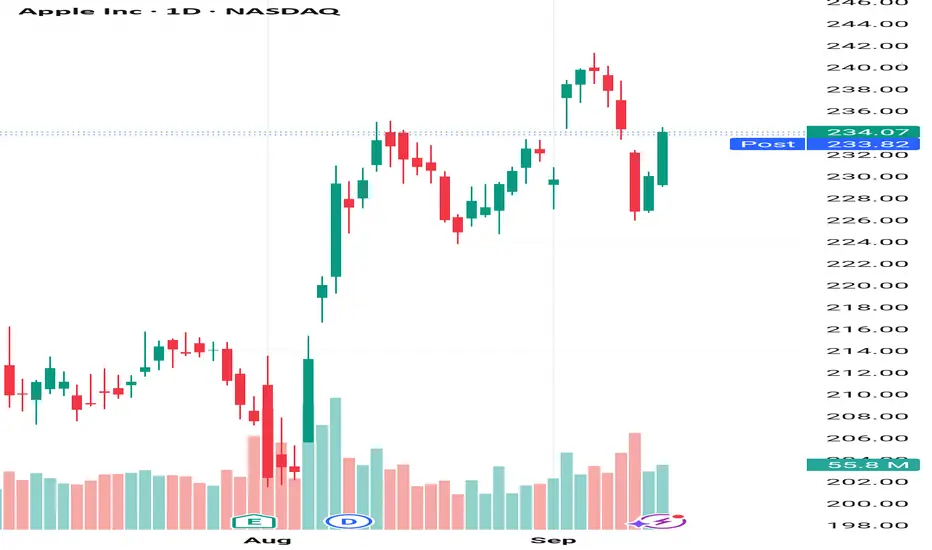
Simple UO + ADX Futures Strategy📚 Trading Plan with UO + ADX + 9/21 MA
1. Indicator Roles
Ultimate Oscillator (UO): Measures momentum across 3 different timeframes (short, medium, long). I use the lengths 4/8/14.
Overbought: > 70
Oversold: < 30
Neutral: 30–70 range
ADX (14-period, 100 smoothed): Measures trend strength, not direction.
Weak trend: < 17~20
Building trend: 20–25
Strong trend: > 27–30, enter on pullback. A bounce from the 9 or 21 MA.
2. Core Trading Logic
We combine momentum (UO) with trend strength (ADX) to avoid false signals.
Long Setup (Buy):
ADX rising above 23 → trend gaining strength.
UO crosses above 30 from below → confirms bullish momentum.
Confirm price is above 21-day MA (optional filter for trend).
📈 Exit:
UO > 50 and turning down, or
ADX below 17, or
Trailing MA.
Short Setup (Sell):
ADX rising above 27 → trend gaining strength.
UO crosses below 70 from above → confirms bearish momentum.
Confirm price is below 9-day MA (optional filter for trend).
📉 Exit:
UO < 30 and turning up, or
ADX drops below 20, or
Trailing stop.
3. Advanced Filters
Avoid false breakouts: If ADX < 20, ignore UO signals (no strong trend).
Divergence filter: If price makes a new high but UO does not → weakening trend.
Scaling:
Add to winners if ADX > 30 and still rising.
Take partial profits if ADX flattens while UO is in extreme zone.
4. Risk Management
Position sizing: Risk 1–2% of account per trade.
Stop loss: Below recent swing low (for longs) or above swing high (for shorts).
Take profit: Risk:Reward 1:2 minimum, or trail with MA.
5. Example Workflow
Case 1 (Bullish):
ADX rises from 18 → 27 (trend forming).
UO crosses 50 → bullish signal.
Enter long.
Exit when UO > 70 and rolls over, or ADX drops < 20.
Case 2 (Bearish):
ADX rises above 25.
UO crosses below 50.
Enter short.
Exit when UO < 30 and turns up, or ADX weakens.
✅ Summary Ruleset
Trade only when ADX > 23–25 (filter out noise).
Go long: UO crosses > 50 with rising ADX.
Go short: UO crosses < 50 with rising ADX.
Exit on momentum extremes (UO < 30 or > 70) or weakening ADX.
Risk: Keep losses capped at 1–2% of equity per trade.
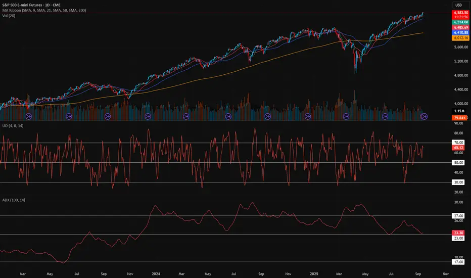
52-Week High Effect📚 52-Week High Trading Strategy
1. Core Idea
Contrary to the “buy low, sell high” mantra, this strategy buys stocks making new 52-week highs.
Rationale: Momentum effect — stocks at or near new highs tend to keep outperforming, while those far from highs underperform.
Behavioral Explanation: Investors anchor to past highs → underreact to breakouts, leaving room for continued rallies.
2. What is the 52-Week High?
The highest closing price over the past 252 trading days (≈ 1 year).
52-week range = highest close vs lowest close in that period.
A new 52-week high signals market conviction, often accompanied by higher volume.
3. Academic Evidence (The “52-Week High Effect”)
Hong, Jordan & Liu (1963–2009 study):
Buying stocks near 52-week highs & shorting those far from highs produced ~0.60% monthly returns.
Strongest effect in high-beta industries and stocks with less informative prices.
Numerous studies confirm positive drift in high-52-week stocks, while buying 52-week lows is usually a losing strategy.
4. Key Findings
Short-Term (Days–Weeks)
Buying new 52-week highs = poor results in 5–10 day windows (mean reversion dominates short term).
Shorting new highs = also unprofitable.
Takeaway: Short-term trades off new highs don’t work well.
Medium–Long-Term (Months–Years)
Buying new 52-week highs with proper exits yields positive returns, similar to 2x ETFs.
Risk-adjusted returns improve when combined with trend filters (MAs, trailing stops).
Example exit rules:
Sell if stock closes below 200-day MA.
Sell on 20% trailing stop, 21 MA.
Sell on new 20-bar low.
Momentum Portfolio Approach
Rank stocks by distance to 52-week high.
Buy top 10 with equal weights (conditions: stock above 50-day MA, S&P 500 above 200-day MA).
Rebalance weekly/monthly.
Results: Outperformed S&P 500.
Index Application
50/200 Moving Average Cross on 52-Week High: Didn’t work well (weak signals).
Breakout Rule: Buy when 52-week high index/equity makes new 9-day high, sell when it makes 9-day low → more tradable, but still mixed performance.
5. Advantages
✅ Evidence-based: Supported by decades of academic research.
✅ Simple: Easy to screen and implement.
✅ Momentum aligned: Rides strong trends.
✅ Works best in diversified portfolio format.
6. Disadvantages
❌ Not great for short-term traders (breakouts often mean-revert in 5–10 days).
❌ High drawdowns possible (44%+ in tests).
❌ Underperforms in sideways/choppy markets.
❌ Requires risk controls (stops or trend filters).
7. How to Apply in Practice
Stock Picking
TradingView Screener: Price within 15~10% of 52-week high, above 50-day & 200-day MA.
Buy breakouts when supported by volume.
Use trailing stop or moving average exit. 9 or 21 MA.
For Mega-Caps, if they are near the 52-week low, then it's a buy signal. Example, AMD, etc.
Portfolio (Momentum Rotation)
Rank S&P 500 stocks by % off 52-week high.
Buy the top 10–20 strongest names.
Rebalance monthly/quarterly.
ETFs / Index Strategy
Use 52-week high rules on sector ETFs or SPY itself.
Works best when combined with breadth indicators (e.g., % of S&P 500 stocks making new highs).
8. Key Takeaway
The 52-week high strategy is a momentum approach:
Poor short-term, but effective long-term with proper filters.
Best results come from systematic portfolios rather than single discretionary trades.
Think of it less as “chasing” and more as “joining the strongest trends early.”
✅ In one line: The 52-week high strategy exploits investor underreaction by buying stocks near new highs — it works best as a long-term momentum portfolio with trend filters, not as a short-term breakout trade.