Quant Seasonality ProQuant Seasonality Pro (QuantSeaz)
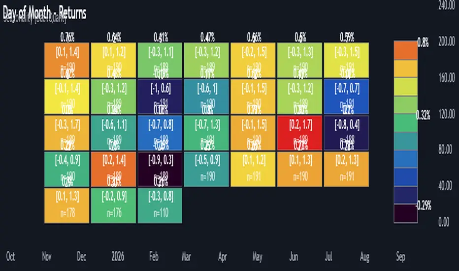
Quant Seasonality Pro is a data-driven seasonal projection tool that extracts historical day-of-year return patterns and transforms them into a forward-looking price curve. Using log returns, cycle filters, and volatility-based scaling (ATR), it generates a dynamically anchored seasonal roadmap directly on your chart.
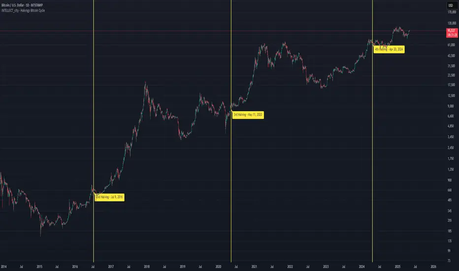
The indicator allows you to switch between Trading Days (stocks/forex) and Calendar Days (crypto), apply U.S. election cycle filters, and analyze precisly historical data. The projected curve is detrended to isolate true seasonal structure and then scaled to current market volatility for realistic visualization.
A built-in statistical dashboard provides:
Confidence (%) based on historical win rates
Expected Alpha (%) over the selected forward window
ATR % (noise level)
Viability ratio (Alpha adjusted for risk)
This tool is designed for contextual edge — not signal automation. It helps traders align positioning with historical seasonal tendencies while maintaining proper risk management and independent confirmation.
Hope you enjoy it
Pine Script® indicator