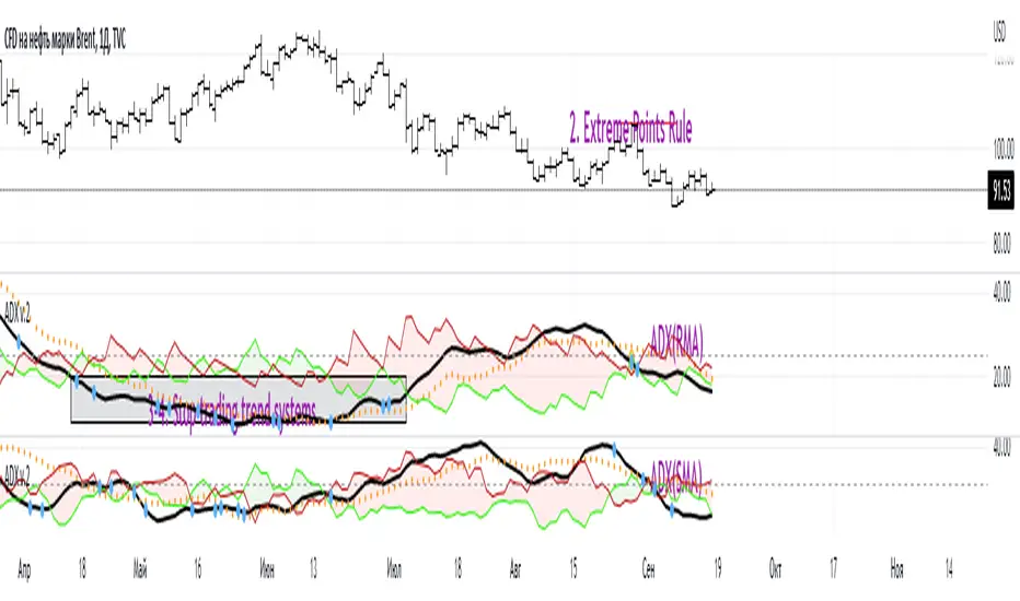
ADX W. Wilders(DI+, DI-, DX, ADXR, Equilibrium Point)The reason for publishing the script was the lack of display of important components in the standard ADX indicator, such as DI+, DI-, DX , ADXR, and the absence of a choice of methods for calculating moving averages in the indicator.
According to the book by the author of the ADX indicator, W. Wilder, the indicator components were calculated using the SMA formula, however, the RMA moving average is used in the code of the built-in indicator in TradingView, which shows excellent results, but this is not a classic calculation method. In addition to SMA and RMA, there are also EMA , HMA , WMA , VWMA moving averages to choose from. Added the ability to display lines ADX , ADXR , DX , DI+, DI- and Equilibrium points (when DI+ and DI- are equal or intersect).
ADX Trading Rules
1. Trade the intersections of DI+ and DI-
2. Extreme Point Rule(EPR). EPR is formed when DI+, DI- (Equilibrium point) crosses, forming a trend reversal point at the extremum of the current bar. In the example on the ADX RMA chart, the DI- line is above DI+. Being in a short position at the reverse intersection of the DI- and DI + lines, it is necessary to take the high price of the crossing bar for the reversal point, upon breakdown of which, turn to long. In this example, the breakdown did not take place and the short position remained active, despite the intersection of the DI+ lines over DI-. This rule is an excellent filter that removes unnecessary transactions in the trading system.
3. DI+ > ADX and DI- > ADX. Stop trading trend-following systems.
4. If ADXR > 25, the trading system will be profitable. With ADXR < 20, trend-following systems need to stop trading. Many mistakenly use ADX values instead of ADXR . The author explicitly pointed to ADXR in his book.
5. Equilibrium Point - balance points. The accumulation of these points on the chart means the presence of a flat in the market. Accumulation often appears on a declining ADX after a top has been established on the ADX indicator. The smaller the distance between the points, the less significant movements occurred in the market.
6. For intraday trading of cryptocurrencies use can the following ADX settings:
DI Length = 100
ADX Smoothing = 14
MA Type = VWMA
Flat Zone = 30
P.S. Fragment from an interview with W. Wilder:
OH: You are probably best known for inventing the Relative Strength Index ( RSI ), Average Directional Index ( ADX ) and Average True Range (ATR). Which of these is the most powerful tool for a trader?
WW: The ADX .
OH: Is it the indicator you are most proud of?
WW: I guess so.
Search in scripts for "rma"
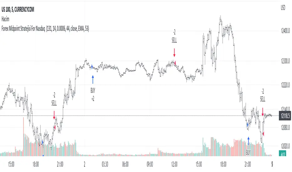
Forex Midpoint Stratejisi For Nasdaq English Knowledge:
Midpoint Strategy;
The general calculation method is a strategy that helps determine direction by the intersection of a MA line and the value obtained by dividing the lowest and highest price in the specified length range.
Başlangıç Periyodu: The data length of the Midpoint Line.
Kaydırma Seviyesi: The number of steps forward or backward of the Midpoint Line.
Yüzde Seviyesi: the amount of vertical scrolling.
Uzunluk: The length of the MA line
represents.
This strategy is prepared for the Nasdaq 5-minute period. It needs to be optimized for use on other instruments.
There are take profit and stop loss levels within the codes. Friends who want to use it can remove the invisibility from the relevant sections. Also, I removed the midpoint and the MA line so that it does not crowd the image, you can add it if you want.
Thank you.
Turkish Knowledge:
Midpoint Stratejisi;
Genel hesaplama yöntemi, belirlenen uzunluk aralığındaki en düşük ve en yüksek fiyatın ikiye bölümü ile elde edilen değer ve bir ortalama çizgisinin kesişimleriyle yön belirlemeye yardımcı bir stratejidir.
Başlangıç Period: Midpoint Çizgisinin veri uzunluğunu.
Kaydırma Seviyesi: Midpoint Çizgisinin ileri veya geri adım sayısını.
Yüzde Seviyesi: dikey kaydırma miktarını.
Uzunluk: Ortalama çizgisinin uzunluğunu
temsil etmektedir.
Bu strateji Nasdaq 5 dakikalık periot için hazırlanmıştır. Diğer enstrümanlarda kullanılması için optimize edilmesi gerekir.
Kodların içinde Kar alma , zarar durdurma seviyeleri mevcuttur. Kullanmak isteyen arkadaşlar ilgili bölümlerden görünmezliği kaldırabilirler. ayrıca midpoint ve ortalama çizgisinide görüntü kalabalığı yapmaması için ben kaldırdım isterseniz siz ekleyebilirsiniz.
Teşekkürler.
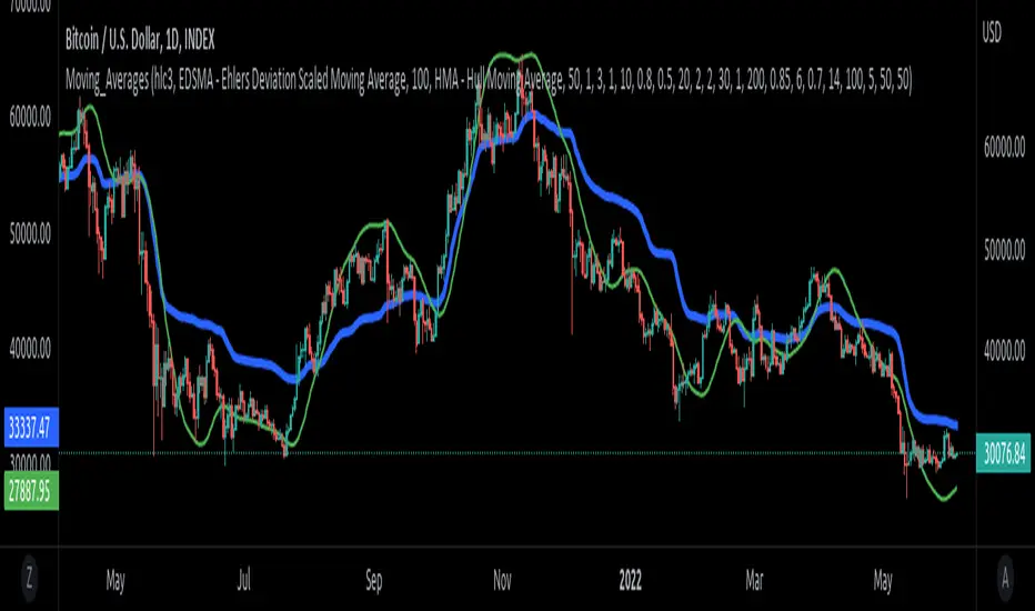
Moving_AveragesLibrary "Moving_Averages"
This library contains majority important moving average functions with int series support. Which means that they can be used with variable length input. For conventional use, please use tradingview built-in ta functions for moving averages as they are more precise. I'll use functions in this library for my other scripts with dynamic length inputs.
ema(src, len)
Exponential Moving Average (EMA)
Parameters:
src : Source
len : Period
Returns: Exponential Moving Average with Series Int Support (EMA)
alma(src, len, a_offset, a_sigma)
Arnaud Legoux Moving Average (ALMA)
Parameters:
src : Source
len : Period
a_offset : Arnaud Legoux offset
a_sigma : Arnaud Legoux sigma
Returns: Arnaud Legoux Moving Average (ALMA)
covwema(src, len)
Coefficient of Variation Weighted Exponential Moving Average (COVWEMA)
Parameters:
src : Source
len : Period
Returns: Coefficient of Variation Weighted Exponential Moving Average (COVWEMA)
covwma(src, len)
Coefficient of Variation Weighted Moving Average (COVWMA)
Parameters:
src : Source
len : Period
Returns: Coefficient of Variation Weighted Moving Average (COVWMA)
dema(src, len)
DEMA - Double Exponential Moving Average
Parameters:
src : Source
len : Period
Returns: DEMA - Double Exponential Moving Average
edsma(src, len, ssfLength, ssfPoles)
EDSMA - Ehlers Deviation Scaled Moving Average
Parameters:
src : Source
len : Period
ssfLength : EDSMA - Super Smoother Filter Length
ssfPoles : EDSMA - Super Smoother Filter Poles
Returns: Ehlers Deviation Scaled Moving Average (EDSMA)
eframa(src, len, FC, SC)
Ehlrs Modified Fractal Adaptive Moving Average (EFRAMA)
Parameters:
src : Source
len : Period
FC : Lower Shift Limit for Ehlrs Modified Fractal Adaptive Moving Average
SC : Upper Shift Limit for Ehlrs Modified Fractal Adaptive Moving Average
Returns: Ehlrs Modified Fractal Adaptive Moving Average (EFRAMA)
ehma(src, len)
EHMA - Exponential Hull Moving Average
Parameters:
src : Source
len : Period
Returns: Exponential Hull Moving Average (EHMA)
etma(src, len)
Exponential Triangular Moving Average (ETMA)
Parameters:
src : Source
len : Period
Returns: Exponential Triangular Moving Average (ETMA)
frama(src, len)
Fractal Adaptive Moving Average (FRAMA)
Parameters:
src : Source
len : Period
Returns: Fractal Adaptive Moving Average (FRAMA)
hma(src, len)
HMA - Hull Moving Average
Parameters:
src : Source
len : Period
Returns: Hull Moving Average (HMA)
jma(src, len, jurik_phase, jurik_power)
Jurik Moving Average - JMA
Parameters:
src : Source
len : Period
jurik_phase : Jurik (JMA) Only - Phase
jurik_power : Jurik (JMA) Only - Power
Returns: Jurik Moving Average (JMA)
kama(src, len, k_fastLength, k_slowLength)
Kaufman's Adaptive Moving Average (KAMA)
Parameters:
src : Source
len : Period
k_fastLength : Number of periods for the fastest exponential moving average
k_slowLength : Number of periods for the slowest exponential moving average
Returns: Kaufman's Adaptive Moving Average (KAMA)
kijun(_high, _low, len, kidiv)
Kijun v2
Parameters:
_high : High value of bar
_low : Low value of bar
len : Period
kidiv : Kijun MOD Divider
Returns: Kijun v2
lsma(src, len, offset)
LSMA/LRC - Least Squares Moving Average / Linear Regression Curve
Parameters:
src : Source
len : Period
offset : Offset
Returns: Least Squares Moving Average (LSMA)/ Linear Regression Curve (LRC)
mf(src, len, beta, feedback, z)
MF - Modular Filter
Parameters:
src : Source
len : Period
beta : Modular Filter, General Filter Only - Beta
feedback : Modular Filter Only - Feedback
z : Modular Filter Only - Feedback Weighting
Returns: Modular Filter (MF)
rma(src, len)
RMA - RSI Moving average
Parameters:
src : Source
len : Period
Returns: RSI Moving average (RMA)
sma(src, len)
SMA - Simple Moving Average
Parameters:
src : Source
len : Period
Returns: Simple Moving Average (SMA)
smma(src, len)
Smoothed Moving Average (SMMA)
Parameters:
src : Source
len : Period
Returns: Smoothed Moving Average (SMMA)
stma(src, len)
Simple Triangular Moving Average (STMA)
Parameters:
src : Source
len : Period
Returns: Simple Triangular Moving Average (STMA)
tema(src, len)
TEMA - Triple Exponential Moving Average
Parameters:
src : Source
len : Period
Returns: Triple Exponential Moving Average (TEMA)
thma(src, len)
THMA - Triple Hull Moving Average
Parameters:
src : Source
len : Period
Returns: Triple Hull Moving Average (THMA)
vama(src, len, volatility_lookback)
VAMA - Volatility Adjusted Moving Average
Parameters:
src : Source
len : Period
volatility_lookback : Volatility lookback length
Returns: Volatility Adjusted Moving Average (VAMA)
vidya(src, len)
Variable Index Dynamic Average (VIDYA)
Parameters:
src : Source
len : Period
Returns: Variable Index Dynamic Average (VIDYA)
vwma(src, len)
Volume-Weighted Moving Average (VWMA)
Parameters:
src : Source
len : Period
Returns: Volume-Weighted Moving Average (VWMA)
wma(src, len)
WMA - Weighted Moving Average
Parameters:
src : Source
len : Period
Returns: Weighted Moving Average (WMA)
zema(src, len)
Zero-Lag Exponential Moving Average (ZEMA)
Parameters:
src : Source
len : Period
Returns: Zero-Lag Exponential Moving Average (ZEMA)
zsma(src, len)
Zero-Lag Simple Moving Average (ZSMA)
Parameters:
src : Source
len : Period
Returns: Zero-Lag Simple Moving Average (ZSMA)
evwma(src, len)
EVWMA - Elastic Volume Weighted Moving Average
Parameters:
src : Source
len : Period
Returns: Elastic Volume Weighted Moving Average (EVWMA)
tt3(src, len, a1_t3)
Tillson T3
Parameters:
src : Source
len : Period
a1_t3 : Tillson T3 Volume Factor
Returns: Tillson T3
gma(src, len)
GMA - Geometric Moving Average
Parameters:
src : Source
len : Period
Returns: Geometric Moving Average (GMA)
wwma(src, len)
WWMA - Welles Wilder Moving Average
Parameters:
src : Source
len : Period
Returns: Welles Wilder Moving Average (WWMA)
ama(src, _high, _low, len, ama_f_length, ama_s_length)
AMA - Adjusted Moving Average
Parameters:
src : Source
_high : High value of bar
_low : Low value of bar
len : Period
ama_f_length : Fast EMA Length
ama_s_length : Slow EMA Length
Returns: Adjusted Moving Average (AMA)
cma(src, len)
Corrective Moving average (CMA)
Parameters:
src : Source
len : Period
Returns: Corrective Moving average (CMA)
gmma(src, len)
Geometric Mean Moving Average (GMMA)
Parameters:
src : Source
len : Period
Returns: Geometric Mean Moving Average (GMMA)
ealf(src, len, LAPercLen_, FPerc_)
Ehler's Adaptive Laguerre filter (EALF)
Parameters:
src : Source
len : Period
LAPercLen_ : Median Length
FPerc_ : Median Percentage
Returns: Ehler's Adaptive Laguerre filter (EALF)
elf(src, len, LAPercLen_, FPerc_)
ELF - Ehler's Laguerre filter
Parameters:
src : Source
len : Period
LAPercLen_ : Median Length
FPerc_ : Median Percentage
Returns: Ehler's Laguerre Filter (ELF)
edma(src, len)
Exponentially Deviating Moving Average (MZ EDMA)
Parameters:
src : Source
len : Period
Returns: Exponentially Deviating Moving Average (MZ EDMA)
pnr(src, len, rank_inter_Perc_)
PNR - percentile nearest rank
Parameters:
src : Source
len : Period
rank_inter_Perc_ : Rank and Interpolation Percentage
Returns: Percentile Nearest Rank (PNR)
pli(src, len, rank_inter_Perc_)
PLI - Percentile Linear Interpolation
Parameters:
src : Source
len : Period
rank_inter_Perc_ : Rank and Interpolation Percentage
Returns: Percentile Linear Interpolation (PLI)
rema(src, len)
Range EMA (REMA)
Parameters:
src : Source
len : Period
Returns: Range EMA (REMA)
sw_ma(src, len)
Sine-Weighted Moving Average (SW-MA)
Parameters:
src : Source
len : Period
Returns: Sine-Weighted Moving Average (SW-MA)
vwap(src, len)
Volume Weighted Average Price (VWAP)
Parameters:
src : Source
len : Period
Returns: Volume Weighted Average Price (VWAP)
mama(src, len)
MAMA - MESA Adaptive Moving Average
Parameters:
src : Source
len : Period
Returns: MESA Adaptive Moving Average (MAMA)
fama(src, len)
FAMA - Following Adaptive Moving Average
Parameters:
src : Source
len : Period
Returns: Following Adaptive Moving Average (FAMA)
hkama(src, len)
HKAMA - Hilbert based Kaufman's Adaptive Moving Average
Parameters:
src : Source
len : Period
Returns: Hilbert based Kaufman's Adaptive Moving Average (HKAMA)
AMASling - All Moving Average Sling ShotThis indicator modifies the SlingShot System by Chris Moody to allow it to be based on 'any' Fast and Slow moving average pair. Open Long / Close Long / Open Short / Close Short alerts can be generated for automated bot trading based on the SlingShot strategy:
• Conservative Entry = Fast MA above Slow MA, and previous bar close below Fast MA, and current price above Fast MA
• Conservative Entry = Fast MA below Slow MA, and previous bar close above Fast MA, and current price below Fast MA
• Aggressive Entry = Fast MA above Slow MA, and price below Fast MA
• Aggressive Exit = Fast MA below Slow MA, and price above Fast MA
Entries and exits can also be made based on moving average crossovers, I initially put this in to make it easy to compare to a more standard strategy, but upon backtesting combining crossovers with the SlingShot appeared to produce better results on some charts.
Alerts can also be filtered to allow long deals only when the fast moving average is above the slow moving average (uptrend) and short deals only when the fast moving average is below the slow moving averages (downtrend).
If you have a strategy that can buy based on External Indicators you can use the 'Backtest Signal' which plots the values set in the 'Long / Short Signals' section.
The Fast, Slow and Signal Moving Averages can be set to:
• Simple Moving Average (SMA)
• Exponential Moving Average (EMA)
• Weighted Moving Average (WMA)
• Volume-Weighted Moving Average (VWMA)
• Hull Moving Average (HMA)
• Exponentially Weighted Moving Average (RMA) (SMMA)
• Linear regression curve Moving Average (LSMA)
• Double EMA (DEMA)
• Double SMA (DSMA)
• Double WMA (DWMA)
• Double RMA (DRMA)
• Triple EMA (TEMA)
• Triple SMA (TSMA)
• Triple WMA (TWMA)
• Triple RMA (TRMA)
• Symmetrically Weighted Moving Average (SWMA) ** length does not apply **
• Arnaud Legoux Moving Average (ALMA)
• Variable Index Dynamic Average (VIDYA)
• Fractal Adaptive Moving Average (FRAMA)
'Backtest Signal' and 'Deal State' are plotted to display.none, so change the Style Settings for the chart if you need to see them for testing.
Yes I did choose the name because 'It's Amasling!'

pandas_taLibrary "pandas_ta"
Level: 3
Background
Today is the first day of 2022 and happy new year every tradingviewers! May health and wealth go along with you all the time. I use this chance to publish my 1st PINE v5 lib : pandas_ta
This is not a piece of cake like thing, which cost me a lot of time and efforts to build this lib. Beyond 300 versions of this script was iterated in draft.
Function
Library "pandas_ta"
PINE v5 Counterpart of Pandas TA - A Technical Analysis Library in Python 3 at github.com
The Original Pandas Technical Analysis (Pandas TA) is an easy to use library that leverages the Pandas package with more than 130 Indicators and Utility functions and more than 60 TA Lib Candlestick Patterns.
I realized most of indicators except Candlestick Patterns because tradingview built-in Candlestick Patterns are even more powerful!
I use this to verify pandas_ta python version indicators for myself, but I realize that maybe many may need similar lib for pine v5 as well.
Function Brief Descriptions (Pls find details in script comments)
bton --> Binary to number
wcp --> Weighted Closing Price (WCP)
counter --> Condition counter
xbt --> Between
ebsw --> Even Better SineWave (EBSW)
ao --> Awesome Oscillator (AO)
apo --> Absolute Price Oscillator (APO)
xrf --> Dynamic shifted values
bias --> Bias (BIAS)
bop --> Balance of Power (BOP)
brar --> BRAR (BRAR)
cci --> Commodity Channel Index (CCI)
cfo --> Chande Forcast Oscillator (CFO)
cg --> Center of Gravity (CG)
cmo --> Chande Momentum Oscillator (CMO)
coppock --> Coppock Curve (COPC)
cti --> Correlation Trend Indicator (CTI)
dmi --> Directional Movement Index(DMI)
er --> Efficiency Ratio (ER)
eri --> Elder Ray Index (ERI)
fisher --> Fisher Transform (FISHT)
inertia --> Inertia (INERTIA)
kdj --> KDJ (KDJ)
kst --> 'Know Sure Thing' (KST)
macd --> Moving Average Convergence Divergence (MACD)
mom --> Momentum (MOM)
pgo --> Pretty Good Oscillator (PGO)
ppo --> Percentage Price Oscillator (PPO)
psl --> Psychological Line (PSL)
pvo --> Percentage Volume Oscillator (PVO)
qqe --> Quantitative Qualitative Estimation (QQE)
roc --> Rate of Change (ROC)
rsi --> Relative Strength Index (RSI)
rsx --> Relative Strength Xtra (rsx)
rvgi --> Relative Vigor Index (RVGI)
slope --> Slope
smi --> SMI Ergodic Indicator (SMI)
sqz* --> Squeeze (SQZ) * NOTE: code sufferred from very strange error, code was commented.
sqz_pro --> Squeeze PRO(SQZPRO)
xfl --> Condition filter
stc --> Schaff Trend Cycle (STC)
stoch --> Stochastic (STOCH)
stochrsi --> Stochastic RSI (STOCH RSI)
trix --> Trix (TRIX)
tsi --> True Strength Index (TSI)
uo --> Ultimate Oscillator (UO)
willr --> William's Percent R (WILLR)
alma --> Arnaud Legoux Moving Average (ALMA)
xll --> Dynamic rolling lowest values
dema --> Double Exponential Moving Average (DEMA)
ema --> Exponential Moving Average (EMA)
fwma --> Fibonacci's Weighted Moving Average (FWMA)
hilo --> Gann HiLo Activator(HiLo)
hma --> Hull Moving Average (HMA)
hwma --> HWMA (Holt-Winter Moving Average)
ichimoku --> Ichimoku Kinkō Hyō (ichimoku)
jma --> Jurik Moving Average Average (JMA)
kama --> Kaufman's Adaptive Moving Average (KAMA)
linreg --> Linear Regression Moving Average (linreg)
mgcd --> McGinley Dynamic Indicator
rma --> wildeR's Moving Average (RMA)
sinwma --> Sine Weighted Moving Average (SWMA)
ssf --> Ehler's Super Smoother Filter (SSF) © 2013
supertrend --> Supertrend (supertrend)
xsa --> X simple moving average
swma --> Symmetric Weighted Moving Average (SWMA)
t3 --> Tim Tillson's T3 Moving Average (T3)
tema --> Triple Exponential Moving Average (TEMA)
trima --> Triangular Moving Average (TRIMA)
vidya --> Variable Index Dynamic Average (VIDYA)
vwap --> Volume Weighted Average Price (VWAP)
vwma --> Volume Weighted Moving Average (VWMA)
wma --> Weighted Moving Average (WMA)
zlma --> Zero Lag Moving Average (ZLMA)
entropy --> Entropy (ENTP)
kurtosis --> Rolling Kurtosis
skew --> Rolling Skew
xev --> Condition all
zscore --> Rolling Z Score
adx --> Average Directional Movement (ADX)
aroon --> Aroon & Aroon Oscillator (AROON)
chop --> Choppiness Index (CHOP)
xex --> Condition any
cksp --> Chande Kroll Stop (CKSP)
dpo --> Detrend Price Oscillator (DPO)
long_run --> Long Run
psar --> Parabolic Stop and Reverse (psar)
short_run --> Short Run
vhf --> Vertical Horizontal Filter (VHF)
vortex --> Vortex
accbands --> Acceleration Bands (ACCBANDS)
atr --> Average True Range (ATR)
bbands --> Bollinger Bands (BBANDS)
donchian --> Donchian Channels (DC)
kc --> Keltner Channels (KC)
massi --> Mass Index (MASSI)
natr --> Normalized Average True Range (NATR)
pdist --> Price Distance (PDIST)
rvi --> Relative Volatility Index (RVI)
thermo --> Elders Thermometer (THERMO)
ui --> Ulcer Index (UI)
ad --> Accumulation/Distribution (AD)
cmf --> Chaikin Money Flow (CMF)
efi --> Elder's Force Index (EFI)
ecm --> Ease of Movement (EOM)
kvo --> Klinger Volume Oscillator (KVO)
mfi --> Money Flow Index (MFI)
nvi --> Negative Volume Index (NVI)
obv --> On Balance Volume (OBV)
pvi --> Positive Volume Index (PVI)
dvdi --> Dual Volume Divergence Index (DVDI)
xhh --> Dynamic rolling highest values
pvt --> Price-Volume Trend (PVT)
Remarks
I also incorporated func descriptions and func test script in commented mode, you can test the functino with the embedded test script and modify them as you wish.
This is a Level 3 free and open source indicator library.
Feedbacks are appreciated.
This is not the end of pandas_ta lib publication, but it is start point with pine v5 lib function and I will add more and more funcs into this lib for my own indicators.
Function Name List:
bton()
wcp()
count()
xbt()
ebsw()
ao()
apo()
xrf()
bias()
bop()
brar()
cci()
cfo()
cg()
cmo()
coppock()
cti()
dmi()
er()
eri()
fisher()
inertia()
kdj()
kst()
macd()
mom()
pgo()
ppo()
psl()
pvo()
qqe()
roc()
rsi()
rsx()
rvgi()
slope()
smi()
sqz_pro()
xfl()
stc()
stoch()
stochrsi()
trix()
tsi()
uo()
willr()
alma()
wcx()
xll()
dema()
ema()
fwma()
hilo()
hma()
hwma()
ichimoku()
jma()
kama()
linreg()
mgcd()
rma()
sinwma()
ssf()
supertrend()
xsa()
swma()
t3()
tema()
trima()
vidya()
vwap()
vwma()
wma()
zlma()
entropy()
kurtosis()
skew()
xev()
zscore()
adx()
aroon()
chop()
xex()
cksp()
dpo()
long_run()
psar()
short_run()
vhf()
vortex()
accbands()
atr()
bbands()
donchian()
kc()
massi()
natr()
pdist()
rvi()
thermo()
ui()
ad()
cmf()
efi()
ecm()
kvo()
mfi()
nvi()
obv()
pvi()
dvdi()
xhh()
pvt()

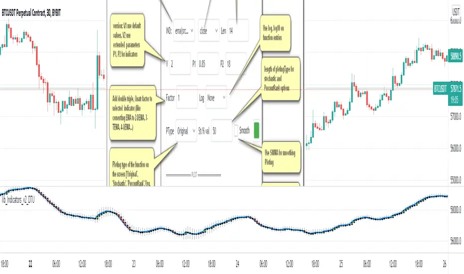
Indicator Functions with Factor and HeikinAshiHello all,
This indicator returns below selected indicators values with entered parameters.
Also you can add factorization, functions candles, function HeikinAshi and more to the plot.
VERSION:
Version 1: returns series only source and Length with already defined default values
Version 2: returns series with source, Length, p1 and p2 parameters according to the indicator definition (ex: )
PARAMETERS p1 p2
for defining multi arguments (See indicators list) indicator input value usable with verison=V2 selected.. ex: for alma( src , len ,offset=0.85,sigma=6), set source=source, len=length, p1=0.85 an p2=6
FACTOR:
Add double triple, Quadruple factors to selected indicator (like converting EMA to 2-DEMA, 3-TEMA, 4-QEMA...)
1-Original
2-Double
3-Triple
4-Quadruple
LOG
Log: Use log, log10 on function entries
PLOTTING:
PType: Plotting type of the function on the screen
Original :use original values
Org. Range (-1,1): usable for indicators between range -1 and 1
Stochastic: Convert indicator values by using stochastic calculation between -1 & 1. (use AT/% length to better view)
PercentRank: Convert indicator values by using Percent Rank calculation between -1 & 1. (use AT/% length to better view)
ST/%: length for plotting Type for stochastic and Percent Rank options
Smooth: Use SWMA for smoothing the function
DISPLAY TYPES
Plot Candles: Display the selected indicator as candle by implementing values
Plot Ind: Display result of indicator with selected source
HeikinAshi: Display Selected indicator candles with Heikin Ashi calculation
INDICATOR LIST:
hide = 'DONT DISPLAY', //Dont display & calculate the indicator. (For my framework usage)
alma = 'alma( src , len ,offset=0.85,sigma=6)', // Arnaud Legoux Moving Average
ama = 'ama( src , len ,fast=14,slow=100)', //Adjusted Moving Average
acdst = 'accdist()', // Accumulation/distribution index.
cma = 'cma( src , len )', //Corrective Moving average
dema = 'dema( src , len )', // Double EMA (Same as EMA with 2 factor)
ema = 'ema( src , len )', // Exponential Moving Average
gmma = 'gmma( src , len )', //Geometric Mean Moving Average
hghst = 'highest( src , len )', //Highest value for a given number of bars back.
hl2ma = 'hl2ma( src , len )', //higest lowest moving average
hma = 'hma( src , len )', // Hull Moving Average .
lgAdt = 'lagAdapt( src , len ,perclen=5,fperc=50)', //Ehler's Adaptive Laguerre filter
lgAdV = 'lagAdaptV( src , len ,perclen=5,fperc=50)', //Ehler's Adaptive Laguerre filter variation
lguer = 'laguerre( src , len )', //Ehler's Laguerre filter
lsrcp = 'lesrcp( src , len )', //lowest exponential esrcpanding moving line
lexp = 'lexp( src , len )', //lowest exponential expanding moving line
linrg = 'linreg( src , len ,loffset=1)', // Linear regression
lowst = 'lowest( src , len )', //Lovest value for a given number of bars back.
pcnl = 'percntl( src , len )', //percentile nearest rank. Calculates percentile using method of Nearest Rank.
pcnli = 'percntli( src , len )', //percentile linear interpolation. Calculates percentile using method of linear interpolation between the two nearest ranks.
rema = 'rema( src , len )', //Range EMA (REMA)
rma = 'rma( src , len )', //Moving average used in RSI . It is the exponentially weighted moving average with alpha = 1 / length.
sma = 'sma( src , len )', // Smoothed Moving Average
smma = 'smma( src , len )', // Smoothed Moving Average
supr2 = 'super2( src , len )', //Ehler's super smoother, 2 pole
supr3 = 'super3( src , len )', //Ehler's super smoother, 3 pole
strnd = 'supertrend( src , len ,period=3)', //Supertrend indicator
swma = 'swma( src , len )', //Sine-Weighted Moving Average
tema = 'tema( src , len )', // Triple EMA (Same as EMA with 3 factor)
tma = 'tma( src , len )', //Triangular Moving Average
vida = 'vida( src , len )', // Variable Index Dynamic Average
vwma = 'vwma( src , len )', // Volume Weigted Moving Average
wma = 'wma( src , len )', //Weigted Moving Average
angle = 'angle( src , len )', //angle of the series (Use its Input as another indicator output)
atr = 'atr( src , len )', // average true range . RMA of true range.
bbr = 'bbr( src , len ,mult=1)', // bollinger %%
bbw = 'bbw( src , len ,mult=2)', // Bollinger Bands Width . The Bollinger Band Width is the difference between the upper and the lower Bollinger Bands divided by the middle band.
cci = 'cci( src , len )', // commodity channel index
cctbb = 'cctbbo( src , len )', // CCT Bollinger Band Oscilator
chng = 'change( src , len )', //Difference between current value and previous, source - source.
cmo = 'cmo( src , len )', // Chande Momentum Oscillator . Calculates the difference between the sum of recent gains and the sum of recent losses and then divides the result by the sum of all price movement over the same period.
cog = 'cog( src , len )', //The cog (center of gravity ) is an indicator based on statistics and the Fibonacci golden ratio.
cpcrv = 'copcurve( src , len )', // Coppock Curve. was originally developed by Edwin "Sedge" Coppock (Barron's Magazine, October 1962).
corrl = 'correl( src , len )', // Correlation coefficient . Describes the degree to which two series tend to deviate from their ta. sma values.
count = 'count( src , len )', //green avg - red avg
dev = 'dev( src , len )', //ta.dev() Measure of difference between the series and it's ta. sma
fall = 'falling( src , len )', //ta.falling() Test if the `source` series is now falling for `length` bars long. (Use its Input as another indicator output)
kcr = 'kcr( src , len ,mult=2)', // Keltner Channels Range
kcw = 'kcw( src , len ,mult=2)', //ta.kcw(). Keltner Channels Width. The Keltner Channels Width is the difference between the upper and the lower Keltner Channels divided by the middle channel.
macd = 'macd( src , len )', // macd
mfi = 'mfi( src , len )', // Money Flow Index
nvi = 'nvi()', // Negative Volume Index
obv = 'obv()', // On Balance Volume
pvi = 'pvi()', // Positive Volume Index
pvt = 'pvt()', // Price Volume Trend
rise = 'rising( src , len )', //ta.rising() Test if the `source` series is now rising for `length` bars long. (Use its Input as another indicator output)
roc = 'roc( src , len )', // Rate of Change
rsi = 'rsi( src , len )', // Relative strength Index
smosc = 'smi_osc( src , len ,fast=5, slow=34)', //smi Oscillator
smsig = 'smi_sig( src , len ,fast=5, slow=34)', //smi Signal
stdev = 'stdev( src , len )', //Standart deviation
trix = 'trix( src , len )' , //the rate of change of a triple exponentially smoothed moving average .
tsi = 'tsi( src , len )', //True Strength Index
vari = 'variance( src , len )', //ta.variance(). Variance is the expectation of the squared deviation of a series from its mean (ta. sma ), and it informally measures how far a set of numbers are spread out from their mean.
wilpc = 'willprc( src , len )', // Williams %R
wad = 'wad()', // Williams Accumulation/Distribution .
wvad = 'wvad()' //Williams Variable Accumulation/Distribution
I will update the indicator list when I will update the library
Thanks to tradingview, @RodrigoKazuma for their open source indicators

lib_Indicators_v2_DTULibrary "lib_Indicators_v2_DTU"
This library functions returns included Moving averages, indicators with factorization, functions candles, function heikinashi and more.
Created it to feed as backend of my indicator/strategy "Indicators & Combinations Framework Advanced v2 " that will be released ASAP.
This is replacement of my previous indicator (lib_indicators_DT)
I will add an indicator example which will use this indicator named as "lib_indicators_v2_DTU example" to help the usage of this library
Additionally library will be updated with more indicators in the future
NOTES:
Indicator functions returns only one series :-(
plotcandle function returns candle series
INDICATOR LIST:
hide = 'DONT DISPLAY', //Dont display & calculate the indicator. (For my framework usage)
alma = 'alma(src,len,offset=0.85,sigma=6)', //Arnaud Legoux Moving Average
ama = 'ama(src,len,fast=14,slow=100)', //Adjusted Moving Average
acdst = 'accdist()', //Accumulation/distribution index.
cma = 'cma(src,len)', //Corrective Moving average
dema = 'dema(src,len)', //Double EMA (Same as EMA with 2 factor)
ema = 'ema(src,len)', //Exponential Moving Average
gmma = 'gmma(src,len)', //Geometric Mean Moving Average
hghst = 'highest(src,len)', //Highest value for a given number of bars back.
hl2ma = 'hl2ma(src,len)', //higest lowest moving average
hma = 'hma(src,len)', //Hull Moving Average.
lgAdt = 'lagAdapt(src,len,perclen=5,fperc=50)', //Ehler's Adaptive Laguerre filter
lgAdV = 'lagAdaptV(src,len,perclen=5,fperc=50)', //Ehler's Adaptive Laguerre filter variation
lguer = 'laguerre(src,len)', //Ehler's Laguerre filter
lsrcp = 'lesrcp(src,len)', //lowest exponential esrcpanding moving line
lexp = 'lexp(src,len)', //lowest exponential expanding moving line
linrg = 'linreg(src,len,loffset=1)', //Linear regression
lowst = 'lowest(src,len)', //Lovest value for a given number of bars back.
pcnl = 'percntl(src,len)', //percentile nearest rank. Calculates percentile using method of Nearest Rank.
pcnli = 'percntli(src,len)', //percentile linear interpolation. Calculates percentile using method of linear interpolation between the two nearest ranks.
rema = 'rema(src,len)', //Range EMA (REMA)
rma = 'rma(src,len)', //Moving average used in RSI. It is the exponentially weighted moving average with alpha = 1 / length.
sma = 'sma(src,len)', //Smoothed Moving Average
smma = 'smma(src,len)', //Smoothed Moving Average
supr2 = 'super2(src,len)', //Ehler's super smoother, 2 pole
supr3 = 'super3(src,len)', //Ehler's super smoother, 3 pole
strnd = 'supertrend(src,len,period=3)', //Supertrend indicator
swma = 'swma(src,len)', //Sine-Weighted Moving Average
tema = 'tema(src,len)', //Triple EMA (Same as EMA with 3 factor)
tma = 'tma(src,len)', //Triangular Moving Average
vida = 'vida(src,len)', //Variable Index Dynamic Average
vwma = 'vwma(src,len)', //Volume Weigted Moving Average
wma = 'wma(src,len)', //Weigted Moving Average
angle = 'angle(src,len)', //angle of the series (Use its Input as another indicator output)
atr = 'atr(src,len)', //average true range. RMA of true range.
bbr = 'bbr(src,len,mult=1)', //bollinger %%
bbw = 'bbw(src,len,mult=2)', //Bollinger Bands Width. The Bollinger Band Width is the difference between the upper and the lower Bollinger Bands divided by the middle band.
cci = 'cci(src,len)', //commodity channel index
cctbb = 'cctbbo(src,len)', //CCT Bollinger Band Oscilator
chng = 'change(src,len)', //Difference between current value and previous, source - source .
cmo = 'cmo(src,len)', //Chande Momentum Oscillator. Calculates the difference between the sum of recent gains and the sum of recent losses and then divides the result by the sum of all price movement over the same period.
cog = 'cog(src,len)', //The cog (center of gravity) is an indicator based on statistics and the Fibonacci golden ratio.
cpcrv = 'copcurve(src,len)', //Coppock Curve. was originally developed by Edwin "Sedge" Coppock (Barron's Magazine, October 1962).
corrl = 'correl(src,len)', //Correlation coefficient. Describes the degree to which two series tend to deviate from their ta.sma values.
count = 'count(src,len)', //green avg - red avg
dev = 'dev(src,len)', //ta.dev() Measure of difference between the series and it's ta.sma
fall = 'falling(src,len)', //ta.falling() Test if the `source` series is now falling for `length` bars long. (Use its Input as another indicator output)
kcr = 'kcr(src,len,mult=2)', //Keltner Channels Range
kcw = 'kcw(src,len,mult=2)', //ta.kcw(). Keltner Channels Width. The Keltner Channels Width is the difference between the upper and the lower Keltner Channels divided by the middle channel.
macd = 'macd(src,len)', //macd
mfi = 'mfi(src,len)', //Money Flow Index
nvi = 'nvi()', //Negative Volume Index
obv = 'obv()', //On Balance Volume
pvi = 'pvi()', //Positive Volume Index
pvt = 'pvt()', //Price Volume Trend
rise = 'rising(src,len)', //ta.rising() Test if the `source` series is now rising for `length` bars long. (Use its Input as another indicator output)
roc = 'roc(src,len)', //Rate of Change
rsi = 'rsi(src,len)', //Relative strength Index
smosc = 'smi_osc(src,len,fast=5, slow=34)', //smi Oscillator
smsig = 'smi_sig(src,len,fast=5, slow=34)', //smi Signal
stdev = 'stdev(src,len)', //Standart deviation
trix = 'trix(src,len)' , //the rate of change of a triple exponentially smoothed moving average.
tsi = 'tsi(src,len)', //True Strength Index
vari = 'variance(src,len)', //ta.variance(). Variance is the expectation of the squared deviation of a series from its mean (ta.sma), and it informally measures how far a set of numbers are spread out from their mean.
wilpc = 'willprc(src,len)', //Williams %R
wad = 'wad()', //Williams Accumulation/Distribution.
wvad = 'wvad()' //Williams Variable Accumulation/Distribution.
}
f_func(string, float, simple, float, float, float, simple) f_func Return selected indicator value with different parameters. New version. Use extra parameters for available indicators
Parameters:
string : FuncType_ indicator from the indicator list
float : src_ close, open, high, low,hl2, hlc3, ohlc4 or any
simple : int length_ indicator length
float : p1 extra parameter-1. active on Version 2 for defining multi arguments indicator input value. ex: lagAdapt(src_, length_,LAPercLen_=p1,FPerc_=p2)
float : p2 extra parameter-2. active on Version 2 for defining multi arguments indicator input value. ex: lagAdapt(src_, length_,LAPercLen_=p1,FPerc_=p2)
float : p3 extra parameter-3. active on Version 2 for defining multi arguments indicator input value. ex: lagAdapt(src_, length_,LAPercLen_=p1,FPerc_=p2)
simple : int version_ indicator version for backward compatibility. V1:dont use extra parameters p1,p2,p3 and use default values. V2: use extra parameters for available indicators
Returns: float Return calculated indicator value
fn_heikin(float, float, float, float) fn_heikin Return given src data (open, high,low,close) as heikin ashi candle values
Parameters:
float : o_ open value
float : h_ high value
float : l_ low value
float : c_ close value
Returns: float heikin ashi open, high,low,close vlues that will be used with plotcandle
fn_plotFunction(float, string, simple, bool) fn_plotFunction Return input src data with different plotting options
Parameters:
float : src_ indicator src_data or any other series.....
string : plotingType Ploting type of the function on the screen
simple : int stochlen_ length for plotingType for stochastic and PercentRank options
bool : plotSWMA Use SWMA for smoothing Ploting
Returns: float
fn_funcPlotV2(string, float, simple, float, float, float, simple, string, simple, bool, bool) fn_funcPlotV2 Return selected indicator value with different parameters. New version. Use extra parameters fora available indicators
Parameters:
string : FuncType_ indicator from the indicator list
float : src_data_ close, open, high, low,hl2, hlc3, ohlc4 or any
simple : int length_ indicator length
float : p1 extra parameter-1. active on Version 2 for defining multi arguments indicator input value. ex: lagAdapt(src_, length_,LAPercLen_=p1,FPerc_=p2)
float : p2 extra parameter-2. active on Version 2 for defining multi arguments indicator input value. ex: lagAdapt(src_, length_,LAPercLen_=p1,FPerc_=p2)
float : p3 extra parameter-3. active on Version 2 for defining multi arguments indicator input value. ex: lagAdapt(src_, length_,LAPercLen_=p1,FPerc_=p2)
simple : int version_ indicator version for backward compatibility. V1:dont use extra parameters p1,p2,p3 and use default values. V2: use extra parameters for available indicators
string : plotingType Ploting type of the function on the screen
simple : int stochlen_ length for plotingType for stochastic and PercentRank options
bool : plotSWMA Use SWMA for smoothing Ploting
bool : log_ Use log on function entries
Returns: float Return calculated indicator value
fn_factor(string, float, simple, float, float, float, simple, simple, string, simple, bool, bool) fn_factor Return selected indicator's factorization with given arguments
Parameters:
string : FuncType_ indicator from the indicator list
float : src_data_ close, open, high, low,hl2, hlc3, ohlc4 or any
simple : int length_ indicator length
float : p1 parameter-1. active on Version 2 for defining multi arguments indicator input value. ex: lagAdapt(src_, length_,LAPercLen_=p1,FPerc_=p2)
float : p2 parameter-2. active on Version 2 for defining multi arguments indicator input value. ex: lagAdapt(src_, length_,LAPercLen_=p1,FPerc_=p2)
float : p3 parameter-3. active on Version 2 for defining multi arguments indicator input value. ex: lagAdapt(src_, length_,LAPercLen_=p1,FPerc_=p2)
simple : int version_ indicator version for backward compatibility. V1:dont use extra parameters p1,p2,p3 and use default values. V2: use extra parameters for available indicators
simple : int fact_ Add double triple, Quatr factor to selected indicator (like converting EMA to 2-DEMA, 3-TEMA, 4-QEMA...)
string : plotingType Ploting type of the function on the screen
simple : int stochlen_ length for plotingType for stochastic and PercentRank options
bool : plotSWMA Use SWMA for smoothing Ploting
bool : log_ Use log on function entries
Returns: float Return result of the function
fn_plotCandles(string, simple, float, float, float, simple, string, simple, bool, bool, bool) fn_plotCandles Return selected indicator's candle values with different parameters also heikinashi is available
Parameters:
string : FuncType_ indicator from the indicator list
simple : int length_ indicator length
float : p1 parameter-1. active on Version 2 for defining multi arguments indicator input value. ex: lagAdapt(src_, length_,LAPercLen_=p1,FPerc_=p2)
float : p2 parameter-2. active on Version 2 for defining multi arguments indicator input value. ex: lagAdapt(src_, length_,LAPercLen_=p1,FPerc_=p2)
float : p3 parameter-3. active on Version 2 for defining multi arguments indicator input value. ex: lagAdapt(src_, length_,LAPercLen_=p1,FPerc_=p2)
simple : int version_ indicator version for backward compatibility. V1:dont use extra parameters p1,p2,p3 and use default values. V2: use extra parameters for available indicators
string : plotingType Ploting type of the function on the screen
simple : int stochlen_ length for plotingType for stochastic and PercentRank options
bool : plotSWMA Use SWMA for smoothing Ploting
bool : log_ Use log on function entries
bool : plotheikin_ Use Heikin Ashi on Plot
Returns: float
supertrendHere is an extensive library on different variations of supertrend.
Library "supertrend"
supertrend : Library dedicated to different variations of supertrend
supertrend_atr(length, multiplier, atrMaType, source, highSource, lowSource, waitForClose, delayed) supertrend_atr: Simple supertrend based on atr but also takes into consideration of custom MA Type, sources
Parameters:
length : : ATR Length
multiplier : : ATR Multiplier
atrMaType : : Moving Average type for ATR calculation. This can be sma, ema, hma, rma, wma, vwma, swma
source : : Default is close. Can Chose custom source
highSource : : Default is high. Can also use close price for both high and low source
lowSource : : Default is low. Can also use close price for both high and low source
waitForClose : : Considers source for direction change crossover if checked. Else, uses highSource and lowSource.
delayed : : if set to true lags supertrend atr stop based on target levels.
Returns: dir : Supertrend direction
supertrend : BuyStop if direction is 1 else SellStop
supertrend_bands(bandType, maType, length, multiplier, source, highSource, lowSource, waitForClose, useTrueRange, useAlternateSource, alternateSource, sticky) supertrend_bands: Simple supertrend based on atr but also takes into consideration of custom MA Type, sources
Parameters:
bandType : : Type of band used - can be bb, kc or dc
maType : : Moving Average type for Bands. This can be sma, ema, hma, rma, wma, vwma, swma
length : : Band Length
multiplier : : Std deviation or ATR multiplier for Bollinger Bands and Keltner Channel
source : : Default is close. Can Chose custom source
highSource : : Default is high. Can also use close price for both high and low source
lowSource : : Default is low. Can also use close price for both high and low source
waitForClose : : Considers source for direction change crossover if checked. Else, uses highSource and lowSource.
useTrueRange : : Used for Keltner channel. If set to false, then high-low is used as range instead of true range
useAlternateSource : - Custom source is used for Donchian Chanbel only if useAlternateSource is set to true
alternateSource : - Custom source for Donchian channel
sticky : : if set to true borders change only when price is beyond borders.
Returns: dir : Supertrend direction
supertrend : BuyStop if direction is 1 else SellStop
supertrend_zigzag(length, history, useAlternateSource, alternateSource, source, highSource, lowSource, waitForClose, atrlength, multiplier, atrMaType) supertrend_zigzag: Zigzag pivot based supertrend
Parameters:
length : : Zigzag Length
history : : number of historical pivots to consider
useAlternateSource : - Custom source is used for Zigzag only if useAlternateSource is set to true
alternateSource : - Custom source for Zigzag
source : : Default is close. Can Chose custom source
highSource : : Default is high. Can also use close price for both high and low source
lowSource : : Default is low. Can also use close price for both high and low source
waitForClose : : Considers source for direction change crossover if checked. Else, uses highSource and lowSource.
atrlength : : ATR Length
multiplier : : ATR Multiplier
atrMaType : : Moving Average type for ATR calculation. This can be sma, ema, hma, rma, wma, vwma, swma
Returns: dir : Supertrend direction
supertrend : BuyStop if direction is 1 else SellStop
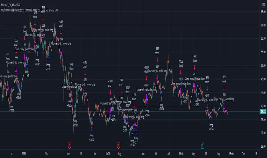
Swing Stock Market Multi MA Correlation This is a swing strategy adapted to stock market using correlation with either SP500 or Nasdaq, so its best to trade stocks from this region.
Its components are
Correlation Candle
Fast moving average to choose from SMA , EMA , SMMA (RMA), WMA and VWMA
Medium moving Average to choose from SMA , EMA , SMMA (RMA), WMA and VWMA
Slow moving average to choose from SMA , EMA , SMMA (RMA), WMA and VWMA
Rules for entry
Long: fast ma > medium ma and medium ma > slow ma
Short: fast ma< medium ma and medium ma < slow ma.
Rules for exit
We exit when we receive an inverse condition.
Caution:
This strategy use no risk management inside, so be careful with it .
If you have any questions, let me know !
+ JMA KDJ with RSI OB/OS SignalsSo, what is the KDJ indicator? If you're familiar with the Stochastic, then you'll know that the two oscillating lines are called the 'K' and 'D' lines. Now you know that this is some sort of implementation of the Stochastic. But, then, what is the J? The 'J' is simply the measure of convergence/divergence of the 'K' and 'D' lines, and the 'J' crossing the 'K' and 'D' lines is representational of the 'K' and 'D' lines themselves crossing. Is this an improvement over simply using the Stochastic as it is? Beats me. I don't use the Stochastic. I stumbled upon the KDJ while surfing around the web, and it sounded cool, so I thought I'd look at it. I do like it a bit more as the 'J' line being far overextended from the other two (usually into overbought/sold territory) does give a clear visual representation of the divergence of the 'K' and 'D' lines, which you might not notice otherwise. So, from that perspective I suppose it is nicer.
But let's get to the good stuff now, shall we? What did I do here?
Well, first thing you're wondering is why there are only two lines when based on my explanation (or your previous experience with the indicator) there should be three. I found this script here on TV, by x4random, who took the 'K' and 'D' lines and made an average of them, so there is only one line instead of the two. So, fewer lines on the indicator, but still the same usefulness. It was in older TV code, so I took it to version4 and cleaned up the code slightly. His indicator included the RSI ob/os plots, and I thought this was neat (even though the RSI being os/ob doesn't tell you much except that the trend is strong, and you should be buying pullback or selling rallies) so I kept them in. His indicator was also the most visually appealing one that I saw on here, so that attracted me too. Credit to x4random for the indicator, though.
Aside from code cleanup and adding the usual bells and whistles (which I will get to) the big thing I did here was change is RMA that he was using for the 'K' and 'D' lines to a Jurik MA's, which smooth a lot of the noise of other moving averages while maintaining responsiveness. This eliminates noise (false signals) while keeping the signals of significance. It took me a while to figure out how to substitute the JMA for the RMA, but thanks to QuantTherapy's "Jurik PPO" indicator I was able to nail down the implementation. One thing you might notice is that there is no input to change signal length. I fiddled with this for a time before sticking to using the period, instead of the signal (thus eliminating the use of the signal input altogether), length to generate the 'K' and 'D' calculations. To make any adjustments other than the period length use the Jurik Power input. You can use the phase input as well, but it has much less of an effect.
Everything else I changed is pretty much cosmetic.
Candle coloring with the option to color candles based on either the 'J' line or the 'KD' line.
color.from_gradients with color inputs to make it beautiful (this is probably my best looking indicator, imo)
plots for when crosses occur (really wish there was a way to plot these over candlesticks! If anyone has any suggestions I'd love to see!)
I think that's about it. Alerts of course.
Enjoy!
Below is a comparison chart of my JMA implementation to the original RMA script.
You can see how much smoother the JMA version is. Both of these had the default period of 55 set, and the JMA version is using the default settings, while the original version is using a length of 3 for the signal line.

Stochastic Momentum Index - SMI🎯 Overview
This is a Stochastic Momentum Index (SMI) indicator that combines stochastic momentum with moving average smoothing to identify trend direction and momentum strength in financial markets. The SMI measures where the current price closes relative to the midpoint of its recent trading range, providing enhanced sensitivity to price momentum.
🧩 Core Components
1. ⚙️ Technical Foundation
📊 Primary Calculation: Uses TradingView's built-in ta.stoch() function
📈 Range-Based: Compares closing price to high-low range over specified period
🎯 Scale: Oscillates between 0-100 with 50 as neutral midpoint
2. 🎛️ Configuration Parameters
📏 SMI Length: Default 101 periods (long-term smoothing)
📊 Source Price: Customizable (default = Close)
📈 MA Length: 30-period moving average applied to SMI
🔄 MA Type: 6 options (EMA, SMA, RMA, WMA, VWMA, HMA)
🎨 Color Themes: 5 visual schemes (Classic, Modern, Robust, Accented, Monochrome)
📈 Signal Interpretation:
🟢 BULLISH: SMI > 50 (price closing in upper half of range)
🔴 BEARISH: SMI < 50 (price closing in lower half of range)
🎯 Neutral Zone: Around 50 indicates balanced momentum
👁️ Visual Features
📈 Signal Line (MA):
Yellow moving average of SMI
Smooths momentum for clearer trend identification
🎯 Reference Lines:
50-level midpoint (white dashed line)
0-100 scale boundaries
🎨 Fill Zones:
🟢 Upper Zone : Bullish momentum area
🔴 Lower Zone : Bearish momentum area
Gradient fills enhance visual clarity
📋 Dashboard Display:
Content: "⬆️ Bullish" or "⬇️ Bearish" indicator
Purpose: Quick market bias assessment
⚡ Trading Applications
📈 Primary Uses:
🎯 Trend Identification
SMI > 50 = Uptrend momentum
SMI < 50 = Downtrend momentum
📊 Momentum Strength
Values near 100 = Strong bullish momentum
Values near 0 = Strong bearish momentum
Values around 50 = Neutral/consolidation
🔄 Mean Reversion
Extreme readings (near 0 or 100) may indicate overbought/oversold conditions
⏰ Timeframe Compatibility:
📅 Long-term: 101-period default suits swing/position trading
📊 Medium-term: Adjust lengths for daily/weekly analysis
⚡ Short-term: Reduce periods for intraday trading
🎨 Customization Options
🔄 Moving Average Types:
📉 EMA: Exponential - responsive to recent changes
📊 SMA: Simple - equal weight to all periods
📈 RMA: Relative - TradingView's special moving average
⚖️ WMA: Weighted - emphasizes recent data
💎 VWMA: Volume-weighted - incorporates volume
🚀 HMA: Hull - reduces lag significantly
🎨 Visual Themes:
🎨 Classic: Green/Red (traditional trading colors)
🚀 Modern: Cyan/Purple (modern aesthetic)
💪 Robust: Amber/Deep Purple (high contrast)
🌈 Accented: Purple/Magenta (vibrant)
⚫⚪ Monochrome: Light Gray/Dark Gray (minimalist)
🔔 Alert System
🟢 LONG Alert: Triggers when SMI crosses above 50
🔴 SHORT Alert: Triggers when SMI crosses below 50
📧 Format: Includes ticker symbol for easy identification
⚡ Key Advantages
✅ Strengths:
🎯 Clear Signals: Simple >50/<50 threshold for easy interpretation
📊 Range-Bound: Always oscillates 0-100 (no divergence issues)
👁️ Visual Clarity: Color-coded zones make analysis intuitive
🔄 Customizable: Multiple MA types and visual themes
📱 Professional: Clean, organized display suitable for all traders

Momentum RSIMomentum RSI (MRSI | MisinkoMaster)
Momentum RSI is an enhanced version of the classic Relative Strength Index (RSI) developed by J. Welles Wilder. This indicator integrates momentum components directly into the RSI calculation, resulting in a faster, smoother oscillator that helps traders identify trend strength and value zones with greater precision.
Unlike the traditional RSI, which relies on a fixed smoothing approach, the Momentum RSI dynamically incorporates momentum derived from differences between moving averages of RSI values over different lookback periods. This improves signal responsiveness while reducing noise, providing clearer insights for both trend-following and mean-reversion trading strategies.
🔍 Concept & Idea
Momentum RSI aims to improve the original RSI by adding momentum elements that speed up its reaction to price changes without sacrificing smoothness. This hybrid approach helps:
Capture early signals in trending markets
Reduce false signals during sideways or choppy conditions
Highlight overbought and oversold zones more effectively
Provide additional momentum context for more informed trading decisions
By combining RSI with momentum derived from moving average differences, the indicator balances sensitivity and stability for a versatile application across different asset classes and timeframes.
⚙️ How It Works
The Momentum RSI calculation involves several key steps:
Standard RSI Calculation:
The indicator first calculates the classic RSI using user-defined length and smoothing parameters. Users can customize the RSI source price and the smoothing moving average (MA) type applied (options include RMA, SMA, EMA, WMA, DEMA, TEMA, HMA, ALMA).
Momentum Derivation:
Two versions of the RSI are computed with different smoothing lengths—a base RSI and a longer smoothed RSI. The difference between their moving averages represents a momentum component that measures the short-term trend strength.
Additional Momentum:
The difference between shorter-length and longer-length RSI calculations adds another momentum layer, reflecting momentum shifts over different timescales.
Momentum Integration:
These momentum components are combined and added to the previous RSI value, resulting in a momentum-enhanced RSI value (mrsi) that oscillates between 0 and 100.
Trend Detection:
Customizable upper and lower thresholds define long and short signal zones, allowing users to interpret when the market is trending bullish or bearish.
Overbought/Oversold Zones:
Additional thresholds highlight extreme value zones for potential mean-reversion trades.
🧩 Inputs Overview
RSI Length - Controls the primary RSI calculation length (default 20).
Source - Selects the price source for the RSI calculation (default: close).
Smoothing Length - Length used to smooth RSI values with the chosen MA type (default 12).
MA Type - Moving average method used for smoothing (options: RMA, SMA, EMA, WMA, DEMA, TEMA, HMA, ALMA).
ALMA Offset - Offset parameter for ALMA smoothing (applicable only if ALMA is selected).
ALMA Sigma - Sigma parameter for ALMA smoothing (applicable only if ALMA is selected).
Upper Threshold - RSI level above which a bullish (long) signal is triggered (default 55).
Lower Threshold - RSI level below which a bearish (short) signal is triggered (default 45).
Overbought Threshold - RSI level indicating overbought conditions (default 85).
Oversold Threshold - RSI level indicating oversold conditions (default 15).
📌 Usage Notes
Versatile Application: Use Momentum RSI for both trend-following and mean-reversion strategies.
Signal Clarity: The momentum integration reduces noise, helping avoid false breakouts and improving entry timing.
Customization: Adjust smoothing lengths and MA types to match the characteristics of your trading style or the specific asset.
Visual Aids: Background colors, candle coloring, and shape markers facilitate quick interpretation of momentum strength and trend changes.
Threshold Sensitivity: Fine-tune thresholds to balance between early signals and signal reliability.
Intrabar Updates: Signals may update on lower timeframes for responsive trading.
Combine with Other Tools: For best results, use Momentum RSI alongside volume, price action, or other confirmation indicators.
Backtest Before Live Trading: Always validate settings on historical data to ensure suitability for your trading instrument and timeframe.
⚠️ Disclaimer
This script is intended for educational and analytical purposes only and does not constitute financial advice. Trading involves risk, and users should perform their own due diligence before making any trading decisions.

Moving Average Exponential//@version=6
indicator(title="Moving Average Exponential", shorttitle="EMA", overlay=true, timeframe="", timeframe_gaps=true)
len = input.int(9, minval=1, title="Length")
src = input(close, title="Source")
offset = input.int(title="Offset", defval=0, minval=-500, maxval=500, display = display.data_window)
out = ta.ema(src, len)
plot(out, title="EMA", color=color.blue, offset=offset)
// Smoothing MA inputs
GRP = "Smoothing"
TT_BB = "Only applies when 'SMA + Bollinger Bands' is selected. Determines the distance between the SMA and the bands."
maTypeInput = input.string("None", "Type", options = , group = GRP, display = display.data_window)
var isBB = maTypeInput == "SMA + Bollinger Bands"
maLengthInput = input.int(14, "Length", group = GRP, display = display.data_window, active = maTypeInput != "None")
bbMultInput = input.float(2.0, "BB StdDev", minval = 0.001, maxval = 50, step = 0.5, tooltip = TT_BB, group = GRP, display = display.data_window, active = isBB)
var enableMA = maTypeInput != "None"
// Smoothing MA Calculation
ma(source, length, MAtype) =>
switch MAtype
"SMA" => ta.sma(source, length)
"SMA + Bollinger Bands" => ta.sma(source, length)
"EMA" => ta.ema(source, length)
"SMMA (RMA)" => ta.rma(source, length)
"WMA" => ta.wma(source, length)
"VWMA" => ta.vwma(source, length)
// Smoothing MA plots
smoothingMA = enableMA ? ma(out, maLengthInput, maTypeInput) : na
smoothingStDev = isBB ? ta.stdev(out, maLengthInput) * bbMultInput : na
plot(smoothingMA, "EMA-based MA", color=color.yellow, display = enableMA ? display.all : display.none, editable = enableMA)
bbUpperBand = plot(smoothingMA + smoothingStDev, title = "Upper Bollinger Band", color=color.green, display = isBB ? display.all : display.none, editable = isBB)
bbLowerBand = plot(smoothingMA - smoothingStDev, title = "Lower Bollinger Band", color=color.green, display = isBB ? display.all : display.none, editable = isBB)
fill(bbUpperBand, bbLowerBand, color= isBB ? color.new(color.green, 90) : na, title="Bollinger Bands Background Fill", display = isBB ? display.all : display.none, editable = isBB)

Multi-Sigma Bands [fmb]Multi-Sigma Bands plots standard deviation (sigma) bands around a selectable basis (SMA, EMA, RMA, or Linear Regression). It’s designed to help you spot when price is behaving “normally” versus when it’s stretching into statistically extended territory.
What it shows
- Basis: the central reference line (your chosen basis type)
- ±1σ zone: the common range where price spends much of its time
- ±2σ zone: extended range where moves often become more emotional or trend-driven
- ±3σ zone: extreme range where price is statistically stretched (risk increases)
How to read it
- Inside ±1σ
- Often normal behaviour and mean-reverting price action around the basis.
- Between ±1σ and ±2σ
- A meaningful extension. In trends, price can “walk” these areas for longer than expected.
- Between ±2σ and ±3σ
- Rare extension. Can signal exhaustion, blow-off behaviour, or capitulation depending on direction and context.
How traders typically use it
- Trend context
- In strong uptrends, price may ride the upper bands (+1σ to +2σ) repeatedly.
- In strong downtrends, the lower bands (-1σ to -2σ) can act the same way.
- Bands show statistical stretch, not automatic reversal signals.
- Extension and risk framing
- The farther price is from the basis, the more “stretched” it is.
- That usually means chasing becomes riskier and entries require tighter confirmation.
- Range behaviour
- Ranges often oscillate around the basis, with frequent returns toward the middle zone.
Settings
- Source: what price series to use (Close by default)
- Length: lookback used for both basis and standard deviation
- Basis: SMA, EMA, RMA, or LinReg
- Stdev smoothing: optional smoothing on standard deviation for cleaner bands
- σ multipliers: customise σ1, σ2, σ3 (defaults: 1, 2, 3)
- Force Monthly Data (optional): calculate bands using a higher-timeframe source to reduce noise and focus on macro structure
Disclaimer
This indicator is for informational and educational purposes only and is not financial advice. Always use risk management and confirm with market structure and trend context.

Luminous Volume Flow [Pineify]Luminous Volume Flow
The Luminous Volume Flow is a specialized volume-based momentum oscillator designed to uncover the underlying buying and selling pressure within the market. Unlike traditional volume indicators that simply aggregate volume based on the close relative to the open, LVF analyzes intrabar dynamics—specifically the relationship between the close price and the high/low wicks—to estimate the dominance of buyers or sellers.
By smoothing this raw volume delta and applying a signal line, the LVF provides a clear visual representation of volume flow, helping traders identify trend strength, potential reversals, and momentum shifts with high-definition "luminous" visuals.
Key Features
Intrabar Pressure Analysis : Calculates buying and selling pressure based on wick dynamics and price polarity to provide a more granular view of market sentiment.
Multi-Type Smoothing : Offers selectable Moving Average types (SMA, EMA, RMA) for the main Flow Line to adapt to different market volatilities.
Luminous Visuals : Utilizes dynamic color gradients that brighten as momentum expands and darken as it contracts, offering immediate visual feedback on trend intensity.
Sentiment Cloud : Fills the area between the Flow and Signal lines to clearly visualize the prevailing bullish or bearish sentiment.
High-Contrast Signals : Optional high-contrast signal markers for clear crossover identification.
How It Works
The LVF operates on a multi-stage calculation process:
Pressure Calculation : The script compares the lower wick (Close - Low) against the upper wick (High - Close).
If the lower wick is longer, it suggests buying pressure (rejection of lower prices), and volume is assigned to Buy Pressure .
If the upper wick is longer, it suggests selling pressure (rejection of higher prices), and volume is assigned to Sell Pressure .
If equal, the Close > Open polarity is used as a tie-breaker.
Raw Delta : The difference between Buy and Sell Pressure is calculated to determine the net volume flow for the bar.
Flow Line : The Raw Delta is smoothed using a user-selected Moving Average (SMA, EMA, or RMA) over the Flow Length period. This creates the main oscillator line.
Signal Line : An EMA of the Flow Line is calculated to generate the Signal Line, similar to the MACD mechanic.
Histogram : The difference between the Flow Line and Signal Line determines the Histogram, which drives the "Luminous" color gradient logic.
Trading Ideas and Insights
Trend Confirmation : When the Flow Line is above the Signal Line and the Cloud is green, the bullish trend is supported by volume. Conversely, a red cloud indicates bearish volume dominance.
Momentum Crossovers : The triangle shapes indicate crossovers between the Flow and Signal lines. A triangle up (Green) suggests a potential bullish entry or invalidation of a short bias. A triangle down (Red) suggests a bearish turn.
Expansion vs. Contraction : Pay attention to the brightness of the histogram columns. Bright colors indicate expanding momentum (a strong move), while darker, fading colors suggest the move is losing steam, potentially preceding a consolidation or reversal.
How multiple components work together
This script combines the logic of Volume Delta analysis with Signal Line Crossover mechanics (popularized by MACD). By applying trend-following smoothing to raw volume data, we transform erratic volume spikes into a coherent flow. The "Luminous" visual layer is added to make the data interpretation intuitive—removing the need to mentally calculate the rate of change based on histogram height alone.
Unique Aspects
Adaptive Gradient Coloring : The histogram doesn't just show positive/negative values; it visually communicates the *acceleration* of the move via color intensity based on standard deviation.
Wick-Based Volume Attribution : Instead of a binary close-to-open comparison, LVF respects the price action within the candle (the wicks), acknowledging that a long lower wick on a red candle can actually represent significant buying interest.
How to Use
Add the indicator to your chart.
Adjust the Flow Length to match your trading timeframe (lower for scalping, higher for swing trading).
Select your preferred Smoothing Type (EMA is default and recommended for responsiveness).
Use the "Sentiment Cloud" filter: Look for long signals only when the cloud is green, and short signals when the cloud is red.
Monitor the Luminous Histogram for signs of exhaustion (colors fading) to manage exits.
Customization
Flow Length : Period for the main smoothing (Default: 14).
Signal Length : Period for the signal line (Default: 9).
Smoothing Type : Choose between SMA, EMA, or RMA.
Colors : Fully customizable colors for Bullish/Bearish phases and signals.
Chart Bars : Option to color the main chart candles based on the Flow direction.
Conclusion
The Luminous Volume Flow is a robust tool for traders who want to go beyond price action and understand the volume dynamics driving the market. By visualizing the flow of buying and selling pressure with advanced smoothing and reactive visuals, it provides a clearer picture of market sentiment than standard volume bars.

Institutional Alpha Vector | D_QUANT Institutional Alpha Vector | D_QUANT
Overview
The Institutional Alpha Vector (IAV) is an original trend-following framework that replaces single-indicator bias with a Weighted Composite Score . Instead of relying on a simple moving average, this script aggregates four distinct quantitative dimensions—Price, Momentum, Volatility, and Volume—into a normalized value called the "Alpha Vector."
The goal of this tool is to identify "Institutional Consensus"—periods where multiple mathematical models align in the same direction, reducing the likelihood of false breakouts in choppy markets.
How It Works: The Quantitative Engines
The script calculates four independent signals. For each module, a state is stored (1 for Bullish, -1 for Bearish, 0 for Neutral).
1. Price Filter (Hull Moving Average):
The script uses an HMA (a weighted moving average that reduces lag by using the square root of the period). A signal is triggered when the price crosses over/under this "Spine."
2. Volatility Regime (RMA + ATR):
This module uses a Moving Average (RMA) combined with an Average True Range (ATR) offset. It acts as a volatility filter that price must move beyond 1 ATR from the mean to register a trend, ensuring the market isn't just "drifting."
3. Momentum Physics (ADX/DMI):
Based on J. Welles Wilder’s Directional Movement Index. It checks if the is above (or vice versa) but only if the ADX (Average Directional Index) is above a user-defined threshold (default: 10), confirming the presence of a strong trend.
4. Institutional Flow (Chaikin Money Flow):
This confirms price action with volume. It calculates the accumulation/distribution of money flow over a specific period. A signal is only valid if the CMF is positive (Bullish) or negative (Bearish).
The Alpha Vector Calculation
This is the core "originality" of the script. The indicator takes the active modules and calculates a Composite Score :
This results in a value between -1.0 and +1.0 .
* High Confidence Long: When the score exceeds +0.1 (adjustable).
* High Confidence Short: When the score drops below -0.1 (adjustable).
* Neutral Zone: When the score is near 0, the script colors the bars grey, signaling a lack of institutional consensus.
Visual Intelligence: The "Electric Conduit"
The script visualizes market energy through a custom rendering engine:
* The Spine: A central line representing the HMA trend.
* The Conduit (Fill): A dynamic gradient that expands or contracts based on the ATR (Average True Range) . This allows traders to see "volatility expansion" (wide ribbon) vs "compression" (tight ribbon) at a glance.
* Bar Coloring : Automatically aligns the chart candles with the Alpha Vector state to remove cognitive load.
How to Use
1. Define your Strategy: In the settings, you can toggle specific modules. If you are trading a low-volume asset, you might disable the **CMF** module.
2. Identify the Consensus: Look for the ribbon to change from Grey (Neutral) to Cyan/Gold.
3. Monitor the HUD: A small dashboard in the bottom right displays the live Alpha Vector score. A score of 1.0 means all four engines are in 100% bullish agreement.
Disclaimer: Trading involves significant risk. This tool is for educational and analytical purposes and does not constitute financial advice.

SuperRSI: Enhanced MomentumTitle: SuperRSI: Enhanced Momentum
Description:
Overview The SuperRSI is not your standard Relative Strength Index. While traditional RSI calculates momentum based solely on close prices, this "Titan Edition" incorporates price structure breakouts. It analyzes whether the price is breaking new highs or lows within the lookback period to calculate momentum. This makes the SuperRSI significantly more responsive to volatility and genuine market action than the classic formula.
Key Features
Titan Calculation Logic: Uses High/Low breakouts to capture true momentum, making it faster and more sensitive than standard RSI.
Dynamic Trend Coloring: The RSI line automatically changes color to give you an instant visual bias:
Green: RSI is above the Signal Line (Bullish Momentum).
Red: RSI is below the Signal Line (Bearish Momentum).
Signal Line Filtering: Includes a built-in "Slow Signal" (EMA based) to help filter out market noise and identify sustainable trends.
Visual Gradients: Clear background fills for Overbought (OB) and Oversold (OS) zones to highlight extreme conditions.
How to Use
Trend Identification: Simply look at the line color. If it’s Green, momentum is bullish. If it’s Red, momentum is bearish.
Entry & Exit Signals: Watch for the crossover between the RSI line and the Signal Line. A cross above is a buy signal; a cross below is a sell signal.
Overbought/Oversold:
Above 80: Extreme bullish momentum (potential reversal or strong trend continuation).
Below 20: Extreme bearish momentum.
Settings
Fully customizable lengths for RSI and Signal lines.
Adjustable Smoothing methods (RMA, SMA, EMA).
Customizable Overbought/Oversold levels (Default: 80/20)
العنوان: SuperRSI: Enhanced Momentum
الوصف:
نظرة عامة مؤشر SuperRSI ليس مجرد مؤشر قوة نسبية تقليدي. بينما يعتمد الـ RSI العادي على أسعار الإغلاق فقط، تعتمد هذه النسخة المطور (Titan Edition) على اختراقات الهيكل السعري. يقوم المؤشر بحساب الزخم بناءً على ما إذا كان السعر يكسر قمماً جديدة أو قيعانًا جديدة خلال الفترة المحددة. هذا يجعله أكثر استجابة للتقلبات وحركة السوق الحقيقية مقارنة بالمعادلة الكلاسيكية.
أهم المميزات
معادلة Titan للزخم: تستخدم اختراقات القمم والقيعان (High/Low) لالتقاط الزخم الحقيقي، مما يجعله أسرع وأدق من RSI العادي.
تلوين ديناميكي للاتجاه: يتغير لون خط المؤشر تلقائياً ليعطيك رؤية فورية للاتجاه:
اللون الأخضر: الـ RSI يتداول فوق خط الإشارة (زخم صاعد).
اللون الأحمر: الـ RSI يتداول تحت خط الإشارة (زخم هابط).
فلترة الإشارات: يحتوي على "خط إشارة" مدمج (Slow Signal) لتنقية ضجيج السوق (Noise) وتحديد الاتجاهات المستدامة.
تدرجات لونية: خلفيات واضحة لمناطق التشبع الشرائي (Overbought) والتشبع البيعي (Oversold).
طريقة الاستخدام
تحديد الاتجاه: انظر ببساطة إلى لون الخط. إذا كان أخضر فالزخم شرائي، وإذا كان أحمر فالزخم بيعي.
إشارات الدخول والخروج: راقب التقاطع بين خط الـ RSI وخط الإشارة. التقاطع لأعلى يعتبر إشارة شراء، والتقاطع لأسفل يعتبر إشارة بيع.
مناطق التشبع:
فوق 80: تشبع شرائي (احتمالية انعكاس أو استمرار قوي للترند).
تحت 20: تشبع بيعي.
الإعدادات
إمكانية تعديل المدة الزمنية (Length) للـ RSI وخطوط الإشارة.
خيارات متعددة لنوع المتوسط المستخدم (RMA, SMA, EMA).
مستويات تشبع قابلة للتعديل (الافتراضي: 80/20).

FxInside// This Pine Script® code is subject to the terms of the Mozilla Public License 2.0 at mozilla.org
// © yyy_trade
//@version=6
indicator("FxInside", overlay = true, max_lines_count = 500)
lineColor = input.color(color.new(color.blue, 12), "FxLineColor")
type vaild_struct
float high
float low
int time
type fx
string dir
chart.point point
var array valid_arr = array.new()
var fx lastFx = na
var float motherHigh = na
var float motherLow = na
isInsideBar = high <= high and low >= low
if isInsideBar and na(motherHigh)
motherHigh := high
motherLow := low
isExtendedInsideBar = not na(motherHigh) and high <= motherHigh and low >= motherLow
body_color = input.color(color.new(color.orange, 0), "实体颜色")
wick_color = input.color(color.new(color.orange, 0), "影线颜色")
border_color = input.color(color.new(color.orange, 0), "边框颜色")
plotcandle(open, high, low, close, color=isExtendedInsideBar ? body_color : na, wickcolor=isExtendedInsideBar ? wick_color : na, bordercolor =isExtendedInsideBar ? border_color : na ,editable=false)
if not na(motherHigh) and (high > motherHigh or low < motherLow)
motherHigh := na
motherLow := na
// 以下为分型折线逻辑,如不需要可删除
process_fx(last_fx, now_fx) =>
if not na(last_fx)
line.new(last_fx.point, now_fx.point, color=lineColor, xloc=xloc.bar_time)
now_fx
if not isExtendedInsideBar
array.push(valid_arr, vaild_struct.new(high, low, time))
if array.size(valid_arr) > 17
array.shift(valid_arr)
len = array.size(valid_arr)
if len > 3
k_ago = array.get(valid_arr, len - 2)
k_now = array.get(valid_arr, len - 1)
if k_ago.high > k_now.high
for i = 3 to len
last_k = array.get(valid_arr, len - i)
if last_k.high < k_ago.high
if last_k.low < k_ago.low
lastFx := process_fx(lastFx, fx.new("TOP", chart.point.from_time(k_ago.time, k_ago.high)))
break
else
if not na(lastFx)
if lastFx.dir == "TOP"
lastFx := process_fx(lastFx, fx.new("BOT", chart.point.from_time(last_k.time, last_k.low)))
lastFx := process_fx(lastFx, fx.new("TOP", chart.point.from_time(k_ago.time, k_ago.high)))
break
else if last_k.high > k_ago.high
break
// 底分型判定
if k_ago.low < k_now.low
for i = 3 to len
last_k = array.get(valid_arr, len - i)
if last_k.low > k_ago.low
if last_k.high > k_ago.high
lastFx := process_fx(lastFx, fx.new("BOT", chart.point.from_time(k_ago.time, k_ago.low)))
break
else
if not na(lastFx)
if lastFx.dir == "BOT"
lastFx := process_fx(lastFx, fx.new("TOP", chart.point.from_time(last_k.time, last_k.high)))
lastFx := process_fx(lastFx, fx.new("BOT", chart.point.from_time(k_ago.time, k_ago.low)))
break
else if last_k.low < k_ago.low
break
len = input.int(20, minval=1, title="Length")
src = input(close, title="Source")
offset = input.int(title="Offset", defval=0, minval=-500, maxval=500, display = display.data_window)
out = ta.ema(src, len)
plot(out, title="EMA", color=color.blue, offset=offset)
// Smoothing MA inputs
GRP = "Smoothing"
TT_BB = "Only applies when 'SMA + Bollinger Bands' is selected. Determines the distance between the SMA and the bands."
maTypeInput = input.string("None", "Type", options = , group = GRP, display = display.data_window)
maLengthInput = input.int(14, "Length", group = GRP, display = display.data_window)
bbMultInput = input.float(2.0, "BB StdDev", minval = 0.001, maxval = 50, step = 0.5, tooltip = TT_BB, group = GRP, display = display.data_window)
var enableMA = maTypeInput != "None"
var isBB = maTypeInput == "SMA + Bollinger Bands"
// Smoothing MA Calculation
ma(source, length, MAtype) =>
switch MAtype
"SMA" => ta.sma(source, length)
"SMA + Bollinger Bands" => ta.sma(source, length)
"EMA" => ta.ema(source, length)
"SMMA (RMA)" => ta.rma(source, length)
"WMA" => ta.wma(source, length)
"VWMA" => ta.vwma(source, length)
// Smoothing MA plots
smoothingMA = enableMA ? ma(out, maLengthInput, maTypeInput) : na
smoothingStDev = isBB ? ta.stdev(out, maLengthInput) * bbMultInput : na
plot(smoothingMA, "EMA-based MA", color=color.yellow, display = enableMA ? display.all : display.none, editable = enableMA)
bbUpperBand = plot(smoothingMA + smoothingStDev, title = "Upper Bollinger Band", color=color.green, display = isBB ? display.all : display.none, editable = isBB)
bbLowerBand = plot(smoothingMA - smoothingStDev, title = "Lower Bollinger Band", color=color.green, display = isBB ? display.all : display.none, editable = isBB)
fill(bbUpperBand, bbLowerBand, color= isBB ? color.new(color.green, 90) : na, title="Bollinger Bands Background Fill", display = isBB ? display.all : display.none, editable = isBB)

Price Action TrendPrice Action Trend measures trend *strength* by modelling where price sits inside a smoothed price-action channel, then applying RSI to that “channel position”. It doesn’t predict, but shows what price is doing now.
This indicator uses the same calculations as my old "Price Action Trend Overlay" script, which I'd published Protected for some forgotten reason. Some users have asked for the source code, so I'm republishing it as open source. I've also tidied up the code a bit, added some visualisations of elements that were present but never drawn, such as the PA channels themselves, drawn the trend metric in a separate pane, added alerts, and made some more configuration options available.
🟩 HIGHLIGHTS
⭐ Trend colouring on the main chart.
⭐ A trend line drawn in its own pane.
⭐ Overbought/oversold markers on the main chart, derived from the same PA calculations.
⭐ Optional “Price Average” line and channel colouring.
🟩 WHAT’S UNIQUE ABOUT THE TREND CALCULATION
Most “trend RSI” tools run RSI on close, or on some moving average of price.
This script runs RSI on a *normalised* price-action series:
- We build a smoothed channel from RMA(high) and RMA(low).
- We normalise price against that channel (relative to the channel midpoint and width).
- We run RSI on that normalised series (default 14, but optionally matched to the Trend Lookback Period).
Using highs and lows instead of close or OHLC4 makes the trend value sensitive to *range shape* and *asymmetry* (big wicks, uneven extremes), not just the centre of the candle.
As compared to a simple RSI (also included simply for comparison), this PA Trend tends to decay faster and recovers faster.
🟩 HOW TO USE IT (PRACTICAL)
⭐ Trend pane
- Treat the line as a measure of *trend strength*, not a prediction.
- Neutral zone = trend is not convincingly bullish or bearish.
- Strong moves away from neutral = “trend has conviction”.
⭐ Overbought / oversold markers
Overbought/oversold doesn’t mean “reversal right now”.
It means the *rate of directional change* is unsustainably strong.
- Overbought in an uptrend: trend is overheating. Tighten long stops; expect rest/retrace/reversal once overheating ends.
- Oversold in an uptrend: the countertrend down is likely exhausting. Potential “buy the dip” context.
- Reverse the above for downtrends.
This works on any market, any timeframe. Lower timeframes will be choppier.
Don’t trade these signals blindly; use market structure, S/R, and your other tools.
🟩 SETTINGS (OVERVIEW)
🟦 Settings
- Pane Plot Mode: choose whether the pane shows Trend or Overbought/Oversold series.
- Trend Lookback Period: channel smoothing for the trend model (higher = smoother, lower = faster).
- Show Overbought & Oversold Shapes: show/hide the triangles on the main chart.
- Overbought/sold Lookback Period: channel smoothing for OB/OS detection (lower = more sensitive).
- Overbought/sold Adaptive Length: smoothing for the dynamic OB/OS levels (lower = more adaptive).
🟦 Display
- Transparency for the candle colour: bar colour transparency (Gradient mode).
- Trend Colour Mode: Classic vs strength-based Gradient.
🟦 Price Average
- Show Price Average: show/hide the OHLC4 average price line.
- Lookback: length for the price average.
- Smoothing: SMA / EMA / RMA.
- Colour Channel by Price Average: neutral/green/red channel colouring depending on whether the price average is inside/above/below the channel.
🟦 Advanced
- Trend Upper/Lower Neutral Threshold: neutral zone bounds (also used by the dynamic OB/OS logic).
- PA RSI Length: choose Fixed (14) or match the Trend Lookback Period.
- Show RSI (close): optional “reference RSI” plot with length.
🟩 ALERTS
There are built-in alert conditions for this indicator:
- Overbought PA Trend: triggers when the PA overbought condition is true.
- Oversold PA Trend: triggers when the PA oversold condition is true.
- Trend flips up: triggers when the trend changes from down to up (ignores any intervening neutral bars).
- Trend flips down: triggers when the trend changes from up to down (ignores any intervening neutral bars).
- Lost overbought: triggers on the first red candle after the overbought condition ends (set this alert on close to avoid false alerts).
- Lost oversold: triggers on the first green candle after the oversold condition ends (set this alert on close to avoid false alerts).
🟩 REPAINTING / CALCULATION NOTES
According to my understanding, this indicator does not repaint (it does not go back and alter closed bars).
However, while the current candle is forming, values that depend on the current price will update in real time. Once the candle closes, they are fixed.
The overbought/oversold calculations use Williams fractal-style confirmation logic, which cannot be known until some bars afterwards.
This affects when the OB/OS levels update, but new confirmations only affect future calculations, not the past.
🟩 CREDITS
The idea for using smoothed highs/lows to create a price-action channel came from my humble trading mentor. All the code is my own.
🟩 DISCLAIMER
No indicator is a substitute for knowing what you’re doing.
By using this indicator you agree that it might not do what you or anyone else expects.
You retain full responsibility for your trading at all times.
Before trading with actual money, first make sure your risk management is professional-level.

Supertrend BUY Only - Optimized for Gold M15 TimeframeOverview
The Supertrend BUY Only - Production Optimized is a high-performance trend-following indicator specifically tuned for XAUUSD (Gold) on the 15-minute timeframe. Unlike standard Supertrend scripts, this version focuses exclusively on bullish cycles to align with long-term upward bias and uses parameters discovered through deep data analysis of over 20,000 bars of historical market data.
Key Features
Data-Optimized Parameters: Defaults are set to ATR Period 7 and Multiplier 2.1, which backtesting has shown to provide a superior balance between sensitivity and noise reduction for Gold.
Production-Ready Alerts: Includes built-in alertcondition triggers for both BUY (Trend Flip) and STOP BUY (Trend Exit), complete with dynamic messages that include price and interval.
Trailing Support Band: Uses a trailing logic that locks in support levels during upward moves, preventing the band from dropping until the trend officially reverses.
Clean Visuals: Focuses on chart clarity by only plotting the support line during active uptrends and utilizing clean shape labels for entries and exits.
How to Use
Entry (BUY): When the Supertrend line flips from Red to Green and a "BUY" label appears. This indicates bullish momentum has overcome recent volatility.
Exit (STOP BUY): When the price closes below the Green support line. The indicator will plot a red "X" and clear the green background.
Setting Alerts: * Click the Alerts icon in TradingView.
Select this indicator under "Condition."
Choose "BUY Signal" for entries and "STOP BUY / EXIT" for managing your trade or taking profit.
Technical Details
The script allows users to toggle between the TradingView (RMA) ATR calculation and the Standard (SMA) method. For production and live trading, the RMA method is recommended as it provides a smoother response to volatility spikes common in the Gold market.

Adaptive Strength Overlay (MTF) [BackQuant]Adaptive Strength Overlay (MTF)
A multi-timeframe RSI strength visualizer that projects oscillator “pressure” directly onto price using adaptive gradient fills between percent bands. Built to make strength, exhaustion, and regime context readable at a glance, without needing to stare at a separate oscillator panel.
Mean-Reversion mode example
What this indicator does
This indicator converts RSI strength into a chart overlay that reacts to momentum and extremes, then visualizes it as colored “pressure zones” around price.
Instead of plotting RSI in a sub-window, it:
Builds 1 to 3 symmetric percent bands above and below price.
Computes RSI strength on up to 3 different timeframes (MTF).
Smooths RSI with your selected moving average type.
Maps RSI values into discrete transparency “buckets”.
Fills between the bands with a gradient whose opacity reflects strength or exhaustion.
Displays a compact RSI table for all enabled timeframes.
Provides alert conditions for extremes and midline shifts on each timeframe.
The result is an overlay that looks like a dynamic envelope. When strength rises, the envelope “lights up” in the direction of the move. When strength becomes stretched, the outer zones become visually prominent.
Core idea: “Strength as an overlay”
RSI is normally interpreted in a separate oscillator panel. That makes context-switching slow:
You check price action.
You look down at RSI.
You mentally translate RSI into risk or trend bias.
This script removes that translation step by projecting strength directly onto the price area, using band fills as a visual language:
More visible fill = stronger strength or more extreme condition (depending on mode).
Less visible fill = weak strength or neutral state.
Two operating modes
1) Trend mode
Trend mode emphasizes strength aligned with direction:
When RSI is strong on the upside, upper bands become more visible.
When RSI is strong on the downside, lower bands become more visible.
Neutral RSI fades, so the chart de-clutters during chop.
Use Trend mode when:
You want a clean trend-following overlay.
You want to quickly see which timeframe(s) are powering the move.
You want to filter entries to moments when strength confirms direction.
2) Mean-Reversion mode
Mean-Reversion mode flips the emphasis to highlight exhaustion against the move :
Upper extremes become a “potential exhaustion” cue.
Lower extremes become a “potential exhaustion” cue.
The overlay is tuned to make stretched conditions obvious.
This is not an automatic “short overbought / long oversold” system. It is a visualization mode that makes “extended” conditions stand out faster, especially when multiple timeframes align.
How the bands work (Percent Bands)
The indicator constructs up to three symmetric envelopes around price:
Band 1: percent1 scaled by scale
Band 2: percent2 scaled by scale (optional)
Band 3: percent3 scaled by scale (optional)
The percent bands are simple deviations from the selected price source:
Upper = price * (1 + (percent * scaling)/100)
Lower = price * (1 - (percent * scaling)/100)
Why this matters:
It anchors “strength visualization” to meaningful price distance.
It makes the overlay comparable across assets because it’s percent-based.
It gives you a consistent spatial frame for reading momentum versus extension.
Multi-timeframe engine (MTF)
The script runs the same strength calculation on up to three timeframes:
Timeframe 1 uses the chart timeframe by default (empty string input).
Timeframe 2 is optional and defaults to Daily.
Timeframe 3 is optional and defaults to Weekly.
Each timeframe has:
Its own RSI period (len, len2, len3).
Its own smoothing length (slen, slen2, slen3).
The same smoothing type selection (EMA, HMA, etc).
This creates a layered view:
TF1 often reflects tactical pressure (entries/exits).
TF2 reflects structural pressure (swing context).
TF3 reflects macro bias (regime context).
When multiple timeframes agree, the fills stack and the overlay becomes visually louder. When they disagree, the overlay looks mixed or muted, which is exactly the point.
Smoothing options (why so many)
Raw RSI can be noisy. This script lets you smooth RSI with multiple MA types, which changes how “responsive” the overlay feels:
EMA/RMA smooth without lagging as hard as SMA.
HMA responds faster but can be twitchy.
LINREG can feel more “structural”.
ALMA and T3/TEMA provide heavier smoothing profiles with different lag characteristics.
This isn’t cosmetic. Your smoothing choice affects:
How early the overlay “lights up” in Trend mode.
How long extremes remain highlighted in Mean-Reversion mode.
How often fills flicker in chop.
Strength mapping (the transparency buckets)
Instead of mapping RSI to a continuous color scale, the script uses a discrete transparency ladder. That creates a clean, readable visual that avoids constant flickering.
The logic assigns two transparency values per timeframe:
Upper-side transparency responds to lower RSI zones (weak upside strength).
Lower-side transparency responds to higher RSI zones (strong upside strength).
Then the script uses those transparencies differently depending on mode:
Trend mode shows “strength aligned with direction”.
Mean-Reversion mode swaps the emphasis so “extremes” stand out as potential stretch.
You can think of it as:
Trend mode highlights continuation strength.
Mean-Reversion mode highlights potential exhaustion.
Fill stacking (how the overlay is built)
The overlay uses layered fills:
Fill from price to Band 1
Fill from Band 1 to Band 2 (if enabled)
Fill from Band 2 to Band 3 (if enabled)
Upper side uses the negative color (typically red) and lower side uses the positive color (typically green), because upper bands represent “above price” space and lower bands represent “below price” space. The intensity is controlled by the computed transparency per timeframe and selected mode.
Important behavior:
Disabling Band 2 or Band 3 can change how the stacked fills look, because you are removing fill segments.
If you want a clean look, run only Band 1.
If you want a “regime heat” look, run Bands 1–3 with higher scaling.
Table (MTF RSI dashboard)
A compact table prints RSI values for each configured timeframe:
Row labels show TF.
Values show the smoothed RSI output that drives the overlay.
Use it for quick confirmation:
If overlay looks strong but table RSI is neutral, your band settings might be too tight.
If TF3 RSI is extreme while TF1 is neutral, you are likely in a macro stretched regime with local consolidation.
Alerts (built-in)
Alerts are provided for each timeframe separately, covering:
Entering upper extreme (cross above 70)
Exiting upper extreme (cross below 70)
Entering lower extreme (cross below 30)
Exiting lower extreme (cross above 30)
Bullish midline cross (cross above 50)
Bearish midline cross (cross below 50)
This enables workflows like:
Notify when TF2 enters extreme, then wait for TF1 mean-reversion confirmation.
Notify when TF3 crosses midline, then only take TF1 trend setups in that direction.
How to use it (practical reads)
Trend mode reads
Strong continuation: TF1 and TF2 fills become clearly visible on the same side.
Healthy pullback: TF1 fades but TF2 stays visible, suggesting underlying structure remains strong.
Chop warning: fills alternate or remain mostly invisible, indicating neutral strength.
Mean-Reversion mode reads
Exhaustion zones: outer fills become prominent near the extremes, signaling stretched conditions.
Compression after extreme: fill fades while price stabilizes, suggesting “cooling off” rather than immediate reversal.
Multi-TF stretch: TF2 and TF3 extremes together often mark higher significance zones.
Recommended setup presets
Preset A: Clean trend overlay
Mode: Trend
Bands: only Band 1
Scale: 1–2
Smoothing: EMA, moderate slen (6–10)
TF2: Daily on intraday charts
Preset B: Regime and exhaustion mapper
Mode: Mean-Reversion
Bands: Bands 1–3
Scale: 2–4
Smoothing: T3 or RMA, slightly higher slen
TF2: Daily, TF3: Weekly
Limitations
This is a strength visualization tool, not a full entry/exit system.
Percent bands are not volatility-adjusted, they are distance frames. In very high vol conditions, you may need higher band percentages or higher scaling.
MTF values update on their own timeframe closes, so higher timeframes will step rather than update every bar.

Commodity Channel Index CCI + EMA strategy
================================================================================
COMMODITY CHANNEL INDEX CCI + EMA STRATEGY - STRATEGY GUIDE 📊
================================================================================
💡 COLLABORATION & SUPPORT
---------------------------
If you want to collaborate, have an idea for a strategy, or need help writing
or customizing code, send an email to burdytrader@gmail.com or send me a
message. Suggestions, ideas, and comments are always welcome! 🤝
I also develop automated trading codes for other trading platforms including:
- CTrader (C#)
- MetaTrader 4 (MQL4)
- MetaTrader 5 (MQL5)
If you need a strategy converted or developed for any of these platforms, feel
free to contact me!
================================================================================
⚠️ IMPORTANT: INSTRUMENT SELECTION 📈
-------------------------------------
This strategy performs BEST with currency pairs (forex). The CCI indicator
works particularly well in the forex market due to the nature of currency
movements and the effectiveness of the CCI in identifying overbought and
oversold conditions in trending markets.
Why Currency Pairs? 🎯
- CCI is highly effective in identifying reversals in forex markets
- Currency pairs show clear overbought/oversold patterns
- EMA filter (50/200) aligns well with major forex trends
- High liquidity ensures reliable signal execution
Performance Highlights:
In specific currency pairs, when properly configured, this strategy can achieve:
- Profit Factor: Over 2.0
- Win Rate: Up to 70%
- Particularly effective pairs: USDCAD, EURUSD, GBPJPY
While the strategy can work with other instruments (stocks, indices, commodities),
currency pairs provide the most consistent and reliable results. For optimal
performance, focus on major forex pairs with good liquidity and clear trending
characteristics.
================================================================================
WHAT DOES THIS STRATEGY DO? 🎯
---------------------------
This strategy combines the Commodity Channel Index (CCI) with Exponential
Moving Averages (EMA) to identify high-probability trading opportunities.
The strategy uses CCI crossovers with a smoothing moving average and filters
signals using EMA trend confirmation. The strategy automatically enters trades
when CCI crosses the smoothing MA in specific zones, indicating potential trend
reversals or continuations.
HOW IT WORKS? ⚙️
---------------
1. CCI CALCULATION 📈
The strategy calculates the Commodity Channel Index using:
- CCI = (Price - SMA(Price, length)) / (0.015 × Deviation(Price, length))
- Default length: 20 periods
- Source: HLC3 (typical price)
The CCI shows:
- Values above +100 = Overbought conditions
- Values below -100 = Oversold conditions
- Values around 0 = Neutral conditions
2. SMOOTHING MOVING AVERAGE 📊
A moving average is applied to the CCI to smooth out fluctuations:
- Types available: SMA, EMA, SMMA (RMA), WMA, VWMA
- Default: SMA with length 14
- Can be disabled (set to "None")
This smoothed line acts as a reference for crossover signals.
3. EMA TREND FILTER 🎯
Two EMAs are calculated on the CCI:
- EMA 50 (fast EMA)
- EMA 200 (slow EMA)
When the EMA filter is enabled:
- LONG signals only occur when EMA50 > EMA200 (uptrend confirmation)
- SHORT signals only occur when EMA50 < EMA200 (downtrend confirmation)
This filter can be enabled/disabled via the "Use EMA Filter" option.
4. ENTRY CONDITIONS 🎲
LONG ENTRY (Buy Signal):
- CCI crosses ABOVE the Smoothing MA (crossover)
- CCI is between Lower Level (-100) and Middle Level (0)
- EMA Filter: EMA50 > EMA200 (if filter enabled)
- No existing positions (or close opposite positions first)
SHORT ENTRY (Sell Signal):
- CCI crosses BELOW the Smoothing MA (crossunder)
- CCI is between Middle Level (0) and Upper Level (+100)
- EMA Filter: EMA50 < EMA200 (if filter enabled)
- No existing positions (or close opposite positions first)
5. POSITION MANAGEMENT 💰
The strategy uses a simple position management approach:
- Only ONE position at a time (no pyramiding)
- If a signal occurs in the opposite direction, closes existing position first
- Then opens new position in the new direction
- This prevents overexposure and simplifies risk management
6. TAKE PROFIT & STOP LOSS SETTINGS 🎯
The strategy uses percentage-based TP/SL:
- Take Profit: 1.0% (default, configurable)
- Stop Loss: 0.5% (default, configurable)
- Risk/Reward Ratio: 2:1 (TP is double the SL)
TP/SL are calculated once when the position opens and remain fixed.
AVAILABLE PARAMETERS ⚙️
-----------------------
CCI SETTINGS:
1. CCI Length (Default: 20)
- Period for CCI calculation
- Lower values = More sensitive to recent price action
- Higher values = More smoothed, less sensitive
2. CCI Source (Default: HLC3)
- Price source for CCI calculation
- Options: close, open, high, low, hlc3, hlcc4, ohlc4
3. CCI Lower Level (Default: -100)
- Lower boundary for LONG entry zone
- Typically -100 for oversold conditions
4. CCI Middle Level (Default: 0)
- Neutral level separating LONG and SHORT zones
5. CCI Upper Level (Default: +100)
- Upper boundary for SHORT entry zone
- Typically +100 for overbought conditions
SMOOTHING MA:
6. Type (Default: SMA)
- Moving average type: None, SMA, EMA, SMMA (RMA), WMA, VWMA
- Set to "None" to disable smoothing
7. Length (Default: 14)
- Period for smoothing MA
- Range: 7-28, step 7
EMA FILTER:
8. EMA 1 Length (Default: 50)
- Fast EMA period applied to CCI
9. EMA 2 Length (Default: 200)
- Slow EMA period applied to CCI
10. Use EMA Filter (Default: true)
- Enable/disable EMA trend filter
- When enabled: LONG only if EMA50 > EMA200, SHORT only if EMA50 < EMA200
RISK MANAGEMENT:
11. Take Profit (%) (Default: 1.0%)
- Profit target as percentage of entry price
- For LONG: Entry × (1 + TP%)
- For SHORT: Entry × (1 - TP%)
12. Stop Loss (%) (Default: 0.5%)
- Stop loss as percentage of entry price
- For LONG: Entry × (1 - SL%)
- For SHORT: Entry × (1 + SL%)
VISUALIZATION 📊
---------------
The strategy displays in a separate panel below the price chart:
1. CCI LINE
- Blue line showing the CCI value
- Oscillates around zero
2. SMOOTHING MA LINE
- Yellow line showing the smoothed CCI
- Reference line for crossover signals
3. CCI LEVEL LINES
- Red dashed line: Upper Level (+100)
- Green dashed line: Lower Level (-100)
- Yellow dashed line: Middle Level (0)
4. ENTRY SIGNALS
- Green cross: LONG entry signal (when CCI crosses above MA)
- Red cross: SHORT entry signal (when CCI crosses below MA)
RECOMMENDED SETTINGS 🎯
-----------------------
To get started, you can use these settings:
CCI SETTINGS:
- CCI Length: 20 (default)
- CCI Source: HLC3 (default)
- CCI Lower Level: -100 (default)
- CCI Middle Level: 0 (default)
- CCI Upper Level: +100 (default)
SMOOTHING MA:
- Type: SMA (default) or EMA for faster response
- Length: 14 (default)
EMA FILTER:
- EMA 1 Length: 50 (default)
- EMA 2 Length: 200 (default)
- Use EMA Filter: true (recommended for better signal quality)
RISK MANAGEMENT:
- Take Profit (%): 1.0% (adjust based on your risk/reward preference)
- Stop Loss (%): 0.5% (adjust based on your risk tolerance)
For more aggressive trading:
- Reduce CCI Length to 14-16
- Reduce Smoothing MA Length to 7
- Disable EMA Filter
For more conservative trading:
- Increase CCI Length to 24-30
- Increase Smoothing MA Length to 21-28
- Keep EMA Filter enabled
RECOMMENDED CURRENCY PAIRS 💱
------------------------------
This strategy is optimized for currency pairs and performs exceptionally well
on the following pairs when properly configured:
TOP PERFORMING PAIRS:
- USDCAD: Can achieve Profit Factor > 2.0 and Win Rate up to 70%
- EURUSD: Excellent performance with consistent signals
- GBPJPY: Strong results with proper EMA filter configuration
These pairs have shown the best historical performance due to:
- Clear trending characteristics
- Good response to CCI overbought/oversold levels
- Strong alignment with EMA 50/200 trend filter
- High liquidity ensuring reliable execution
When trading these pairs, use the default settings or slightly adjusted
parameters based on the pair's volatility. Always backtest on historical
data before using real money to find the optimal configuration for each
specific pair.
PRACTICAL EXAMPLE 📝
--------------------
Scenario: LONG Entry on EUR/USD
1. Market conditions:
- Price: 1.1000
- CCI: -80 (in oversold zone)
- Smoothing MA: -90
- CCI crosses above Smoothing MA (crossover occurs)
- EMA50: -50, EMA200: -70 (EMA50 > EMA200, uptrend confirmed)
2. Strategy checks conditions:
✓ Smoothing MA enabled: Yes
✓ Crossover: Yes (CCI crosses above MA)
✓ CCI in range: Yes (-100 <= -80 <= 0)
✓ EMA Filter: Yes (EMA50 > EMA200)
✓ No existing position: Yes
3. Strategy opens position:
- Direction: LONG (Buy)
- Entry: 1.1000 (current close)
- Take Profit: 1.1110 (1.0% above entry)
- Stop Loss: 1.0945 (0.5% below entry)
- Risk/Reward: 2:1
4. Outcome scenarios:
- If price rises to 1.1110 → Take Profit hit (profit)
- If price falls to 1.0945 → Stop Loss hit (loss limited)
IMPORTANT NOTE ⚠️
-----------------
This strategy is a technical analysis tool based on CCI and EMA indicators.
Like all trading strategies, it does NOT guarantee profits. Trading involves
significant risks and you can lose money, including your entire investment.
Past performance does not guarantee future results.
Always:
- Use appropriate risk management
- Never risk more than you can afford to lose
- Test the strategy on historical data (backtesting) before using real money
- Start with small position sizes or paper trading
- Understand that no strategy works 100% of the time
- Consider market conditions, news events, and other factors
- Keep a trading journal to learn and improve
The author and contributors are NOT responsible for any losses incurred from
using this strategy. Trading decisions are your own responsibility. Profits
are NOT guaranteed, and losses are possible.
LICENSE 📄
----------
This code is open source and available for modification. You are free to use,
modify, and distribute this strategy. If you republish or share a modified
version, please kindly mention the original author.
================================================================================

Relative Strength Index SmoothedDefinition
The Relative Strength Index (RSI) is a well versed momentum based oscillator which is used to measure the speed (velocity) as well as the change (magnitude) of directional price movements. Essentially RSI, when graphed, provides a visual mean to monitor both the current, as well as historical, strength and weakness of a particular market. The strength or weakness is based on closing prices over the duration of a specified trading period creating a reliable metric of price and momentum changes. Given the popularity of cash settled instruments (stock indexes) and leveraged financial products (the entire field of derivatives); RSI has proven to be a viable indicator of price movements.
History
J.Welles Wilder Jr. is the creator of the Relative Strength Index. A former Navy mechanic, Wilder would later go on to a career as a mechanical engineer. After a few years of trading commodities, Wilder focused his efforts on the study of technical analysis. In 1978 he published New Concepts in Technical Trading Systems. This work featured the debut of his new momentum oscillator, the Relative Strength Index, better known as RSI.
Over the years, RSI has remained quite popular and is now seen as one of the core, essential tools used by technical analysts the world over. Some practitioners of RSI have gone on to further build upon the work of Wilder. One rather notable example is Andrew Cardwell who used RSI for trend confirmation.
Calculation
RSI = 100 – 100/ (1 + RS)
RS = Average Gain of n days UP / Average Loss of n days DOWN
For a practical example, the built-in Pine Script function rsi(), could be replicated in long form as follows.
change = change(close)
gain = change >= 0 ? change : 0.0
loss = change < 0 ? (-1) * change : 0.0
avgGain = rma(gain, 14)
avgLoss = rma(loss, 14)
rs = avgGain / avgLoss
rsi = 100 - (100 / (1 + rs))
"rsi", above, is exactly equal to rsi(close, 14).
The basics
As previously mentioned, RSI is a momentum based oscillator. What this means is that as an oscillator, this indicator operates within a band or a set range of numbers or parameters. Specifically, RSI operates between a scale of 0 and 100. The closer RSI is to 0, the weaker the momentum is for price movements. The opposite is also true. An RSI closer to 100 indicates a period of stronger momentum.
- 14 days is likely the most popular period, however traders have been known to use a wide variety of numbers of days.
What to look for
Overbought/Oversold
Wilder believed that when prices rose very rapidly and therefore momentum was high enough, that the underlying financial instrument/commodity would have to eventually be considered overbought and a selling opportunity was possibly at hand. Likewise, when prices dropped rapidly and therefore momentum was low enough, the financial instrument would at some point be considered oversold presenting a possible buying opportunity.
There are set number ranges within RSI that Wilder consider useful and noteworthy in this regard. According to Wilder, any number above 70 should be considered overbought and any number below 30 should be considered oversold.
An RSI between 30 and 70 was to be considered neutral and an RSI around 50 signified “no trend”.
Some traders believe that Wilder’s overbought/oversold ranges are too wide and choose to alter those ranges. For example, someone might consider any number above 80 as overbought and anything below 20 as oversold. This is entirely at the trader’s discretion.
Divergence
RSI Divergence occurs when there is a difference between what the price action is indicating and what RSI is indicating. These differences can be interpreted as an impending reversal. Specifically there are two types of divergences, bearish and bullish.
Bullish RSI Divergence – When price makes a new low but RSI makes a higher low.
Bearish RSI Divergence – When price makes a new high but RSI makes a lower high.
Wilder believed that Bearish Divergence creates a selling opportunity while Bullish Divergence creates a buying opportunity.
Failure Swings
Failure swings are another occurrence which Wilder believed increased the likelihood of a price reversal. One thing to keep in mind about failure swings is that they are completely independent of price and rely solely on RSI. Failure swings consist of four “steps” and are considered to be either Bullish (buying opportunity) or Bearish (selling opportunity).
Bullish Failure Swing
RSI drops below 30 (considered oversold).
RSI bounces back above 30.
RSI pulls back but remains above 30 (remains above oversold)
RSI breaks out above its previous high.
Bearish Failure Swing
RSI rises above 70 (considered overbought)
RSI drops back below 70
RSI rises slightly but remains below 70 (remains below overbought)
RSI drops lower than its previous low.
Cardwell’s trend confirmations
Of course no one indicator is a magic bullet and almost nothing can be taken simply at face value. Andrew Cardwell, who was mentioned earlier, was one of those students who took Wilder’s RSI interpretations and built upon them. Cardwell’s work with RSI led to RSI being a great tool not just for anticipating reversals but also for confirming trends.
Uptrends/Downtrends
Cardwell made keen observations while studying Wilder’s ideas of divergence. Cardwell believed that:
Bullish Divergence only occurs in a Bearish Trend.
Bearish Divergence only occurs in an Bullish Trend.
Both Bullish and Bearish Divergence usually cause a brief price correction and not an actual trend reversal.
What this means is that essentially Divergence should be used as a way to confirm trends and not necessarily anticipate reversals.
Reversals
Cardwell also discovered what are referred to as Positive and Negative Reversals. Positive and Negative Reversals are basically the opposite of Divergence.
Positive Reversal occurs when price makes a higher low while RSI makes a lower low. Price proceeds to rise. Positive Reversals only occur in Bullish Trends.
Negative Reversal occurs when price makes a lower high while RSI makes a higher high. Price proceeds to fall. Negative Reversals only occur in Bearish Trends.
Positive and Negative Reversals can be boiled down to cases where price outperformed momentum. And because Positive and Negative Reversals only occur in their specified trends, they can be used as yet another tool for trend confirmation.
Summary
For more than four decades the Relative Strength Index (RSI) has been an extremely valuable tool for almost any serious technical analyst. Wilder’s work with momentum laid the groundwork for future chartists and analysts to dive in deeper to further explore the implications of his RSI modeling and its correlation with underlying price movements. As such, RSI is simply one of the best tools or indicators in a trader’s arsenal of market metrics to develop most any trading methodology. Only the novice will take one look at RSI and assume which direction the market will be heading next based off of one number. Wilder believed that a bullish divergence was a sign that the market would soon be on the rise, while Cardwell believed that such a divergence was merely a slight price correction on the continued road of a downward trend. As with any indicator, a trader should take the time to research and experiment with the indicator before relying on it as a sole source of information for any trading decision. When used in proper its perspective, RSI has proven to be a core indicator and reliable metric of price, velocity and depth of market.
