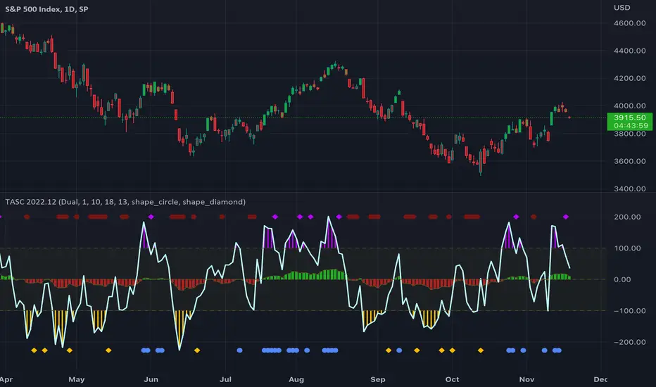
TASC 2022.12 Short-Term Continuation And Reversal Signals█ OVERVIEW
TASC's December 2022 edition Traders' Tips includes an article by Barbara Star titled "Short-Term Continuation And Reversal Signals". This is the code that implements the concepts presented in this publication.
█ CONCEPTS
The article takes two classic indicators, the Commodity Channel Index (CCI) and the Directional Movement Indicator (DMI), makes changes to the traditional ways of visualizing their readings, and uses them together to generate potential signals. The author first discusses the benefits of converting the DMI indicator to an oscillator format by subtracting the −DI from the +DI, which is then displayed as a histogram. Next, the author shows how the use of an on-chart visual framework (i.e., choosing the line style and color, coloring price bars, etc.) can help traders interpret the signals produced the considered pair of indicators.
█ CALCULATIONS
The article offers the following signals based on the readings of the DMI and CCI pair, suitable for several types of trades:
• Short-term trend change signals:
A DMI oscillator above zero indicates that prices are in an uptrend. A DMI oscillator below the zero line and falling means that selling pressure is dominating and price is trending down. The sign of the DMI oscillator is indicated by the color of the price bars (which correlates with the color of the DMI histogram). Namely, green, red and grey price bars correspond to the DMI oscillator above, below and equal to zero . Colored price bars and the DMI oscillator make it easy for trend traders to recognize changes in short-term trends.
• Trend continuation signals:
Blue circles appear near the bottom of the oscillator chart border when the DMI is above the zero line and the price is above its simple moving average in an uptrend . Dark red circles appear near the top of the chart in a downtrend when the DMI oscillator is below its zero line and below the 18-period moving average. Trend continuation signals are useful for those looking to add to existing positions, as well as for traders waiting for a pullback after a trend has started.
• Reversal signals:
The CCI signals a reversal to the downside when it breaks out of its +100 and then returns at some point, crossing below the +100 level. This is indicated by a magenta-colored diamond shape near the top the chart. The CCI signals a reversal to the upside when it moves below its −100 level and then at some point comes back to cross above the −100 level. This is indicated by a yellow diamond near the bottom of the chart. Reversal signals offer short-term rallies for countertrend traders as well as for swing traders looking for longer-term moves using the interplay between continuation and reversal signals.
Tasc
TASC 2022.11 Phasor Analysis█ OVERVIEW
TASC's November 2022 edition Traders' Tips includes an article by John Ehlers titled "Recurring Phase Of Cycle Analysis". This is the code that implements the phasor analysis indicator presented in this publication.
█ CONCEPTS
The article explores the use of phasor analysis to identify market trends.
An ordinary rotating phasor diagram is a two-dimensional vector, anchored to the origin, whose rotation rate corresponds to the cycle period in the price data stream. Similarly, Ehlers' phasor is a representation of angular phase rotation along the course of time. Its angle reflects the current phase of the cycle. Angles -180, -90, +90 and +180 degrees correspond to the beginning, valley, peak and end of the cycle, respectively.
If the observed cycle is very long, the market can be considered trending . In his article, John Ehlers defined trending behavior to occur when the derived instantaneous cycle period value is greater that 60 bars. The author also introduced guidelines for long and short entries in a trending state. Depending on the tuning of the indicator period input, a long entry position may occur when the phasor angle is around the approximate vicinity of −90 degrees, while a short entry position may occur when the phasor angle will be around the approximate vicinity of +90 degrees. Applying these definitive guidelines, the author proposed a state variable that is indicated by +1 for a trending long position, 0 for cycling, and −1 for a trending short position (or out).
The phasor angle, the cycle period, and the state variable are made available with three selectable display modes provided for this TradingView indicator.
█ CALCULATIONS
The calculations are carried out as follows.
First, the price data stream is correlated with cosine and sine of a fixed cycle period. This produces two new data streams that correspond to the projections of the frequency domain phasor diagram to the horizontal (so-called real ) and vertical (so-called imaginary ) axis respectively. The wavelength of the cycle period input should be set for the midrange vicinities of the phasor to coincide with the peaks and valleys of the charted price data.
Secondly, the phase angle of the phasor is easily computed as the arctangent of the ratio of the imaginary component to the real component. The difference between the current phasor values and its last is then employed to calculate a derived instantaneous period and market state. This computation is then repeated successively for each individual bar over the entire duration of the data set.

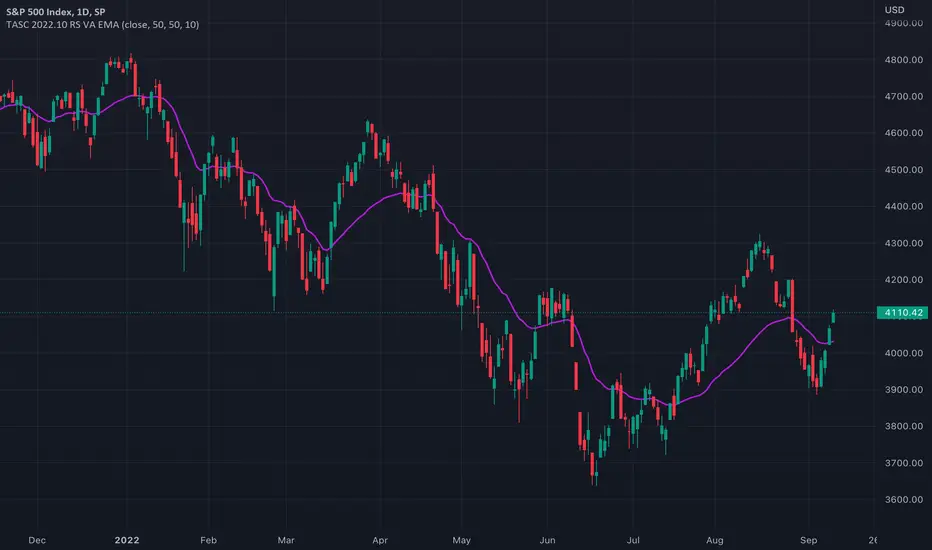
TASC 2022.10 RS VA EMA█ OVERVIEW
TASC's October 2022 edition Traders' Tips includes the second part of the "Relative Strength Moving Averages" article series authored by Vitali Apirine. This is the code that implements the Relative Strength Volume-Adjusted Exponential Moving Average (RS VA EMA) presented in this publication.
█ CONCEPTS
In his article series, the author argues that the relative strength of price, volume, and volatility can potentially be used to filter price movements and define turning points. In particular, the RS VA EMA indicator is designed to account for the relative strength of volume. Like the traditional exponential moving average (EMA) , it is a lagging trend-following indicator. The difference is that it responds more quickly.
In a trading strategy, RS VA EMA is suggested to be used in combination with EMA of the same length to determine the overall trend or in combination with RS VA EMA of a different length to identify turning points and filter price movements.
█ CALCULATIONS
The calculation of RS VA EMA is based on the concept of volume strength (VS). By definition, VS measures the difference between "positive" and "negative" volume flow. Volume is indicated as "positive" when the close is higher than the previous close and "negative" when the close is below the previous close.
The following steps are used in the calculation process:
• Calculate the volume strength (VS) of a given length.
• Multiply VS by a predefined multiplier and calculate the EMA of the resulting time series.
The values of 10,10,10 are the typical input settings for RS VA EMA, where the first parameter is the length of the moving average, the second is the length of VS, and the third is the volume strength multiplier.
TASC 2022.09 LRAdj EMA█ OVERVIEW
TASC's September 2022 edition of Traders' Tips includes an article by Vitali Apirine titled "The Linear Regression-Adjusted Exponential Moving Average". This script implements the titular indicator presented in this article.
█ CONCEPT
The Linear Regression-Adjusted Exponential Moving Average (LRAdj EMA) is a new tool that combines a linear regression indicator with exponential moving averages . First, the indicator accounts for the linear regression deviation, that is, the distance between the price and the linear regression indicator. Subsequently, an exponential moving average (EMA) smooths the price data and and provides an indication of the current direction.
As part of a trading system, LRAdj EMA can be used in conjunction with an exponential moving average of the same length to identify the overall trend. Alternatively, using LRAdj EMAs of different lengths together can help identify turning points.
█ CALCULATION
The script uses the following input parameters:
EMA Length
LR Lookback Period
Multiplier
The calculation of LRAdj EMA is carried out as follows:
Current LRAdj EMA = Prior LRAdj EMA + MLTP × (1+ LRAdj × Multiplier ) × ( Price − Prior LRAdj EMA ),
where MLTP is a weighting multiplier defined as MLTP = 2 ⁄ ( EMA Length + 1), and LRAdj is the linear regression adjustment (LRAdj) multiplier:
LRAdj = (Abs( Current LR Dist )−Abs( Minimum LR Dist )) ⁄ (Abs( Maximum LR Dist )−Abs( Minimum LR Dist ))
When calculating the LRAdj multiplier, the absolute values of the following quantities are used:
Current LR Dist is the distance between the current close and the linear regression indicator with a length determined by the LR Lookback Period parameter,
Minimum LR Dist is the minimum distance between the close and the linear regression indicator for the LR lookback period ,
Maximum LR Dist is the maximum distance between the close and the linear regression indicator for the LR lookback period .

TASC 2022.07 Pairs Rotation With Ehlers Loops█ OVERVIEW
TASC's July 2022 edition of Traders' Tips includes an article by John Ehlers titled "Pairs Rotation With Ehlers Loops". This is the code that implements the Ehlers Loops applied to pairs rotation trading.
█ CONCEPTS
John Ehlers developed Ehlers loops as a tool to visualize the performance of one data stream versus another. Initially, he used this tool to chart price versus volume. However, Ehlers loops proved to be suitable for determining the timing of the pairs rotation strategy . This strategy works by having a long position in only one of two securities, depending on which one is considered stronger at a given time.
When the prices of two securities (filtered and scaled with a standard deviation for consistent presentation) are plotted against each other, the curvature and direction of rotation on the chart can help guide decisions on long positions. For example, when plotting a stock versus a referenced symbol, a vertical upward movement while rotating clockwise is a sign of going long the stock. Similarly, a horizontal movement to the right while rotating counterclockwise is the sign to go long the reference. A higher probability of a reversal is expected when the price moves more than one or two standard deviations.
█ CALCULATIONS
The script uses the following steps to calculate the Ehlers Loops:
The price data of both securities in the pair are individually filtered using identical high-pass and SuperSmoother filters. This results in two band-limited data streams, having a nominally zero mean. The input parameters Low-Pass Period and High-Pass Period control the filter bandwidth and thus can modify the shape of the Ehlers Loops.
Subsequently, the filtered data streams are scaled in terms of standard deviation by dividing each of them by their root-mean-square (RMS) values. These data streams are plotted as zero-mean oscillators.
Finally, the scaled data streams are displayed one against another for the selected time interval (defined by the input parameter Loop Segments ). In the resulting scatterplot, the thicker line corresponds to the later data points. The fluctuations of the filtered price data of the chart symbol are plotted along the y -axis, and the price changes of the referenced symbol are shown along the x -axis.

TASC 2022.6 Ehlers' Loops - SectorsInspired by the latest TASC article, the crocker graph is expanded to show 5 tickers.
for commodity also draws a side box with current tickers candles so it can be used as standalone.

TASC 2022.06 Ehlers Loops█ OVERVIEW
TASC's June 2022 edition Traders' Tips includes an article by John Ehlers titled "Ehlers Loops. Part 1". This is the code implementing the price-volume Ehlers Loops he introduced in the publication.
█ CONCEPTS
John Ehlers developed Ehlers loops as a tool to visualize the performance of one data stream versus another, both filtered and scaled. In this article, the author applies his concept to exploit and/or dispel the dogmatic principles of reliable price-volume relationships.
The script offers two different ways to visualize Ehlers Loops:
Oscillators (default option)
In this implementation, filtered and scaled volume is plotted along with filtered and scaled price as zero-mean oscillators. Observation of the relative direction of volume and price oscillators can be discretionarily used to interpret and predict market conditions. For example, it is generally assumed that an increase in volume and an increase in price define a bullish condition. Similarly, decreasing volume and increasing price are generally considered bearish. A decrease in volume and a decrease in price is considered a bullish condition. The increase in volume and decrease in price is often thought to be bearish.
Scatterplot
This Crocker-style visualization displays filtered and scaled price against filtered and scaled volume for the selected timespan. Fluctuations in volume are plotted along the x -axis, while price changes along the y -axis. This way of visualizing the Ehlers Loop allows you to analyze the curvature and directional path of the price in relation to volume, offering a different comparative perspective. The boundaries of the price and volume scale on the Ehlers Loop Crocker-chart are presented in standard deviations. Deviations can be used to predict possible future price or volume fluctuations. The expected probability of potential reversals is 68%, 95% and 99.7% at one, two and three standard deviations, respectively.
█ CALCULATIONS
The following steps are used to build an Ehlers Loop:
• Both price and volume are filtered to be band-limited signals. This is done by applying the high-pass Butterworth filter in combination with the low-pass SuperSmooth filter.
The cutoff wavelengths of the high-pass and low-pass filters are defined by the input parameters HPPeriod and LPPeriod , respectively.
These values change the appearance of the Ehlers Loops and can be customized to your trading style.
• The filtered price and volume time series are then scaled in terms of standard deviation by dividing each by their root-mean-square values.
• The resultant price and volume data are plotted as zero-mean oscillators or as a scatterplot.

TASC 2022.05 Relative Strength Exponential Moving Average█ OVERVIEW
TASC's May 2022 edition Traders' Tips includes the "Relative Strength Moving Averages" article authored by Vitali Apirine. This is the code implementing the Relative Strength Exponential Moving Average (RS EMA) indicator introduced in this publication.
█ CONCEPTS
RS EMA is an adaptive trend-following indicator with reduced lag characteristics. By design, this was made possible by harnessing the relative strength of price. It operates in a similar fashion to a traditional EMA, but it has an improved response to price fluctuations. In a trading strategy, RS EMA can be used in conjunction with an EMA of the same length to identify the overall trend (see the preview chart). Alternatively, RS EMAs with different lengths can define turning points and filter price movements.
RS EMA is an adaptive trend-following indicator with reduced lag characteristics. By design, this was made possible by harnessing the relative strength of price. It operates in a similar fashion to a traditional EMA, but it has an improved response to price fluctuations.
█ CALCULATIONS
The following steps are used in the calculation process:
• Calculate the relative strength (RS) of a given length.
• Multiply RS by a chosen coefficient (multiplier) to adapt the EMA filtering the original time series. Calculate the EMA of the resulting time series.
The author recommends RS EMA(10,10,10) as typical settings, where the first parameter is the EMA length, the second parameter is the RS length, and the third parameter is the RS multiplier. Other values may be substituted depending on your trading style and goals.
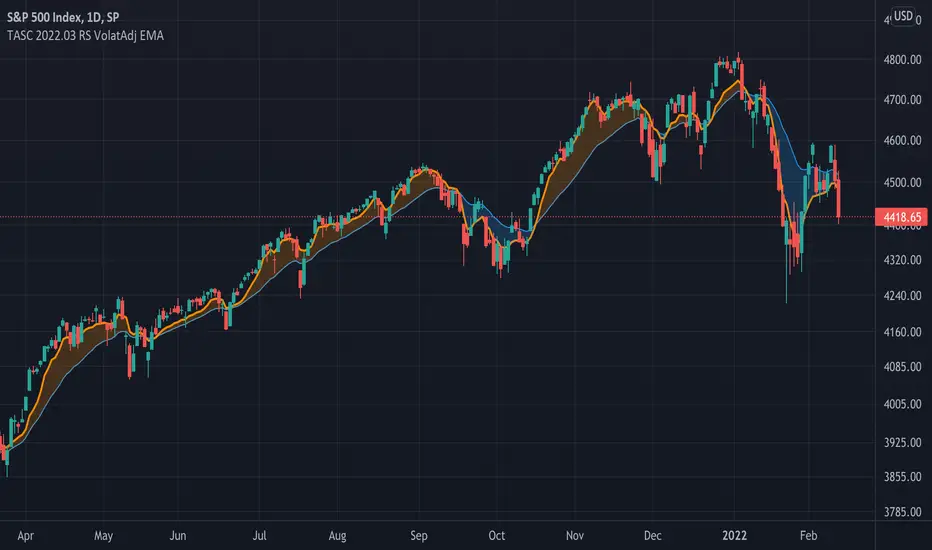
TASC 2022.03 Relative Strength Volatility-Adjusted EMA█ OVERVIEW
TASC's March 2022 edition of Traders' Tips includes the "Relative Strength Moving Averages - Part 3: The Relative Strength Volatility-Adjusted Exponential Moving Average" article authored by Vitali Apirine. This is the code that implements the "RS VolatAdj EMA" from the article.
█ CONCEPTS
In a three-part article series, Vitaly Apirine examines ways to filter price movements and define turning points by applying the Relative Strength concept to exponential moving averages . The resulting indicator is more responsive and is intended to account for the relative strength of volatility .
█ CALCULATIONS
The calculation process uses the following steps:
Select an appropriate volatility index (in our case it is VIX ).
Calculate up day volatility (UV) smoothed by a 10-day EMA.
Calculate down day volatility (DV) smoothed by a 10-day EMA.
Take the absolute value of the difference between UV and DV and divide by the sum of UV and DV. This is the Volatility Strength we need.
Calculate a MLTP constant - the weighting multiplier for an exponential moving average.
Combine Volatility Strength and MLTP to create an exponential moving average on current price data.
Join TradingView!
TASC 2022.02 Ehlers' Elegant Oscillator█ OVERVIEW
TASC's February 2022 edition of Traders' Tips includes the "Inverse Fisher Transform Redux — An Elegant Oscillator" article authored by John Ehlers. This is the code implementing the "Elegant Oscillator" from the article.
█ CONCEPTS
By applying the inverse Fisher transform to a waveform with a nominal Gaussian probability distribution using root mean square ( RMS ) scaling and smoothing the result, John Ehlers creates an oscillator that swings between -1 and 1.
█ CALCULATIONS
The calculation process uses the following steps:
• Compute the 2-bar difference of closing prices.
• Calculate the root mean square (RMS) of the differences.
• Scale the differences using the computed RMS.
• Apply the inverse Fisher transform to the scaled values.
• Smooth the transformed data with the SuperSmoother filter.
Join TradingView!

TASC 2022.01 Improved RSI w/Hann█ OVERVIEW
TASC's January 2022 edition Traders' Tips includes the "(Yet Another Improved) RSI Enhanced With Hann Windowing" article authored by John Ehlers. Once again John Ehlers revolutionizes the RSI indicator. This is TradingView's Pine Script code for the indicator.
█ CONCEPTS
By employing a Hann windowed finite impulse response filter ( FIR ), John Ehlers has enhanced the "Relative Strength Indicator" ( RSI ) to provide an improved oscillator with exceptional smoothness.
█ NOTES
Calculations
The method of calculations using "closes up" and "closes down" from Welles Wilder's RSI described in his 1978 book is still inherent to Ehlers enhanced formula. However, a finite impulse response (FIR) Hann windowing technique is employed following the closes up/down calculations instead of the original Wilder infinite impulse response averaging filter. The resulting oscillator waveform is confined between +/-1.0 with a 0.0 centerline regardless of chart interval, as opposed to Wilder's original formulation, which was confined between 0 and 100 with a centerline of 50. On any given trading timeframe, the value of Ehlers' enhanced RSI found above the centerline typically represents an overvalued region, while undervalued regions are typically found below the centerline.
Background
The original RSI indicator was designed by J. Welles Wilder and presented in his "New Concepts in Technical Trading Systems" book published in 1978.
Join TradingView!

TASC 2021.12 Directional Movement w/Hann█ OVERVIEW
Presented here is code for the "Directional Movement w/Hann" indicator originally conceived by John Ehlers. The code is also published in the December 2021 issue of Trader's Tips by Technical Analysis of Stocks & Commodities (TASC) magazine.
Ehlers continues here his exploration of the application of Hann windowing to conventional trading indicators.
█ FEATURES
The rolling length can be modified in the script's inputs, as well as the width of the line.
█ NOTES
Calculations
The calculation starts with the classic definition of PlusDM and MinusDM. These directional movements are summed in an exponential moving average (EMA). Then, this EMA is further smoothed in a finite impulse response (FIR) filter using Hann window coefficients over the calculation period.
Background
The DMI and ADX indicators were designed by J. Welles Wilder and presented in his "New Concepts in Technical Trading Systems" book published in 1978.
Join TradingView!

TASC 2021.11 MADH Moving Average Difference, Hann█ OVERVIEW
Presented here is code for the "Moving Average Difference, Hann" indicator originally conceived by John Ehlers. The code is also published in the November 2021 issue of Trader's Tips by Technical Analysis of Stocks & Commodities (TASC) magazine.
█ CONCEPTS
By employing a Hann windowed finite impulse response filter (FIR), John Ehlers has enhanced the Moving Average Difference (MAD) to provide an oscillator with exceptional smoothness.
Of notable mention, the wave form of MADH resembles Ehlers' "Reverse EMA" Indicator, formerly revealed in the September 2017 issue of TASC. Many variations of the "Reverse EMA" were published in TradingView's Public Library.
█ FEATURES
Three values in the script's "Settings/Inputs" provide control over the oscillators behavior:
• The price source
• A "Short Length" with a default of 8, to manage the lower band edge of the oscillator
• The "Dominant Cycle", originally set at 27, which appears to be a placeholder for an adaptive control mechanism
Two coloring options are provided for the line's fill:
• "ZeroCross", the default, uses the line's position above/below the zero level. This is the mode used in the top version of MADH on this chart.
• "Momentum" uses the line's up/down state, as shown in the bottom version of the indicator on the chart.
█ NOTES
Calculations
The source price is used in two independent Hann windowed FIR filters having two different periods (lengths) of historical observation for calculation, one being a "Short Length" and the other termed "Dominant Cycle". These are then passed to a "rate of change" calculation and then returned by the reusable function. The secret sauce is that a "windowed Hann FIR filter" is superior tp a generic SMA filter, and that ultimately reveals Ehlers' clever enhancement. We'll have to wait and see what ingenuities Ehlers has next to unleash. Stay tuned...
The `madh()` function code was optimized for computational efficiency in Pine, differing visibly from Ehlers' original formula, but yielding the same results as Ehlers' version.
Background
This indicator has a sibling indicator discussed in the "The MAD Indicator, Enhanced" article by Ehlers. MADH is an evolutionary update from the prior MAD indicator code published in the October 2021 issue of TASC.
Sibling Indicators
• Moving Average Difference (MAD)
• Cycle/Trend Analytics
Related Information
• Cycle/Trend Analytics And The MAD Indicator
• The Reverse EMA Indicator
• Hann Window
• ROC
Join TradingView!

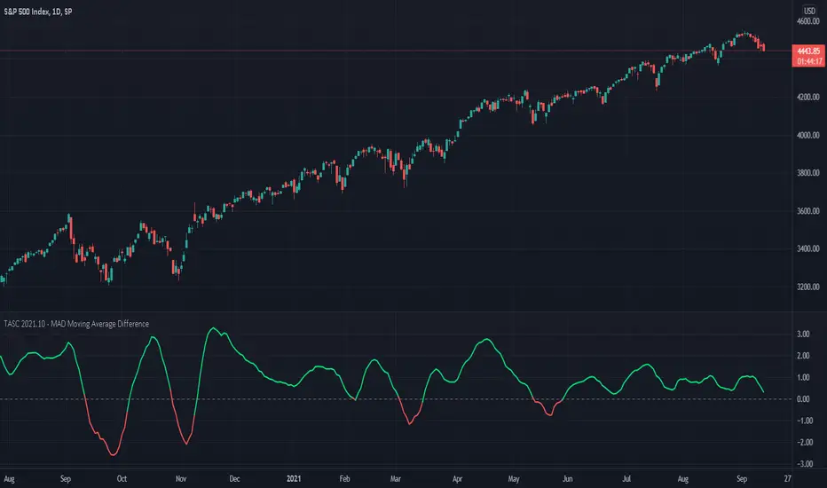
TASC 2021.10 - MAD Moving Average DifferencePresented here is code for the "Moving Average Difference" indicator originally conceived by John Ehlers, also referred to as MAD. This is one of TradingView's first code releases published in the October 2021 issue of Trader's Tips by Technical Analysis of Stocks & Commodities (TASC) magazine.
This indicator has a companion indicator that is discussed in the article entitled Cycle/Trend Analytics And The MAD Indicator , authored by John Ehlers. He's providing an innovative double dose of indicator code for the month of October 2021.
John Ehlers generally describes it as a "thinking man's" MACD . MAD has similar, yet distinct, intended operation. For those of you familiar with the MACD indicator operation, you will find MACD adjustments having defaults of 12 and 26, while MAD has comparable adjustments with defaults of 8 and 23. These are intended for adjustment, same as any other oscillator.
The MAD indicator can be basically described as two simple moving averages applied within a "rate of change" (ROC) calculation.
Further Related Information
• SMA
• ROC
Join TradingView!
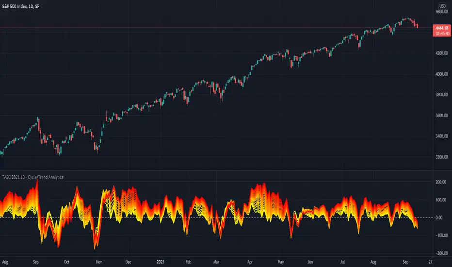
TASC 2021.10 - Cycle/Trend AnalyticsPresented here is code for the "Cycle/Trend Analytics" indicator originally conceived by John Ehlers. This is another one of TradingView's first code releases published in the October 2021 issue of Trader's Tips by Technical Analysis of Stocks & Commodities (TASC) magazine.
This indicator, referred to as "CTA" in later explanations, has a companion indicator that is discussed in the article entitled MAD Moving Average Difference , authored by John Ehlers. He's providing an innovative double dose of indicator code for the month of October 2021.
Modes of Operation
CTA has two modes defined as "trend" and "cycle". Ehlers' intention from what can be gathered from the article is to portray "the strength of the trend" in trend mode on real data. Cycle mode exhibits the response of the bank of calculations when a hypothetical sine wave is utilized as price. When cycle mode is chosen, two other lines will be displayed that are not shown in trend mode. A more detailed explanation of the indicator's technical functionality and intention can be found in the original Cycle/Trend Analytics And The MAD Indicator article, which requires a subscription.
Computational Functionality
The CTA indicator only has one adjustment in the indicator "Settings" for choice of modes. The default mode of operation is "trend". Trend mode applies raw price data to the bank of plots, while the cycle mode employs a sinusoidal oscillator set to a cycle period of 30 bars. These are passed to multiple SMAs, which are then subtracted from the original source data. The result is a fascinating display of plots embellished with vivid array of gradient color on real data or the hypothetical sine wave.
Related Information
• SMA
• color.rgb()
Join TradingView
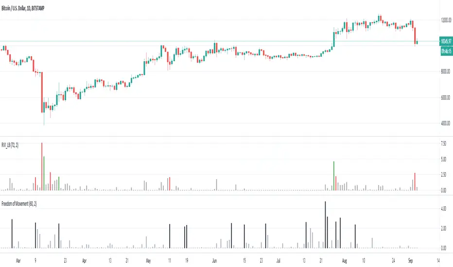
Freedom of MovementFreedom of Movement Indicator
---------------------------------------------------------
In “Evidence-Based Support & Resistance” article, author Melvin Dickover introduces two new indicators to help traders note support and resistance areas by identifying supply and demand pools. Here you can find the support-resistance technical indicator called "Freedom of Movement".
The indicator takes into account price-volume behavior in order to detect points where movement of price is suddenly restricted, the possible supply and demand pools. These points are also marked by Defended Price Lines (DPLs).
DPLs are horizontal lines that run across the chart at levels defined by following conditions:
* Overlapping bars: If the indicator spike (i.e., indicator is above 2.0 or a custom value) corresponds to a price bar overlapping the previous one, the previous close can be used as the DPL value.
* Very large bars: If the indicator spike corresponds to a price bar of a large size, use its close price as the DPL value.
* Gapping bars: If the indicator spike corresponds to a price bar gapping from the previous bar, the DPL value will depend on the gap size. Small gaps can be ignored: the author suggests using the previous close as the DPL value. When the gap is big, the close of the latter bar is used instead.
* Clustering spikes: If the indicator spikes come in clusters, use the extreme close or open price of the bar corresponding to the last or next to last spike in cluster.
DPLs can be used as support and resistance levels. In order confirm and refine them, FoM (Freedom of Movement) is used along with the Relative Volume Indicator (RVI), which you can find here:
Clustering spikes provide the strongest DPLs while isolated spikes can be used to confirm and refine those provided by the RVI. Coincidence of spikes of the two indicator can be considered a sign of greater strength of the DPL.
More info:
S&C magazine, April 2014.
Reflex & Trendflex█ OVERVIEW
Reflex and Trendflex are zero-lag oscillators that decompose price into independent cycle and trend components using SuperSmoother filtering. These indicators isolate each component separately, providing clearer identification of cyclical reversals (Reflex) versus trending movements (Trendflex).
Based on Dr. John F. Ehlers' "Reflex: A New Zero-Lag Indicator" article (February 2020, TASC), both oscillators use normalized slope deviation analysis to minimize lag while maintaining signal clarity. The SuperSmoother filter removes high-frequency noise, then deviations from linear regression (Reflex) or current value (Trendflex) are measured and normalized by RMS for consistent amplitude across instruments and timeframes.
█ CONCEPTS
SuperSmoother Filter
Both oscillators begin with a two-pole Butterworth low-pass filter that smooths price data without the excessive lag of simple moving averages. The filter uses exponential decay coefficients and cosine modulation based on the cutoff period, providing aggressive smoothing while preserving signal timing.
Reflex: Cycle Component
Reflex isolates cyclical price behavior by measuring deviation from a linear regression line fitted through the SuperSmoother output. For each bar, the filter calculates a linear slope over the lookback period, then sums how much the smoothed price deviates from this trendline. These deviations represent pure cyclical movement - price oscillations around the dominant trend. The result is normalized by RMS (root mean square) to produce consistent amplitude regardless of volatility or timeframe.
Trendflex: Trend Component
Trendflex extracts trending behavior by measuring cumulative deviation from the current SuperSmoother value. Instead of comparing to a regression line, it simply sums the differences between the current smoothed value and all past values in the period. This captures sustained directional movement rather than oscillations. Like Reflex, normalization by RMS ensures comparable readings across different instruments.
RMS Normalization
Both oscillators normalize their raw deviation measurements using an exponentially weighted RMS calculation: `rms = 0.04 * deviation² + 0.96 * rms `. This adaptive normalization ensures the oscillator amplitude remains stable as volatility changes, making threshold levels meaningful across different market conditions.
█ INTERPRETATION
Reflex (Cycle Component)
Oscillates around zero representing cyclical price behavior isolated from trend:
• Above zero : Price is in upward phase of cycle
• Below zero : Price is in downward phase of cycle
• Zero crossings : Potential cycle reversal points
• Extremes : Indicate stretched cyclical condition, often precede mean reversion
Best used for identifying cyclical turning points in ranging or oscillating markets. More sensitive to reversals than Trendflex.
Trendflex (Trend Component)
Oscillates around zero representing trending behavior isolated from cycles:
• Above zero : Sustained upward trend
• Below zero : Sustained downward trend
• Zero crossings : Trend direction changes
• Magnitude : Strength of trend (larger absolute values = stronger trend)
Best used for confirming trend direction and identifying trend exhaustion. Less noisy than Reflex due to focus on directional movement rather than oscillations.
Combined Analysis
Using both oscillators together provides powerful signal confirmation:
• Both positive: Strong uptrend with positive cycle phase (high probability long setup)
• Both negative: Strong downtrend with negative cycle phase (high probability short setup)
• Divergent signals: Conflicting cycle and trend (choppy conditions, reduce position size)
• Reflex reversal with Trendflex agreement: Cyclical turn within established trend (entry/exit timing)
Dynamic Thresholds
Threshold bands identify statistically significant oscillator readings that warrant attention:
• Breach above +threshold : Strong bullish cycle (Reflex) or trend (Trendflex) behavior - potential overbought condition
• Breach below -threshold : Strong bearish cycle or trend behavior - potential oversold condition
• Return inside thresholds : Signal strength normalizing, potential reversal or consolidation ahead
• Threshold compression : During low volatility, thresholds narrow (especially with StdDev mode), making breaches more frequent
• Threshold expansion : During high volatility, thresholds widen, filtering out minor oscillations
Combine threshold breaches with zero-line position for stronger signals:
• Threshold breach + zero-line cross = high-conviction signal
• Threshold breach without zero-line support = monitor for confirmation
Alert Conditions
Six built-in alerts trigger on bar close (no repainting):
• Above +Threshold : Oscillator crossed above positive threshold (strong bullish behavior)
• Below -Threshold : Oscillator crossed below negative threshold (strong bearish behavior)
• Reflex Above Zero : Reflex crossed above zero (bullish cycle phase)
• Reflex Below Zero : Reflex crossed below zero (bearish cycle phase)
• Trendflex Above Zero : Trendflex crossed above zero (bullish trend shift)
• Trendflex Below Zero : Trendflex crossed below zero (bearish trend shift)
█ SETTINGS & PARAMETER TUNING
Oscillator Settings
• Source : Price series to decompose
• Reflex Period (5-50): SuperSmoother period for cycle component. Lower values increase responsiveness to cyclical turns but add noise. Default 20.
• Trendflex Period (5-50): SuperSmoother period for trend component. Lower values respond faster to trend changes. Default 20.
Display Settings
• Reflex/Trendflex Display : Toggle visibility and customize colors for each oscillator independently
• Zero Line : Reference line showing neutral oscillator position
Dynamic Thresholds
Optional significance bands that identify when oscillator readings indicate strong cyclical or trending behavior:
• Threshold Mode : Choose calculation method based on market characteristics
- MAD (Median Absolute Deviation) : Outlier-resistant, best for markets with occasional spikes (default)
- Standard Deviation : Volatility-sensitive, adapts quickly to regime changes
- Percentile Rank : Fixed probability bands (e.g., 90% = only 10% of values exceed threshold)
• Apply To : Select which oscillator (Reflex or Trendflex) to calculate thresholds for
• Period (2-200): Lookback window for threshold calculation. Default 50.
• Multiplier (k) : Scaling factor for MAD/StdDev modes. Higher values = fewer threshold breaches (default 1.5)
• Percentile (%) : For Percentile mode only. Higher percentile = more selective threshold (default 90%)
Parameter Interactions
• Shorter periods make both oscillators more sensitive but noisier
• Reflex typically more volatile than Trendflex at same period settings
• For ranging markets: shorter Reflex period (10-15) captures swings better
• For trending markets: shorter Trendflex period (10-15) follows trend shifts faster
█ LIMITATIONS
Inherent Characteristics
• Near-zero lag, not zero-lag : Despite the name, some lag remains from SuperSmoother filtering
• Normalization artifacts : RMS normalization can produce unusual readings during volatility regime changes
• Period dependency : Oscillator characteristics change significantly with different period settings - no "correct" universal parameter
Market Conditions to Avoid
• Very low volatility : Normalization amplifies noise in quiet markets, producing false signals
• Sudden gaps : SuperSmoother assumes continuous data; large gaps disrupt filter continuity requiring bars to stabilize
• Micro timeframes : Sub-minute charts contain microstructure noise that overwhelms signal quality
Parameter Selection Pitfalls
• Matching periods to dominant cycle : If period doesn't align with actual market cycle period, signals degrade
• Threshold over-tuning : Optimizing threshold parameters for past data often fails forward - use conservative defaults
• Ignoring component differences : Reflex and Trendflex measure different aspects - don't expect identical behavior
█ NOTES
Credits
These indicators are based on Dr. John F. Ehlers' "Reflex: A New Zero-Lag Indicator" published in the February 2020 issue of Technical Analysis of Stocks & Commodities (TASC) magazine. The article introduces a novel approach to isolating cycle and trend components using SuperSmoother filtering combined with normalized deviation analysis.
For those interested in the underlying mathematics and DSP concepts:
• Ehlers, J.F. (February 2020). "Reflex: A New Zero-Lag Indicator" - Technical Analysis of Stocks & Commodities magazine
• Ehlers, J.F. (2001). Rocket Science for Traders: Digital Signal Processing Applications . John Wiley & Sons
• Various TASC articles by John Ehlers on SuperSmoother filters and oscillator design
by ♚@e2e4

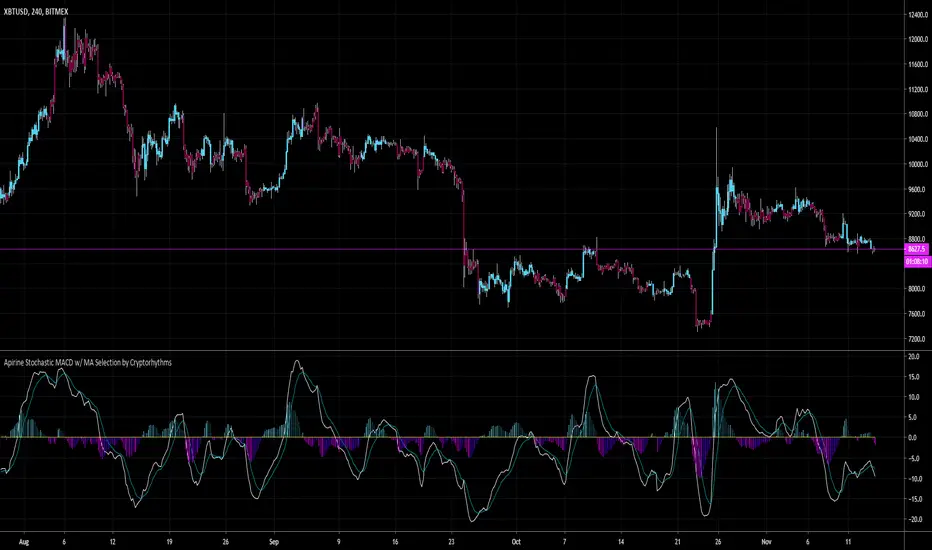
Apirine Stochastic MACD w/ MA Selection by Cryptorhythms📊 Apirine Stochastic MACD w/ MA Selection by Cryptorhythms
Intro
Had to re-release due to moderation.
This happens to be my first open source indicator, hope you all enjoy it!
Description
This indicated is ported from November 2019 issue of TASC. “The Stochastic MACD Oscillator” in this issue, author Vitali Apirine introduces a new indicator created by combining the stochastic oscillator and the MACD . He describes the new indicator as a momentum oscillator and explains that it allows the trader to define overbought and oversold levels similar to the classic stochastic but based on the MACD .
Options
-You can enable bar coloration for trade state (signal conditions setup in the "long" and "short" variables).
-You can choose histogram or columns for the convergence/divergence display.
-You can turn on/off and adjust the overbought / oversold zones.
-You can choose what type of moving average to use in the calculation from a small selection of options. This gives you more flexibility to adapt the indicator to your needs.
👍 We hope you enjoyed this indicator and find it useful! We post free crypto analysis, strategies and indicators regularly. This is our 70th script on Tradingview!
🤐Check my Signature for other information
Fourier series Model Of The Market█ OVERVIEW
The Fourier Series Model of the Market (FSMM) decomposes price action into harmonic components using bandpass filtering, then reconstructs a composite wave weighted by rolling energy ratios. This approach isolates cyclical market behavior at multiple frequencies, emphasizing dominant cycles for cleaner signal generation. The energy-adaptive weighting is the key differentiator from simple harmonic summation: cycles that dominate current price action contribute more to the output.
Based on Fourier analysis principles applied to financial markets, the indicator extracts harmonics (fundamental, 2nd, 3rd, etc.) using second-order IIR bandpass filters, then weights each harmonic's contribution by its relative energy compared to adjacent harmonics. This energy-adaptive weighting naturally emphasizes the cycles that are most prominent in current market conditions.
█ CONCEPTS
Fourier Decomposition
Fourier analysis represents any periodic signal as a sum of sine waves at different frequencies. In market analysis, price action can be decomposed into a fundamental cycle (the base period) plus harmonics at integer multiples of that frequency (period/2, period/3, etc.). Each harmonic captures oscillations at a specific frequency band, and their sum reconstructs the original cyclical behavior.
Bandpass Filtering
Each harmonic is extracted using a second-order IIR (Infinite Impulse Response) bandpass filter tuned to that harmonic's frequency. The filter isolates price activity within a narrow frequency range while rejecting both higher-frequency noise and lower-frequency trend drift. Before filtering, the source is debiased via 2-bar momentum to remove DC offset, ensuring each bandpass operates around true zero.
Energy-Weighted Reconstruction
Rather than simply summing all harmonics equally, FSMM weights each harmonic by its rolling energy relative to the previous harmonic. The energy score combines the current harmonic value with its rate of change, so it reflects both amplitude and momentum. Higher harmonics that hold comparatively more energy therefore contribute more to the composite wave, while weaker harmonics fade out. This adaptive weighting allows the model to respond to changing market cyclicality.
Quadrature Component (Rate of Change)
The rate of change output represents the 90°-phase-shifted (quadrature) component of the wave. When the wave is at zero and rising, the rate of change is at maximum positive. This provides complementary information about cycle phase and can be used for timing entries relative to cycle position.
█ INTERPRETATION
Wave Output
The composite wave oscillates around zero, representing the sum of all extracted harmonic components weighted by energy:
• Above zero : Net bullish cyclical momentum across harmonics
• Below zero : Net bearish cyclical momentum across harmonics
• Zero crossings : Cycle phase transitions - potential reversal points
• Wave amplitude : Strength of cyclical behavior; larger swings indicate cleaner cycles
Rate of Change
The quadrature component (90° phase-shifted) provides cycle phase information:
• Maximum rate of change : Wave is near zero and accelerating - early cycle phase
• Zero rate of change : Wave is at peak or trough - cycle extremes
• Rate/Wave divergence : When wave makes new highs/lows but rate of change does not confirm (lower momentum), suggests cycle exhaustion or impending phase shift
Combined Analysis
• Wave crossing above zero with positive rate of change: Strong bullish cycle initiation
• Wave crossing below zero with negative rate of change: Strong bearish cycle initiation
• Wave at extreme with rate of change reversing: Potential cycle peak/trough
Threshold Bands
When enabled, threshold bands define statistically significant wave deviations:
• Breach above +threshold : Unusually strong bullish cyclical behavior
• Breach below -threshold : Unusually strong bearish cyclical behavior
• Return inside thresholds : Normalizing behavior, potential mean reversion ahead
Alert Conditions
Four built-in alerts trigger on bar close (no repainting):
• Above +Threshold : Strong bullish cycle behavior
• Below -Threshold : Strong bearish cycle behavior
• Above Zero : Bullish cycle phase shift
• Below Zero : Bearish cycle phase shift
█ SETTINGS & PARAMETER TUNING
Fourier Series Model
• Source : Price series to decompose into harmonic components.
• Period (6-100): Base period for the fundamental harmonic. Higher harmonics divide this period (harmonic 2 = period/2, harmonic 3 = period/3). Match to the dominant market cycle for best results. Default 20.
• Bandwidth (0.05-0.5): Bandpass filter selectivity. Lower values create narrower passbands that isolate harmonics more precisely but may miss slightly off-frequency cycles. Higher values capture broader ranges but reduce harmonic separation. Default 0.1 balances precision and robustness.
• Harmonics (1-20): Number of harmonic components to extract. More harmonics capture finer cyclical detail but increase computation. For most applications, 3-5 harmonics suffice. The fundamental alone (1 harmonic) functions as a simple bandpass filter.
Display Settings
• Wave Outputs : Toggle visibility and color of the composite Fourier wave.
• Rate of Change : Toggle visibility and color of the quadrature component (90° phase-shifted wave).
• Zero Line : Reference line for oscillator neutrality.
Diagnostics - Dynamic Thresholds
Optional significance bands that identify when wave readings indicate strong cyclical behavior:
• Dynamic Threshold : Toggle threshold bands and set colors.
• Threshold Mode : Select calculation method:
- MAD (Median Absolute Deviation) : Robust, outlier-resistant measure using k * MAD where MAD ≈ 0.6745 * stdev.
- Standard Deviation : Volatility-sensitive, calculated as k * stdev of wave over the lookback period.
- Percentile Rank : Fixed probability bands using percentile of |wave| (90% means only 10% of values exceed threshold).
• Period (2-200): Lookback for threshold calculations. Default 50.
• Multiplier (k) : Scaling for MAD/Standard Deviation modes. Default 1.5.
• Percentile (%) (0-100): For Percentile Rank mode only. Default 90%.
Parameter Interactions
• Shorter periods respond faster to cycle changes but may capture noise.
• Lower bandwidth + more harmonics = more precise decomposition but requires accurate period setting.
• Higher bandwidth is more forgiving of period mismatches.
• For strongly trending markets, restrict harmonics to 1-2 so the model tracks the dominant cycle with fewer higher-frequency components.
• For ranging/oscillating markets, more harmonics (4-6) capture complex cycles.
█ LIMITATIONS
Inherent Characteristics
• Period dependency : Effectiveness depends on correctly matching the Period parameter to actual market cycles. Use cycle measurement tools (autocorrelation, FFT, dominant cycle indicators) to identify appropriate periods.
• Stationarity assumption : The indicator assumes cycle frequencies remain relatively stable within the lookback window. Rapidly shifting dominant cycles (regime transitions) may produce inconsistent results until the buffer adapts.
• Filter lag : Despite bandpass design, some lag remains inherent to causal filtering. Higher harmonics have less lag but more noise sensitivity.
• Energy weighting artifacts : During regime changes when harmonic energy ratios shift rapidly, weighting may produce transient anomalies.
Market Conditions to Avoid
• Strong trending markets : Pure trends with no cyclicality produce weak, meandering signals. The indicator assumes cyclical market behavior.
• News events/gaps : Large discontinuities disrupt filter continuity. Requires 1-2 full periods to stabilize.
• Period mismatch : If the Period parameter doesn't match actual market cycles, harmonic extraction produces noise rather than signal.
Parameter Selection Pitfalls
• Too many harmonics : Beyond 5-6 harmonics, additional components often capture noise rather than meaningful cycles.
• Bandwidth too narrow : Very low bandwidth (< 0.05) requires extremely precise period matching; slight mismatches cause signal loss.
• Over-optimization : Perfect historical parameter fits typically fail forward. Use robust defaults across multiple instruments.
█ NOTES
Credits
This indicator applies Fourier analysis principles to financial market data, building on the extensive work of Dr. John F. Ehlers in applying digital signal processing to trading. The bandpass filter implementation and harmonic decomposition approach draw from DSP fundamentals as presented in Ehlers' publications.
For those interested in the underlying mathematics and DSP concepts:
• Ehlers, J.F. (2001). Rocket Science for Traders: Digital Signal Processing Applications . John Wiley & Sons.
• Ehlers, J.F. (2013). Cycle Analytics for Traders . John Wiley & Sons.
• Various TASC articles by John Ehlers on bandpass filters, cycle analysis, and harmonic decomposition.
by ♚@e2e4

Voss Predictive Filter█ OVERVIEW
The Voss Predictive Filter (VPF) is a negative group delay (NGD) filter that anticipates cyclical price movement through phase compensation. The VPF isolates band-limited cyclical components via a bandpass filter, then applies negative group delay to shift the signal's phase forward, causing the output to lead the input by a fraction of the cycle period.
Based on Dr. John F. Ehlers' "Voss Predictive Filter" article in Technical Analysis of Stocks & Commodities (TASC) magazine, the VPF displays a predictive oscillator with optional dynamic threshold bands for identifying significant cycle behavior. The indicator is timeframe-agnostic - the mathematics work identically from tick charts to monthly bars, though shorter timeframes require more careful parameter selection due to noise.
█ CONCEPTS
Bandpass Filtering
A bandpass filter isolates price activity within a specific frequency range, removing both high-frequency noise and low-frequency trend drift. The VPF uses a second-order IIR (Infinite Impulse Response) bandpass filter characterized by the center frequency (the Bandpass Period input) and bandwidth. The center frequency determines which cycle period the filter emphasizes, while bandwidth controls the damping coefficient - how tightly the filter focuses around that frequency. Before filtering, the source is debiased via 2-bar momentum to remove DC offset, ensuring the filter operates around a true zero centerline.
Negative Group Delay Filtering
The predictive capability stems from negative group delay (NGD) - a filter characteristic where output appears to "lead" the input. Most causal filters introduce lag (positive group delay), but by combining the bandpass filter output with appropriately weighted past values, the VPF achieves negative group delay characteristics.
This is a universal NGD filter application for band-limited signals: the bandpass filter isolates the cyclical component of interest, then the NGD stage advances the phase within this limited frequency range to create an anticipatory output. This isn't statistical forecasting; it's phase compensation that shifts the signal's timing forward, causing peaks and troughs to appear before they occur in the bandpass output.
Negative Group Delay Stage
The NGD stage combines the current bandpass output with weighted historical values to produce an output that leads the input. By subtracting a weighted average of past deviations from a scaled version of the current filter value, the algorithm advances the signal's phase: peaks and zero-crossings in the voss output appear before the corresponding events in the bandpass filter.
The prediction order (`3 * Prediction Multiplier`) controls how many past values contribute to the phase advance. Higher orders provide smoother output but reduce the leading effect; lower orders maximize anticipation at the cost of stability.
█ INTERPRETATION
Zero-Line Crossovers
Crossings above zero suggest bullish momentum in the filtered cycle; below zero suggests bearish momentum. Crossings from near-zero regions are most reliable, as extreme excursions need time to return to equilibrium.
Threshold Bands
Threshold bands define "significant" deviation. Breaches indicate unusually strong behavior and can serve as:
• Trend confirmation when aligned with price direction
• Overbought/oversold warnings at extremes
• Trade entry filters (requiring threshold breach in the intended direction)
Threshold Mode affects sensitivity: MAD (outlier-resistant), Standard Deviation (volatility-sensitive), Percentile Rank (fixed probability bands).
Alert Conditions
Four built-in alerts trigger on bar close (no repainting): Above +Threshold (strong bullish cycle), Below -Threshold (strong bearish cycle), Above Zero (bullish phase shift), Below Zero (bearish phase shift).
█ SETTINGS & PARAMETER TUNING
Voss Predictive Filter
• Source : Price series to filter.
• Bandpass Period (1-100): Primary tuning parameter determining which cycle length the filter emphasizes. Short periods (8-15) are more responsive but noisier; medium periods (16-30) balance responsiveness and smoothness; long periods (31-100) focus on longer cycles with more smoothing.
• Bandwidth (0.01-0.45): Controls filter selectivity. Narrow bandwidths (0.01-0.15) isolate specific cycle periods precisely; medium (0.16-0.30) tolerate cycle irregularity; wide (0.31-0.45) capture broader cycle ranges. Shorter periods pair well with narrower bandwidths.
• Prediction Multiplier (2-10): Controls how many past values contribute to the phase advance. Higher values provide smoother output but reduce the leading effect; lower values maximize anticipation at the cost of stability.
Display Settings
Control visibility and colors of the Voss output, bandpass filter, and zero reference lines.
Diagnostics - Dynamic Thresholds
Three methods identify significant signal deviation:
• MAD (Median Absolute Deviation) : Robust, outlier-resistant measure using `k * MAD` where `MAD ≈ 0.6745 * stdev`.
• Standard Deviation : Volatility-sensitive, calculated as `k * stdev` of Voss over the lookback period.
• Percentile Rank : Fixed probability bands using the percentile of |Voss| (e.g., 90% means only 10% of values exceed threshold).
Settings:
• Dynamic Threshold : Toggle threshold bands and set colors.
• Threshold Mode : Select MAD, Standard Deviation, or Percentile Rank.
• Period (2-200): Lookback for threshold calculations. Default 50.
• Multiplier (k) : Scaling for MAD/Standard Deviation modes. Default 1.5.
• Percentile (%) (0-100): For Percentile Rank mode only. Default 90%.
█ LIMITATIONS
Inherent Characteristics
• Residual lag : Despite negative group delay design, some lag remains relative to price action.
• Cyclical markets required : Performs best on instruments with clear cyclical components. Strongly trending markets with little cyclicality produce less useful signals.
• Signal interpretation : Absolute Voss values are instrument-specific. Always interpret relative to adaptive threshold bands, not fixed levels.
Market Conditions to Avoid
• Sudden news events/gaps : Major discontinuities disrupt cycle continuity, causing erratic signals. Requires 1-2 full cycle periods to re-stabilize.
• Low volume/illiquid markets : Sporadic trading produces false cycles from liquidity artifacts. Use only on actively traded instruments during liquid hours.
• Regime changes : During cyclical ↔ trending transitions, watch for persistent extremes without mean reversion, increasing price/indicator divergence, or unresolved threshold breaches.
Parameter Selection Pitfalls
• Mismatched period : If Bandpass Period doesn't match actual market cycles, the filter produces weak signals. Use cycle measurement tools (FFT, autocorrelation, Dominant Cycle) to identify appropriate periods first.
• Overoptimization : Perfect historical fits typically fail forward. Choose robust parameters that work across multiple instruments and timeframes.
█ NOTES
Credits
This indicator is based on concepts from Dr. John F. Ehlers' work on predictive filters and bandpass techniques for technical analysis. Dr. Ehlers has published extensively on applying digital signal processing methods to financial markets in Technical Analysis of Stocks & Commodities (TASC) magazine. His articles on bandpass filters and predictive techniques, particularly the Voss Predictive Filter concept, provided the theoretical foundation for this implementation.
For those interested in the underlying mathematics and DSP concepts:
• Ehlers, J.F. (2001). Rocket Science for Traders: Digital Signal Processing Applications . John Wiley & Sons.
• Various TASC articles by John Ehlers on bandpass filters, cycle analysis, and predictive filtering techniques.
• Ehlers, J.F. "Voss Predictive Filter" - Technical Analysis of Stocks & Commodities magazine.
by ♚@e2e4

Ehlers DSMA by Tim D.The Deviation-Scaled Moving Average from July 2018 TASC. "In “The Deviation-Scaled Moving Average” in this issue, author John Ehlers introduces a new adaptive moving average that has the ability to rapidly adapt to volatility in price movement. The author explains that due to its design, it has minimal lag yet is able to provide considerable smoothing."

Apirine Slow RSI [LazyBear]The slow relative strength index (SRSI) indicator created by Vitali Apirine is a momentum price oscillator similar to RSI in its application and interpretation. Oscillating between 0 and 100, it generates both OB/OS signals and midline (50) cross over signals and divergences.
As author suggests, bullish/bearish divergences generated by SRSI are not as effective during strong trends. To avoid fading an established trend, the system is used in conjunction with a trend confirmation tool like ADX indicator.
You can configure the OB/OS levels, default are 70/30.
More info:
The slow relative strength index, TASC 2015-07
List of my public indicators: bit.ly
List of my app-store indicators: blog.tradingview.com

Indicator: Relative Volume Indicator & Freedom Of MovementRelative Volume Indicator
------------------------------
RVI is a support-resistance technical indicator developed by Melvin E. Dickover. Unlike many conventional support and resistance indicators, the Relative Volume Indicator takes into account price-volume behavior in order to detect the supply and demand pools. These pools are marked by "Defended Price Lines" (DPLs), also introduced by the author.
RVI is usually plotted as a histogram; its bars are highlighted (black, by default) when the volume is unusually large. According to the author, this happens if the indicator value exceeds 2.0, thus signifying that a possible DPL is present.
DPLs are horizontal lines that run across the chart at levels defined by following conditions:
* Overlapping bars: If the indicator spike (i.e., indicator is above 2.0 or a custom value)
corresponds to a price bar overlapping the previous one, the previous close can be used as the
DPL value.
* Very large bars: If the indicator spike corresponds to a price bar of a large size, use its
close price as the DPL value.
* Gapping bars: If the indicator spike corresponds to a price bar gapping from the previous bar,
the DPL value will depend on the gap size. Small gaps can be ignored: the author suggests using
the previous close as the DPL value. When the gap is big, the close of the latter bar is used
instead.
* Clustering spikes: If the indicator spikes come in clusters, use the extreme close or open
price of the bar corresponding to the last or next to last spike in cluster.
DPLs can be used as support and resistance levels. In order confirm and refine them, RVI is used along with the FreedomOfMovement indicator discussed next.
Freedom of Movement Indicator
------------------------------
FOM is a support-resistance technical indicator, also by Melvin E. Dickover. FOM is the ratio of relative effect (relative price change) to the relative effort (normalized volume), expressed in standard deviations. This value is plotted as a histogram; its bars are highlighted (black, by default( when this ratio is unusually high. These highlighted bars, or "spikes", define the positioning of the DPLs.
Suggestions for placing DPLs are the same as for the Relative Volume Indicator discussed above.
Note that clustering spikes provide the strongest DPLs while isolated spikes can be used to confirm and refine those provided by the Relative Volume Indicator. Coincidence of spikes of the two indicator can be considered a sign of greater strength of the DPL.
More info:
S&C magazine, April 2014.
I am still trying these on various instruments to understand the workings more. Don't forget to share what you learn -- any use cases / ideal scenarios / gotchas, would love to hear them all.
