Positional Trading Globally1. Understanding Positional Trading
Positional trading is a strategy where a trader or investor takes a long-term position in an asset with the expectation that its price will move substantially in their favor over time. The trader ignores short-term volatility and focuses on the broader market trend.
Unlike day trading, which relies on short-term price fluctuations, positional trading depends on macro-level factors such as economic cycles, interest rates, corporate earnings, and geopolitical developments. The key objective is to ride a major trend until there are clear signs of reversal.
Key Characteristics of Positional Trading:
Holding period: Several weeks to years
Focus: Long-term trends and fundamentals
Tools used: Technical charts (weekly/monthly), fundamentals, macroeconomic indicators
Risk tolerance: Moderate to high
Goal: Capture large market movements rather than frequent small profits
Positional traders are patient and strategic, often viewing the market through a broad lens. They are less concerned about daily market noise and more focused on trend confirmation and momentum.
2. The Global Perspective on Positional Trading
Positional trading is practiced worldwide, from Wall Street to Dalal Street, and across all asset classes — equities, forex, commodities, and cryptocurrencies. Each global market has its own rhythm and volatility, which influences how positional traders operate.
a. United States
In the U.S., positional trading has deep roots due to the stability and liquidity of markets like the New York Stock Exchange (NYSE) and NASDAQ. Traders often rely on fundamental indicators such as earnings growth, Federal Reserve policies, and GDP trends.
Prominent examples include:
Warren Buffett, who epitomizes long-term positional investing with his buy-and-hold philosophy.
Ray Dalio, whose macro-trading strategies focus on long-term global economic shifts.
b. Europe
European positional traders pay close attention to interest rates, ECB policies, and energy prices, given the region’s sensitivity to commodities and geopolitical issues. The FTSE 100, DAX, and CAC 40 indices are common targets for positional plays.
c. Asia
In Asia, markets like India, Japan, and China have seen a surge in positional trading, especially among retail investors. India’s Nifty 50 and Sensex are popular for medium-to-long-term positions, supported by strong corporate growth and favorable demographics.
d. Middle East & Africa
In emerging economies, positional trading often centers on commodities like oil and gold. Traders focus on global demand-supply trends, OPEC decisions, and currency movements.
e. Global Commodities & Forex
In the forex market, positional traders bet on long-term currency trends based on interest rate differentials, inflation, and trade balances. Similarly, in commodities, traders analyze seasonal cycles, geopolitical tensions, and global demand patterns to hold long-term positions in assets like crude oil, gold, or copper.
3. Core Principles of Positional Trading
1. Trend Following
The foundation of positional trading lies in identifying and following trends. Traders use tools like:
Moving Averages (50-day, 200-day)
MACD (Moving Average Convergence Divergence)
ADX (Average Directional Index)
to determine whether a market is trending upward or downward.
2. Fundamental Analysis
Fundamentals play a critical role. Traders assess:
Earnings reports
Debt levels
Economic growth rates
Inflation and interest rates
Industry trends
A fundamentally strong company or economy provides the confidence to hold a position long-term.
3. Technical Confirmation
Even long-term traders use charts to find ideal entry and exit points. Weekly and monthly charts reveal major trend lines, support/resistance levels, and volume patterns that help refine timing.
4. Patience and Discipline
The hallmark of successful positional trading is patience. Traders must tolerate drawdowns and avoid reacting to short-term volatility. Emotional stability and adherence to a well-defined plan are essential.
5. Risk Management
Despite being long-term in nature, positional trading requires proper stop-loss levels, position sizing, and portfolio diversification to protect against adverse movements.
4. Strategies Used in Positional Trading
Positional traders globally use several strategic approaches depending on their risk appetite and market conditions:
a. Trend Following Strategy
This involves entering positions aligned with the prevailing trend — buying during uptrends and shorting during downtrends. Indicators like moving averages or trendlines confirm direction.
b. Breakout Strategy
Traders enter when the price breaks out of a major resistance or support zone, signaling the start of a strong trend. This is effective in markets with high momentum.
c. Fundamental Positioning
Based on long-term macroeconomic or corporate fundamentals. For example, investing in renewable energy stocks anticipating global energy transition trends.
d. Contrarian Strategy
This involves going against prevailing sentiment, buying undervalued assets when the majority are bearish, and selling overvalued ones during excessive optimism.
e. Global Macro Strategy
Positional traders adopt a macroeconomic approach — investing based on factors like interest rates, inflation, or geopolitical shifts. Hedge funds like Bridgewater Associates employ this strategy.
5. Tools and Indicators for Positional Traders
Successful positional trading depends on combining technical and fundamental tools. Key instruments include:
Moving Averages (SMA & EMA): To identify long-term trends
Relative Strength Index (RSI): To gauge overbought or oversold levels
MACD: To spot trend reversals
Fibonacci Retracement: For long-term entry levels
Volume Analysis: Confirms the strength of price movements
Economic Calendars: To track interest rate decisions, GDP data, inflation, etc.
Earnings Reports: For stock-specific decisions
Globally, platforms like TradingView, MetaTrader, and Bloomberg Terminal help traders analyze data across markets.
6. Global Examples of Successful Positional Trades
Apple Inc. (AAPL):
Long-term investors who held Apple since the early 2000s have seen massive returns as the company evolved into a global tech giant.
Gold (2008–2020):
Investors who entered during the 2008 financial crisis captured a multiyear bull run as central banks pursued monetary easing.
Bitcoin (2015–2021):
Early positional holders witnessed exponential gains as digital assets gained mainstream acceptance.
Indian IT Sector (2020–2023):
Traders who held positions in Infosys, TCS, or HCL Tech benefited from the global digital transformation wave.
These examples highlight how patience, conviction, and timing define the success of positional trading globally.
7. Advantages of Positional Trading
Lower Stress:
Since positions are held long-term, traders avoid the daily pressure of short-term fluctuations.
Time Efficiency:
Positional trading doesn’t require constant market monitoring.
Tax Efficiency:
In many countries, long-term capital gains are taxed at lower rates than short-term profits.
Compounding Growth:
The longer an investor holds a quality asset, the more compounding enhances returns.
Reduced Transaction Costs:
Fewer trades mean lower brokerage and slippage costs.
Ability to Capture Major Trends:
Long-term positioning allows traders to benefit from large, sustained price movements.
8. Challenges and Risks in Global Positional Trading
While rewarding, positional trading isn’t without challenges:
Market Volatility: Unexpected geopolitical events can disrupt long-term trends.
Interest Rate Changes: Central bank policies directly impact valuations.
Psychological Pressure: Holding during drawdowns tests emotional discipline.
Global Uncertainty: Economic downturns, wars, or pandemics can distort fundamentals.
Currency Fluctuations: For cross-border positions, forex risk can erode returns.
Hence, diversification, hedging, and dynamic risk management are crucial for sustainability.
9. Technology’s Role in Modern Positional Trading
Technology has revolutionized global positional trading. AI-driven analytics, big data, and automated alerts now help traders identify long-term opportunities more efficiently.
AI Algorithms: Analyze large datasets to detect emerging macro trends.
Machine Learning Models: Forecast long-term price behavior using pattern recognition.
Robo-Advisors: Assist in portfolio rebalancing based on market shifts.
Blockchain Transparency: Provides secure and traceable data for crypto positional traders.
Digital platforms also allow traders to participate globally, accessing assets across continents with minimal friction.
10. The Psychology of a Positional Trader
A successful positional trader embodies:
Patience: Understanding that wealth grows over time.
Conviction: Confidence in research-backed positions.
Resilience: Ability to withstand market corrections.
Discipline: Avoiding impulsive reactions to short-term volatility.
In essence, positional trading blends the mindset of an investor with the agility of a trader — creating a balanced approach to long-term wealth creation.
11. The Future of Global Positional Trading
As global markets evolve, positional trading is set to become even more strategic. Factors shaping its future include:
AI-based analytics that enhance long-term forecasting
Global capital flow integration allowing cross-border investments
Sustainable investing trends, as ESG factors drive long-term positions
Decentralized finance (DeFi) creating new asset classes for positional exposure
With increasing financial literacy and access to digital platforms, positional trading is becoming more democratized — accessible to both institutional and retail participants worldwide.
Conclusion
Positional trading globally stands at the crossroads of patience, knowledge, and vision. It requires understanding not only technical charts but also the economic heartbeat of nations and industries. In a world of constant volatility and noise, positional traders remain the calm strategists — those who see beyond the day-to-day chaos and focus on the long-term direction of progress.
By combining global market awareness, disciplined strategy, and emotional control, positional traders harness the true potential of markets — turning time into their greatest ally.
Tradingideas
GOLD MONTHLY CHART LONG TERM/RANGE ROUTE MAPHey Everyone,
We’ve just released our new Monthly Chart idea, which we’ll now be tracking following the successful completion of our previous long term monthly chart idea. That one played out beautifully, and now it’s time to shift focus to the next big setup.
Currently, price is trading above the channel midline, and we’ve also seen an important EMA5 cross and lock above 3099, with a candle body close confirming a long term gap above at 3557.
While this confirms the bullish long term structure, we’re also mindful of the potential for a short term retracement, particularly around the EMA5 detachment zone (highlighted with a circle on the chart). This would offer a healthy dip opportunity, aligning perfectly with our strategy to buy into weakness on the way up.
For the bigger structure to remain intact, we’ll be looking for 3099 to continue holding as key structural support. As long as that level is respected, the long term gap toward 3557 remains firmly in play.
This is a higher timeframe idea that we’ll be building on as structure continues to unfold.
We will continue to use all support structures, across all our multi time frame chart ideas to buy dips also keeping in mind our long term gaps above. Short term we may look bearish but looking at the monthly chart allows us to see the bigger picture and the overall long term Bullish trend.
As always, we will keep you all updated with regular updates throughout the week and how we manage the active ideas and setups. Thank you all for your likes, comments and follows, we really appreciate it!
Mr Gold
GoldViewFX

GOLD WEEKLY CHART MID/LONG TERM ROUTE MAPWeekly Chart Update – Follow Up
3732 & 3806 Objectives Achieved, 3910 Gap Opens
Hey Everyone,
Last week’s structure played out precisely as projected, we achieved our 3806 target following a confirmed body close above 3732, validating the continuation leg within our Goldturn structures.
This week, we’ve seen a weekly candle body close above 3806, officially opening the 3910 gap zone. The bullish structure remains well defined, supported by four consecutive weeks of EMA5 detachment, which confirms sustained upside momentum. However, this extended separation also signals potential for sharp corrective phases, requiring careful risk management and dynamic positioning.
Current Outlook
🔹 3732 Breakout & 3806 Objective Completed
Last week’s projected upside target was met precisely following a strong candle close confirmation.
🔹 3910 Gap Now Active
With the weekly close above 3806, the next structural resistance opens toward the 3910 zone.
🔹 EMA5 Detachment (4 Weeks Running)
Persistent detachment supports ongoing bullish momentum, but traders should remain alert for any mean reversion pullbacks or exhaustion on lower timeframes.
🔹 Support Structure
Immediate support now rests at 3806, followed by 3732 as a pivotal retest zone. Deeper support sits at 3659, which aligns with the ascending channel top confluence a critical structural level if broader correction unfolds.
Updated Key Levels
📉 Supports: 3806 (immediate), 3732 (secondary), 3659 (pivotal channel confluence)
📈 Resistance / Next Upside Objective: 3910–4015 zone
Plan & Risk Outlook
The bullish framework remains intact, but with EMA5 detachment now stretched, traders should anticipate volatility spikes or short term corrective dips. A controlled pullback into the lower Goldturns would be considered technically healthy and may offer fresh accumulation opportunities in line with the broader structure.
We’ll continue to monitor for confirmation closes and EMA5 realignments during the week to gauge whether momentum extends or correction begins.
Trade safe, stay disciplined, and manage exposure around volatility.
Mr. Gold
GoldViewFX

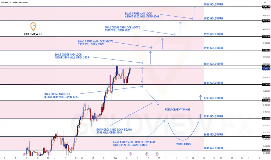
GOLD 4H CHART ROUTE MAP UPDATE & TRADING PLAN FOR THE WEEKHey Everyone,
Please see our updated 4h chart levels and targets for the coming week.
We are seeing price play between two weighted levels with a gap above at 3894 and a gap below at 3839. We will need to see ema5 cross and lock on either weighted level to determine the next range.
We will see levels tested side by side until one of the weighted levels break and lock to confirm direction for the next range.
We will keep the above in mind when taking buys from dips. Our updated levels and weighted levels will allow us to track the movement down and then catch bounces up.
We will continue to buy dips using our support levels taking 20 to 40 pips. As stated before each of our level structures give 20 to 40 pip bounces, which is enough for a nice entry and exit. If you back test the levels we shared every week for the past 24 months, you can see how effectively they were used to trade with or against short/mid term swings and trends.
The swing range give bigger bounces then our weighted levels that's the difference between weighted levels and swing ranges.
BULLISH TARGET
3894
EMA5 CROSS AND LOCK ABOVE 3894 WILL OPEN THE FOLLOWING BULLISH TARGETS
3939
EMA5 CROSS AND LOCK ABOVE 3939 WILL OPEN THE FOLLOWING BULLISH TARGET
3979
EMA5 CROSS AND LOCK ABOVE 3979 WILL OPEN THE FOLLOWING BULLISH TARGET
4025
EMA5 CROSS AND LOCK ABOVE 4025 WILL OPEN THE FOLLOWING BULLISH TARGET
4066
BEARISH TARGETS
3839
EMA5 CROSS AND LOCK BELOW 3793 WILL OPEN THE FOLLOWING BEARISH TARGET
3741
EMA5 CROSS AND LOCK BELOW 3741 WILL OPEN THE SWING RANGE
3688
3648
As always, we will keep you all updated with regular updates throughout the week and how we manage the active ideas and setups. Thank you all for your likes, comments and follows, we really appreciate it!
Mr Gold
GoldViewFX
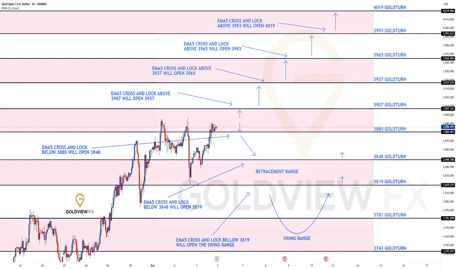
GOLD 1H CHART ROUTE MAP UPDATE & TRADING PLAN FOR THE WEEKHey Everyone,
Please see our updated 1h chart levels and targets for the coming week.
We are seeing price play between two weighted levels with a gap above at 3907 and a gap below at 3880. We will need to see ema5 cross and lock on either weighted level to determine the next range.
We will see levels tested side by side until one of the weighted levels break and lock to confirm direction for the next range.
We will keep the above in mind when taking buys from dips. Our updated levels and weighted levels will allow us to track the movement down and then catch bounces up.
We will continue to buy dips using our support levels taking 20 to 40 pips. As stated before each of our level structures give 20 to 40 pip bounces, which is enough for a nice entry and exit. If you back test the levels we shared every week for the past 24 months, you can see how effectively they were used to trade with or against short/mid term swings and trends.
The swing range give bigger bounces then our weighted levels that's the difference between weighted levels and swing ranges.
BULLISH TARGET
3907
EMA5 CROSS AND LOCK ABOVE 3907 WILL OPEN THE FOLLOWING BULLISH TARGETS
3937
EMA5 CROSS AND LOCK ABOVE 3937 WILL OPEN THE FOLLOWING BULLISH TARGET
3965
EMA5 CROSS AND LOCK ABOVE 3965 WILL OPEN THE FOLLOWING BULLISH TARGET
3993
EMA5 CROSS AND LOCK ABOVE 3993 WILL OPEN THE FOLLOWING BULLISH TARGET
4019
BEARISH TARGETS
3880
EMA5 CROSS AND LOCK BELOW 3880 WILL OPEN THE FOLLOWING BEARISH TARGET
3848
EMA5 CROSS AND LOCK BELOW 3848 WILL OPEN THE FOLLOWING BEARISH TARGET
3819
EMA5 CROSS AND LOCK BELOW 3819 WILL OPEN THE SWING RANGE
3781
3743
As always, we will keep you all updated with regular updates throughout the week and how we manage the active ideas and setups. Thank you all for your likes, comments and follows, we really appreciate it!
Mr Gold
GoldViewFX
Is Your Money Safe in the Global Market?Introduction: Understanding Global Market Safety
In today’s interconnected financial world, investors from all corners of the globe participate in markets that span continents, currencies, and asset classes. From equities in New York and bonds in London to commodities in Dubai and emerging market funds in Asia — the global marketplace offers immense opportunities for growth. However, with great opportunity comes great risk. The question that often arises is: “How do I know my money is safe in the global market?”
Financial safety doesn’t mean avoiding risks entirely — it means understanding, managing, and minimizing them while ensuring that your wealth is protected from volatility, fraud, inflation, and geopolitical uncertainty. In this comprehensive guide, we’ll explore how to assess the safety of your investments, the factors influencing market stability, and practical steps to safeguard your money in the international financial system.
1. The Concept of Financial Safety in a Global Context
Before diving into protection strategies, it’s crucial to understand what “safety” means in the context of global markets. Investment safety can be broken down into several layers:
Capital Preservation: Ensuring your principal investment is not lost due to volatility or fraud.
Liquidity: Having the ability to convert your investments into cash without excessive losses.
Diversification: Spreading investments across regions and asset classes to minimize exposure to localized risks.
Regulatory Security: Investing under well-regulated jurisdictions that protect investors through strong legal frameworks.
Transparency: Having access to reliable information about the companies, governments, or institutions managing your money.
Safety doesn’t imply zero risk — it’s about making informed, balanced decisions in a world where both risks and rewards coexist.
2. Identifying Risks in the Global Market
Understanding where potential threats lie is the first step toward protecting your capital. Key global market risks include:
a. Market Volatility
Prices of stocks, commodities, and currencies fluctuate due to investor sentiment, economic data, and political events. Sudden crashes or corrections can erode investment value.
b. Currency Risk
Exchange rate fluctuations can significantly impact returns for investors holding assets denominated in foreign currencies.
c. Geopolitical Risk
Wars, sanctions, trade restrictions, and political instability can destabilize entire regions, affecting investments globally.
d. Inflation and Interest Rate Risk
Central banks across the world control monetary policy, and their decisions on interest rates can influence global asset prices and investor returns.
e. Corporate and Credit Risk
When investing in international bonds or equities, there’s a possibility that companies or governments might default or underperform.
f. Cybersecurity and Fraud Risk
In the digital age, online trading and fintech platforms are vulnerable to hacking and scams. Protecting your accounts and verifying platforms are critical steps.
By understanding these threats, investors can take strategic steps to defend against them.
3. How to Assess the Safety of Global Investments
To determine whether your money is safe, use a multi-dimensional approach. Ask yourself the following questions before investing:
a. Who Regulates the Platform or Institution?
Ensure the financial institution is licensed under credible authorities like the U.S. SEC, UK FCA, or Monetary Authority of Singapore (MAS). These regulators impose strict rules to protect investors.
b. What is the Level of Transparency?
Trustworthy institutions publish audited financial statements and disclose their operations clearly. Lack of transparency is a red flag.
c. How Liquid Are My Investments?
Can you easily sell your assets or withdraw your funds? Illiquid markets can trap investors during crises.
d. What is the Risk Profile of the Asset Class?
Stocks, bonds, commodities, and cryptocurrencies all carry different risk levels. Balancing them according to your goals ensures stability.
e. How Diversified Is My Portfolio?
Investing across regions, sectors, and asset types minimizes exposure to localized risks.
f. Is There Insurance or Protection?
Check if your investments are covered by schemes like FDIC insurance (U.S.), Investor Compensation Scheme (U.K.), or equivalent programs in other countries.
4. The Role of Diversification in Safeguarding Money
Diversification is the cornerstone of global financial safety. By spreading investments across:
Geographies (U.S., Europe, Asia, Emerging Markets)
Asset Classes (Stocks, Bonds, Gold, Real Estate, Mutual Funds, ETFs)
Currencies (USD, EUR, GBP, JPY, INR, etc.)
…you can reduce the impact of any one region or market downturn. For example, when U.S. stocks fall, gold or Asian markets may rise, balancing your portfolio.
A well-diversified portfolio doesn’t guarantee profits, but it reduces the likelihood of catastrophic losses — ensuring long-term sustainability.
5. Importance of Financial Regulation and Investor Protection
Global financial safety relies heavily on regulatory systems. Reputable markets have robust laws to ensure:
Transparency and disclosure
Investor compensation in case of fraud
Clear operational standards for brokers and fund managers
Protection against insider trading and manipulation
When choosing a platform or institution, verify its regulatory license. Always invest through brokers and fund houses that are registered with major global regulatory authorities.
Avoid unregulated platforms that promise unrealistic returns — these are often scams or Ponzi schemes.
6. The Role of Technology and Cybersecurity in Financial Safety
Modern investing heavily depends on online trading platforms, mobile apps, and digital wallets. While technology provides convenience, it also introduces cyber risks.
To keep your investments safe:
Use two-factor authentication (2FA) on all trading accounts.
Never share passwords or OTPs.
Avoid public Wi-Fi while accessing trading apps.
Regularly monitor account statements for suspicious activities.
Ensure your broker uses end-to-end encryption and regulated payment gateways.
Financial cybersecurity is not just a company’s responsibility — it’s also a personal discipline.
7. Safe Haven Assets and Hedging Strategies
During global uncertainty — such as recessions, wars, or inflation spikes — investors often move their capital into safe haven assets, which tend to retain value.
These include:
Gold: A timeless hedge against inflation and currency devaluation.
U.S. Treasury Bonds: Considered among the safest investments globally.
Swiss Franc (CHF): A historically stable currency.
Blue-chip Stocks: Established multinational companies with strong fundamentals.
Hedging techniques like currency hedging, options, and futures can also protect against downside risks in volatile markets.
8. Evaluating the Global Economic Environment
Keeping your money safe requires staying informed about macroeconomic trends. Watch for:
Central bank policies (interest rates, quantitative easing)
Inflation data and GDP growth rates
Trade balances and foreign exchange reserves
Corporate earnings reports
A global investor must think beyond local borders — a policy shift in Washington or Beijing can influence markets from Mumbai to London.
9. Psychological Safety: The Human Element in Investing
Emotional decision-making often leads to poor investment choices. Fear and greed drive volatility more than data does. To ensure your money remains safe:
Avoid impulsive trading during market crashes.
Stick to a disciplined investment plan.
Set clear stop-loss levels and profit targets.
Regularly review and rebalance your portfolio.
Remember, the most dangerous element in investing isn’t the market — it’s the investor’s reaction to it.
10. Long-Term vs. Short-Term Safety
Short-term safety focuses on liquidity and minimizing volatility — ideal for emergency funds or near-term goals.
Long-term safety depends on inflation-beating growth through strategic diversification.
Balancing both ensures you don’t just protect your money — you grow it steadily over time.
11. The Future of Financial Safety: AI, Blockchain, and Transparency
Emerging technologies are redefining investment safety:
Blockchain ensures transparent and tamper-proof transactions.
Artificial Intelligence (AI) helps in fraud detection and portfolio optimization.
Decentralized Finance (DeFi) platforms are creating new ways for secure global investments — though they carry new types of risks.
The future of financial safety will be shaped by technology-led transparency, enabling investors to make more secure decisions globally.
12. Steps to Ensure Your Money Is Safe in the Global Market
Here’s a practical checklist every investor should follow:
Choose regulated brokers or financial institutions.
Diversify across asset classes and regions.
Use strong cybersecurity measures.
Avoid high-return, low-transparency schemes.
Monitor your investments regularly.
Stay informed about global macroeconomic trends.
Have an exit strategy and emergency plan.
Seek advice from certified financial advisors.
Financial safety is not a one-time act — it’s a continuous process of education, vigilance, and adaptation.
Conclusion: Security Through Knowledge and Strategy
The global financial market will always carry a mix of risk and reward. True safety doesn’t lie in avoiding risk entirely but in understanding and managing it wisely. By staying informed, diversifying strategically, using regulated platforms, and leveraging technology responsibly, investors can ensure that their money remains protected — no matter how volatile or uncertain the global landscape becomes.
In essence, your money’s safety depends not just on where you invest, but how you invest. With discipline, awareness, and smart planning, your wealth can thrive securely in the ever-evolving global marketplace.

Exploring the Types of Global Trading1. What is Global Trading?
Global trading refers to the exchange of goods, services, and financial assets between countries. It encompasses import and export activities, investment flows, and financial transactions that cross national borders. This system is the foundation of globalization — connecting producers and consumers across continents, creating job opportunities, and promoting economic efficiency.
It allows countries to:
Access goods and services not produced domestically.
Utilize comparative advantages.
Boost productivity through specialization.
Strengthen diplomatic and economic relationships.
2. The Evolution of Global Trading
Global trade has evolved over centuries — from the ancient Silk Road to today’s digital trade platforms. The journey reflects how innovation, technology, and political agreements have shaped economic interdependence.
Ancient Trade (Pre-1500s): Exchange of spices, textiles, and metals through trade routes like the Silk Road and maritime trade networks.
Colonial Era (1500s–1800s): Expansion of European empires led to global trade in commodities, often through exploitative systems.
Industrial Revolution (1800s–1900s): Mechanization and mass production boosted exports and international shipping.
Modern Era (1900s–Present): Rise of multinational corporations, free trade agreements, and digital commerce.
Today, global trading operates in multiple dimensions — involving physical goods, services, capital markets, and data exchange — with technology acting as a catalyst for rapid transactions and global supply chains.
3. Major Types of Global Trading
Global trading can be categorized based on the nature of exchange, mode of transaction, and economic objective. Let’s explore each type in detail.
A. Trade in Goods (Merchandise Trade)
This is the most traditional and visible form of trade. It includes tangible products that move across borders — raw materials, manufactured goods, consumer products, and industrial equipment.
Examples:
Crude oil exports from Saudi Arabia.
Electronics exports from South Korea and China.
Agricultural imports like wheat or soybeans by developing nations.
Subcategories:
Primary Goods: Raw materials and agricultural products.
Manufactured Goods: Industrial and consumer products like cars, electronics, and clothing.
Intermediate Goods: Components used in manufacturing final products (e.g., semiconductors).
Significance:
Trade in goods accounts for a major portion of world trade volume and reflects the industrial and resource strengths of nations.
B. Trade in Services
Unlike physical goods, service trade involves intangible offerings — consulting, tourism, IT, education, and financial services.
Examples:
India’s IT outsourcing services to U.S. companies.
Tourism in France and Thailand.
Financial services provided by London and Singapore.
Features:
Requires skilled labor and digital connectivity.
Less dependent on physical logistics.
Plays a crucial role in developed economies.
Impact:
The global services trade has grown rapidly due to digitalization, allowing even small firms to provide services internationally via the internet.
C. Capital and Financial Trading
This involves the movement of money and investments across borders. Investors buy and sell financial assets, currencies, or equity stakes in foreign companies.
Types:
Foreign Direct Investment (FDI): Long-term investment in foreign enterprises.
Foreign Portfolio Investment (FPI): Short-term investments in stocks, bonds, or securities.
Currency Trading (Forex): Exchange of global currencies for profit or hedging.
Sovereign Investments: Governments investing in global assets.
Importance:
Capital trading ensures the efficient allocation of financial resources globally, supports business expansion, and stabilizes economic growth.
D. E-commerce and Digital Trade
In the modern era, digitalization has transformed global trade. E-commerce enables businesses to sell goods and services worldwide without physical presence, while digital trade includes cross-border data, software, and online services.
Examples:
Amazon and Alibaba operating globally.
Freelance platforms like Upwork and Fiverr connecting clients and workers worldwide.
Streaming services and digital content exports.
Advantages:
Low transaction costs.
Broader market access for SMEs.
Instant payments and logistics integration.
Challenges:
Data privacy concerns.
Cybersecurity threats.
Regulatory differences across countries.
E. Commodity Trading
Commodities are basic goods used in commerce — such as metals, energy, and agricultural products. Commodity trading occurs through exchanges like the London Metal Exchange (LME) or Chicago Mercantile Exchange (CME).
Categories:
Energy Commodities: Oil, natural gas, coal.
Metals: Gold, silver, copper, aluminum.
Agricultural Commodities: Wheat, sugar, coffee, cotton.
Why It Matters:
Commodity prices influence inflation, industrial costs, and the overall stability of national economies.
F. Derivatives and Financial Instruments Trading
Global financial markets also involve trading in derivatives, which are contracts based on the value of an underlying asset (like stocks, commodities, or currencies).
Common Types:
Futures and Options
Swaps and Forwards
Index derivatives
Purpose:
Hedging against market volatility.
Speculative profits.
Portfolio diversification.
Example:
Traders in the U.S. may use futures contracts to hedge against oil price fluctuations, while investors in Japan may use currency derivatives to protect export earnings.
G. Intra-Industry and Inter-Industry Trade
Inter-Industry Trade: Exchange of goods belonging to different industries (e.g., cars for textiles).
Intra-Industry Trade: Exchange of similar goods between countries (e.g., Japan and Germany trading different car models).
Why It Happens:
Due to specialization, technology variations, and consumer preferences for diversity.
H. Fair Trade and Ethical Trading
An increasingly important type of trade focuses on ethical sourcing, ensuring fair wages, environmental sustainability, and human rights protection.
Examples:
Fair-trade coffee and cocoa.
Eco-friendly textiles.
Ethical diamond sourcing.
Impact:
Encourages sustainable economic development, especially in developing nations.
4. Benefits of Global Trading
Economic Growth: Expands GDP and income levels through exports and investments.
Job Creation: Boosts employment across sectors, from manufacturing to logistics.
Innovation: Encourages technological transfer and competitive improvement.
Consumer Benefits: Provides access to diverse products at competitive prices.
Political Stability: Strengthens international cooperation and alliances.
Efficiency: Enables countries to focus on industries where they have a comparative advantage.
5. Challenges in Global Trading
Despite its advantages, global trading faces several obstacles:
Trade Barriers: Tariffs, quotas, and sanctions limit free trade.
Currency Fluctuations: Exchange rate volatility affects profits and prices.
Supply Chain Disruptions: Events like pandemics or wars can halt global logistics.
Political Risks: Diplomatic tensions and protectionism influence global markets.
Environmental Concerns: High carbon emissions from shipping and production.
Digital Divide: Not all nations benefit equally from e-commerce and digital trade.
6. The Role of Trade Agreements and Organizations
International organizations and trade agreements play a key role in promoting fair and open trade.
Major Institutions:
World Trade Organization (WTO)
International Monetary Fund (IMF)
World Bank
OECD
Regional Trade Blocs like ASEAN, EU, and NAFTA (USMCA)
Purpose:
Standardize rules.
Resolve trade disputes.
Promote development and investment.
7. Future of Global Trading
The future of global trading is shaped by technology, sustainability, and geopolitical shifts.
Emerging Trends:
Artificial Intelligence in Trade Analytics
Blockchain for Transparent Supply Chains
Sustainable and Green Trade Policies
Rise of Regional Trade Agreements
Digital Currencies in Cross-Border Payments
As automation, AI, and digital currencies redefine global commerce, adaptability will determine which nations and businesses lead in the next generation of global trade.
8. Conclusion
Global trading is far more than an exchange of goods — it’s an intricate system of economic relationships that shapes nations’ destinies. From tangible commodities to intangible data flows, from multinational corporations to small digital entrepreneurs — every participant contributes to this dynamic global ecosystem.
Understanding the types of global trading empowers investors, policymakers, and businesses to make informed decisions, minimize risks, and seize new opportunities. As the world becomes increasingly interconnected, the essence of trade continues to evolve — emphasizing innovation, fairness, and sustainability.
In the coming decades, those who understand and adapt to these diverse forms of global trading will not just survive — they will lead the future of the global economy.
Master Correlation StrategiesUnlocking the Power of Inter-Market Relationships in Trading.
1. Understanding Correlation in Trading
Correlation refers to the statistical relationship between two or more financial instruments — how their prices move relative to each other. It is expressed through a correlation coefficient ranging from -1 to +1.
Positive Correlation (+1): When two assets move in the same direction. For example, crude oil and energy sector stocks often rise and fall together.
Negative Correlation (-1): When two assets move in opposite directions. For instance, the U.S. dollar and gold often have an inverse relationship — when one rises, the other tends to fall.
Zero Correlation (0): Indicates no consistent relationship between two assets.
Understanding these relationships helps traders predict how one market might respond based on the movement of another, enhancing decision-making and portfolio design.
2. Why Correlation Matters
In modern financial markets, where globalization links commodities, equities, currencies, and bonds, no asset class operates in isolation. Correlation strategies allow traders to see the “bigger picture” — understanding how shifts in one area of the market ripple across others.
Some key reasons why correlation is vital include:
Risk Management: Diversification is only effective when assets are uncorrelated. If all your holdings move together, your portfolio is not truly diversified.
Predictive Analysis: Monitoring correlated assets helps anticipate price moves. For example, a rally in crude oil might foreshadow gains in oil-dependent currencies like the Canadian Dollar (CAD).
Hedging Opportunities: Traders can offset risks by holding negatively correlated assets. For instance, pairing long stock positions with short positions in an inverse ETF.
Market Confirmation: Correlations can validate or contradict signals. If gold rises while the dollar weakens, the move is more credible than when both rise together, which is rare.
3. Core Types of Correlations in Markets
a. Intermarket Correlation
This examines how different asset classes relate — such as the link between commodities, bonds, currencies, and equities. For example:
Rising interest rates typically strengthen the domestic currency but pressure stock prices.
Falling bond yields often boost equity markets.
b. Intra-market Correlation
This focuses on assets within the same category. For example:
Technology sector stocks often move together based on broader industry trends.
Gold and silver tend to share similar price patterns.
c. Cross-Asset Correlation
This involves analyzing relationships between assets of different types, such as:
Gold vs. U.S. Dollar
Crude Oil vs. Inflation Expectations
Bitcoin vs. NASDAQ Index
d. Temporal Correlation
Certain correlations shift over time. For instance, the correlation between equities and bonds may be positive during economic growth and negative during recessions.
4. Tools and Techniques to Measure Correlation
Correlation is not merely an observation—it’s a quantifiable concept. Several statistical tools help traders measure and monitor it accurately.
a. Pearson Correlation Coefficient
This is the most widely used formula to calculate linear correlation between two data sets. A reading close to +1 or -1 shows a strong relationship, while values near 0 indicate weak correlation.
b. Rolling Correlation
Markets evolve constantly, so rolling correlation (using moving windows) helps identify how relationships shift over time. For example, a 30-day rolling correlation between gold and the USD can show whether their inverse relationship is strengthening or weakening.
c. Correlation Matrices
These are tables showing the correlation coefficients between multiple assets at once. Portfolio managers use them to construct diversified portfolios and reduce overlapping exposures.
d. Software Tools
Platforms like Bloomberg Terminal, TradingView, MetaTrader, and Python-based tools (like pandas and NumPy libraries) allow traders to calculate and visualize correlation efficiently.
5. Applying Correlation Strategies in Trading
a. Pair Trading
Pair trading is a market-neutral strategy that exploits temporary deviations between two historically correlated assets.
Example:
If Coca-Cola and Pepsi usually move together, but Pepsi lags temporarily, traders may go long Pepsi and short Coca-Cola, betting the relationship will revert.
b. Hedging with Negative Correlations
Traders can use negatively correlated instruments to offset risk. For instance:
Long positions in the stock market can be hedged by taking positions in safe-haven assets like gold or the Japanese Yen.
c. Sector Rotation and ETF Strategies
Investors track sector correlations with broader indices to identify leading and lagging sectors.
For example:
If financial stocks start outperforming the S&P 500, this could signal a shift in the economic cycle.
d. Currency and Commodity Correlations
Currencies are deeply linked to commodities:
The Canadian Dollar (CAD) often correlates positively with crude oil prices.
The Australian Dollar (AUD) correlates with gold and iron ore prices.
The Swiss Franc (CHF) is often inversely correlated with global risk sentiment, acting as a safe haven.
Traders can exploit these relationships for cross-market opportunities.
6. Case Studies of Correlation in Action
a. Gold and the U.S. Dollar
Gold is priced in dollars; therefore, when the USD strengthens, gold usually weakens as it becomes more expensive for other currency holders.
During 2020’s pandemic uncertainty, both assets briefly rose together — a rare situation showing correlation can shift temporarily under stress.
b. Oil Prices and Inflation
Oil serves as a barometer for inflation expectations. When crude prices rise, inflation fears grow, prompting central banks to tighten policies.
Traders who monitor this relationship can anticipate policy shifts and market reactions.
c. Bitcoin and Tech Stocks
In recent years, Bitcoin has shown increasing correlation with high-growth technology stocks. This suggests that cryptocurrency markets are influenced by risk sentiment similar to the equity market.
7. Benefits of Mastering Correlation Strategies
Enhanced Market Insight: Understanding inter-market dynamics reveals the underlying forces driving price movements.
Stronger Portfolio Construction: Diversify effectively by choosing assets that truly offset one another.
Smarter Risk Control: Correlation analysis highlights hidden exposures across asset classes.
Improved Trade Timing: Correlation signals help confirm or challenge technical and fundamental setups.
Global Perspective: By studying correlations, traders gain insight into how global events ripple through interconnected markets.
8. Challenges and Limitations
Despite its power, correlation analysis is not foolproof. Traders must be aware of its limitations:
Changing Relationships: Correlations evolve over time due to policy changes, crises, or shifting investor sentiment.
False Correlation: Sometimes two assets appear correlated by coincidence without a fundamental link.
Lag Effect: Correlation may not capture time delays between cause and effect across markets.
Overreliance: Correlation is one tool among many; combining it with technical, fundamental, and sentiment analysis produces more reliable outcomes.
9. Advanced Correlation Techniques
a. Cointegration
While correlation measures relationships at a moment in time, cointegration identifies long-term equilibrium relationships between two non-stationary price series.
For example, even if short-term correlation fluctuates, two assets can remain cointegrated over the long run — useful in statistical arbitrage.
b. Partial Correlation
This method isolates the relationship between two variables while controlling for others. It’s particularly helpful in complex portfolios involving multiple correlated instruments.
c. Dynamic Conditional Correlation (DCC) Models
These advanced econometric models (used in quantitative finance) measure time-varying correlations — essential for modern algorithmic trading systems.
10. Building a Correlation-Based Trading System
A professional correlation strategy can be structured as follows:
Data Collection: Gather historical price data for multiple assets.
Statistical Analysis: Calculate correlations and rolling relationships using software tools.
Strategy Design: Develop pair trades, hedges, or intermarket signals based on correlation thresholds.
Backtesting: Validate the system across different market phases to ensure robustness.
Execution and Monitoring: Continuously update correlation data and adjust positions as relationships evolve.
Risk Control: Implement stop-loss rules and diversification limits to prevent overexposure to correlated positions.
11. The Future of Correlation Strategies
In an era of high-frequency trading, AI-driven analytics, and global macro interconnectedness, correlation strategies are evolving rapidly. Machine learning models now identify non-linear and hidden correlations that traditional statistics might miss.
Furthermore, as markets integrate further — with crypto, ESG assets, and alternative data sources entering the scene — understanding these new correlations will be crucial for maintaining an edge in trading.
12. Final Thoughts
Mastering correlation strategies isn’t just about mathematics — it’s about understanding the language of global markets. Every movement in commodities, currencies, and indices tells a story about how capital flows across the world.
A trader who comprehends these relationships gains not only analytical power but also strategic foresight. By mastering correlation analysis, you move beyond isolated price charts and see the interconnected web that drives the global financial ecosystem.
In essence, correlation strategies are the bridge between micro-level technical trades and macro-level economic understanding. Those who can navigate this bridge with confidence stand at the forefront of modern trading excellence — armed with knowledge, precision, and an unshakable sense of market direction.
Global Trading News: No More Noise1. The Problem: Too Much Noise, Too Little Clarity
In the age of digital speed, financial information travels faster than ever before. Every second, thousands of updates pour in from stock exchanges, economic data feeds, and social media platforms. While access to this information is crucial, the real challenge is filtering signal from noise.
For traders and investors, the consequences of acting on misleading or incomplete data can be severe—ranging from missed opportunities to significant financial losses. Many find themselves reacting emotionally to market movements rather than making rational, data-driven decisions.
Here’s the reality of modern trading news:
Information overload: The average trader consumes 10x more data today than they did a decade ago.
Unverified sources: Social platforms and influencer-driven “news” often spread unconfirmed rumors.
Delayed reactions: By the time mainstream media reports an event, the market has often already moved.
Conflicting analysis: Multiple experts giving contradictory opinions can paralyze decision-making.
This environment creates a noise-heavy ecosystem, where clarity is lost and focus diluted. That’s why the future of global trading depends not just on access to data—but on access to refined, verified, and context-driven insights.
2. The Concept: No More Noise – Only Insight
“Global Trading News: No More Noise” is more than a headline—it’s a mindset shift. It’s about transforming how traders receive and process global market updates. Instead of drowning in endless feeds, this approach focuses on precision, context, and credibility.
a. Filtered Information Flow
Instead of providing every minor update, this system curates only market-moving news—those that have a proven impact on price action or sentiment. Macro-economic indicators, central bank decisions, corporate earnings, geopolitical shifts, and commodity trends are prioritized.
b. Data-Driven Analysis
News without numbers is just noise. Each report is paired with relevant data visualization—charts, volume trends, volatility indexes, and correlation patterns—so traders can instantly see the real market effect behind the headline.
c. AI-Powered News Screening
Using intelligent algorithms, irrelevant or repetitive information is filtered out. The AI recognizes patterns of manipulation, misinformation, or algorithmic pumping stories, keeping the feed credible and clean.
d. Real-Time Global Coverage
From New York to Tokyo, from London to Mumbai—the platform ensures 24/7 coverage of major exchanges, currencies, bonds, commodities, and crypto markets. But unlike traditional platforms, the content is localized yet globalized—tailored to highlight how a move in one market impacts another.
3. The Mission: Empower the Modern Trader
At the core of “Global Trading News: No More Noise” lies a simple mission—to empower every trader and investor with information that matters. In financial markets, clarity equals confidence, and confidence leads to smarter, faster decisions.
Key Objectives:
Simplify complexity: Break down macroeconomic data into clear trading insights.
Enhance focus: Remove distractions and highlight what truly moves markets.
Increase speed: Provide verified insights in real-time for instant action.
Build trust: Ensure every piece of information is credible, sourced, and traceable.
Whether you’re a day trader chasing volatility, a swing trader identifying trends, or an institutional investor managing global portfolios, the goal is the same—make decisions based on facts, not fear or noise.
4. The Framework: How “No More Noise” Works
The global financial world can be divided into multiple verticals—equities, currencies, commodities, bonds, and digital assets. Each responds differently to macro events. The “No More Noise” system organizes news through a five-layer structure designed for clarity and precision.
Layer 1: Macro Alerts
Tracks and analyzes central bank policies, inflation data, GDP numbers, and geopolitical shifts. Example: “Federal Reserve holds rates steady amid inflation uncertainty—market expects pivot by Q1.”
Layer 2: Market Movers
Covers stocks, commodities, and currency pairs that show significant volume spikes or trend reversals due to fundamental news or institutional activity.
Layer 3: Sector Insights
Focuses on industries driving momentum—tech, energy, metals, banking, and pharmaceuticals—linking global developments to sectoral performance.
Layer 4: Quant & Sentiment Tools
Integrates market sentiment analysis, correlation tracking, and volatility forecasting to help traders validate the emotional tone behind the news.
Layer 5: Strategic Analysis
Provides commentary from credible financial analysts and economists—offering deeper interpretations rather than just surface-level reporting.
5. The Impact: Transforming Trading Behavior
When traders are freed from noise, their behavior changes dramatically:
Reduced overtrading: Decisions become data-backed instead of emotional.
Improved accuracy: Clearer insights lead to better entry and exit timing.
Enhanced portfolio management: Macro and micro factors are balanced effectively.
Stronger confidence: Traders operate with purpose, not panic.
Moreover, by prioritizing quality over quantity, traders save time—turning market monitoring into a strategic edge rather than a distraction.
6. Global Connectivity, Local Relevance
What makes global trading unique today is interconnectivity. A bond yield movement in the U.S. can impact Asian equities; a commodity rally in London can influence Indian inflation data. “Global Trading News: No More Noise” focuses on showing these interlinkages in real-time, allowing traders to:
Understand global cause-and-effect relationships.
Anticipate market reactions before they happen.
Diversify their trading strategies across regions and asset classes.
This creates a borderless trading mindset, where every event—no matter where it originates—is understood through a global lens.
7. The Future: Intelligent, Calm, and Data-Driven Markets
As artificial intelligence, blockchain data feeds, and quantum computing evolve, the future of trading will rely on smart filtering systems. The age of raw information is ending—the age of interpreted intelligence is beginning.
The traders who adapt to this evolution will thrive, not by consuming more, but by understanding better.
“Global Trading News: No More Noise” represents this shift—towards mindful trading, where every click, trade, and reaction is intentional and informed.
In this future, financial media platforms will no longer compete on who delivers the news first—but on who delivers it right. The market will reward depth over drama, insight over intensity, and facts over frenzy.
8. Why This Matters Now
In volatile times—whether it’s global inflation, war tensions, or digital currency disruption—the margin for error in trading decisions is smaller than ever. Every second counts, and every false signal costs. That’s why news quality has become the new competitive advantage.
“Global Trading News: No More Noise” isn’t just a tagline—it’s a philosophy for the next generation of market thinkers who value truth, timing, and transparency over hype.
Conclusion: The New Era of Trading Clarity
The global market doesn’t need more information—it needs better information.
In an age where every second brings a new headline, clarity is the ultimate trading edge.
“Global Trading News: No More Noise” is a commitment to restore that edge—to make traders think smarter, act faster, and trade with conviction. It’s where insight replaces speculation, and where news becomes a tool for empowerment, not confusion.
In this silent revolution of clarity, the markets may still be loud—but the trader will remain calm, focused, and informed.
Because when there’s no more noise, there’s nothing left but the truth—and in trading, truth is power.

Currency Convertibility Issues in the Global MarketIntroduction
Currency convertibility is one of the fundamental pillars of the global financial system. It determines how freely a nation’s currency can be exchanged for foreign currencies, influencing trade, investment, and international economic stability. In a world increasingly interconnected through globalization, the concept of currency convertibility is central to understanding how nations engage in global commerce and finance. However, the issue of currency convertibility is complex and often tied to a country’s monetary policy, balance of payments, capital control measures, and overall economic health.
This essay explores the concept of currency convertibility in the global market, its types, significance, challenges, and the major issues that affect countries’ decisions to make their currencies fully convertible. It also examines case studies of economies that have struggled or succeeded with convertibility and provides an outlook on how currency convertibility impacts the global financial ecosystem.
1. Meaning of Currency Convertibility
Currency convertibility refers to the ease with which a country’s currency can be converted into another currency or gold. It represents the degree of freedom that individuals, businesses, and investors have in exchanging domestic currency for foreign currencies for trade, investment, or travel purposes.
Essentially, convertibility is an indicator of how open an economy is to international financial flows. When a currency is fully convertible, it can be freely exchanged without restrictions for any purpose. When it is partially convertible, certain limitations exist—usually to control capital outflow or to stabilize the domestic economy.
2. Types of Currency Convertibility
Currency convertibility is generally categorized into two main types:
a. Current Account Convertibility
This allows the exchange of domestic currency for foreign currency for trade in goods and services, interest payments, and remittances. It ensures smooth international trade and reflects a country’s openness to global commerce.
Most nations, including India, have achieved current account convertibility. This means residents can pay for imports or receive export payments in foreign currencies freely.
b. Capital Account Convertibility
This involves the freedom to convert domestic financial assets into foreign assets and vice versa. It allows unrestricted movement of capital across borders—such as investment in foreign stocks, bonds, real estate, or repatriation of profits.
While this form of convertibility attracts foreign direct investment (FDI) and portfolio flows, it can also expose the domestic economy to external shocks and speculative capital movements.
3. Importance of Currency Convertibility in the Global Market
Currency convertibility plays a vital role in integrating national economies into the global system. Its importance can be highlighted through several key dimensions:
Facilitating International Trade:
Convertibility enables smooth cross-border transactions, reducing transaction costs and delays. Exporters and importers can easily settle payments in international currencies like the US dollar or euro.
Encouraging Foreign Investment:
Foreign investors prefer investing in economies where they can easily convert their earnings into other currencies. Full convertibility signals economic openness and financial maturity.
Enhancing Market Confidence:
A convertible currency reflects the stability and credibility of a nation’s monetary policy. It builds confidence among traders, investors, and international partners.
Improving Resource Allocation:
When funds can flow freely across borders, resources are allocated more efficiently, and economies can tap into global capital pools.
Promoting Globalization:
Convertibility supports global integration, allowing citizens and companies to participate more actively in the international economy.
4. Challenges and Risks of Currency Convertibility
While currency convertibility brings several advantages, it also presents significant challenges and risks, especially for developing economies.
a. Exchange Rate Volatility
Full convertibility can expose a nation’s currency to global market fluctuations. Speculative attacks and sudden changes in capital flows can destabilize the exchange rate, leading to inflationary pressures or currency depreciation.
b. Capital Flight
When investors lose confidence in a country’s economy, unrestricted capital convertibility can lead to massive capital outflows. This can drain foreign exchange reserves and weaken the domestic currency.
c. Loss of Monetary Control
With full capital account convertibility, central banks may find it difficult to manage monetary policy effectively, as large inflows and outflows can disrupt domestic liquidity and interest rates.
d. External Shocks
Global crises, such as the 2008 financial meltdown, highlight how interconnected financial markets can transmit risks rapidly. Countries with fully convertible currencies may face contagion effects more severely.
e. Inflation and Economic Instability
Sudden currency depreciation due to speculative pressures can raise import costs, leading to inflation and economic instability, particularly in countries dependent on imports for essential goods.
5. Case Studies: Global Experiences with Currency Convertibility
a. India
India has achieved current account convertibility since 1994 but still maintains partial capital account convertibility. The Reserve Bank of India (RBI) exercises control over capital flows to prevent volatility and speculative attacks. The cautious approach helped India withstand crises such as the Asian Financial Crisis (1997) and the Global Financial Crisis (2008).
b. China
China’s yuan (CNY) has been gradually moving toward greater convertibility. While trade-related transactions are largely convertible, capital account restrictions remain. China maintains tight control over capital flows to manage its exchange rate and protect economic stability.
c. Argentina
Argentina’s experience serves as a cautionary tale. In the 1990s, it adopted full convertibility by pegging its currency to the US dollar. While initially stabilizing inflation, it later led to economic collapse due to inflexible policies, capital flight, and loss of competitiveness.
d. Developed Economies (U.S., U.K., Eurozone)
Fully convertible currencies like the US Dollar, Euro, and British Pound dominate global trade and finance. Their stable economies, robust institutions, and deep financial markets enable them to sustain full convertibility with minimal disruption.
6. The Role of International Institutions
International organizations like the International Monetary Fund (IMF) and the World Bank play crucial roles in guiding countries toward managed currency convertibility.
The IMF’s Article VIII encourages member nations to remove restrictions on current account transactions but advises caution regarding capital account liberalization. It promotes gradual, sequenced reforms to avoid destabilizing the economy.
7. Factors Influencing a Country’s Currency Convertibility Decision
A nation’s decision to move toward full convertibility depends on several economic and political factors:
Macroeconomic Stability:
Low inflation, sustainable fiscal deficits, and stable growth are prerequisites for safe convertibility.
Foreign Exchange Reserves:
Adequate reserves ensure that the country can handle fluctuations in capital flows.
Financial Market Depth:
Developed financial markets can absorb capital movements efficiently without destabilizing the economy.
Exchange Rate Regime:
Flexible exchange rate systems are generally better suited for managing convertibility risks.
Institutional Strength and Governance:
Transparent regulatory systems and strong institutions reduce corruption and speculative behavior.
8. The Debate: Full vs. Partial Convertibility
Economists often debate whether developing nations should pursue full convertibility.
Proponents argue that it boosts foreign investment, promotes efficiency, and integrates the economy globally.
Critics warn that premature convertibility can expose the economy to crises, as seen in Latin America and Southeast Asia during the late 20th century.
The consensus among policymakers today is that gradual liberalization, backed by strong macroeconomic fundamentals, is the safest path.
9. The Future of Currency Convertibility in the Global Market
As the world moves toward digital currencies, blockchain, and fintech innovations, the landscape of currency convertibility is rapidly evolving. Central Bank Digital Currencies (CBDCs), for instance, could simplify cross-border transactions and make convertibility more efficient and transparent.
Moreover, the rise of the Chinese yuan and the decline of dollar dominance could reshape how currencies are exchanged globally. Emerging markets are also exploring regional payment systems and currency swap agreements to reduce dependency on traditional reserve currencies.
However, the fundamental challenge remains the same: balancing openness with stability. Policymakers must ensure that liberalization does not come at the cost of economic security.
10. Conclusion
Currency convertibility is a cornerstone of international economic integration, enabling trade, investment, and global cooperation. Yet, it remains a double-edged sword. While full convertibility symbolizes economic maturity and confidence, it also requires strong institutions, sound fiscal management, and robust financial systems.
For developing economies, the path toward full convertibility must be gradual, strategic, and supported by macroeconomic stability. India, China, and several other emerging markets demonstrate that measured liberalization, rather than abrupt openness, provides the best results.
In the evolving global financial landscape—marked by digital transformation, shifting geopolitical alliances, and economic uncertainty—understanding and managing the issues surrounding currency convertibility will continue to be a defining factor in shaping the world’s economic future.

U.S. Federal Reserve Policy and Interest RatesThe Backbone of Global Economic Stability.
Introduction
The United States Federal Reserve (commonly known as the Fed) stands as one of the most influential institutions in the global financial system. Its policies, particularly regarding interest rates, have far-reaching consequences — not only for the U.S. economy but also for financial markets, currencies, trade flows, and economic stability across the world. The Fed’s ability to adjust interest rates and implement monetary policies allows it to control inflation, influence employment levels, and stabilize economic growth.
In this essay, we will explore in detail the evolution, mechanisms, tools, and impacts of the Federal Reserve’s policy decisions, with a special focus on interest rates — their role, rationale, and implications for both domestic and international economies.
1. The Role and Structure of the U.S. Federal Reserve
The Federal Reserve System was established in 1913 through the Federal Reserve Act, in response to recurring financial panics and instability in the U.S. banking system. Its primary mission is to promote a stable monetary and financial environment.
The Fed operates through three key entities:
The Board of Governors – Located in Washington, D.C., consisting of seven members appointed by the President and confirmed by the Senate.
Twelve Regional Federal Reserve Banks – These regional banks represent different districts and carry out the Fed’s policies locally.
The Federal Open Market Committee (FOMC) – Comprising the Board of Governors and five Reserve Bank presidents, this committee is the primary decision-making body for setting interest rates and implementing monetary policy.
The Fed’s dual mandate is to achieve:
Maximum employment, and
Stable prices (low and predictable inflation).
In addition, the Fed seeks to moderate long-term interest rates and maintain the stability of the financial system.
2. The Tools of Federal Reserve Monetary Policy
To achieve its goals, the Federal Reserve uses several key tools:
a. Open Market Operations (OMO)
This is the primary tool for controlling short-term interest rates. The Fed buys or sells government securities (like U.S. Treasury bonds) in the open market.
Buying securities increases money supply, lowers interest rates, and stimulates economic activity.
Selling securities decreases money supply, raises interest rates, and curbs inflationary pressure.
b. The Discount Rate
This is the interest rate the Fed charges commercial banks for short-term loans through its discount window. Lowering this rate encourages banks to borrow more and lend to businesses and consumers, while increasing it discourages lending and cools the economy.
c. Reserve Requirements
This refers to the percentage of deposits that banks must hold as reserves. Lowering reserve requirements increases available funds for lending, boosting liquidity and credit growth. Raising them does the opposite, restricting credit.
d. Interest on Reserve Balances (IORB)
The Fed pays interest on reserves that banks hold at the central bank. Adjusting this rate influences how much banks lend versus how much they keep in reserves, indirectly impacting money supply.
e. Quantitative Easing (QE) and Tightening (QT)
In extraordinary circumstances, such as the 2008 financial crisis or the 2020 pandemic, the Fed uses QE to purchase long-term securities, injecting liquidity into the economy. Conversely, Quantitative Tightening (QT) involves selling assets or allowing them to mature to reduce liquidity and combat inflation.
3. Interest Rate Policy: The Core of Monetary Control
Interest rates lie at the heart of the Federal Reserve’s monetary policy. The Federal Funds Rate — the rate at which banks lend reserves to each other overnight — is the most critical benchmark.
When the Fed changes the target range for this rate, it indirectly affects:
Consumer borrowing costs (credit cards, mortgages, auto loans),
Business investment decisions,
Government borrowing costs, and
The valuation of financial assets globally.
a. When the Fed Raises Interest Rates
Inflation Control: Higher rates make borrowing more expensive, slowing spending and investment, thereby cooling inflation.
Currency Appreciation: The U.S. dollar strengthens as higher rates attract foreign investors seeking better returns.
Stock Market Impact: Equity prices often fall due to higher discount rates and reduced profit expectations.
Global Ripples: Emerging markets may face capital outflows as investors shift to U.S. assets.
b. When the Fed Lowers Interest Rates
Stimulating Growth: Cheaper credit encourages consumption, business expansion, and investment.
Weakening of Dollar: A lower yield reduces demand for the U.S. dollar, making exports more competitive.
Boost to Financial Markets: Lower discount rates increase asset valuations, benefiting equity and bond markets.
Support During Crises: Rate cuts are often used during recessions to stimulate economic recovery.
4. Historical Perspective: Major Fed Rate Cycles
a. The Volcker Era (Late 1970s–1980s)
Inflation had surged due to oil shocks and loose monetary policy. Chairman Paul Volcker implemented drastic rate hikes, pushing the federal funds rate above 20% in 1981. This aggressive stance broke the back of inflation but triggered a short-term recession.
b. The Greenspan Era (1987–2006)
Under Alan Greenspan, the Fed emphasized gradualism and market-friendly communication. It managed crises like the 1987 stock market crash, the dot-com bubble, and early 2000s recessions through strategic rate adjustments.
c. The Bernanke and Yellen Years (2006–2018)
The 2008 Global Financial Crisis marked a shift to unconventional tools. The Fed slashed rates to near zero and launched Quantitative Easing to revive the economy. Later, under Janet Yellen, gradual normalization began.
d. The Powell Era (2018–Present)
Jerome Powell has faced extraordinary challenges: trade tensions, the COVID-19 pandemic, and post-pandemic inflation. After slashing rates to zero in 2020, the Fed initiated its most aggressive tightening cycle in decades starting in 2022 to combat inflation exceeding 9%, raising rates to over 5% by 2023.
5. Impact of Fed Interest Rate Decisions on the U.S. Economy
a. Inflation Control
Rising rates slow consumer and corporate spending, helping control inflation by cooling demand. Conversely, rate cuts stimulate demand and can raise inflation expectations.
b. Employment and Wages
As borrowing costs rise, companies may delay hiring or expansion. High rates can increase unemployment in the short run, but the Fed’s goal is to maintain long-term price stability, which supports sustainable employment.
c. Housing Market
Mortgage rates move closely with the Fed’s actions. A rate hike can significantly slow housing demand, reduce affordability, and depress home prices.
d. Business Investment
When borrowing becomes costly, companies cut capital expenditure. Sectors such as manufacturing, technology, and real estate often feel the strongest impact.
e. Consumer Behavior
Interest rate changes directly affect credit cards, auto loans, and savings yields, influencing household spending patterns and savings rates.
6. Global Implications of U.S. Interest Rate Policy
The Federal Reserve’s decisions ripple through the global economy because the U.S. dollar is the world’s dominant reserve currency.
a. Capital Flows
When U.S. rates rise, capital often flows from emerging markets to the U.S. in search of higher returns. This can weaken developing economies’ currencies and strain their debt servicing.
b. Exchange Rate Volatility
Higher U.S. yields strengthen the dollar, making imports cheaper but hurting exports. For other countries, a strong dollar raises the cost of dollar-denominated debt.
c. Commodity Prices
Commodities like oil and gold are priced in dollars. A stronger dollar typically depresses commodity prices, affecting global trade balances.
d. Global Stock Markets
U.S. rate hikes often lead to a decline in global equity valuations as risk-free yields become more attractive compared to stocks.
7. Challenges in Monetary Policy Implementation
Despite its tools and experience, the Fed faces several challenges:
a. Balancing Inflation and Growth
The dual mandate creates trade-offs. Tightening to control inflation may harm employment, while loosening to support jobs risks fueling inflation.
b. Time Lags
Monetary policy operates with delays — it can take months for rate changes to influence inflation, employment, and GDP.
c. Global Linkages
The interconnected global economy means domestic policy changes can trigger unintended international consequences, such as currency depreciation or capital flight in other nations.
d. Market Expectations
The Fed’s credibility and communication are vital. Miscommunication or unexpected decisions can cause financial volatility.
8. The Role of Forward Guidance and Communication
In modern monetary policy, communication is as powerful as action. Through forward guidance, the Fed provides information about its future policy intentions to shape market expectations.
For instance, during periods of uncertainty, clear communication can stabilize bond markets and prevent panic. Conversely, unexpected policy shifts — often referred to as “Fed shocks” — can cause sharp asset price movements.
9. The Future of Fed Policy and Interest Rates
The future of Federal Reserve policy will likely be shaped by new economic realities:
Digital Currency and Technology: The rise of digital payments and discussions on a Central Bank Digital Currency (CBDC) could redefine how monetary policy is transmitted.
Climate Risk and Sustainability: The Fed is beginning to factor climate-related risks into its analysis, recognizing their long-term economic impact.
Geopolitical Uncertainty: Global tensions, trade wars, and supply chain disruptions can complicate inflation dynamics and policy effectiveness.
Data-Driven Policy: The increasing use of real-time data and AI-driven forecasting tools will make policy more responsive and precise.
In coming years, the Fed must navigate between promoting growth and preventing inflation resurgence — a balancing act made harder by evolving global economic dynamics.
Conclusion
The U.S. Federal Reserve’s policy and interest rate decisions lie at the center of global economic stability. Through meticulous management of the federal funds rate and other instruments, the Fed influences inflation, employment, and investment patterns across the world.
While its actions are designed primarily for the U.S. economy, the ripple effects extend to every major financial center and emerging market. In an era of globalization, digital transformation, and persistent uncertainty, the Fed’s challenge is to maintain credibility, transparency, and flexibility.
Ultimately, effective Federal Reserve policy ensures not only the health of the American economy but also the broader balance of the global financial system — a responsibility that underscores its position as one of the most powerful economic institutions in the world.

Global Market Insights: Trends, Forces, and Future Directions1. Introduction
The global market represents the interconnected network of buyers, sellers, producers, investors, and consumers spread across the world. It is an intricate web of economic interactions driven by trade, finance, technology, geopolitics, and consumer demand. Understanding global market insights means analyzing how various regions, sectors, and macroeconomic indicators collectively shape global commerce and financial systems.
Over the past few decades, globalization has blurred national boundaries in trade and investment. However, in recent years, challenges such as geopolitical conflicts, supply chain disruptions, climate change, and digital transformation have reshaped the contours of the global market. This essay provides a comprehensive overview of the global market—its evolution, structure, driving forces, sectoral trends, challenges, and future outlook.
2. Evolution of the Global Market
The global market has evolved through several distinct phases over centuries:
a. Early Trade Networks
Trade routes such as the Silk Road and maritime spice routes laid the foundation for global commerce. Goods, ideas, and cultures moved across continents, linking civilizations in Europe, Asia, and Africa.
b. The Industrial Revolution (18th–19th Century)
The Industrial Revolution marked the birth of modern capitalism. Mass production, mechanization, and steam transportation transformed trade and manufacturing. Britain became the epicenter of industrial and financial expansion.
c. Post-World War II Era
After 1945, international institutions such as the IMF, World Bank, and GATT (now WTO) emerged, stabilizing global finance and promoting free trade. This era saw the rise of the U.S. dollar as the global reserve currency and the dominance of multinational corporations.
d. Globalization and Technology (1980s–2000s)
The information revolution, internet expansion, and financial liberalization led to an unprecedented integration of markets. Cross-border capital flows surged, and supply chains became truly global.
e. The 21st Century: Multipolar Globalization
Today’s global market is defined by multipolarity—economic power is distributed across several major economies, including the U.S., China, the EU, Japan, and emerging nations like India and Brazil. The digital economy and sustainability imperatives now drive global business models.
3. Structure of the Global Market
The global market is not a monolith—it consists of interrelated segments:
a. Goods and Services Market
International trade in goods (manufactured products, commodities, etc.) and services (finance, IT, tourism, education) forms the backbone of the global economy. The World Trade Organization (WTO) regulates much of this exchange.
b. Capital Markets
Global financial markets—stocks, bonds, currencies, and derivatives—facilitate investment, liquidity, and risk management. Centers like New York, London, Hong Kong, and Singapore play crucial roles.
c. Commodity Markets
Energy, metals, and agricultural commodities are traded globally, influencing inflation, production costs, and geopolitical relations.
d. Labor Markets
Global labor mobility, remote work, and outsourcing link labor forces across borders. The rise of gig and digital work platforms further globalizes employment.
e. Digital and Technology Markets
Tech giants, e-commerce, digital services, and data-driven economies now dominate global valuations, marking the shift toward an information-based economy.
4. Key Drivers of the Global Market
Several macroeconomic, political, and technological forces drive global market behavior:
a. Global Trade and Investment Flows
Trade agreements, tariffs, and investment treaties shape international exchange. Free trade areas like the European Union (EU), ASEAN, and NAFTA (now USMCA) facilitate market integration.
b. Monetary Policy and Interest Rates
Central banks—especially the U.S. Federal Reserve—have a global impact. Interest rate changes influence capital flows, currency valuations, and asset prices worldwide.
c. Exchange Rates
Fluctuations in exchange rates affect export competitiveness, import costs, and investment returns, linking currency markets directly with trade flows.
d. Technology and Innovation
Artificial intelligence, blockchain, automation, and green energy innovation reshape industries, productivity, and competitiveness across economies.
e. Geopolitical Developments
Conflicts, sanctions, and trade wars (e.g., U.S.–China tensions, Russia–Ukraine conflict) influence global supply chains and capital movement.
f. Consumer Demand and Demographics
A growing global middle class, especially in Asia and Africa, drives consumption trends, while aging populations in developed nations shift focus toward healthcare and retirement services.
g. Environmental and ESG Considerations
Sustainability, carbon neutrality, and ethical investing (ESG) now define long-term corporate and investor strategies, altering capital allocation globally.
5. Major Regional Market Insights
a. North America
United States: The U.S. remains the largest economy, driven by innovation, consumer spending, and financial dominance.
Canada and Mexico: Key players in manufacturing, natural resources, and trade partnerships under USMCA.
b. Europe
The European Union represents a massive integrated market with advanced industries, strong social systems, and leading roles in climate policy and regulation. However, energy dependency and aging demographics pose challenges.
c. Asia-Pacific
Asia is now the engine of global growth:
China: The world’s manufacturing hub and second-largest economy.
India: A rising powerhouse in IT, pharmaceuticals, and digital services.
Japan and South Korea: Leaders in technology, robotics, and electronics.
ASEAN nations: Fast-growing emerging markets benefiting from supply chain shifts.
d. Middle East and Africa
Middle East: Dominated by energy exports but diversifying through Vision 2030-style initiatives.
Africa: Rich in resources and demographic potential but constrained by infrastructure and governance challenges.
e. Latin America
Known for commodities and agriculture, Latin America’s growth is tied to global demand cycles and political stability.
6. Sectoral Trends and Insights
a. Technology
Digital transformation drives value creation across industries. AI, cloud computing, and 5G technologies are redefining communication, production, and logistics.
b. Energy
The energy market is undergoing a green transition. Renewable energy, electric vehicles, and battery innovation are reshaping traditional oil and gas dominance.
c. Finance
Global finance is transforming through digital banking, fintech, and decentralized finance (DeFi). Central Bank Digital Currencies (CBDCs) may revolutionize monetary systems.
d. Healthcare
The COVID-19 pandemic accelerated global collaboration in healthcare R&D and supply chains. Biotechnology and telemedicine are emerging frontiers.
e. Manufacturing and Supply Chains
Nearshoring, automation, and smart manufacturing are responses to supply chain fragility exposed during the pandemic.
f. Agriculture and Food Security
Climate change, food inflation, and technological innovation (like precision farming) define the future of agriculture markets.
7. Challenges Facing the Global Market
a. Geopolitical Tensions
Conflicts, trade wars, and sanctions disrupt trade flows, increase volatility, and create market uncertainty.
b. Inflation and Monetary Tightening
Post-pandemic inflation and interest rate hikes have led to slower growth and volatile financial conditions worldwide.
c. Supply Chain Disruptions
Global logistics have been tested by pandemics, wars, and natural disasters, prompting rethinking of global sourcing strategies.
d. Technological Inequality
The digital divide between advanced and developing nations risks deepening economic disparities.
e. Climate Change
Extreme weather, carbon emissions, and environmental degradation pose risks to industries like agriculture, insurance, and energy.
f. Financial Instability
Debt crises in emerging markets, volatile capital flows, and speculative bubbles threaten financial stability.
8. The Role of Institutions in Global Markets
Institutions such as the IMF, World Bank, WTO, and OECD provide regulatory, financial, and developmental support to stabilize global markets.
Multilateral cooperation—through the G20, UN, and regional development banks—helps coordinate fiscal, trade, and climate policies.
Additionally, private sector institutions (investment banks, rating agencies, multinational corporations) hold significant influence over market direction and capital allocation.
9. Data, Analytics, and Market Intelligence
In the digital age, data analytics underpins market insights. Predictive models, real-time indicators, and sentiment analysis drive investment and policy decisions.
Tools such as AI-driven trading, big data analytics, and machine learning enable deeper understanding of consumer behavior, supply chain resilience, and financial risk.
Moreover, transparency and cybersecurity have become critical, as financial data breaches and misinformation can trigger large-scale disruptions.
10. Future of Global Markets
a. Digital and Decentralized Economies
Cryptocurrencies, blockchain, and digital identity systems are decentralizing finance and trade infrastructure.
b. Sustainable Capitalism
ESG investing and carbon-neutral initiatives are steering capital toward green energy, ethical production, and inclusive growth.
c. Multipolar Economic Order
The U.S. and China will remain dominant, but regional blocs (India, ASEAN, EU, Africa) will exert growing influence, reducing single-nation hegemony.
d. Artificial Intelligence in Market Forecasting
AI will drive automation in trading, logistics, and forecasting, making markets more efficient but potentially more volatile.
e. Demographic Shifts
Young populations in Africa and Asia will fuel consumption, while aging populations in the West will reshape healthcare and pension systems.
f. Global Cooperation vs. Fragmentation
The balance between globalization and protectionism will determine whether the world economy remains integrated or splinters into regional blocs.
11. Strategic Insights for Investors and Policymakers
Diversification: Spreading assets across regions and sectors mitigates volatility.
Sustainability Integration: ESG is no longer optional—it’s a market imperative.
Technological Adoption: Nations and businesses that lead in AI, data, and digital infrastructure will gain a competitive edge.
Resilience Building: Strengthening supply chains and fiscal buffers is key to managing future shocks.
Policy Coordination: Fiscal and monetary alignment across countries is essential for global stability.
12. Conclusion
The global market is a living system—dynamic, adaptive, and deeply interconnected. Its evolution reflects the interplay of human ambition, technological progress, and policy choices. While challenges such as geopolitical fragmentation, climate risk, and inequality persist, opportunities abound in innovation, sustainability, and emerging markets.
In the years ahead, success in navigating global markets will depend on strategic foresight, technological agility, and global cooperation. Understanding market insights is not just about predicting numbers—it is about interpreting the underlying forces that shape humanity’s economic future.
Exchange Rate StrategiesIntroduction
Exchange rates play a central role in international economics, influencing trade balances, capital flows, inflation, and monetary policy. The exchange rate refers to the price of one currency in terms of another — a measure of how much one nation’s money is worth compared to another’s. It affects every aspect of an open economy: from exporters and importers to investors, policymakers, and consumers. Therefore, the management of exchange rates — known as exchange rate strategies — is one of the most crucial components of economic policy.
Countries adopt various exchange rate strategies depending on their economic goals, structural conditions, and level of integration with the global economy. Some nations prefer fixed exchange rates to maintain stability, while others choose floating systems to allow market forces to determine currency values. Between these two extremes lie hybrid or managed systems designed to balance stability and flexibility.
This essay explores the different exchange rate strategies, their mechanisms, advantages and disadvantages, the rationale behind policy choices, and their implications for economic performance and global financial stability. It also examines the evolution of exchange rate regimes in both developed and developing economies, including contemporary challenges like currency wars, speculative attacks, and digital currency impacts.
1. Understanding Exchange Rates
1.1 Definition and Importance
An exchange rate determines how much one currency can be exchanged for another. For example, if 1 U.S. dollar equals 83 Indian rupees, the exchange rate is 1 USD = ₹83. Exchange rates affect:
Trade Competitiveness: A stronger domestic currency makes exports more expensive and imports cheaper.
Inflation: A depreciating currency raises import prices, leading to inflationary pressures.
Investment Decisions: Investors seek markets with stable currencies and predictable returns.
Monetary Policy Transmission: Exchange rates influence interest rates, money supply, and economic growth.
1.2 Determinants of Exchange Rates
Key factors influencing exchange rate movements include:
Interest Rate Differentials – Higher interest rates attract foreign capital, leading to currency appreciation.
Inflation Rates – Countries with lower inflation typically experience currency appreciation.
Current Account Balances – Persistent deficits weaken a currency, while surpluses strengthen it.
Political Stability and Economic Performance – Confidence in governance and growth prospects attracts investment.
Speculation – Traders’ expectations can drive short-term currency fluctuations.
2. Types of Exchange Rate Strategies
Exchange rate strategies can be broadly divided into three categories: fixed, floating, and hybrid (intermediate) regimes.
2.1 Fixed Exchange Rate Strategy
Mechanism
Under a fixed exchange rate system, a country’s currency value is tied (“pegged”) to another major currency such as the U.S. dollar or a basket of currencies. The central bank intervenes in the foreign exchange market to maintain the target rate.
Examples
The Hong Kong dollar is pegged to the U.S. dollar at around HK$7.8 = US$1.
The Gulf Cooperation Council (GCC) countries peg their currencies to the dollar to stabilize oil revenues.
Advantages
Stability and Predictability: Businesses can plan international transactions without fear of volatile currency swings.
Inflation Control: Pegging to a stable currency can help import monetary discipline.
Investor Confidence: Predictable exchange rates attract foreign investors.
Disadvantages
Loss of Monetary Independence: Domestic monetary policy is constrained to maintain the peg.
Speculative Attacks: Fixed regimes are vulnerable if markets perceive the peg as unsustainable.
External Shocks: The economy becomes sensitive to fluctuations in the anchor currency.
Case Study: The Bretton Woods System
After World War II, the Bretton Woods Agreement (1944) established a system of fixed exchange rates where the U.S. dollar was pegged to gold, and other currencies were pegged to the dollar. It created post-war economic stability but collapsed in 1971 when the U.S. suspended the dollar’s convertibility into gold due to inflationary pressures and trade imbalances.
2.2 Floating Exchange Rate Strategy
Mechanism
In a floating exchange rate system, currency values are determined by market forces — the supply and demand for currencies in foreign exchange markets. Central banks do not fix or peg the rate, though they may occasionally intervene to curb volatility.
Examples
The U.S. dollar, euro, Japanese yen, and British pound are under floating regimes.
Advantages
Monetary Policy Independence: Central banks can adjust interest rates freely to target inflation or growth.
Automatic Adjustment: Trade imbalances adjust naturally through currency movements.
Resilience to External Shocks: The exchange rate acts as a buffer against global volatility.
Disadvantages
Volatility: Exchange rates may fluctuate widely, affecting trade and investment.
Uncertainty: Businesses face exchange risk, increasing hedging costs.
Speculative Flows: Short-term capital movements can destabilize markets.
Case Study: The U.S. Dollar System
Since the 1970s, the U.S. has maintained a floating exchange rate. This system allows the Federal Reserve to pursue independent monetary policies but sometimes results in large currency fluctuations affecting trade competitiveness.
2.3 Managed Floating (Hybrid) Strategy
Mechanism
A managed float or dirty float combines market determination with occasional government intervention. Central banks may buy or sell currencies to smooth excessive volatility or maintain competitiveness without a strict target.
Examples
India, China, and Singapore follow managed floating regimes.
The People’s Bank of China allows the yuan to move within a set band around a reference rate.
Advantages
Flexibility with Stability: Allows adjustment to shocks while avoiding extreme volatility.
Competitiveness: Authorities can influence the exchange rate to support exports.
Policy Balance: Combines elements of autonomy and stability.
Disadvantages
Lack of Transparency: Market participants may find policy motives unclear.
Limited Discipline: Interventions can delay necessary adjustments.
Potential for Manipulation: Other countries may accuse managed regimes of currency manipulation.
3. Factors Influencing Exchange Rate Strategy Choice
Countries choose their exchange rate strategies based on multiple economic and political factors.
Economic Structure:
Open economies dependent on exports (e.g., Singapore) may prefer stable or managed rates.
Large economies (e.g., the U.S., Japan) favor floating rates.
Inflation History:
Nations with a history of high inflation may peg to a stable currency to build credibility.
Financial Market Development:
Advanced markets can handle floating rates, while emerging markets may need managed systems.
Capital Mobility:
With free capital flows, maintaining a fixed rate becomes challenging (as per the “impossible trinity” principle).
Political Considerations:
Governments may prefer stable exchange rates for political stability and investor confidence.
4. The Impossible Trinity (Trilemma)
A central theory in exchange rate economics is the impossible trinity, or Mundell-Fleming trilemma, which states that a country cannot simultaneously achieve:
A fixed exchange rate,
Free capital mobility, and
Independent monetary policy.
A nation can only choose two out of three. For instance:
A fixed rate + free capital flow requires surrendering monetary policy (e.g., Hong Kong).
A floating rate + free capital flow allows monetary independence (e.g., the U.S.).
A fixed rate + monetary independence requires capital controls (e.g., China).
This trade-off explains why exchange rate strategies differ globally.
5. Exchange Rate Policy Tools
Central banks employ several instruments to implement their chosen strategies:
Foreign Exchange Intervention:
Buying or selling foreign currencies to influence the rate.
Interest Rate Policy:
Adjusting domestic interest rates to attract or repel capital flows.
Capital Controls:
Restricting cross-border capital movements to maintain stability.
Foreign Reserve Management:
Accumulating reserves to defend against volatility or speculative attacks.
Communication and Forward Guidance:
Managing market expectations through official statements.
6. Exchange Rate Strategies in Practice
6.1 Developed Economies
The U.S., UK, Eurozone, and Japan largely follow floating regimes.
The European Central Bank (ECB) manages a shared currency (the euro), emphasizing stability within the Eurozone.
Japan’s frequent interventions (e.g., yen weakening) show that even floating systems are occasionally managed.
6.2 Emerging Economies
China employs a managed float tied loosely to a basket of currencies.
India follows a flexible inflation-targeting framework with periodic interventions to avoid sharp rupee movements.
Brazil, South Africa, and Indonesia adopt hybrid systems balancing stability and autonomy.
6.3 Dollarization and Currency Boards
Some nations abandon independent currency management altogether:
Ecuador, El Salvador, and Panama use the U.S. dollar.
Hong Kong operates a currency board, fully backing its money supply with foreign reserves.
These strategies provide credibility and stability but at the cost of policy flexibility.
7. Challenges in Managing Exchange Rate Strategies
Global Capital Flows: Sudden inflows or outflows can disrupt stability.
Speculative Attacks: Overvalued pegs attract speculative pressure (e.g., 1997 Asian Financial Crisis).
Currency Wars: Competitive devaluations can trigger trade tensions.
External Shocks: Commodity price swings and geopolitical crises impact currency performance.
Digital Currencies and Crypto-assets: The rise of cryptocurrencies challenges traditional exchange rate control mechanisms.
8. Case Studies of Exchange Rate Strategy Outcomes
8.1 The Asian Financial Crisis (1997)
Many East Asian economies maintained fixed or semi-fixed exchange rates pegged to the U.S. dollar. When investors lost confidence due to large current account deficits and excessive short-term debt, massive capital flight occurred. Countries like Thailand, Indonesia, and South Korea were forced to devalue their currencies, leading to deep recessions. The crisis highlighted the risks of rigid exchange rate commitments amid open capital markets.
8.2 China’s Managed Exchange Rate System
China’s exchange rate policy has evolved from a strict peg to a managed float. By maintaining a relatively undervalued yuan for years, China boosted exports and industrial growth. However, global criticism of “currency manipulation” led to gradual liberalization. Today, the yuan’s value is guided by a reference rate within a limited daily band, reflecting both market forces and state control.
8.3 The Eurozone Experience
The Eurozone represents a unique fixed exchange rate system — a monetary union. Member states share a common currency and monetary policy but retain independent fiscal policies. This setup offers stability but can cause imbalances, as seen in the European debt crisis (2010–2012), where weaker economies like Greece couldn’t devalue their currencies to restore competitiveness.
9. Modern Developments in Exchange Rate Management
9.1 Floating with Inflation Targeting
Many central banks now combine floating exchange rates with inflation targeting. For instance, the Reserve Bank of India (RBI) targets inflation around 4%, using exchange rate flexibility as a stabilizer.
9.2 Role of Derivatives and Hedging
The growth of financial markets has introduced instruments like futures, forwards, and swaps to manage currency risk. Corporates and investors use these tools to hedge against volatility, complementing official exchange rate policies.
9.3 Central Bank Digital Currencies (CBDCs)
The introduction of digital currencies may reshape exchange rate dynamics by altering cross-border payments, capital mobility, and monetary control mechanisms. Central banks worldwide, including the RBI and PBOC, are exploring digital currency frameworks.
10. Conclusion
Exchange rate strategies lie at the heart of global financial stability and economic performance. The choice of an exchange rate regime reflects a delicate balance between stability, flexibility, and sovereignty. While fixed systems offer predictability and control, they expose economies to speculative pressures and loss of autonomy. Floating regimes allow market efficiency and independent policy-making but come with volatility and uncertainty. Managed floats, the most common modern arrangement, attempt to blend the best of both worlds.
In the era of globalization, where capital flows and digital finance transcend borders, no exchange rate strategy remains permanently optimal. Countries must adapt dynamically, ensuring that their policies support long-term growth, competitiveness, and resilience against global shocks. The evolution of exchange rate strategies — from Bretton Woods to blockchain — illustrates the ongoing quest for balance between economic discipline and financial freedom in an interconnected world.
The Dynamics of the Global Metals MarketIntroduction
The metals market plays a fundamental role in the global economy, serving as the backbone of industrial production, infrastructure development, technological innovation, and trade. From construction and automotive manufacturing to electronics and renewable energy systems, metals such as iron, copper, aluminum, nickel, and precious metals like gold and silver are indispensable. The metals market operates through a complex network of producers, traders, investors, and consumers, driven by global supply-demand dynamics, price fluctuations, and geopolitical influences.
Understanding how the metals market works requires examining the intricate mechanisms that govern mining, refining, pricing, trading, and consumption. This essay explores the structure, participants, and economic functions of the global metals market, with special emphasis on commodity exchanges, price formation, market trends, investment dynamics, and the influence of global factors such as industrialization, technological change, and sustainability transitions.
1. Structure of the Global Metals Market
1.1 Primary and Secondary Metals Markets
The metals market can be broadly categorized into two segments — the primary market, which deals with newly mined and refined metals, and the secondary market, which focuses on recycled or scrap metals.
Primary Metals Market:
The primary market begins with mining operations where raw ores are extracted from the earth. These ores undergo processing and refining to produce pure metals or alloys. The primary market includes large-scale mining corporations such as BHP, Rio Tinto, and Vale, which dominate global production of metals like iron ore, copper, and aluminum.
Secondary Metals Market:
The secondary market handles recycling and reprocessing of scrap metals. It plays a critical role in promoting sustainability and reducing the carbon footprint of the metals industry. For example, recycled aluminum requires only about 5% of the energy needed to produce new aluminum from bauxite ore.
1.2 Classification by Metal Type
Metals are also classified into three categories based on their properties and uses:
Base Metals: Common metals such as copper, aluminum, zinc, lead, and nickel. These are widely used in construction, manufacturing, and energy.
Precious Metals: Metals like gold, silver, platinum, and palladium, valued for rarity, aesthetic appeal, and use as a store of value.
Ferrous and Non-Ferrous Metals: Ferrous metals contain iron (e.g., steel, cast iron), while non-ferrous metals do not (e.g., copper, aluminum, tin). Ferrous metals dominate in heavy industries, while non-ferrous metals are vital in electrical and transportation sectors.
2. Key Participants in the Metals Market
The metals market involves diverse participants with different roles, motivations, and time horizons. These include:
2.1 Producers
Producers are mining and refining companies responsible for the extraction and processing of metal ores. They include global giants like Glencore, Rio Tinto, BHP, and Norilsk Nickel. Producers influence market supply levels, production costs, and long-term investment trends.
2.2 Consumers
Consumers of metals include manufacturing industries such as:
Construction (steel, aluminum)
Automotive (steel, nickel, aluminum)
Electronics (copper, gold, silver)
Energy (copper, nickel, lithium for batteries)
China is the world’s largest consumer of metals, accounting for over 50% of global demand for key industrial metals due to its rapid industrialization and urbanization.
2.3 Traders and Intermediaries
Traders facilitate the buying and selling of metals on global commodity exchanges. They include physical traders (handling actual shipments) and financial traders (speculating through derivatives such as futures and options). Major trading hubs include London, New York, Shanghai, and Singapore.
2.4 Investors and Speculators
Investment funds, hedge funds, and retail investors participate in metals markets for diversification or speculative purposes. They use financial instruments such as exchange-traded funds (ETFs), futures contracts, and options to gain exposure to metal prices.
2.5 Governments and Regulators
Governments play a key role through regulation, taxation, export controls, and strategic reserves. For example, China’s control over rare earth metals impacts global supply chains, while the U.S. maintains a strategic stockpile of critical minerals for defense and technology.
3. Mechanisms of Metal Trading
3.1 Physical Market vs. Paper Market
The metals market operates through two interconnected segments:
Physical Market: Involves the actual buying, selling, and shipment of metals in various forms — ingots, sheets, rods, or concentrates. Pricing is based on spot market rates.
Paper Market: Involves financial contracts such as futures, forwards, and options that represent a promise to deliver or receive a metal at a future date. These are traded on exchanges like the London Metal Exchange (LME), Chicago Mercantile Exchange (CME), and Shanghai Futures Exchange (SHFE).
3.2 Commodity Exchanges
The London Metal Exchange (LME) is the world’s largest market for base metals trading. It sets global benchmark prices for metals such as copper, aluminum, and zinc. Trading occurs through:
Ring trading (open outcry),
Electronic trading, and
Over-the-counter (OTC) contracts.
Each exchange provides transparency, liquidity, and standardized contracts that enable producers, consumers, and investors to hedge against price risks.
3.3 Price Discovery and Benchmarking
Metal prices are determined by global supply and demand but are standardized through benchmark pricing. LME prices often serve as global benchmarks. Prices are influenced by:
Mining output
Industrial demand
Energy costs
Inventory levels
Geopolitical events
Currency fluctuations (especially the U.S. dollar)
4. Price Formation and Market Influences
4.1 Supply-Side Factors
Mining Output and Reserves: Mining disruptions due to strikes, natural disasters, or regulatory issues can reduce supply.
Energy Costs: Metal production is energy-intensive; fluctuations in oil and electricity prices directly affect costs.
Technological Advancements: Innovations in mining and recycling improve efficiency and lower production costs.
4.2 Demand-Side Factors
Industrialization and Infrastructure: Economic growth in developing countries increases demand for steel, copper, and aluminum.
Technology and Electrification: The rise of electric vehicles (EVs) and renewable energy systems has boosted demand for copper, nickel, and lithium.
Consumer Preferences: Shifts toward sustainable and green technologies influence metal consumption patterns.
4.3 Macroeconomic and Financial Factors
Interest Rates and Inflation: Metals often serve as inflation hedges; high inflation or low interest rates drive investment demand.
Currency Movements: Metals are priced in U.S. dollars, so a weaker dollar generally boosts metal prices.
Global Trade Policies: Tariffs, export bans, and sanctions can distort trade flows and pricing.
4.4 Geopolitical and Environmental Influences
Geopolitical Tensions: Conflicts or trade wars can disrupt supply chains. For example, sanctions on Russian nickel and aluminum affected global markets.
Environmental Regulations: Stricter emissions standards and sustainability targets affect mining operations and recycling initiatives.
5. Metals as Investment Assets
5.1 Precious Metals as Safe Havens
Gold and silver are traditional safe-haven assets. During economic uncertainty or financial crises, investors turn to these metals to preserve value. Central banks also hold gold reserves as part of their monetary policy tools.
5.2 Industrial Metals and Economic Growth
Industrial metals such as copper, aluminum, and nickel are considered barometers of global economic health. Rising prices often signal industrial expansion, while declining prices indicate economic slowdown.
5.3 Investment Instruments
Investors can gain exposure to metals through:
Physical bullion and coins
Exchange-Traded Funds (ETFs)
Mining company stocks
Futures and options
Commodity index funds
5.4 Hedging and Risk Management
Manufacturers and producers use metal derivatives to hedge against price fluctuations. For example, an airline company may hedge aluminum prices to stabilize aircraft production costs.
6. Sustainability and the Future of Metals
6.1 Green Transition and Critical Minerals
The global shift toward renewable energy and electric vehicles has created unprecedented demand for critical minerals such as lithium, cobalt, nickel, and rare earth elements. These metals are vital for batteries, solar panels, and wind turbines.
6.2 Circular Economy and Recycling
Recycling metals reduces environmental impact, lowers production costs, and supports the circular economy. Technological advances in metal recovery are making recycling increasingly efficient and profitable.
6.3 ESG and Responsible Mining
Environmental, Social, and Governance (ESG) principles are reshaping the metals industry. Investors now demand transparency on carbon emissions, labor practices, and biodiversity impacts. Companies failing to meet ESG standards face reputational and financial risks.
6.4 Technological Innovations
Automation and AI in mining enhance safety and efficiency.
Blockchain technology is improving supply chain traceability.
Hydrogen-based steel production promises low-carbon alternatives to traditional blast furnaces.
7. Case Studies in the Metals Market
7.1 Copper Market Dynamics
Copper is known as “Dr. Copper” because its price movements reflect global economic health. The rise of electric vehicles and renewable infrastructure has significantly increased copper demand. Supply bottlenecks in Chile and Peru, which together account for nearly 40% of world production, often create price volatility.
7.2 Aluminum and Energy Dependence
Aluminum smelting is highly energy-intensive, making it sensitive to electricity prices. Energy crises, such as the one in Europe in 2022, led to major production cuts and higher aluminum prices worldwide.
7.3 Gold and Monetary Policy
Gold prices are heavily influenced by monetary policy, particularly interest rate decisions by the U.S. Federal Reserve. During periods of economic uncertainty, investors move from equities to gold, driving up demand.
7.4 Rare Earth Metals and Geopolitics
China’s dominance in rare earth metal production (over 80% of global supply) gives it strategic leverage in global technology and defense industries. The U.S. and EU have since accelerated efforts to diversify supply sources.
8. Challenges and Risks in the Metals Market
8.1 Price Volatility
The metals market is inherently volatile due to its sensitivity to macroeconomic and geopolitical developments. Sudden price swings can affect profitability for producers and manufacturers.
8.2 Environmental Concerns
Mining and metal processing contribute to deforestation, water pollution, and greenhouse gas emissions. Transitioning to sustainable mining practices is both a challenge and necessity.
8.3 Resource Nationalism
Countries rich in mineral resources often impose export restrictions or higher taxes to retain more value domestically. This can disrupt global supply chains.
8.4 Technological Disruption
Advances in materials science, such as graphene or alternative composites, may reduce reliance on certain metals, altering long-term demand patterns.
9. The Future Outlook of Metals Markets
The coming decades are expected to bring profound shifts in the metals industry:
Electrification and Energy Transition: Demand for copper, lithium, nickel, and cobalt will continue to soar as the world moves toward clean energy systems.
Digitalization: AI, IoT, and blockchain will enhance transparency and efficiency in metal trading and logistics.
Supply Chain Diversification: Countries will seek to reduce dependence on single suppliers, leading to new mining projects in Africa, South America, and Southeast Asia.
Recycling Revolution: Technological innovation in recycling will make secondary metal markets increasingly competitive.
Carbon Neutrality Goals: The push toward net-zero emissions will reshape production methods and pricing structures across the industry.
Conclusion
The metals market is a dynamic and essential component of the global economy. It integrates the forces of production, consumption, finance, and geopolitics into a vast network that underpins industrial and technological progress. Understanding how the metals market works requires a comprehensive view of its structure, participants, pricing mechanisms, and global interdependencies.
As the world transitions toward a sustainable and digital future, the metals market faces both immense challenges and opportunities. The rise of renewable energy, electric mobility, and green technologies will redefine demand for critical minerals. Meanwhile, innovations in recycling, ESG governance, and digital trading platforms promise to make the industry more efficient and transparent.
Ultimately, the metals market is not merely a trading arena but a mirror of human progress — reflecting the evolution of civilization, the rhythm of industrial growth, and the aspirations of a planet striving toward sustainability and prosperity.
The Global Financial Market and Its StructureIntroduction
The global financial market represents one of the most complex, dynamic, and interconnected systems in the modern world economy. It serves as the backbone of global capitalism, facilitating the exchange of capital, credit, currencies, and financial instruments across nations. By connecting investors, corporations, governments, and institutions, it enables efficient allocation of resources, supports international trade, and drives economic growth. However, its structure is multifaceted—comprising various sub-markets, institutions, and regulatory frameworks that differ across regions and economic systems.
In this essay, we will explore the concept, structure, components, and functioning of the global financial market. We will also examine the key participants, instruments, and the role of technology and regulation in shaping modern finance. Lastly, we will analyze the risks and challenges that affect the stability of this vast network.
1. Understanding the Global Financial Market
The global financial market can be defined as a network of markets and institutions that facilitate the exchange of financial assets and instruments between nations. It includes all systems through which capital flows internationally, such as the stock market, bond market, foreign exchange market, derivatives market, and money market.
At its core, the global financial market performs four fundamental functions:
Mobilization of savings: It channels household, corporate, and government savings into productive investments.
Price discovery: It determines prices for financial assets through the forces of demand and supply.
Liquidity provision: It allows investors to buy and sell assets easily.
Risk management: It enables participants to hedge against uncertainties through instruments like derivatives and insurance.
The market operates 24 hours a day, across multiple time zones—from Tokyo and Hong Kong to London, New York, and beyond—creating a seamless global financial ecosystem.
2. Structure of the Global Financial Market
The structure of the global financial market is typically divided into several major segments based on the type of instruments traded and the maturity of assets. These include:
a. The Money Market
The money market deals with short-term funds and instruments that have maturities of less than one year. It provides liquidity to the financial system and supports short-term financing needs of corporations and governments.
Major instruments include:
Treasury Bills (T-Bills)
Certificates of Deposit (CDs)
Commercial Papers (CPs)
Repurchase Agreements (Repos)
Interbank loans
Participants: Central banks, commercial banks, corporations, and institutional investors.
Function: To manage liquidity, meet working capital requirements, and maintain monetary stability.
b. The Capital Market
The capital market deals with long-term funds and securities, primarily equities (stocks) and debt instruments (bonds). It is a critical source of financing for businesses and governments to fund long-term projects.
Subdivisions:
Primary Market: Where new securities are issued (e.g., IPOs).
Secondary Market: Where existing securities are traded among investors (e.g., stock exchanges).
Major Institutions: Stock exchanges (NYSE, NASDAQ, London Stock Exchange, BSE, NSE), investment banks, mutual funds, and insurance companies.
Function: Capital markets promote investment and economic growth by facilitating access to long-term capital.
c. The Foreign Exchange (Forex) Market
The foreign exchange market is the world’s largest and most liquid financial market. It enables the conversion of one currency into another and supports international trade and investment.
Key Features:
Decentralized and operates over-the-counter (OTC).
Daily turnover exceeds $7 trillion (according to the BIS 2022 report).
Major currencies: USD, EUR, JPY, GBP, CHF, CNY.
Participants: Central banks, commercial banks, corporations, hedge funds, and retail traders.
Functions:
Facilitates cross-border transactions.
Determines exchange rates.
Provides hedging against currency risks.
d. The Derivatives Market
The derivatives market involves financial instruments whose value is derived from underlying assets like stocks, bonds, commodities, or currencies.
Types of Derivatives:
Futures
Options
Swaps
Forwards
Purpose: To hedge risk, speculate on price movements, and enhance market efficiency.
Example: Commodity futures on crude oil or agricultural products; interest rate swaps between banks.
Institutions: Chicago Mercantile Exchange (CME), Intercontinental Exchange (ICE), National Stock Exchange (NSE), etc.
e. The Commodity Market
The commodity market deals with the trading of physical goods such as metals, energy, and agricultural products.
Categories:
Hard commodities: Gold, silver, crude oil, natural gas.
Soft commodities: Wheat, coffee, cotton, sugar.
Purpose: To allow producers and consumers to hedge price risks and to discover global prices for commodities.
Examples: London Metal Exchange (LME), Chicago Board of Trade (CBOT).
f. The Insurance and Pension Market
This segment focuses on risk transfer and long-term savings. Insurance markets protect against losses, while pension markets accumulate retirement savings.
Institutions: Life insurance companies, reinsurance firms, pension funds, annuity providers.
Function: Provide stability and long-term investment capital for other financial markets.
3. Key Participants in the Global Financial Market
The global financial market involves a wide range of participants, each playing a specific role in its functioning.
a. Central Banks
Central banks like the Federal Reserve (U.S.), European Central Bank (ECB), Bank of Japan (BoJ), and Reserve Bank of India (RBI) are the most influential participants. They regulate money supply, control interest rates, and maintain financial stability.
b. Commercial Banks
They act as intermediaries between savers and borrowers. They provide liquidity, credit, and payment systems for international trade.
c. Investment Banks
Institutions such as Goldman Sachs, Morgan Stanley, and JPMorgan Chase specialize in underwriting securities, mergers & acquisitions, and market-making.
d. Institutional Investors
These include pension funds, mutual funds, insurance companies, and sovereign wealth funds. They manage vast pools of capital and influence market trends.
e. Corporations
Multinational corporations raise capital, manage currency exposure, and invest excess funds through global markets.
f. Governments
Governments issue bonds and treasury bills to finance fiscal deficits and influence economic policy.
g. Retail Investors
Individual investors participate through stock markets, mutual funds, ETFs, and online trading platforms, increasingly shaping market sentiment.
4. Financial Instruments in Global Markets
Global financial markets deal with a wide range of instruments designed for investment, risk management, and liquidity.
Major categories:
Equities: Represent ownership in a company. Provide dividends and capital appreciation.
Bonds: Fixed-income securities representing debt obligations.
Currencies: Used in forex trading and international payments.
Derivatives: Used for hedging and speculation.
Commodities: Physical goods traded for investment or consumption.
ETFs and Mutual Funds: Pooling instruments offering diversified exposure.
These instruments vary in terms of risk, return, liquidity, and regulatory oversight.
5. Global Financial Institutions
A number of global institutions play crucial roles in maintaining financial stability and promoting economic cooperation.
a. International Monetary Fund (IMF)
Provides financial assistance to countries facing balance of payments crises.
Monitors global economic developments.
Promotes exchange rate stability.
b. World Bank
Offers long-term loans and grants for development projects.
Focuses on poverty reduction and infrastructure development.
c. Bank for International Settlements (BIS)
Acts as a bank for central banks.
Promotes global financial stability and cooperation.
d. Financial Stability Board (FSB)
Coordinates global financial regulation.
Develops policies to prevent systemic crises.
e. World Trade Organization (WTO)
Regulates international trade policies that indirectly influence financial markets.
6. Interconnectedness and Globalization of Financial Markets
The globalization of finance has made the world’s markets more interconnected than ever before. Technological advancements, liberalization policies, and cross-border capital mobility have transformed local markets into a unified global system.
Key Drivers of Globalization:
Deregulation: Liberalization of capital accounts in the 1980s–90s.
Technological progress: Online trading, blockchain, and fintech.
Cross-border investments: Growth of foreign direct investment (FDI) and portfolio flows.
Integration of stock exchanges: Cross-listings and global indices (like MSCI, FTSE).
However, this interdependence also means that financial shocks in one region—such as the 2008 U.S. housing crisis or 2020 COVID-19 pandemic—can rapidly transmit worldwide, affecting currencies, trade, and growth.
7. Regulation of Global Financial Markets
Regulation is essential to ensure market integrity, protect investors, and prevent systemic crises. Each country has its own regulatory framework, but international coordination is vital due to globalization.
Major Regulatory Bodies:
U.S.: Securities and Exchange Commission (SEC), Federal Reserve, CFTC.
U.K.: Financial Conduct Authority (FCA).
India: SEBI, RBI.
EU: European Securities and Markets Authority (ESMA).
Global Coordination: IMF, BIS, FSB, and Basel Committee on Banking Supervision (BCBS).
Key Objectives of Regulation:
Prevent fraud and manipulation.
Ensure transparency and disclosure.
Maintain systemic stability.
Promote investor protection.
Encourage fair competition.
8. Role of Technology in Financial Markets
The rise of technology has revolutionized global financial markets, giving rise to FinTech, algorithmic trading, and digital assets.
Key Developments:
Electronic Trading Platforms: Faster, more efficient transactions.
Blockchain and Cryptocurrencies: Decentralized financial systems.
Artificial Intelligence (AI): Automated portfolio management and risk analysis.
Big Data Analytics: Enhanced market forecasting.
Mobile Banking and Digital Payments: Greater inclusion and convenience.
Technology has made markets more accessible but also more volatile due to algorithmic speed and speculative behavior.
9. Risks and Challenges in Global Financial Markets
Despite their importance, global financial markets face significant risks and vulnerabilities:
a. Systemic Risk
Failure of major institutions (e.g., Lehman Brothers, 2008) can trigger widespread panic.
b. Market Volatility
Sudden fluctuations in prices due to speculation, interest rate changes, or geopolitical tensions.
c. Currency Risk
Exchange rate movements impact international investments and trade balances.
d. Liquidity Risk
Difficulty in buying/selling assets without affecting prices.
e. Cybersecurity Threats
Digitalization increases vulnerability to hacking and fraud.
f. Regulatory Arbitrage
Firms exploiting loopholes across jurisdictions.
g. Global Economic Imbalances
Unequal capital flows between developed and developing countries.
h. Climate and ESG Risks
Financial exposure to environmental and sustainability issues.
10. Future Trends in Global Financial Markets
The global financial landscape is evolving rapidly with several emerging trends:
Digital Currencies and Central Bank Digital Currencies (CBDCs): Central banks exploring digital versions of fiat currencies.
Sustainable Finance: Growing focus on ESG (Environmental, Social, and Governance) investing.
Decentralized Finance (DeFi): Blockchain-based platforms offering peer-to-peer financial services.
Artificial Intelligence in Trading: Enhancing efficiency and predictive analysis.
Cross-border Integration: Merging of global exchanges and standardized regulations.
Rise of Emerging Markets: Greater participation from Asia, Africa, and Latin America.
Geopolitical Risks: Trade wars, sanctions, and political instability influencing capital flows.
The future of global finance will depend on balancing innovation with stability and inclusivity.
Conclusion
The global financial market is an intricate web of institutions, instruments, and participants that collectively shape the world economy. Its structure—spanning money, capital, forex, derivatives, and commodity markets—supports the efficient movement of capital, fosters growth, and enables international cooperation. However, with increased integration comes vulnerability. Economic crises, technological disruptions, and regulatory challenges constantly test the system’s resilience.
As the world moves toward a more digital, sustainable, and interconnected future, the need for transparent governance, robust regulation, and equitable participation becomes critical. The global financial market will continue to evolve, reflecting the dynamic balance between risk and opportunity that defines modern finance.
The U.S.–China Trade WarIntroduction
The U.S.–China trade war, one of the most significant economic confrontations in modern history, represents far more than a dispute over tariffs and trade imbalances. It is a geopolitical and economic conflict between the two largest economies in the world—one an established superpower, the United States, and the other, China, an emerging global powerhouse. At its core, the trade war reflects deeper struggles over technology, global influence, intellectual property rights, and the future architecture of the global economy.
Beginning officially in 2018 under the administration of U.S. President Donald Trump, the trade war disrupted global supply chains, affected billions of consumers, and redefined international trade relations. The tariffs imposed by both sides reshaped business decisions, investment patterns, and economic strategies across the globe. Although several rounds of negotiations and partial deals have attempted to ease tensions, the rivalry persists, influencing trade policy, economic planning, and diplomacy even into the mid-2020s.
This essay explores the origins, dynamics, and far-reaching consequences of the U.S.–China trade war. It examines the historical background, economic and political motivations, key developments, global reactions, and long-term implications for international trade and economic order.
1. Background: U.S.–China Economic Relations Before the Trade War
1.1 The Rise of China as a Global Economic Power
Over the past four decades, China’s economic transformation has been nothing short of remarkable. Following economic reforms initiated by Deng Xiaoping in 1978, China transitioned from a centrally planned system to a market-oriented economy. The nation’s entry into the World Trade Organization (WTO) in 2001 marked a turning point, integrating China into the global trading system and allowing it to become the “world’s factory.”
China’s GDP grew at an average of 9–10% annually for decades, lifting hundreds of millions out of poverty. Its exports—ranging from low-cost manufactured goods to high-tech products—flooded global markets. By 2010, China surpassed Japan to become the world’s second-largest economy.
1.2 The U.S.–China Trade Relationship
For decades, the U.S. and China maintained a mutually beneficial, though increasingly unbalanced, trade relationship. The United States became China’s largest export market, while American companies gained access to cheap Chinese manufacturing and labor. However, this relationship created large trade imbalances. By 2017, the U.S. trade deficit with China exceeded $375 billion, the largest bilateral trade deficit in the world.
While American consumers benefited from lower prices, U.S. policymakers and industries grew concerned about lost manufacturing jobs, intellectual property theft, and China’s alleged unfair trade practices. These issues planted the seeds of economic confrontation that would later erupt into a full-scale trade war.
2. Causes of the U.S.–China Trade War
2.1 The Trade Imbalance
A central grievance of the U.S. was the massive trade deficit with China. The Trump administration viewed this imbalance as evidence that trade relations were unfair and that China was manipulating the system to its advantage. While economists argue that trade deficits are not inherently harmful, politically, the deficit symbolized lost jobs and weakened American industries.
2.2 Intellectual Property and Technology Theft
Another major factor was the alleged theft of intellectual property (IP). The U.S. accused China of forcing American companies operating in China to transfer technology as a condition of market access. Reports suggested that Chinese firms benefited from stolen U.S. trade secrets, patents, and software, particularly in advanced sectors like aerospace, semiconductors, and biotechnology.
2.3 “Made in China 2025” Strategy
China’s “Made in China 2025” initiative, launched in 2015, aimed to transform the country into a global leader in advanced manufacturing and high-tech industries such as robotics, AI, and renewable energy. The U.S. perceived this policy as a direct challenge to American technological dominance and economic leadership. Washington feared that China’s state-led industrial policies would tilt global competition unfairly.
2.4 Currency Manipulation Accusations
The U.S. also accused China of artificially devaluing the yuan to make Chinese exports cheaper and imports more expensive, thereby maintaining its export competitiveness. Although this accusation has been debated, it contributed to the perception that China was manipulating market dynamics to gain an advantage.
2.5 Political and Strategic Rivalry
Beyond economics, the trade war was deeply rooted in strategic competition. The U.S. viewed China’s growing influence in Asia, its Belt and Road Initiative, and its military modernization as a challenge to American global dominance. Thus, the trade conflict became a proxy for broader geopolitical rivalry.
3. Timeline of Key Events
3.1 2018: The War Begins
March 2018: The U.S. imposed tariffs on steel (25%) and aluminum (10%) imports, targeting China among other nations.
April 2018: China retaliated with tariffs on $3 billion worth of U.S. goods, including agricultural products.
July 2018: The U.S. imposed 25% tariffs on $34 billion worth of Chinese goods. China responded in kind.
September 2018: The U.S. levied tariffs on $200 billion worth of Chinese imports, prompting further Chinese retaliation.
3.2 2019: Escalation and Negotiations
May 2019: Trade talks broke down, and the U.S. increased tariffs on $200 billion of Chinese goods from 10% to 25%.
August 2019: The U.S. labeled China a “currency manipulator.”
December 2019: Both nations agreed on a “Phase One” trade deal, easing tensions.
3.3 2020: The Phase One Deal
The Phase One Agreement, signed in January 2020, required China to purchase an additional $200 billion in U.S. goods over two years and improve intellectual property protections. However, the COVID-19 pandemic disrupted trade flows, and China failed to meet its purchase commitments.
3.4 2021–2024: Lingering Tensions
Even after President Joe Biden took office, most tariffs remained in place. The administration maintained a tough stance on China, focusing on strategic decoupling, technology restrictions, and alliances with other democratic nations to counter China’s rise. The U.S. CHIPS and Science Act (2022) and export controls on semiconductors further intensified competition.
4. Economic Impact of the Trade War
4.1 Impact on the U.S. Economy
The trade war had mixed effects on the American economy.
Manufacturing and Agriculture: U.S. manufacturers faced higher input costs due to tariffs on Chinese components, while farmers suffered from China’s retaliatory tariffs on soybeans, pork, and corn. The U.S. government provided billions in subsidies to affected farmers.
Consumers: American consumers paid higher prices for goods such as electronics, clothing, and furniture. Studies by the Federal Reserve and academic institutions found that most tariff costs were passed on to U.S. consumers.
Employment: While some domestic industries benefited from tariff protections, others faced uncertainty, layoffs, and reduced investment.
4.2 Impact on the Chinese Economy
China also faced significant challenges:
Export Decline: Chinese exports to the U.S. fell, forcing many manufacturers to seek alternative markets.
Economic Slowdown: China’s GDP growth slowed from over 6% in 2018 to around 5% in 2020.
Currency Fluctuations: The yuan depreciated during the height of the trade war, cushioning export losses but signaling instability.
Policy Response: China implemented fiscal stimulus measures and accelerated domestic innovation to reduce reliance on U.S. technologies.
4.3 Global Impact
The trade war had global ripple effects:
Supply Chains: Many multinational companies diversified production away from China to countries like Vietnam, India, and Mexico.
Commodity Markets: Global demand fluctuations affected prices for oil, metals, and agricultural goods.
Stock Markets: Trade tensions fueled market volatility and investor uncertainty.
Global Growth: The International Monetary Fund (IMF) estimated that the trade war shaved 0.8% off global GDP by 2020.
5. Technological Competition and Decoupling
5.1 The Technology Frontline
Technology became the heart of the trade war. The U.S. targeted Chinese tech giants like Huawei and ZTE, citing national security concerns. Restrictions were imposed on the export of American semiconductors, software, and equipment to Chinese firms. The U.S. also pressured allies to exclude Huawei from 5G networks.
5.2 Semiconductor and AI Race
Semiconductors emerged as the most critical battleground. The U.S. sought to limit China’s access to advanced chips used in artificial intelligence and defense systems. In response, China invested heavily in building its domestic semiconductor capabilities, aiming for technological self-sufficiency.
5.3 Digital Decoupling
The concept of “decoupling”—separating U.S. and Chinese technological ecosystems—gained traction. This shift included restrictions on data sharing, investment screening, and the creation of alternative technology supply chains. While full decoupling remains unlikely, the trend has reshaped the global tech landscape.
6. Political and Strategic Dimensions
6.1 Nationalism and Domestic Politics
In both countries, nationalism played a major role. In the U.S., the trade war was framed as a battle to protect American jobs and sovereignty. In China, the government used the conflict to rally domestic support and promote economic self-reliance under slogans like “dual circulation” and “national rejuvenation.”
6.2 Global Alliances and Power Shifts
The trade war pushed countries to reassess alliances and trade policies. The European Union, Japan, India, and ASEAN nations found themselves balancing relations between the U.S. and China. Many nations benefited from supply chain diversification, attracting new investments as companies sought alternatives to China.
6.3 The New Cold War Narrative
Many analysts have described the trade war as part of a broader “New Cold War”—an ideological, technological, and strategic struggle between democratic capitalism and authoritarian state capitalism. Unlike the U.S.–Soviet Cold War, however, the U.S. and China remain economically intertwined, creating a complex interdependence.
7. Lessons Learned and the Future of Global Trade
7.1 The Limits of Tariffs
The trade war demonstrated that tariffs alone cannot resolve complex structural issues. While they exerted pressure, they also harmed domestic stakeholders and disrupted global commerce. Both economies remained resilient but not without cost.
7.2 The Shift Toward Protectionism
The conflict accelerated a broader global shift toward economic nationalism and protectionism. Countries began to prioritize domestic production, strategic autonomy, and resilience over globalization. The COVID-19 pandemic further reinforced this trend.
7.3 The Redefinition of Global Supply Chains
Multinational corporations began adopting a “China + 1” strategy—maintaining operations in China while expanding production elsewhere. This diversification has benefited emerging economies like Vietnam, India, and Indonesia.
7.4 The Rise of Technological Sovereignty
Both nations are pursuing technological sovereignty—control over critical technologies like semiconductors, 5G, and AI. This race will define future power dynamics more than traditional trade measures.
8. The Way Forward
8.1 Diplomatic Engagement and Cooperation
Despite tensions, cooperation remains essential on global issues like climate change, cybersecurity, and pandemic response. Constructive dialogue and adherence to multilateral institutions such as the WTO can prevent further escalation.
8.2 Economic Rebalancing
Both nations must address the structural causes of imbalance. The U.S. should invest in innovation, education, and industrial competitiveness, while China should open markets, reform state enterprises, and enhance transparency.
8.3 The Role of Multilateralism
Global trade institutions need reform to reflect modern economic realities. A rules-based system that ensures fair competition and technological collaboration is crucial for global stability.
Conclusion
The U.S.–China trade war is more than a dispute over tariffs or trade deficits—it is a defining conflict of the 21st century that encapsulates the struggle for global leadership in economics, technology, and ideology. While both nations suffered short-term losses, the deeper consequence has been a reconfiguration of the global economic order.
The trade war accelerated shifts toward protectionism, technological nationalism, and supply chain diversification. It exposed vulnerabilities in global interdependence and highlighted the need for a balanced approach between competition and cooperation. As both the U.S. and China continue to shape the post-globalization era, the rest of the world watches closely, adapting to the new reality of multipolar economic power.
Ultimately, the future of global prosperity depends not on economic warfare but on how effectively the two giants can coexist—balancing competition with collaboration, and rivalry with responsibility. Only through a stable and fair trade environment can sustainable global growth be achieved in the decades ahead.

Imbalance in Global TradeIntroduction
Global trade forms the backbone of the modern international economy. It connects nations, drives industrial growth, and allows countries to access goods and services that they cannot efficiently produce domestically. Yet, the global trading system is rarely balanced. Trade imbalances—situations where a country’s exports and imports are unequal—have persisted for decades, shaping global economic relations, currency movements, and geopolitical power dynamics.
The term global trade imbalance refers to persistent surpluses in some countries and chronic deficits in others. While in theory, these imbalances should correct themselves through market forces like currency adjustments, in practice, they often persist for years or even decades. This imbalance affects growth, employment, debt sustainability, and even political stability worldwide.
This essay provides a comprehensive examination of the causes, impacts, and potential remedies of global trade imbalances, exploring both macroeconomic and structural dimensions.
1. Understanding Global Trade Imbalance
1.1 Definition
A trade imbalance occurs when the value of a country’s imports does not equal the value of its exports.
Trade surplus: When a country exports more than it imports.
Trade deficit: When a country imports more than it exports.
On a global scale, total exports should equal total imports. However, measurement discrepancies, financial flows, and uneven development levels cause persistent imbalances across nations.
1.2 Measurement of Imbalances
Trade imbalances are primarily measured using:
Balance of Payments (BoP): Captures the difference between exports and imports of goods and services.
Current Account Balance: Includes trade in goods and services, income flows, and transfer payments.
Persistent current account surpluses or deficits reflect underlying structural issues in savings, investments, productivity, and competitiveness.
2. Historical Context of Global Trade Imbalance
2.1 Post-World War II Period
After World War II, the Bretton Woods system established a dollar-based trade framework. The United States, with its vast industrial capacity, ran consistent trade surpluses, supplying goods to war-torn Europe and Asia. However, as Europe and Japan rebuilt their economies, U.S. surpluses diminished, giving way to growing deficits in the 1970s and beyond.
2.2 Rise of Export-Led Economies
The late 20th century witnessed the emergence of export-oriented economies, particularly in East Asia. Japan, South Korea, Taiwan, and later China, adopted strategies emphasizing industrialization through exports. These nations accumulated large trade surpluses, while countries like the United States, with high consumption and low savings, developed persistent deficits.
2.3 The China-U.S. Dynamic
The China–U.S. trade relationship epitomizes the global imbalance. China’s manufacturing dominance and low labor costs have led to enormous trade surpluses with the U.S., while the American economy, driven by consumer spending, has run chronic deficits. This imbalance is both economic and political, influencing currency policies, tariffs, and global investment patterns.
3. Causes of Global Trade Imbalances
Global trade imbalances arise from multiple, interconnected causes—macroeconomic, structural, and institutional.
3.1 Differences in Savings and Investment Rates
According to macroeconomic theory, a country’s current account balance equals its national savings minus investment:
𝐶
𝑢
𝑟
𝑟
𝑒
𝑛
𝑡
𝐴
𝑐
𝑐
𝑜
𝑢
𝑛
𝑡
=
𝑆
𝑎
𝑣
𝑖
𝑛
𝑔
𝑠
−
𝐼
𝑛
𝑣
𝑒
𝑠
𝑡
𝑚
𝑒
𝑛
𝑡
Current Account=Savings−Investment
Countries like China, Germany, and Japan have high savings and relatively low domestic consumption, leading to surpluses.
Conversely, countries like the United States, India, and the UK have lower savings and higher consumption or investment levels, resulting in deficits.
3.2 Exchange Rate Policies
Exchange rates play a critical role in determining trade competitiveness.
Undervalued currencies (as historically maintained by China) make exports cheaper and imports expensive, sustaining trade surpluses.
Overvalued currencies hurt export competitiveness, leading to deficits.
Currency manipulation or managed exchange rates can thus perpetuate global imbalances.
3.3 Structural Economic Differences
Industrial Base: Surplus nations often have strong manufacturing sectors, producing high-value exports.
Consumption Patterns: Deficit countries typically have high domestic demand for foreign goods.
Technological Capability: Advanced technology allows surplus countries to dominate key export industries.
3.4 Trade and Tariff Policies
Protectionist or liberal trade policies influence the direction of global trade.
Export subsidies and tariff barriers distort trade balances.
Free trade agreements (FTAs) can also shift imbalances by favoring competitive economies.
3.5 Role of Multinational Corporations (MNCs)
Global value chains managed by MNCs contribute significantly to trade imbalances. For instance:
U.S. companies producing goods in China for export back to the U.S. inflate China’s trade surplus.
Profit repatriation and transfer pricing further distort trade statistics.
3.6 Technological Advancements and Automation
Automation and digitalization have enabled advanced economies to maintain productivity with fewer domestic jobs, encouraging outsourcing to low-cost nations. This shift reinforces trade imbalances between developed and developing economies.
3.7 Fiscal and Monetary Policies
Expansionary fiscal policies (e.g., government deficits) increase imports by boosting domestic demand. Loose monetary policies can also depreciate the currency and affect trade flows.
4. Major Examples of Trade Imbalances
4.1 United States
The U.S. has run persistent trade deficits since the 1970s, largely due to:
High consumer spending,
Dependence on imports for manufactured goods,
Strong U.S. dollar attracting capital inflows.
4.2 China
China has maintained large trade surpluses through export-led growth, cheap labor, and government support for manufacturing. However, recent shifts toward domestic consumption aim to reduce dependence on external demand.
4.3 European Union and Germany
Germany’s trade surplus within the EU has created intra-European imbalances. Southern European economies (e.g., Greece, Spain, Italy) face deficits due to weaker competitiveness and higher borrowing.
4.4 Oil-Exporting Countries
Nations like Saudi Arabia and the UAE run large surpluses because of high energy exports, while oil-importing nations accumulate deficits.
5. Economic and Social Impacts of Global Trade Imbalances
5.1 Impact on Employment and Wages
Surplus countries gain jobs in export industries, improving employment and wages.
Deficit countries lose manufacturing jobs, leading to deindustrialization and income inequality.
5.2 Financial Market Effects
Trade surpluses lead to accumulation of foreign exchange reserves and capital outflows (investments in deficit countries). For instance, China and Japan invest heavily in U.S. Treasury bonds.
5.3 Exchange Rate Volatility
Persistent imbalances can lead to speculative attacks and currency crises, as seen during the Asian Financial Crisis (1997–98).
5.4 Global Inequality
Trade imbalances contribute to inequality—both between and within nations. Workers in deficit countries face job losses, while surplus economies accumulate wealth.
5.5 Political and Geopolitical Consequences
Trade imbalances often translate into trade wars and protectionist measures. The U.S.–China trade tensions, Brexit debates, and WTO disputes all have roots in perceived unfair trade advantages.
5.6 Environmental Impact
Export-driven industrialization increases carbon emissions and resource depletion in surplus countries, while deficit nations outsource environmental costs abroad.
6. The Role of Global Institutions
6.1 International Monetary Fund (IMF)
The IMF monitors current account balances and provides policy recommendations to correct imbalances. However, its influence is often limited in large economies.
6.2 World Trade Organization (WTO)
The WTO enforces trade rules and resolves disputes, but its ability to address macroeconomic imbalances is constrained.
6.3 G20 and Multilateral Forums
The G20 periodically addresses global imbalances through coordination of fiscal, monetary, and structural policies, though implementation varies across nations.
7. Corrective Mechanisms and Policy Responses
7.1 Exchange Rate Adjustment
Allowing market-determined exchange rates can help correct trade imbalances:
Surplus countries’ currencies appreciate, making exports less competitive.
Deficit countries’ currencies depreciate, boosting exports.
7.2 Fiscal and Monetary Policies
Surplus countries can stimulate domestic demand through fiscal expansion.
Deficit countries can reduce public and private spending to cut imports.
7.3 Structural Reforms
Encouraging innovation, improving productivity, and diversifying exports can reduce dependency on specific trade partners.
7.4 Trade Policy Coordination
Balanced trade agreements and reduction of non-tariff barriers can promote equitable trade growth.
7.5 Promoting Global Savings-Investment Balance
Reforms to encourage savings in deficit countries and boost domestic consumption in surplus economies can gradually narrow imbalances.
8. The Future of Global Trade and Emerging Trends
8.1 Digital Trade and Services
As global commerce increasingly shifts toward digital platforms and services (e.g., cloud computing, fintech, AI), trade imbalances may take new forms unrelated to goods.
8.2 Supply Chain Reconfiguration
Post-pandemic disruptions have prompted nations to diversify supply chains. “Friend-shoring” and “near-shoring” could rebalance trade geographically.
8.3 Green Trade and Sustainable Economics
Climate goals and carbon tariffs are influencing trade flows. Countries investing in green technologies may reshape future trade balances.
8.4 Rise of the Global South
Emerging economies in Africa, Latin America, and South Asia are gaining prominence in manufacturing and resource exports, potentially reducing dominance of traditional surplus nations.
8.5 Digital Currencies and Trade Settlement
The rise of central bank digital currencies (CBDCs) may redefine international payments, potentially reducing the U.S. dollar’s role and altering trade dynamics.
9. Case Study: The U.S.–China Trade War
The 2018–2020 U.S.–China trade conflict exemplifies the tensions arising from imbalances. The U.S. accused China of unfair trade practices and currency manipulation, while China defended its developmental model.
Outcomes:
Tariffs disrupted supply chains.
Global growth slowed.
Some production shifted to Southeast Asia.
Despite tariffs, the fundamental imbalance remained, reflecting deep structural differences rather than simple trade barriers.
10. Long-Term Outlook
10.1 Potential Scenarios
Gradual Rebalancing: Through policy coordination and rising consumption in surplus countries.
Persistent Polarization: If structural inequalities and protectionist trends continue.
Digital and Green Transformation: As new industries emerge, trade patterns may shift toward services, energy, and technology sectors.
10.2 Challenges Ahead
Political resistance to reducing surpluses or deficits.
Climate and energy transitions disrupting traditional trade flows.
Fragmentation of global economic governance.
Conclusion
The imbalance in global trade is not a simple arithmetic issue but a reflection of deep-seated economic, structural, and political asymmetries. Persistent deficits and surpluses distort growth, employment, and international relations. While globalization has brought prosperity, it has also created vulnerabilities that require coordinated policy responses.
Achieving balanced trade requires:
Cooperation among major economies,
Reforms in fiscal and monetary policies,
Fair trade practices, and
A transition toward sustainable and inclusive globalization.
In the 21st century, the challenge is not to eliminate trade imbalances entirely—since some are natural and cyclical—but to ensure they do not destabilize global prosperity or deepen inequality. A balanced global trade framework, grounded in fairness, innovation, and sustainability, remains essential for shared global growth.
Global Market Shifts in the 21st CenturyIntroduction
The global market landscape of the 21st century is undergoing a profound transformation. Rapid technological innovation, geopolitical realignments, demographic changes, and sustainability imperatives are redefining how nations trade, produce, and grow. The once-dominant economies of the West now share the stage with emerging markets in Asia, Africa, and Latin America. Meanwhile, the digital economy, artificial intelligence, and green energy are creating entirely new forms of value and competition.
Globalization has connected markets more than ever before, but it has also created interdependence, fragility, and volatility. Events such as the COVID-19 pandemic, the U.S.-China trade war, and the Russia-Ukraine conflict have exposed vulnerabilities in global supply chains and shifted priorities toward resilience, self-reliance, and technological sovereignty. This essay explores the key drivers, consequences, and future trajectories of global market shifts in the 21st century.
1. The Historical Context of Global Market Evolution
To understand the present shifts, it is essential to reflect on the evolution of global markets over the past century.
Post–World War II Era:
The mid-20th century saw the rise of a U.S.-centric economic order supported by institutions like the IMF, World Bank, and GATT (later WTO). This era emphasized free trade, reconstruction, and industrial expansion.
Globalization Boom (1980s–2008):
The 1980s ushered in neoliberal policies emphasizing deregulation, privatization, and open markets. China’s economic reforms (1978) and the collapse of the Soviet Union opened vast new markets. Multinational corporations expanded globally, seeking cheaper labor and resources.
Post-2008 Realignment:
The 2008 global financial crisis marked a turning point. Western economies slowed, and confidence in the global economic model weakened. Emerging economies—particularly China, India, and Southeast Asia—became new centers of growth.
These historical milestones set the stage for the dramatic market realignments we see today.
2. The Rise of Emerging Economies
One of the most visible global shifts is the rise of emerging markets, particularly in Asia.
China:
Over four decades, China transformed from an agrarian economy to the world’s manufacturing hub and second-largest economy. Its Belt and Road Initiative (BRI) has extended its economic influence across continents.
India:
With its robust IT services, growing manufacturing base, and large consumer market, India is emerging as a major economic powerhouse. Reforms such as “Make in India” and the digitalization of payments have accelerated its growth.
Southeast Asia & Africa:
Countries like Vietnam, Indonesia, and Kenya are increasingly integrated into global supply chains, offering competitive labor and young workforces.
Together, these regions now account for more than half of global GDP (on a PPP basis). The economic center of gravity has shifted decisively from the Atlantic to the Indo-Pacific region.
3. Technological Transformation and the Digital Economy
Technology is the single biggest disruptor of global markets in the 21st century.
a. Artificial Intelligence and Automation
AI, robotics, and machine learning are redefining industries from manufacturing to finance. Automation enhances productivity but also threatens traditional employment, especially in developing economies reliant on low-cost labor.
b. Digital Platforms and E-Commerce
Companies like Amazon, Alibaba, and Shopify have revolutionized retail by connecting producers directly with consumers across borders. Digital payments and logistics networks have made small businesses globally competitive.
c. Fintech and Decentralized Finance (DeFi)
Blockchain and cryptocurrency technologies are reshaping how money moves globally. Nations are experimenting with Central Bank Digital Currencies (CBDCs), signaling a move toward digitized monetary systems.
d. Cybersecurity and Data Sovereignty
As economies digitalize, data becomes the new oil — and the new battleground. Governments and corporations are investing heavily in protecting information infrastructure, leading to new policies on data localization and cross-border privacy.
4. Global Supply Chain Reconfiguration
The pandemic exposed how dependent the world had become on complex, fragile supply chains — particularly those centered in China. Companies and countries are now rethinking production and logistics.
Nearshoring & Friend-shoring:
Many Western firms are relocating production to politically aligned or geographically closer nations like Mexico, India, and Vietnam.
Strategic Resilience:
Nations are investing in domestic capacity for critical sectors like semiconductors, pharmaceuticals, and renewable energy technologies.
Technological Integration:
AI-driven supply chain management and IoT monitoring are making logistics smarter, faster, and more transparent.
This restructuring represents not just an economic adjustment but a geopolitical reorientation — where resilience now outweighs efficiency.
5. Energy Transition and the Green Economy
Climate change has become a defining force shaping global markets. The transition to green energy — solar, wind, hydrogen, and electric vehicles — is reshaping industries and trade patterns.
Fossil Fuel Decline:
Traditional energy exporters like Saudi Arabia and Russia face challenges as global demand shifts toward renewables.
Renewable Superpowers:
Countries investing early in clean technology — such as China, Germany, and the U.S. — are gaining leadership in future energy markets.
Carbon Markets & ESG Investing:
The rise of Environmental, Social, and Governance (ESG) frameworks has transformed global finance. Investors are increasingly directing funds toward sustainable ventures, pressuring companies to reduce emissions.
This green revolution is both a necessity and an opportunity — creating new markets, jobs, and innovations.
6. Geopolitical and Economic Fragmentation
The optimistic globalization of the 1990s has given way to a more fragmented, competitive world order.
a. U.S.-China Rivalry
The economic and technological competition between the U.S. and China defines the 21st-century geopolitical landscape. Trade restrictions, semiconductor bans, and AI development races reflect this strategic struggle for supremacy.
b. Regional Alliances
Regional blocs such as ASEAN, the EU, and the African Continental Free Trade Area (AfCFTA) are gaining influence, promoting regional trade and self-reliance.
c. Sanctions and Economic Nationalism
Economic tools like sanctions and export controls are increasingly used as geopolitical weapons. Countries are responding by diversifying trade partners and reducing dependency on Western financial systems.
This multipolarity is reshaping global finance, trade routes, and diplomatic alignments.
7. Shifting Labor Dynamics and Human Capital
The future of labor is being rewritten by technology, demography, and education.
Remote Work & the Gig Economy:
The pandemic accelerated remote work adoption, creating a global freelance economy. Platforms like Upwork and Fiverr connect skilled workers across borders.
Skill Gaps and Education:
Automation demands reskilling. Nations investing in digital literacy and AI education — such as South Korea and Singapore — are preparing their workforces for the new economy.
Demographic Shifts:
Developed nations face aging populations, while Africa and South Asia have young, expanding workforces. This creates both challenges and opportunities for global labor mobility.
Human capital is now the most critical asset in sustaining competitive advantage in global markets.
8. Financial Market Volatility and New Investment Trends
Financial markets have become more interconnected and volatile than ever.
Monetary Policy Divergence:
Central banks worldwide face challenges balancing inflation, growth, and currency stability. Post-pandemic stimulus measures led to massive liquidity, followed by inflationary pressures and interest rate hikes.
Rise of Retail Investors:
Platforms like Robinhood and Zerodha have democratized investing, bringing millions of small traders into markets previously dominated by institutions.
Alternative Assets:
Investors are diversifying into cryptocurrencies, real estate, and commodities to hedge against inflation and market uncertainty.
Sovereign Wealth Funds & Institutional Capital:
Middle Eastern and Asian sovereign funds are playing a growing role in shaping global investments, from tech startups to infrastructure.
9. Global Trade and the Shift Toward Regionalization
While globalization remains vital, regionalization is becoming a dominant theme.
Free Trade Agreements (FTAs):
Agreements like RCEP (Regional Comprehensive Economic Partnership) and CPTPP (Comprehensive and Progressive Agreement for Trans-Pacific Partnership) are redrawing trade flows in Asia.
Digital Trade Rules:
Nations are negotiating data-sharing and digital commerce agreements, marking a shift from physical to digital trade infrastructure.
Localized Manufacturing:
Governments are offering incentives for domestic production in strategic sectors — from semiconductors to electric vehicles — to reduce dependency on imports.
Regional supply chains will define the next phase of globalization — one that is more balanced, digital, and resilient.
10. Future Outlook: Where Are Global Markets Heading?
The next two decades will likely be defined by five transformative trends:
Technological Sovereignty:
Nations will seek to control critical technologies such as AI, semiconductors, and quantum computing.
Green Industrialization:
Renewable energy, EVs, and sustainable manufacturing will drive the next industrial revolution.
Digital Currency Ecosystems:
Blockchain and CBDCs will reshape international finance and trade settlements.
Resilient Globalization:
The new global order will emphasize strategic partnerships, risk diversification, and self-sufficiency rather than pure efficiency.
Inclusive Growth and Inequality Reduction:
As automation and AI disrupt jobs, social policies and education systems must adapt to ensure equitable participation in global prosperity.
Conclusion
The global market is not merely shifting — it is transforming at a pace unmatched in history. Technology, sustainability, and geopolitics are the new drivers of change. The post-war global order based on liberalized trade and U.S. dominance is giving way to a multipolar, tech-driven, and sustainability-focused system.
Emerging economies are no longer followers but leaders, setting new standards for innovation and growth. As the digital and green revolutions unfold, adaptability will define success — for nations, corporations, and individuals alike.
In the end, the global market shift is not a threat but an opportunity: a chance to rebuild the global economy to be more inclusive, sustainable, and technologically advanced. The future belongs to those who can anticipate change and harness it for progress.

Global Equities Under PressureIntroduction
Global equity markets have long served as the pulse of the world economy, reflecting investor sentiment, corporate performance, and macroeconomic stability. Yet, in recent years, equities have come under immense pressure due to a combination of economic uncertainties, geopolitical tensions, inflationary trends, and shifting monetary policies. From Wall Street to emerging markets in Asia and Latin America, investors are grappling with heightened volatility and declining valuations. The phrase “global equities under pressure” encapsulates a broader narrative — one that intertwines economic cycles, policy shifts, and behavioral finance in a world increasingly influenced by interconnected risks.
This essay explores the multiple dimensions behind the sustained pressure on global equities. It examines macroeconomic factors such as inflation and interest rates, geopolitical instability, technological disruption, and investor psychology. It also discusses the impact on different regions, sectors, and investment strategies, before concluding with insights on the long-term outlook and possible recovery paths.
1. Understanding Global Equities and Market Dynamics
Equity markets represent ownership in publicly traded corporations, and their prices are primarily influenced by expectations of future earnings and overall economic performance. Global equity markets include major indices such as the S&P 500 (U.S.), FTSE 100 (U.K.), DAX (Germany), Nikkei 225 (Japan), Shanghai Composite (China), and NIFTY 50 (India).
When equities are “under pressure,” it means that broad indices are declining, investor confidence is weakening, and risk appetite is diminishing. Pressure on equities often arises when macroeconomic and geopolitical uncertainties cloud future earnings visibility or when liquidity conditions tighten due to changes in central bank policy.
The modern global equity landscape is also highly interconnected. With the expansion of cross-border capital flows, what happens in the U.S. Federal Reserve or the Chinese property market can have ripple effects across continents. This interdependence amplifies both growth opportunities and systemic risks.
2. Key Drivers of Pressure on Global Equities
2.1 Rising Inflation and Tightening Monetary Policies
One of the most prominent factors pressuring global equities in recent years has been persistent inflation. Post-pandemic economic recovery led to strong demand, while supply chain bottlenecks and commodity price shocks—particularly in energy and food—drove inflation to multi-decade highs.
Central banks responded with aggressive interest rate hikes. The U.S. Federal Reserve, the European Central Bank (ECB), and the Bank of England all shifted from near-zero rates to the highest levels in over a decade. Higher interest rates raise borrowing costs for companies, reduce consumer spending, and lower the present value of future corporate earnings—all of which weigh heavily on equity valuations.
In emerging markets, the situation has been even more acute. Countries with large dollar-denominated debt faced increased repayment burdens as the U.S. dollar strengthened. This led to capital outflows and further declines in local stock markets.
2.2 Geopolitical Tensions and Global Fragmentation
The world has witnessed heightened geopolitical instability: the Russia-Ukraine conflict, tensions between the U.S. and China, and conflicts in the Middle East have all disrupted global trade and energy markets. Sanctions, supply chain realignments, and military uncertainties have created a complex investment environment.
For example, the war in Ukraine triggered a surge in oil and natural gas prices, increasing input costs for manufacturing companies and reducing profitability. Similarly, U.S.-China tensions over technology exports and semiconductor supply chains have pressured tech stocks globally.
Geopolitical risk also undermines investor sentiment, leading to “risk-off” behavior, where investors pull money from equities and move to safe-haven assets like U.S. Treasuries, gold, or the Swiss franc.
2.3 Economic Slowdown and Recession Fears
As interest rates rise, economic growth slows. Many advanced economies are teetering on the edge of recession. Lower consumer spending and weaker industrial activity reduce corporate revenues and profit margins.
In the U.S., for example, fears of a “hard landing” have led analysts to cut earnings forecasts for major corporations. In Europe, energy costs and sluggish demand have hit industrial output. Meanwhile, China’s post-COVID recovery has been uneven, with the property sector crisis and deflationary pressures dampening market confidence.
The synchronized slowdown across major economies has contributed to a global equity selloff, as investors anticipate lower earnings growth worldwide.
2.4 Technological and Sectoral Realignments
Technology stocks, which led the equity rally during the 2010s and the pandemic years, have come under pressure as valuations corrected. Companies like Apple, Amazon, and Meta faced investor scrutiny as their price-to-earnings ratios soared to unsustainable levels.
The rise of artificial intelligence (AI) has provided new momentum to some tech firms, yet concerns about regulatory oversight, data privacy, and job displacement have introduced new volatility. Additionally, sectors like renewable energy, fintech, and biotech—once considered future growth engines—are now facing profitability challenges amid tighter financial conditions.
2.5 Currency Volatility and Global Capital Flows
Currency movements play a critical role in global equity performance. When the U.S. dollar strengthens, it becomes more expensive for foreign investors to buy American stocks, and it erodes earnings for multinational companies that earn revenue abroad. Conversely, emerging markets often experience capital flight during periods of dollar strength, leading to double pressure on equities and currencies.
For instance, investors withdrawing capital from developing markets to invest in higher-yielding U.S. assets can trigger sharp declines in those markets’ equity indices. Countries like Turkey, Argentina, and South Africa have experienced such cycles repeatedly.
2.6 Investor Sentiment and Behavioral Factors
Equity markets are not only driven by fundamentals but also by psychology. During periods of uncertainty, investors tend to react emotionally—selling in panic or buying on speculative hope. Behavioral finance suggests that herd behavior, loss aversion, and confirmation bias often amplify market volatility.
Institutional investors, hedge funds, and retail traders increasingly rely on algorithmic and high-frequency trading, which can exacerbate short-term swings. Social media and online trading platforms have also democratized participation but sometimes fuel irrational exuberance or fear.
3. Regional Impact Analysis
3.1 United States
The U.S. remains the world’s largest equity market. Its indices, particularly the S&P 500 and Nasdaq, are heavily influenced by mega-cap technology firms. The Federal Reserve’s monetary tightening and persistent inflation have led to valuation corrections, though AI-driven optimism has created pockets of resilience.
Earnings growth has slowed, with many firms facing margin pressure from rising labor costs. However, the U.S. market retains structural strengths such as innovation capacity, deep liquidity, and institutional trust.
3.2 Europe
Europe’s equity markets face a unique combination of challenges—energy dependency, demographic aging, and slow productivity growth. The Euro Stoxx 50 index has remained volatile, with energy and banking sectors performing relatively better than technology and industrials.
The ECB’s delayed but determined tightening cycle, combined with fiscal constraints in countries like Italy and France, has weighed on growth expectations. Moreover, political uncertainty—from Brexit aftermath to nationalist movements—continues to cloud long-term investment confidence.
3.3 Asia-Pacific
Asia’s equity landscape is diverse. China’s markets have suffered from the property sector collapse, weak consumer demand, and regulatory crackdowns on technology firms. Japan’s equities have seen renewed foreign investor interest amid corporate governance reforms and yen weakness. India, however, has emerged as a bright spot, with strong GDP growth, domestic liquidity, and digital transformation driving equity resilience.
Southeast Asia and Australia are also facing mixed conditions—benefiting from commodities demand but vulnerable to global trade disruptions.
3.4 Emerging Markets
Emerging markets have been hit hardest by global equity pressures. Capital outflows, debt burdens, and political instability have combined to reduce valuations. However, selective opportunities remain in markets with strong domestic demand, stable governance, and commodity exports.
Countries like Brazil and Indonesia, rich in natural resources, have benefited from the green transition and commodity upcycles, while others like Turkey and Argentina struggle with inflation and currency instability.
4. Sectoral Breakdown
Technology: Under pressure due to regulatory scrutiny and valuation corrections. AI is a bright spot but concentrated in few companies.
Energy: Oil and gas companies have benefited from supply constraints but face long-term sustainability questions.
Financials: Banks enjoy higher interest margins but face credit risks as economies slow.
Healthcare: Remains defensive amid uncertainty, supported by aging populations.
Consumer Goods: Facing cost pressures and reduced discretionary spending.
Industrial & Manufacturing: Impacted by supply chain realignment and higher input costs.
Real Estate: One of the most affected sectors due to rising interest rates and declining property valuations.
5. Broader Consequences of Equity Market Pressure
5.1 Wealth Effect and Consumer Confidence
Falling stock prices reduce household wealth and investor confidence, leading to lower consumption. This “negative wealth effect” can slow economic recovery and deepen recessions.
5.2 Corporate Financing Challenges
Lower valuations restrict companies’ ability to raise capital via equity issuance. Firms may resort to debt financing, which becomes more expensive in a high-rate environment, further pressuring balance sheets.
5.3 Pension Funds and Institutional Investors
Pension funds rely on equity returns to meet long-term liabilities. Sustained declines threaten their solvency and may push them toward riskier investments in search of yield.
5.4 Policy Implications
Persistent equity weakness can influence central bank decisions, as policymakers weigh financial stability alongside inflation control. Governments may introduce fiscal measures or stimulus programs to support growth.
6. Strategic Responses and Investor Adaptation
Investors are adapting to the new environment in several ways:
Diversification: Expanding portfolios across asset classes, including commodities, bonds, and alternative investments.
Value Investing Revival: Renewed interest in companies with strong cash flows, dividends, and low debt.
Focus on Quality: Preference for firms with resilient balance sheets, competitive advantages, and pricing power.
Sustainability and ESG: Increased focus on long-term sustainability, ethical governance, and climate resilience.
Geographic Rotation: Shifting capital from developed markets to select emerging markets with favorable demographics.
7. The Road Ahead: Outlook for Global Equities
While the current environment is challenging, it also presents opportunities for long-term investors. Historically, equity markets recover from downturns stronger than before, driven by innovation, productivity gains, and cyclical rebounds.
Short-Term (1–2 years): Continued volatility expected as inflation moderates but remains above target, and geopolitical risks persist.
Medium-Term (3–5 years): Stabilization likely as interest rates plateau and corporate earnings adjust to new realities.
Long-Term (5+ years): Structural shifts such as AI adoption, green energy transition, and emerging market growth will redefine equity leadership.
However, investors must prepare for a more fragmented world economy, where regional blocs, supply chain diversification, and economic nationalism alter traditional correlations.
Conclusion
The phrase “global equities under pressure” captures more than a market trend—it reflects a paradigm shift in global finance. The combined forces of inflation, monetary tightening, geopolitical instability, and technological realignment have created one of the most complex environments for investors in decades.
Yet, history shows that periods of pressure often precede renewal. As economies adjust, inflation subsides, and innovation continues, equities will likely regain their footing. For prudent investors, this period offers a chance to reassess risk tolerance, strengthen diversification, and align portfolios with the structural forces shaping the next global economic cycle.
In essence, the current equity downturn is not an endpoint but part of the continuous evolution of global capitalism—one that rewards resilience, adaptability, and long-term vision.

ES (SPX, SPY) Analyses, Key Zones, Setups for Thu, Oct 9Market Drivers (ET)
• 08:30 — Fed Chair Powell: pre-recorded welcoming remarks at the Community Bank Conference. risk flag
• 08:30 — Initial Jobless Claims: suspended while the federal government remains shut down; will publish only if funding is restored before release time.
• 08:35 — Fed Vice Chair for Supervision Bowman: opening remarks (same conference).
• 09:45 — Treasury Sec. Bessent remarks & fireside chat (conference item; headline risk is modest).
• 10:30 — EIA Weekly Natural Gas Storage (standard Thursday slot).
• 11:30 — Treasury 4- & 8-week bill auctions (regular Thursday bills).
• 13:00 — Treasury 30-Year Bond (reopening) auction.
• All day: Other conference sessions (payments, community-bank panels; closing remarks late afternoon) may generate minor tape headlines.
A++ Setups (NY kill-zones: 09:30–11:00 & 13:30–16:00)
1) Breakout Continuation LONG (Tier-1 A++) — 6,809 unlocks
Trigger: 15m full-body close above 6,809, then 5m holds a retest 6,803–6,806 and re-closes up.
Entry: 1m higher-low on the retest hold.
Invalidation: Hard SL just below the 15m trigger-wick (±0.25–0.50 pts).
Targets: TP1 6,828–6,832, TP2 6,844–6,848, stretch 6,895± if trend day forms.
2) Rejection SHORT (Tier-1 A++) — Fail at 6,803–6,809
Trigger: Sweep/fail above 6,803–6,809 → 15m closes back inside ≤6,803; 5m forms a lower-high and re-closes down.
Entry: 1m LH after the 5m re-close.
Invalidation: Hard SL a tick beyond the rejection wick.
Targets: TP1 6,789, TP2 6,766–6,759, stretch 6,738–6,733.
Market Update and Trading Insight
Overnight Analysis:
As we enter the London session, we should expect a balanced trading range between 6,789 and 6,806. If we can hold above 6,797 as we transition into the European market, this may set the stage for a pre-New York move targeting the 6,803 to 6,809 area. Any shallow pullbacks that maintain the 6,797 to 6,799 support level will likely keep the bullish trend intact.
08:30 ET (Powell Speech - Pre-recorded):
The potential for significant market movements at this timing appears modest. Since there is no jobless claims data this week, we anticipate that the typical volatility around 08:30 will be lighter than usual. Should Powell's comments come across as neutral, expect trading activity to focus more on market levels and flows rather than on hard data.
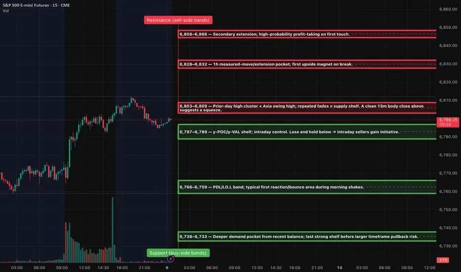
G7 and G20: The Powerhouses Shaping the Global Market LandscapeIntroduction: The Giants Behind the Global Economy
In the modern financial world, two alliances stand out as the nerve centers of global economic governance — the G7 (Group of Seven) and the G20 (Group of Twenty). These powerful coalitions bring together the world’s most influential economies to discuss, design, and direct international economic and financial policies. They influence everything from trade and taxation to debt relief and digital innovation.
While the G7 represents the established industrialized powers, the G20 bridges the developed and developing worlds, making it the most comprehensive global economic forum. Together, they shape policies that impact every corner of the world — from Wall Street to rural villages in emerging economies. Understanding how these groups operate offers a lens into the mechanics of the global market, power politics, and economic diplomacy.
1. The Birth of Economic Alliances
1.1 Origins of the G7
The G7 was born out of a crisis. In the early 1970s, the world was shaken by the collapse of the Bretton Woods fixed exchange rate system and the 1973 oil shock. To restore order and coordinate responses, finance ministers from the U.S., U.K., France, Germany, Japan, and Italy met in 1975. Canada joined soon after, forming the Group of Seven.
Their goal was clear — to stabilize global finance and prevent future crises through collective decision-making. Over time, the G7 expanded its focus to include issues like climate change, development, and technological innovation.
1.2 The Rise of the G20
The G20 emerged in 1999 after the Asian Financial Crisis, which exposed the limits of the G7’s reach. The global economy had changed — emerging markets like China, India, and Brazil were becoming major players. It was no longer sustainable for a handful of rich nations to dictate global economic policy.
The G20 was created to include both advanced and emerging economies, representing about 85% of global GDP, 75% of global trade, and two-thirds of the world’s population. It became the main platform for managing international economic cooperation, especially after the 2008 Global Financial Crisis.
2. Composition and Membership: Power in Numbers
2.1 G7 Members
United States
United Kingdom
Canada
France
Germany
Italy
Japan
The European Union also participates as a non-enumerated member.
These countries share democratic values, high income levels, and deep-rooted industrial and financial systems. Their combined GDP accounts for nearly 45% of global wealth, giving them substantial leverage over world financial markets.
2.2 G20 Members
The G20 includes all G7 members plus:
Argentina, Australia, Brazil, China, India, Indonesia, Mexico, Russia, Saudi Arabia, South Africa, South Korea, and Turkey.
It also includes the European Union as a bloc and invites key international organizations such as the IMF, World Bank, WTO, and OECD.
This blend of developed and developing nations makes the G20 a unique platform — it balances the perspectives of the industrialized North and the fast-growing South.
3. The G7’s Role in the Global Market
The G7 is often viewed as the “executive club” of the world’s most advanced economies. Though small in size, its impact is vast.
3.1 Setting the Economic Agenda
The G7 influences monetary and fiscal policies globally. Decisions made in G7 summits can shape currency values, interest rate expectations, and global trade policies.
For example:
1985 Plaza Accord — The G7 agreed to weaken the U.S. dollar to fix global trade imbalances.
2017–2022 Discussions — Focused on countering protectionism and strengthening global supply chains after trade wars and the COVID-19 pandemic.
3.2 Defending the Rules-Based Order
The G7 champions free markets, democracy, and transparency. It sets global standards for corporate governance, anti-corruption measures, and digital taxation. These principles ensure fairer competition in international trade.
3.3 Crisis Management and Sanctions
The G7 often acts as the “first responder” to global crises. Whether it’s debt relief for Africa in the 2000s or coordinated sanctions against Russia after the 2022 Ukraine invasion, the G7 uses economic tools to enforce geopolitical stability.
4. The G20’s Global Reach and Impact
The G20’s strength lies in its diversity and representation. It brings emerging powers into conversations once dominated by Western nations.
4.1 Post-2008 Financial Stability
The 2008 Global Financial Crisis was the G20’s defining moment.
When major economies were collapsing, the G20 coordinated massive fiscal stimulus packages worth trillions of dollars, stabilized banking systems, and reformed global financial regulations.
It was under G20 leadership that institutions like the Financial Stability Board (FSB) were strengthened to monitor systemic risks.
4.2 Promoting Sustainable Development
The G20 drives discussions on climate financing, green energy transitions, and digital inclusion.
Initiatives such as the G20 Compact with Africa and Sustainable Finance Working Group aim to ensure equitable growth across continents.
4.3 Bridging Inequality
Unlike the G7, the G20 focuses on reducing the global wealth gap.
By including countries like India, Brazil, Indonesia, and South Africa, it gives a voice to nations representing billions of people who were historically excluded from global economic governance.
5. G7 vs. G20: Cooperation or Competition?
While both groups aim for global stability, their roles and structures differ significantly:
Aspect G7 G20
Founded 1975 1999
Members 7 advanced economies 19 nations + EU
Focus Policy coordination among rich nations Global economic cooperation including emerging markets
GDP Share ~45% of global GDP ~85% of global GDP
Decision-Making Consensus-driven, smaller group Broader participation, slower decision-making
Representation Western-oriented Inclusive of Global South
Both groups, however, often coordinate behind the scenes. For instance, during the 2008 crisis, G7 finance ministers first met to frame the response, which was then expanded and executed through the G20.
This “division of labor” ensures speed, inclusiveness, and global legitimacy.
6. Influence on Global Markets and Trade
6.1 Currency and Monetary Policy
The G7 plays a key role in coordinating exchange rates and interest policies among major central banks (like the Fed, ECB, and BoJ).
Even subtle policy shifts discussed in G7 meetings can cause large movements in Forex markets and bond yields.
The G20, meanwhile, focuses on preventing “currency wars” — competitive devaluations that disrupt global trade balance.
6.2 Trade and Supply Chains
Both G7 and G20 promote free trade, but with modern twists.
Recent discussions revolve around “de-risking” supply chains from geopolitical tensions, especially between China and the West.
The G20 supports diversifying global manufacturing to countries like India, Vietnam, and Indonesia — reshaping global trade maps.
6.3 Energy and Climate
Energy security is now central to both groups.
The G7 is pushing for net-zero emissions by 2050, while the G20’s broader approach accommodates developing nations’ need for affordable energy transitions.
This balance affects global oil prices, carbon markets, and renewable energy investments.
7. Challenges Facing G7 and G20
7.1 Geopolitical Tensions
Disagreements over Russia’s invasion of Ukraine, the Israel–Gaza conflict, and the U.S.-China rivalry have often divided members.
The G20’s 2023 New Delhi Summit, for example, struggled to achieve consensus on language condemning wars — showing the complexity of managing global politics through economic platforms.
7.2 Economic Fragmentation
The rise of protectionism, trade barriers, and regional blocs (like BRICS) threatens the unity and influence of G7 and G20.
Emerging powers demand more representation and equitable policy decisions.
7.3 Climate and Digital Divide
While advanced economies focus on decarbonization, developing members emphasize growth and employment.
Bridging this gap — especially in AI, digital finance, and sustainability — will determine the future credibility of both groups.
8. The Future of Global Economic Governance
8.1 The G20 as the New Economic Parliament
With the global economy becoming multipolar, the G20 is expected to play a parliamentary role in global economic governance. It can balance Western dominance with Asian, African, and Latin American representation.
8.2 The G7’s Continued Relevance
Despite its smaller size, the G7 remains powerful due to its financial institutions, innovation leadership, and military alliances. Its policy influence, particularly through the IMF, World Bank, and WTO, continues to define market trends.
8.3 Synergy for Stability
Going forward, global challenges — from inflation to digital currency regulation — will require coordinated action. The ideal future would see the G7’s precision and resources combined with the G20’s inclusiveness and legitimacy.
9. G7 and G20 in the Indian Context
India’s growing global influence has made it a bridge nation between developed and developing worlds.
As G20 President in 2023, India emphasized digital inclusion, sustainable development, and debt relief for the Global South.
The creation of the India–Middle East–Europe Economic Corridor (IMEC) during the G20 Summit redefined strategic trade routes.
India’s balanced diplomacy between the West and BRICS has strengthened its position as a key player in shaping future global governance.
Conclusion: Steering the Global Market’s Destiny
The G7 and G20 together form the twin engines of the global economy.
The G7 provides the financial muscle and institutional leadership, while the G20 ensures diversity, representation, and inclusiveness.
In an era marked by economic volatility, climate urgency, and technological disruption, their coordination is more crucial than ever.
From setting global interest rates to shaping sustainable development goals, these groups influence every major decision that drives the global market.
The world’s economic future — whether stable or turbulent — will depend largely on how effectively the G7 and G20 collaborate to balance growth with equity, power with responsibility, and innovation with sustainability.

How Shipping, Freight, and Logistics Power Global Market Trading🌍 Introduction: The Invisible Engine Behind Global Trade
Every product that moves across borders — from a smartphone in New York to coffee beans in Paris — owes its journey to the vast and intricate world of shipping, freight, and logistics. These three elements form the invisible yet powerful engine that keeps the global market trading ecosystem running.
Behind every trade agreement, export figure, and import bill, lies a network of ships, trucks, planes, and warehouses. Without this system, the flow of goods would come to a standstill, crippling international economies. As globalization deepens, logistics isn’t just about moving products — it’s about synchronizing global supply chains, optimizing cost efficiency, and maintaining the balance of trade across continents.
In today’s dynamic market, logistics has evolved into a strategic weapon. Countries with superior shipping infrastructure and efficient freight management command a strong position in global trade. Let’s explore how these sectors intertwine to shape the global market’s future.
⚙️ 1. Understanding the Triad: Shipping, Freight, and Logistics
Before diving deeper, it’s essential to distinguish between these three interconnected terms:
Shipping: Refers to the actual physical transportation of goods from one location to another — typically over sea or air.
Freight: Represents the cargo itself or the cost of transporting it. Freight can move via air, land, or sea.
Logistics: A broader term encompassing the entire process — from procurement and storage to shipment, tracking, and delivery.
Together, they form a supply chain ecosystem that connects producers, suppliers, distributors, and consumers across continents.
🚢 2. The Backbone of Global Trade: Maritime Shipping
The shipping industry handles over 80% of global trade by volume. Massive container ships, each capable of carrying over 20,000 TEUs (Twenty-foot Equivalent Units), connect major trade hubs like Shanghai, Rotterdam, Dubai, and Los Angeles.
Why Shipping Dominates:
Cost Efficiency: Sea transport remains the most economical for bulk goods.
Scalability: Ships can carry massive loads, making them ideal for global trade.
Connectivity: Ports link multiple continents through trade routes like the Suez Canal, Panama Canal, and the Strait of Malacca.
Key Global Shipping Hubs:
Singapore: Known for its ultra-modern port infrastructure and strategic location.
China (Shanghai & Ningbo): The heart of global manufacturing and export.
Rotterdam (Netherlands): Europe’s largest port and logistics gateway.
Dubai (Jebel Ali): The Middle East’s most significant trade link.
Challenges in Modern Shipping:
Port Congestion: Especially during global disruptions like COVID-19.
Rising Fuel Costs: Impacting freight rates worldwide.
Environmental Regulations: The shift toward green shipping (LNG, electric, hydrogen-powered vessels).
✈️ 3. Freight Networks: The Arteries of the Global Market
Freight is the lifeblood of commerce. It moves raw materials to factories, finished products to retailers, and food to consumers. The freight sector spans multiple modes:
a) Sea Freight
Still the most widely used due to lower costs. However, it’s slower, making it less suitable for time-sensitive cargo.
b) Air Freight
Used for high-value, urgent, or perishable goods — electronics, pharmaceuticals, and luxury items.
Example: A smartphone assembled in China reaches the U.S. in under 48 hours via air freight.
c) Land Freight (Trucking & Rail)
Essential for last-mile connectivity and regional trade.
Rail Freight: Gaining importance through transcontinental networks like China-Europe Railway Express.
Truck Freight: Vital for connecting ports, airports, and inland destinations.
Freight Pricing Dynamics
Freight rates are influenced by:
Fuel prices (bunker fuel, aviation fuel)
Port handling charges
Supply-demand imbalances
Geopolitical tensions (e.g., Red Sea or Black Sea blockages)
Global crises (pandemics, wars, etc.)
For instance, during the 2021–22 period, container freight rates between Asia and the U.S. soared by over 300%, revealing how fragile and demand-sensitive freight economics are.
🏗️ 4. Logistics: The Brain of the Operation
If shipping is the muscle and freight is the blood, logistics is the brain coordinating every movement.
Modern logistics involves:
Supply chain planning
Inventory management
Warehousing and distribution
Real-time tracking systems
Customs and documentation handling
The Digital Transformation of Logistics
The logistics industry is undergoing a technological revolution:
IoT sensors track container temperature and location.
AI algorithms optimize routes and predict disruptions.
Blockchain ensures transparency and authenticity in transactions.
Drones and robotics accelerate warehouse operations.
Major Global Logistics Players
DHL (Germany) – Known for integrated logistics and global air freight.
Maersk Logistics (Denmark) – Evolved from a shipping company to an end-to-end logistics leader.
FedEx and UPS (USA) – Masters of express logistics.
DB Schenker, Kuehne + Nagel – Giants in multimodal transport and supply chain management.
📈 5. How Logistics Shapes Global Market Trading
The performance of logistics directly impacts global market trading trends, particularly in:
a) Trade Competitiveness
Efficient logistics reduce costs and delivery time, giving countries an edge.
For example, Vietnam and Bangladesh have become major textile exporters due to improving port and logistics infrastructure.
b) Stock Market Sensitivity
Shipping and logistics stocks often act as economic barometers.
When freight demand rises, it signals stronger global trade — often boosting related equities like Maersk, Cosco, or FedEx.
c) Commodity Flow and Pricing
Delays or disruptions in shipping (like the 2021 Suez Canal blockage) can skyrocket oil and commodity prices, shaking markets worldwide.
d) Currency and Inflation Effects
Rising freight costs translate into import inflation, affecting consumer prices and currency values.
🌐 6. The Emerging Trends Transforming the Industry
The next decade of shipping and logistics will be defined by technology, sustainability, and geopolitical realignment.
a) Green Shipping Revolution
To meet carbon-neutral goals, companies are investing in:
Biofuel and hydrogen vessels
Electric trucks and hybrid cargo ships
Port electrification and automation
b) Digital Freight Platforms
Startups and major logistics firms are digitizing operations. Platforms like Flexport, Freightos, and Maersk Spot allow real-time booking, rate comparison, and shipment tracking.
c) Regionalization of Supply Chains
The pandemic taught companies not to depend on single regions (like China). “China +1” strategies are leading to diversification into India, Vietnam, and Mexico.
d) Autonomous Transport
Self-driving trucks are being tested for long-haul logistics.
AI-powered ships are navigating test routes autonomously.
e) Cold Chain Expansion
As pharmaceutical and perishable goods trading grows, demand for temperature-controlled logistics (cold chain) is booming globally.
💥 7. Challenges Facing the Global Shipping and Logistics Sector
Despite its importance, the industry faces intense challenges:
Geopolitical Tensions: Trade wars and conflicts disrupt established routes (e.g., Russia-Ukraine, Red Sea tensions).
Fuel and Energy Volatility: Shipping heavily depends on bunker fuel; any spike raises freight costs globally.
Environmental Regulations: IMO 2020 sulfur caps and net-zero emission goals are increasing operational costs.
Port Infrastructure Gaps: Developing nations face bottlenecks due to outdated facilities.
Digital Divide: Smaller logistics players struggle to adopt advanced tech systems.
Labor Shortages: Shortage of truck drivers, dock workers, and technical staff affects global efficiency.
🧭 8. Future Outlook: The Next Wave of Global Logistics
By 2030, the logistics landscape will look very different:
Smart Ports: Automated cranes, AI scheduling, and blockchain customs.
Hyperloop & Drone Delivery: Faster, cleaner alternatives for intercity and last-mile logistics.
Decentralized Trade Routes: Africa and South America emerging as new freight corridors.
Resilient Supply Chains: Diversification and AI forecasting will reduce dependency on any single geography.
The integration of AI and blockchain will bring transparency and traceability to global supply chains, reducing fraud and inefficiencies. Meanwhile, green logistics will become a major investment theme, attracting ESG-focused capital.
💡 9. Investment & Trading Opportunities in the Sector
For traders and investors, shipping and logistics offer exciting opportunities:
Publicly Listed Giants: Maersk, Hapag-Lloyd, Evergreen Marine, FedEx, and UPS often move in sync with trade growth cycles.
Port Operators: DP World, Adani Ports, and Hutchison are key beneficiaries of rising trade volumes.
Logistics Tech Startups: AI-driven freight management firms are disrupting traditional models.
ETF Exposure: Funds like the Global X Shipping ETF allow investors to ride global logistics growth.
As e-commerce and manufacturing expand globally, logistics stocks could become the backbone of long-term investment portfolios.
🏁 Conclusion: The Flow That Never Stops
Global market trading is like a living organism — and shipping, freight, and logistics are its vital organs. Every container that moves, every parcel delivered, and every port expansion project fuels the heartbeat of the world economy.
As the 21st century progresses, this industry is not just about transportation anymore. It’s about technology, sustainability, and strategy. Those who master logistics control the rhythm of world trade.
From AI-managed ports to zero-emission ships, the next decade promises a revolution in how goods move across the planet — faster, cleaner, and smarter. In the grand theater of global markets, logistics remains the silent powerhouse that keeps the world connected and commerce alive.
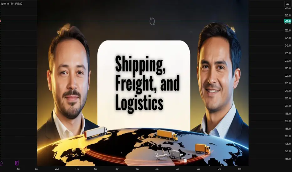
Exchange Rate Secrets1. What Are Exchange Rates and Why They Matter
An exchange rate is simply the price of one currency in terms of another. For instance, if $1 = ₹84, that means one US dollar can buy eighty-four Indian rupees.
But this number isn’t just a conversion figure — it’s a snapshot of economic power.
When a country’s currency strengthens, imports become cheaper but exports turn costlier.
When it weakens, exports surge but inflation might rise.
Exchange rates influence:
Global trade balances
Investment decisions
Inflation and interest rates
Tourism and remittances
Stock and commodity markets
Understanding these hidden levers is the first step to decoding the secrets of exchange rate movements.
2. The Real Players Behind the Curtain
Contrary to popular belief, exchange rates don’t move by chance. They’re often influenced — directly or indirectly — by a select few economic giants:
a. Central Banks
Institutions like the US Federal Reserve, European Central Bank, and Reserve Bank of India hold the real levers.
They manipulate interest rates to attract or repel foreign capital.
They intervene in forex markets to stabilize or deliberately weaken their currency.
They issue monetary policies that send shockwaves through global markets.
For example, when the Fed raises interest rates, the US dollar usually strengthens — because higher returns attract global investors.
b. Institutional Traders and Hedge Funds
Major hedge funds trade billions in currencies daily. They anticipate policy changes and use leverage to amplify profits — creating massive short-term moves that can destabilize weaker economies.
c. Governments
Sometimes, governments quietly “manage” their exchange rates for strategic reasons. China, for example, has often been accused of keeping the Yuan undervalued to make its exports more competitive — a tactic dubbed “currency manipulation.”
d. The Market Psychology
Beyond data and policy, market sentiment — the collective emotion of traders — drives currencies. Fear of recession, geopolitical tensions, or even rumors can send exchange rates spinning faster than any spreadsheet can predict.
3. The Core Secrets Behind Currency Movements
Now let’s unlock the deep, often hidden mechanisms that move currencies. These are the five pillars of exchange rate secrets:
1️⃣ Interest Rate Differentials
Currencies tend to flow toward countries with higher interest rates.
If India’s rates are 6% while the US offers 4%, investors may convert dollars to rupees to earn better returns.
This inflow strengthens the rupee.
But here’s the twist: expectations matter more than reality. Even a hint that the Fed may raise rates can trigger massive dollar inflows — long before the actual hike happens.
2️⃣ Inflation and Purchasing Power
Currencies are mirrors of purchasing power.
If inflation is high in one country, its money loses value faster.
Low inflation, on the other hand, indicates stability and boosts confidence.
This is why nations with consistent inflation control — like Switzerland and Japan — often see their currencies appreciated as “safe havens.”
3️⃣ Trade Balances
Countries that export more than they import tend to have stronger currencies.
Why? Because foreign buyers must purchase the exporter’s currency to pay for goods.
For instance, Japan’s trade surplus has historically supported the yen.
Conversely, a nation running persistent trade deficits (like the US) faces downward pressure — unless offset by investment inflows.
4️⃣ Political Stability and Global Confidence
Political chaos often sends investors fleeing.
A coup, election turmoil, or policy uncertainty can cause sudden devaluations.
Meanwhile, stable governments with clear fiscal policies attract long-term investors — strengthening the currency.
When Russia invaded Ukraine in 2022, the ruble initially collapsed. Yet, with aggressive capital controls and energy exports, it later stabilized — showcasing how government measures can rewrite currency fate.
5️⃣ Speculation and Market Manipulation
The most guarded secret: exchange rates aren’t always fair reflections of fundamentals.
Short-term volatility is often fueled by speculation — big money betting on future trends.
Speculators can move billions in seconds, pushing prices away from equilibrium.
Sometimes, their combined power even forces central banks to retreat — like in 1992’s “Black Wednesday”, when George Soros famously broke the Bank of England and earned over $1 billion in a single day.
4. The Hidden Mechanisms: Pegs, Floats, and Hybrids
Every country chooses how “free” its exchange rate should be.
A. Fixed (Pegged) Exchange Rate
Here, the value is tied to another currency, like the US dollar.
Example: Saudi Arabia pegs its riyal to the dollar to stabilize oil revenues.
Advantage: predictability for trade.
Disadvantage: vulnerability to external shocks.
B. Floating Exchange Rate
The value fluctuates based on market demand and supply.
Example: The US dollar, euro, and Indian rupee are managed floats.
Advantage: market-driven flexibility.
Disadvantage: volatility during crises.
C. Managed Float (Dirty Float)
Most modern economies use this hybrid system — allowing markets to move rates but stepping in occasionally to maintain stability.
These systems reveal another secret — that exchange rates are both economic tools and political weapons.
5. Currency Wars and Global Power Play
When one country weakens its currency intentionally, others often retaliate — sparking a currency war.
The logic is simple: a cheaper currency boosts exports and jobs.
But when multiple nations do this simultaneously, it can spiral into global instability.
2010s: The US accused China and Japan of undervaluing their currencies.
2020s: Nations quietly use quantitative easing (printing money) to keep currencies weak.
2025: As emerging markets like India, Brazil, and Indonesia grow, they’re joining this silent battle — balancing competitiveness with credibility.
6. The Psychological Side of Exchange Rates
Money is emotional. Exchange rates reflect not just economic numbers, but confidence.
When investors “believe” in a country’s future — its leadership, innovation, and growth — its currency rises.
Example:
The US dollar thrives during crises — seen as a “safe haven.”
The Swiss franc and Japanese yen surge when global uncertainty spikes.
The Indian rupee strengthens when foreign investors see long-term growth potential.
This psychological dance creates cycles — optimism, panic, correction — that drive exchange rate volatility beyond fundamentals.
7. Modern Secrets: Digital Currencies and Forex Algorithms
The 21st century has introduced new players and tools that redefine how currencies behave.
a. Algorithmic Trading
Over 70% of forex volume now runs on algorithms — automated systems that execute trades based on millisecond data.
These algorithms can amplify moves, creating sharp spikes or sudden reversals within seconds.
b. Cryptocurrencies
Bitcoin and stablecoins have disrupted the concept of “sovereign money.”
Some nations fear them; others embrace them.
El Salvador adopted Bitcoin, while China banned it and launched its own digital yuan — a step toward controlling cross-border transactions.
The secret here: digital currencies could one day bypass traditional exchange rates altogether.
8. The Indian Rupee in the Global Context
India’s exchange rate journey is a fascinating case study:
Pre-1991: A fixed regime tied to the pound, later the dollar.
Post-liberalization: A managed float system with RBI intervention.
Today: The rupee reflects both domestic fundamentals and global capital flows.
Hidden truth?
The RBI quietly smoothens volatility through buying or selling dollars — maintaining competitiveness for exports while protecting inflation targets.
Future outlook:
Stronger digital economy
Growing exports (IT, pharma, energy)
Controlled fiscal deficit
All point toward a more resilient rupee in the long run — though short-term fluctuations will remain.
9. How Traders and Investors Decode Exchange Rate Secrets
Smart investors don’t just watch the numbers — they watch the forces behind them.
Here’s how they stay ahead:
Monitor central bank statements — “forward guidance” often signals currency direction.
Track bond yield differentials — a widening gap means a stronger high-yield currency.
Follow geopolitical developments — sanctions, wars, or trade deals often move currencies overnight.
Use Volume Profile and Market Structure — to identify institutional footprints in forex charts.
Analyze capital flow data — especially FII (Foreign Institutional Investor) movements in emerging markets like India.
By understanding these undercurrents, traders can align with the smart money — not against it.
10. The Future of Exchange Rates: Toward a Digital Reset
Global monetary systems are entering a new era.
The next decade may witness a “global currency reset”, where traditional paper currencies evolve into central bank digital currencies (CBDCs).
This shift could:
Reduce transaction costs
Increase surveillance and control
Challenge the dominance of the US dollar
Create new “exchange rate ecosystems” driven by technology rather than trade alone
In short, the secrets of tomorrow’s exchange rates may lie not in central banks alone, but in blockchain codes and algorithmic governance.
Conclusion: The Art and Science of Exchange Rates
Exchange rates are far more than numbers flashing on a trading screen.
They are reflections of economic strength, political will, psychological trust, and technological evolution.
The secret to understanding them lies in reading between the lines — connecting data with direction, policies with perception, and numbers with narratives.
As global markets evolve, those who grasp these hidden forces won’t just convert currencies — they’ll convert opportunities into fortune.
Because in the end, exchange rates aren’t just about money — they’re about power. 🌍💰