Adaptive AI SuperTrend [AlgoPoint]🚀 Adaptive AI SuperTrend
Adaptive AI SuperTrend is a high-performance trading terminal that redefines trend-following by integrating Machine Learning (ML) principles with advanced market regime detection. Unlike static indicators, this system dynamically recalibrates its internal parameters to match the ever-changing volatility of the financial markets.
Equipped with a custom "Wizard Engine," it filters out market noise during consolidation and identifies high-probability trend continuation points, making it an essential tool for scalpers, day traders, and swing traders alike.
🧠 What Makes it "AI"?
While traditional indicators use fixed rules, Adaptive AI SuperTrend utilizes Algorithmic Intelligence to make real-time decisions:
KNN-Inspired Adaptation: The engine analyzes the last 150 bars of volatility and trend strength to automatically adjust its sensitivity.
Market Regime Intelligence: It distinguishes between "Trending" and "Ranging" states using a sophisticated Squeeze Momentum module, preventing "whipsaws" during low-volume periods.
Self-Backtesting Logic: The indicator continuously calculates its own historical Win-Rate. If the probability of success falls below a certain threshold, it suppresses lower-quality signals.
🛠 Key Features
Dynamic Consolidation Boxes: Automatically identifies and wraps "choppy" price action in professional gray boxes. It waits for 3+ bars of consolidation before marking the zone, helping you spot breakout opportunities early.
Multi-Strategy Aggression:
- Conservative: Filtered signals for long-term trend following.
- Balanced: Optimized for daily volatility.
- Aggressive: High-frequency signals for capturing micro-trends.
Dual-Exit Risk Management:
- ATR TP-SL Mode: Sets mathematical targets based on market volatility with persistent on-screen lines.
- Smart Trailing Mode: Rides the trend to its exhaustion point. Includes intelligent labeling (🎯 TP or 🛑 SL) based on the trade's net profitability.
- RSI Pullback Confirmation: Beyond simple trend flips, it detects "buy the dip" or "sell the rip" opportunities within an existing trend using RSI 50-level crossovers.
📊 Real-Time Analytics Dashboard
The integrated AlgoPoint Dashboard provides a surgical view of the market:
- Market State: Instant "Trending" vs. "Ranging" (Consolidation) detection.
- Trend Strength: ADX-based momentum tracking.
- Strategy Status: Real-time feedback on your active aggression and exit modes.
🎨 Clean Charting & Customization
Built for professional clarity, you have total control over the UI:
Toggle Consolidation Boxes on/off.
Toggle ATR Target Lines and Exit Labels.
Customize background filters and dashboard visibility.
AI

AI Trend Targets Oscillator- Webhooks v1.8.1AI Trend Targets Oscillator - Webhooks v1.8.1
www.cryptogenix.club
General Description
AI Trend Targets Oscillator is an advanced trading indicator that combines the power of artificial intelligence with technical analysis to provide precise trading signals and automatically optimized Take Profit (TP) targets. The indicator uses AI algorithms to learn from past performances and adapt Take Profit levels based on the specific behavior of the market you're trading.
🎯 Main Features
1. Intelligent Trading Signals (BUY/SELL)
The indicator generates clear buy and sell signals based on a sophisticated oscillator that analyzes:
• Market momentum - quickly identifies trend changes
• Overbought/oversold zones - filters out false signals
How it works:
• BUY (Long) signals appear when the indicator detects optimal conditions for entering a long position
• SELL (Short) signals appear when conditions are favorable for short positions
• Each signal comes with visual markers both in the indicator pane and on the price chart
2. AI Take Profit Optimization System
This is the KEY function that differentiates this indicator!
Unlike traditional indicators that use fixed TP levels, this indicator uses Artificial Intelligence to automatically calculate the most likely profit targets based on:
How the AI works:
• Analyzes the last N trades (configurable, default 20) for each direction (BUY/SELL separately)
• Measures Maximum Favorable Excursion (MFE) - how far the price moved in your favor in each previous trade
• Calculates statistical percentiles to determine TP levels with high success probability
Three Intelligent Take Profit Levels:
TP1 (Conservative):
• Default target: 66% success rate
• The closest objective, for quickly securing part of the profit
• Ideal for defensive strategies or volatile markets
TP2 (Moderate):
• Default target: 50% success rate
• Balance between safety and profit
• Recommended level for most traders
TP3 (Aggressive):
• Default target: 30% success rate
• Ambitious target for profit maximization
• For traders with higher risk tolerance
Important: These success percentages are CONFIGURABLE - you can adjust each level based on your trading style!
Advanced AI Features:
• Adaptive learning - The more you trade, the more accurate the AI becomes for your specific pair
• Direction separation - The AI learns separately for LONG and SHORT positions (the market behaves differently in uptrend vs downtrend)
• Dynamic updates - TP levels are automatically recalculated as new trades are added to history
3. Dynamic and Intelligent Stop Loss
The Stop Loss system is designed for maximum protection:
How it's calculated:
• Uses the Donchian Channel method to identify recent lows/highs
• Adds an ATR (Average True Range) buffer to avoid premature stops caused by normal volatility
• Fully configurable - you can adjust both the Donchian period and the ATR multiplier
Advantages:
• Automatically adapts to market volatility
• Avoids "shakeouts" - stops hit by normal fluctuations
• Provides optimal asymmetric protection (low risk, high profit)
4. Real-Time Statistics Table
The statistics panel is ESSENTIAL for performance evaluation and settings optimization!
What it displays:
For the last N trades (separately for BUY and SELL):
• Wins - number of winning trades (that reached SL or a TP in profit)
• Loss - number of losing trades
• TP1 Hit % - percentage of trades that reached the first take profit
• TP1 Pending % - percentage of trades that are still active or haven't reached TP1
• TP2 Hit % and TP2 Pending % - statistics for the second take profit
• TP3 Hit % and TP3 Pending % - statistics for the third take profit
Automatic Recommendation System:
The indicator automatically analyzes performance and provides three types of feedback:
🛑 "We do NOT recommend trading this pair"
• Appears when both LONG and SHORT positions have over 40% losses
• Signal that settings or the pair are not optimal
• Tip: Try another pair or adjust parameters
⚠️ "Trading is risky with these settings"
• One of the directions (LONG or SHORT) has poor performance
• You can selectively trade only the profitable direction
• Tip: Refine general settings or trade only the good direction
✅ "You can trade this pair"
• Both directions (LONG and SHORT) have under 40% losses
• Green signal for active trading
• Confirmation that settings are well calibrated for this pair
Importance: This system automatically protects you from trading on markets unsuitable for your strategy!
YOU WILL RECEIVE PRICE ALERTS ON A COIN ONLY IF THE STATUS IS ✅ "You can trade this pair"
5. Historical TP and SL Overlays
For each past signal, you can visualize:
On the price chart:
• Entry line (yellow) - the price at which the signal was generated
• Stop Loss line (red) - protection level
• TP1, TP2, TP3 zones (green/red gradual) - all three profit targets
• Status markers:
o ⊙ = TP successfully reached (green)
o ◯ = TP not yet reached (gray)
Utility:
• Visual evaluation of performance across all trades
• Identification of success/failure patterns
• Quick verification if AI levels are realistic for the market
8. Webhook Integration for Automated Trading
The indicator is ready for complete automation:
Combined alert:
• Triggers ONLY when the signal is valid (footer with ✅)
• Triggers ONLY at bar close (not mid-bar)
• Includes all necessary information: symbol, timeframe, direction
Compatible with:
• Automated trading platforms (3Commas, Cornix, etc.)
• Custom bots
• Notification systems (Telegram, Discord, Email)
📊 How to Use the Indicator
Recommended Workflow:
1. Initial Setup:
o Add the indicator to the chart
o Leave default settings for beginning
o Observe the statistics table
2. Learning Period (20+ bars):
o Allow the indicator to collect data
o Check the footer for status message
o DO NOT trade until you have ✅ in footer
3. Optimization:
o Analyze statistics from the table
o If Loss % > 40% for both directions → adjust parameters
o If only one direction is profitable → trade selectively
o Adjust Target Success % for TPs based on market
4. Active Trading:
o Follow only signals with footer ✅
o Enter on confirmed BUY/SELL signal
o Place SL at shown level
o Place all 3 TPs (or just those that suit you)
o Monitor table for continuous adjustments
Usage Strategies:
Conservative:
• Use only TP1 and TP2
• Larger SL Buffer (1.5-2.0 ATR)
• Higher Target Success % (80/60/40)
• Trade only when both directions are ✅
Moderate:
• Use all 3 TPs
• Default settings
• Trade selectively based on footer
Aggressive:
• Focus on TP3 for large profits
• Lower Target Success % (50/30/15)
• Smaller SL Buffer (0.5-1.0 ATR)
• Accept higher risk for higher reward
🎓 Indicator Strengths
✅ Complete adaptability - Automatically adjusts to any financial instrument ✅ Continuous learning - With each trade, it becomes more accurate ✅ Built-in protection - Automatic evaluation system prevents trading on unsuitable markets ✅ Total transparency - See all statistics and performance in real-time ✅ Maximum flexibility - All important aspects are customizable ✅ Complete risk management - TP and SL calculated automatically for each trade ✅ Zero lag in signals - Bar close confirmation eliminates repainting ✅ Automation ready - Webhooks for bot integration
⚠️ Important Recommendations
1. DO NOT ignore the footer - If you don't have ✅, don't trade!
2. Respect the SL - It's mathematically calculated for optimal protection
3. Allow learning - Minimum 20-30 trades for precise AI calibration
4. Monitor statistics - The table tells you when to adjust settings
5. Test first - Use paper trading or demo to understand the indicator
6. Don't mix strategies - If you use AI for TP, don't manually modify them frequently
🔧 Who Is This Indicator For?
Perfect for:
• Traders who want automatic TP/SL optimization
• Those who trade multiple pairs and want consistency
• Automated trading through bots/webhooks
• Swing traders and day traders
• Traders who want instant performance feedback
Less suitable for:
• Ultra-fast scalping (< 1 minute)
• Those who prefer 100% manual analysis
• Traders who don't follow risk management rules
📈 Recommended Timeframes
The indicator works on any timeframe but is optimized for:
• 15 minutes - Active day trading
• 1 hour - Short-term swing trading
• 4 hours - Medium swing trading
• Daily - Position trading
Note: The higher the timeframe, the fewer but more reliable the signals!
💡 Pro Tip
Combine this indicator with:
• Volume analysis for confirmations
• Major support/resistance zones
• Candle patterns for fine timing
• Multiple timeframes for confluence
Don't forget: The AI learns from ALL trades, including losing ones! Each trade makes it smarter!
Disclaimer: This indicator is a technical analysis tool. It does not guarantee profits and does not constitute financial advice. Trade responsibly and manage your risk correctly!

Mission Control Dashboard (AI, Crypto, Liquidity) FASTCONCEPT Price is a lagging indicator. Liquidity is a leading indicator. "Mission Control Dashboard (AI, Crypto, Liquidity) FAST" is a sophisticated macroeconomic dashboard designed to audit the "plumbing" of the financial system in real-time. Unlike standard indicators that rely solely on price action, this tool pulls data from the Federal Reserve (FRED), Treasury Statements, Corporate Financials (10-K/10-Q), and On-Chain Stablecoin metrics to visualize the structural flows driving the market.
THE "UNIFIED FIELD" SOLVER One of the hardest challenges in cross-asset scripting is "Time Dilation"—synchronizing 24/7 Crypto markets (Bitcoin) with Mon-Fri Traditional markets (Stocks/Bonds).
Standard scripts fail on weekends, showing mismatched data.
This engine uses a Weekly Anchor system. It calculates all momentum and liquidity metrics based on "Week-to-Date" or "Month-Ago" anchors. This ensures that a "Liquidity Drain" looks identical whether you are viewing a Bitcoin chart on Saturday or an Apple chart on Monday.
THE CHRONOS LOGIC The dashboard is sorted by Time Sensitivity (Speed of impact), from fast-twitch tactical signals to slow-moving structural fundamentals.
1. TACTICAL (Reacts in 24–48h)
Stablecoin Flight: Measures the immediate flow of capital from Volatile Assets to Stablecoins (USDT/USDC). A spike (>0.5%) indicates fear/sidelining.
Liquidity Alpha: Calculates the efficiency of capital. It subtracts "Friction" (Dollar Strength + Yields) from "Flow" (Liquidity Beta). High Alpha means money is flowing easily into risk assets.
Alt Euphoria: Tracks the overheating of the Altcoin market (TOTAL3). Green indicates sustainable growth; Red (>45%) warns of a "blow-off top."
Retail FOMO: A sentiment gauge comparing Coinbase Stock ( NASDAQ:COIN ) performance vs. Bitcoin ( CRYPTOCAP:BTC ). When Retail outperforms the Asset, local tops often follow.
2. LIQUIDITY & MACRO (Reacts in 1–4 Weeks)
Debt Wall (10Y): The Rate-of-Change of the US 10-Year Treasury Yield. Spiking yields act as gravity on risk assets.
Liquidity Beta: The raw "Quantity of Money." Tracks the 4-week change in Net Liquidity (Fed Balance Sheet - TGA + Stablecoins).
TGA Balance: The Critical Monitor. Tracks the Treasury General Account. When the TGA rises (Red), the government is draining liquidity from the banking system. When it falls (Green), it releases cash.
Note: This script includes an auto-scaler to handle TGA data in both Billions and Millions.
3. STRUCTURAL (Reacts in 3–12 Months)
AI Capex (YoY & QoQ): The "Floor" of the 2025/2026 cycle. Tracks the Capital Expenditure of the Hyperscalers (MSFT, GOOGL, AMZN, META). As long as this remains high (>30%), the infrastructure boom supports the tech narrative.
PMI Manufacturing: Tracks the ISM Manufacturing cycle. Contraction (<50) often forces Fed intervention.
Micron Inventory: A lead indicator for the hardware cycle.
HOW TO USE
Status Colors: The traffic light system helps you assess risk at a glance.
🟢 GREEN (Healthy): Flow is positive, friction is low, fundamentals are strong.
🔴 RED (Danger): Liquidity is draining (TGA spike), yields are shock-rising, or FOMO is excessive.
Zero Configuration: The script auto-detects asset classes and scales units (Billions/Trillions) automatically.
DATA SOURCES
Federal Reserve Economic Data (FRED)
Daily Treasury Statement (DTS)
CryptoCap (TradingView)
Nasdaq/Corporate Financials
Disclaimer: This tool is for informational purposes only and does not constitute financial advice. Macro data feeds are subject to reporting delays.

Mission Control Dashboard (AI, Crypto, Liquidity)Description: Mission Control Dashboard (AI, Liquidity) is a comprehensive macro-liquidity and cycle-analysis dashboard designed to track the "Flow of Funds" across traditional and crypto markets. Instead of looking at price action alone, this script monitors the fundamental "plumbing" of the global economy.
Key Metrics Tracked:
The Debt Wall: Monitors the US 10Y Yield and TLT price. It signals a "Critical" state if yields spike above 5% or TLT drops below $80, indicating high stress in the bond market.
Global Liquidity (MTF Stable): A proprietary calculation summing the balance sheets of the FED, ECB, BoJ, and PBoC, plus Stablecoin market cap. It calculates the Rate of Change (ROC) to see if the world is "printing" or "draining" money.
TGA Hidden Fuel: Tracks the Treasury General Account. A falling TGA is often bullish for risk assets as it injects liquidity into the banking system.
Universal Alt Season: Monitors TOTAL3 (Crypto market cap excluding BTC & ETH) for parabolic moves (>30% ROC).
AI Infra Capex: Real-time tracking of Capital Expenditures from MSFT, GOOG, AMZN, and META to gauge the health of the AI cycle.
How to use:
Green Status across the board: High probability for "Risk-On" environments (Alt season, Tech rallies).
Strategic Beta vs. Tactical Alpha: If Beta is draining but Alpha is accelerating, it suggests a "False Breakout" or a divergence in liquidity.
Uranium Trend: Used as a proxy for the energy transition and long-term industrial cycle strength.

Lune Institutional Analysis Premium⬛️ Overview
Lune Institutional Analysis is a comprehensive suite of institutional-grade tools designed to visualize market liquidity and volume dynamics. By utilizing volume clustering and delta analysis, this indicator provides traders with a professional perspective on market activity, highlighting areas where significant volume concentrations occur. It is designed to complement strategies such as SMC (Smart Money Concepts) and ICT (Inner Circle Trader) by providing a data-driven layer of institutional context.
Distinguished by its real-time, non-repainting calculations, Lune Institutional Analysis aims to bridge the gap between retail price action and volume-based institutional data, helping traders identify potential "smart money" footprints.
🟦 Features
Lune Institutional Analysis equips traders with an array of sophisticated features:
🔹 Liquidity Bubbles: This feature visualizes significant volume spikes and concentrations based on volume delta and point of control (POC) analysis within each candle. It identifies imbalances where buy or sell volume significantly outweighs the other. It supports two modes: Regular Bubbles and Trapped Liquidity Bubbles. Trapped Liquidity Bubbles are designed to identify potential "liquidity traps" where price moves sharply against a high-volume area. The Adaptive Transparency feature dynamically adjusts bubble visibility based on the relative volume significance.
🔹 Liquidity Waves: Liquidity Waves track market movements through advanced volume spread analysis, showing the ebb and flow of market interest. By analyzing volume delta patterns, this tool helps traders visualize the momentum of liquidity as it enters or exits the market. It includes sensitivity controls and adaptive transparency to highlight the most significant wave patterns.
🔹 Accumulation/Distribution: The Accumulation/Distribution tool automatically detects and highlights professional accumulation and distribution zones. These zones identify where institutional players are likely building or offloading positions, providing crucial context for potential trend reversals or continuations.
🔹 AI Volume Candles: This feature reimagines price action by integrating volume delta directly into candle visualization. It includes Volume Delta Zones and Net Volume Lines to pinpoint where the most significant trading activity is occurring within each bar. By highlighting volume concentrations, AI Volume Candles reveal the internal strength or weakness of price moves that standard candles might hide.
🔹 AI Liquidation Levels: This tool identifies potential liquidation zones by analyzing historical volume clusters and price pivots. These levels represent areas where a high volume of orders was previously executed, often serving as magnets for price (draw on liquidity) or significant areas of interest for ICT-style analysis. The indicator uses a normalization algorithm to represent volume concentration through dynamic width and adaptive transparency.
🔹 AI Heat Map: The AI Heat Map provides a historical volume distribution visualization, color-coding zones based on net volume delta or directional bias. This reveals the "memory" of the market and where historical interest remains, allowing traders to see significant support and resistance levels formed by historical volume concentrations.
🔹 AI Volume Profile: This sophisticated butterfly-style profile displays both total volume and buy/sell delta distribution. It automatically identifies AI Key Levels (significant volume nodes) that serve as institutional support and resistance. The profile offers deep insights into where value is being perceived by major market participants.
These features and tools collectively offer a comprehensive solution for traders to understand and navigate the financial markets. It's important to remember that they are designed to assist in making informed trading decisions and should be used as part of a balanced trading strategy.
🟧 Usage
Lune Institutional Analysis's unique feature set can be leveraged both individually and synergistically. It is important to understand each feature and experiment with different configurations to best suit your unique trading needs.
🔸 Example #1: The following example demonstrates how Trapped Liquidity Bubbles and AI Liquidation Levels can be used together to identify potential reversal points.
Trapped Liquidity Bubbles highlight areas where market participants may be positioned against a sharp move, while AI Liquidation Levels show historical volume clusters where those positions might face pressure. When a bearish Trapped Liquidity Bubble appears near an AI Liquidation level, it can serve as a confluence signal for a potential price reaction.
🔸 Example #2: This example shows how the AI Volume Profile and AI Heat Map can be used to identify areas of significant interest and volume exhaustion.
The AI Volume Profile's key levels represent nodes of high historical volume. When price approaches an AI Heat Map zone that aligns with a high-volume node, it provides a stronger confirmation of a potential support or resistance area. Observing price reaction at these combined levels can help traders gauge whether a trend is likely to continue or exhaust.
🔸 Example #3: This example demonstrates how AI Volume Candles can be used to confirm trend strength or identify potential absorption.
By using Volume Delta Zones within the AI Volume Candles, traders can see if a breakout is supported by strong directional volume. If price breaks a resistance level but the AI Volume Candles show a high concentration of bearish delta (absorption), it may indicate a fakeout. Conversely, strong bullish delta zones during an uptrend confirm institutional participation in the move.
🟥 Conclusion
Lune Institutional Analysis provides a data-centric bridge between retail analysis and institutional-grade volume data. By offering clear visualizations of liquidity, volume delta, and significant volume clusters, it allows traders to look beyond standard price action and understand the underlying volume dynamics. This suite is built for practitioners of SMC and ICT who require an objective, volume-based confirmation for their setups.
🔻 Access
You can see the Author's instructions below to get instant access to this indicator & our Premium Suite.
🔻 Disclaimer
Lune Institutional Analysis is a tool for aiding in market analysis and is not a guarantee of future market performance or individual trading success. We strongly recommend that users combine our tool with their trading strategies and do their due diligence before making any trading decisions.
Remember, past performance is not indicative of future results. Please trade responsibly.

BLACKBOX AI Trade Sniper [12CROWNS]BLACKBOX AI Trade Sniper
Stop guessing. Start targeting.
The BLACKBOX AI Trade Sniper is an institutional-grade algorithmic trading system designed exclusively for BLACKBOX Trade Journal Pro users. Built for precision scalping and swing trading, this tool eliminates market noise to reveal the true trend.
THE PROBLEM:
Most indicators lag or get chopped up in ranging markets, leading to false signals and drawdown.
THE SOLUTION:
The Trade Sniper synthesizes Renko Brick Construction with Heikin Ashi Smoothing to create a "MagLock" effect. It ignores minor price fluctuations and only fires a signal when a statistically significant structural break is confirmed by volatility (ATR).
---
MISSION CRITICAL FEATURES:
1. Renko-Based Trend Engine (Noise Cancellation)
Instead of reacting to every tick, the AI runs a background simulation using Dynamic Renko Bricks. It auto-adjusts to market volatility using Average True Range (ATR).
- Result: You stay in the trade during chop and only exit when the trend actually reverses.
2. Target Lock Visuals (The Cockpit)
A clean, military-inspired HUD keeps your chart professional and clutter-free.
- Green Target (⌖): Confirmed Bullish Structural Break (Long Entry).
- Red Target (⌖): Confirmed Bearish Structural Break (Short Entry).
- Yellow Warning: Early detection system signaling that price has moved 80% toward a reversal.
3. Volatility "G-Force" Filter
Bad trades happen in low volume. The integrated G-Force monitor analyzes real-time volume vs. baseline averages to filter out weak moves (Crab Market) and highlight high-conviction breakouts.
---
HOW TO USE:
- Scalpers: Use on lower timeframes (1m - 15m) to catch rapid trend shifts with the Renko Engine.
- Swing Traders: Use on higher timeframes (1H - 4H) to filter out intraday noise and ride major moves.
- Risk Management: Utilize the "Sniper Warning" (Yellow Target) to tighten stop-losses before a trend flip occurs.
ACCESS:
This is a proprietary Invite-Only Script protected by 12CROWNS. Access is restricted to active members of the BLACKBOX Trade Journal ecosystem.
For access details and documentation:
12crowns.com
Note: This tool does not repaint. All signals are confirmed upon candle close.
---
Keywords: Trend Analysis, Renko, Volatility, Buy Sell, Scalping, Algo Trading, Sniping, Support Resistance, 12CROWNS, BlackBox

DRAMA Channel [AiQ PREMIUM]DRAMA Channel Designed by KS
AiQ PREMIUM is not just an indicator; it is a complete, visually immersive trading ecosystem designed for traders who demand precision, aesthetics, and data-driven confidence.
Built upon advanced Fractal Adaptive Moving Average (FRAMA) logic and fused with a proprietary volatility engine, AiQ PREMIUM filters out market noise to reveal high-probability institutional setups.
💎 Core Features
1. DRAMA Volatility Engine (D-FRAMA) Unlike standard Moving Averages, our adaptive algorithm adjusts to market fractal dimensions. It tightens during consolidation to avoid false signals and expands during trends to capture the full move.
2. Multi-Timeframe (MTF) Matrix Stop guessing the trend. The built-in "Trend Matrix" scans M5, M15, M30, H1, and H4 timeframes in real-time. Signals are only generated when there is a confluence of momentum.
3. AiQ Confidence Score & Win Rate The dashboard calculates a dynamic Confidence Score (1-5 Stars) based on historical performance, trend alignment, and volatility strength.
⭐⭐⭐⭐⭐ = Strong Institutional Alignment
⭐ = Risky / Counter-trend
4. Auto-Fibonacci Extensions & Risk Management
Smart Entries: Clear visual signals with glassmorphism UI.
Dynamic Risk: SL/TP are calculated using ATR (Average True Range) to adapt to market volatility.
Auto Targets: Automatically projects TP1, TP2, TP3 (Fib 2.618), and TP4 (Fib 4.236).
5. Premium Visual Experience Choose your trading personality with our Theme Engine:
🏆 Black Gold: Luxury, high-contrast dark mode.
🦄 Cyber Neon: Modern, vibrant aesthetics.
⚪ Clean Quant: Minimalist institutional look.
🛠️ How to Use
Wait for the Signal: Look for the 🚀 LONG SETUP or 🚀 SHORT SETUP badge.
Check the Stars: Ideally, take trades with 3 stars or above on the dashboard.
Confirm with Matrix: Ensure the MTF Matrix (Top Right) shows "BULL" for Longs or "BEAR" for Shorts on higher timeframes (H1/H4).
Manage the Trade:
Secure partial profits at ✅ TP1.
Move SL to Breakeven at ✅ TP2.
Let runners fly to ✅ TP3 and ✅ TP4.
⚠️ Disclaimer - Trading involves high risk. This tool is designed to assist your analysis, not to replace it. Past performance is not indicative of future results. Always use proper risk management.


Bayesian Order Flow Predictor📌 Bayesian Order Flow Predictor — Advanced Probability Engine for Nasdaq and Futures
This indicator is a next-generation probabilistic forecasting system designed for Nasdaq traders who rely on Order Flow, Auction Market Theory, Value Area dynamics, market structure, DOM imbalance, and Bayesian probability models.
It combines 7 professional-grade factors (DOM, CVD, RSI, EMA trend, ATR volatility, Market Structure, Value Area positioning) into a unified Bayesian probability panel that outputs a clean bullish/bearish probability curve with high-confidence reversal and trend-continuation signals.
Engineered for scalpers, day traders, futures traders, and ICT-style order flow technicians, it delivers real-time directional probability, session-aware signals, and optional news-filter exclusion.
⭐ Features
Bayesian Probability Model (0–100%)
DOM imbalance scoring across dynamic depth levels
Cumulative Volume Delta (CVD) scoring
Market structure detection (HH/LL micro-trend shifts)
RSI momentum and overbought/oversold scoring
EMA directional bias + ATR-normalized deviation
Value Area positioning (VAH / VAL / POC) with optional previous-session mode
Session filtering (only signals during active hours)
Automated news filter (exclude signals around scheduled macro events)
Bull/Bear probability zones with background coloring
Anti-repetition system (no double signals in same direction)
Designed for future scalping, futures order flow, and high-precision timing
🧠 Bayesian Probability Engine — How It Works
The model evaluates 7 independent market factors simultaneously:
DOM imbalance
CVD pressure
Market structure
RSI deviation
EMA trend
Value Area position
ATR volatility shift
Each factor is transformed into a normalized score, multiplied by its weighting parameter, and aggregated into a global score.
This score is then passed through a Bayesian logistic function to convert uncertainty into a smooth probability curve, giving traders a clean, mathematically stable, and noise-resistant forecast.
📈 Buy & Sell Signal Logic
Signals trigger when:
Bullish Probability crosses above the user threshold
Bearish Probability crosses below the opposite threshold
Session is active
No protected news event is occurring
This avoids noise, prevents over-signaling, and focuses only on high-confidence inflection points.
🎯Fully compatible with the indicator: ➡️ AI Probabilistic Orderflow scalper
Both indicators synchronize perfectly when used together:
Bayesian panel → trend probability
Scalper v1 → timing + TP/SL engine
Together they create a complete probability-driven revenue management system for scalping Future.
📘 How to Use
Add the indicator to your chart
Set your trading session (e.g., 09:30–16:00 EST)
Adjust weights depending on your style (Order Flow / Momentum / Value Area)
Watch the probability curve:
Above threshold → bullish bias
Below threshold → bearish bias
Take signals when the curve crosses thresholds, not when flat
Combine with "AI Probabilistic Orderflow scalper" indicator for execution timing
Avoid high-impact news using the News Filter
💎 Advantages
Professional-grade Bayesian model
Works in all volatility regimes
Noise-resistant and smoother than traditional oscillators
Integrates Order Flow + Auction Theory + Momentum + Volatility
Perfect for NQ scalpers seeking an AI-style probability dashboard
Reduces emotional decision-making
Compatible with any execution strategy
Optimized for high winrate scalping and sniper entries

AI Bot Regime Feed (v6) — stableThis indicator generates real-time, structured JSON alerts for external trading bots or automation systems.
It combines multiple technical layers to identify market regimes and high-probability buy/sell events, and sends them to any webhook endpoint (e.g., a FastAPI or Zapier listener).
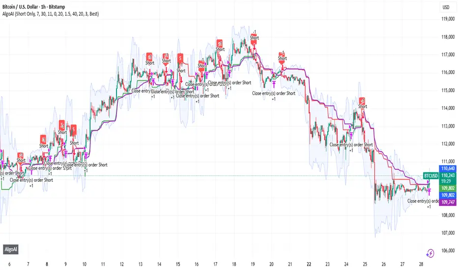
AlgoAIDESIGNED FOR HEIKEN ASHI BARS
Gain Access here: algoai.store
AlgoAI
The Dark Edge of Trading
An AI-powered TradingView strategy that thrives across all markets. Short altcoin pumps. Ride NAS100 waves. Dominate gold, FX, stocks, and futures — all with one AI brain.
#1
Semi-Automatic Trading (Recommended)
Set up alerts on AlgoAI signals. As they come in, grade the setups and choose to enter manually. This gives you full control while leveraging AI precision.
#2
Fully Automated Trading
Pass signals via webhooks to TradersPost for futures or PineConnector for FX. Note: When running fully automated, it's suggested to use long-only or short-only mode to avoid side swiping and potential unintended drawdown.
BITSTAMP:BTCUSD
Maple Trend Maximizer – AI-Powered Trend & Entry IndicatorOverview:
Maple Trend Maximizer is an AI-inspired market analysis tool that identifies trend direction, highlights high-probability entry zones, and visually guides you through market momentum. Designed for traders seeking smart, data-driven signals, it combines trend alignment with proprietary AI-style calculations for precise timing.
Key Features:
AI Trend Detection:
Automatically identifies bullish and bearish trends using advanced smoothing and trend alignment techniques.
Momentum & Signal Lines:
Dynamic lines indicate market strength and potential turning points.
Colors change to highlight high-probability entry zones.
Entry Signals:
Optional visual markers suggest precise entries when trend direction and momentum align.
Configurable to reduce noise and focus on strong setups.
Multi-Timeframe Flexibility:
Works on intraday charts or higher timeframes for swing and position trading.
Customizable Settings:
Adjustable smoothing, trend sensitivity, and signal display options.
Lets you fine-tune the indicator to your trading style.
Benefits:
Quickly identifies market direction and optimal entries.
Provides clear, visually intuitive signals.
Can be used standalone or integrated into a larger strategy system.
Maple Liquidity Hunter📌 Description for Maple Liquidity Hunter
Maple Liquidity Hunter – AI-Enhanced Volume Liquidity Detector
Maple Liquidity Hunter is an advanced volume-based indicator designed to uncover hidden liquidity zones in the market.
By dynamically analyzing price–volume interactions, it automatically highlights momentum shifts with adaptive color coding.
✨ Key Features
AI-inspired volume/price analysis model
Detects liquidity surges and potential absorption points
Auto-coloring of volume bars for quick visual recognition
Optional volume moving average filter for trend context
⚠️ Disclaimer: This tool is for educational and research purposes only. It does not guarantee future results. Always test thoroughly before live trading.

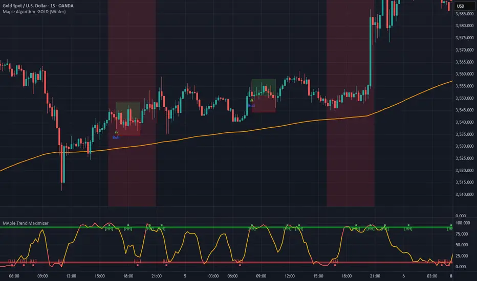
Maple Algorithm_GOLDMaple Algorithm – AI-Powered Gold Indicator
Maple Algorithm is an AI-inspired indicator designed specifically around the price behavior of Gold (XAUUSD).
It automatically calculates and plots take-profit (TP) and stop-loss (SL) levels based on dynamic market conditions, allowing traders to capture precise entries and exits.
✨ Key Features
AI-driven adaptive model trained on Gold’s market structure
Auto-generated TP/SL zones for precision trading
Compatible with your own strategies — scale from 1:2 RRR up to even higher setups
Optimized for scalping and short-term momentum bursts
⚠️ Disclaimer:
This indicator is for educational and research purposes only. It does not guarantee future results. Always test thoroughly before applying to live trading.
AI-Weighted RSI (Zeiierman)█ Overview
AI-Weighted RSI (Zeiierman) is an adaptive oscillator that enhances classic RSI by applying a correlation-weighted prediction layer. Instead of looking only at RSI values directly, this indicator continuously evaluates how other price- and volume-based features (returns, volatility, volume shifts) correlate with RSI, and then weights them accordingly to project the next RSI state.
The result is a smoother, forward-looking RSI framework that adapts to market conditions in real time.
By leveraging feature correlation instead of static formulas, AI-Weighted RSI behaves like a lightweight learning model, adjusting its emphasis depending on which features are most aligned with RSI behavior during the current regime.
█ How It Works
⚪ Feature Extraction
Each bar, the script computes features: log returns, RSI itself, ATR% (volatility), volume, and volume log-change.
⚪ Correlation Screening
Over a rolling learning window, it measures the correlation of each feature against RSI. The strongest relationships are ranked and selected.
⚪ Adaptive Weighting
Features are standardized (z-scored), then combined using their signed correlations as weights, building a rolling, adaptive prediction of RSI.
⚪ Prediction to RSI Weight
The predicted RSI is mapped back into a “weight” scale (±2 by default). Above 0 = bullish bias, below 0 = bearish bias, with color-graded fills to visualize overbought/oversold pressure.
⚪ Signal Line
A smoothing option (signal length) overlays a moving average of the AI-Weighted RSI for clearer trend confirmation.
█ Why AI-Weighted RSI
⚪ Adaptive to Market Regime
Because the model re-evaluates correlations continuously, it naturally shifts which features dominate, sometimes volatility explains RSI best, sometimes volume, sometimes returns.
⚪ Forward-Looking Bias
Instead of simply reflecting RSI, the model provides a projection, helping anticipate shifts in momentum before RSI itself flips.
█ How to Use
⚪ Directional Bias
Read the RSI relative to 0. Above = bullish momentum bias, below = bearish.
⚪ Overbought / Oversold Zones
Shaded fills beyond +0.5 or -0.5 highlight extremes where RSI pressure often exhausts.
⚪ Divergences
When price makes new highs/lows but AI-Weighted RSI fails to confirm, it often signals weakening momentum.
█ Settings
RSI Length: Lookback for the core RSI calculation.
Signal Length: Smoothing applied to the AI-Weighted RSI output.
Learning Window: Bars used for correlation learning and z-scoring.
-----------------
Disclaimer
The content provided in my scripts, indicators, ideas, algorithms, and systems is for educational and informational purposes only. It does not constitute financial advice, investment recommendations, or a solicitation to buy or sell any financial instruments. I will not accept liability for any loss or damage, including without limitation any loss of profit, which may arise directly or indirectly from the use of or reliance on such information.
All investments involve risk, and the past performance of a security, industry, sector, market, financial product, trading strategy, backtest, or individual's trading does not guarantee future results or returns. Investors are fully responsible for any investment decisions they make. Such decisions should be based solely on an evaluation of their financial circumstances, investment objectives, risk tolerance, and liquidity needs.

Racktor Analysis Assistant
Racktor Analysis Assistant — Feature Overview
The Racktor Analysis Assistant is a multi-module market-structure toolkit that plots pivots, BoS/ChoCh levels, session breakouts, inside bars, and higher-timeframe BTS/STB trap signals — with complete styling controls and alerting.
Smart Pivot Engine (ZigZag Core)
- Adaptive pivot period switching based on timeframe threshold.
- ZigZag stream tracks pivot types (H/L, HH/HL/LH/LL) with Major & Minor streams.
- Clean visuals: optional ZigZag line & pivot labels with customizable style, width, and color.
Major & Minor Structure Signals
- Detects BoS and ChoCh for both Major and Minor swings.
- Updates External Trend on Major events and Internal Trend on Minor events.
- One-time triggers per level via locking.
- Per-category styling for Major/Minor Bullish & Bearish BoS and ChoCh.
- Alerts with symbol, pivot, timeframe, and time, limited to specific timeframes if desired.
Inside Bar Module
- Toggleable Inside Bar detection.
- Custom colors for bullish and bearish inside bars.
- Optional alerts on detection.
Session Breakout Suite
- Custom session window with shaded box.
- On session close, plots High/Mid/Low breakout lines extendable for N hours.
- Optional previous day & week high/low lines.
- Breakout vs Liquidity Sweep modes (close-based or wick-based confirmation).
- Display styles: Fixed (triangles) or Moving (vertical dotted lines).
- Alerts for “first event” or “every event.”
BTS/STB Trap (Higher-Timeframe ID1/ID2 Logic)
- BTS/STB toggle with selectable check timeframe (default: 4H).
- STB (bullish, Sell→Buy): strict ID1/ID2 relationships, both candles bullish; green circle below HTF ID1 low.
- BTS (bearish, Buy→Sell): strict ID1/ID2 relationships, both candles bearish; red circle above HTF ID1 high.
- Non-repainting; dots appear only at HTF candle close.
- Timeframe-aware rendering (dots show only on selected timeframe).
- Alerts for STB/BTS at HTF close.
Styling & Limits
- Per-feature color/style/width customization.
- Generous limits for boxes, labels, and lines.
- Session tools limited to ≤ 120-minute charts for accuracy.
Anti-Repaint
- HTF signals use lookahead_off and HTF-close gating to avoid repainting.
- BoS/ChoCh and Session logic track prior values and use locks to prevent duplicates.
Quick Start
Set the Timeframe Threshold and pivot periods for lower/higher TFs.
Enable desired Major/Minor BoS/ChoCh lines and customize styles.
Activate Inside Bar Module if required.
Configure Session Breakout window, mode, and alert settings.
Enable BTS/STB detection, keeping 4H default or selecting a custom TF.
Add alerts for chosen signals and let the assistant annotate structure, sessions, and HTF traps.
Best Use with Racktor's Core Trading Strategy
For traders who want structure clarity without clutter, this Analysis-Assistant is built to keep your chart actionable and adaptive.

ICT AI ATR Signals [TradingFinder]🔵 Introduction
In financial markets, two main factors always have the greatest impact on traders’ decisions: the direction of the trend and the level of price volatility. Although there are various tools to analyze each of these factors, very few indicators can combine them in a coordinated and simultaneous way.
The ICT AI ATR indicator has been designed with this purpose in mind, to provide a unified and comprehensive view of the market instead of relying on multiple scattered indicators.
This indicator is built upon two widely used tools: the Moving Average (MA) and the Average True Range (ATR). The combination of these two indicators allows traders to simultaneously track the trend direction and account for market volatility two elements that always play a decisive role in trading decisions.
In the structure of the indicator, the Moving Average acts as the central line and serves as the backbone of the tool. By calculating the average price over a defined period, the Moving Average filters out excess market noise and provides a clearer picture of the overall price movement.
This helps traders focus on the main trend instead of being distracted by minor and temporary fluctuations. The central line is thus the main reference point for identifying the trend direction.
Alongside this, the ATR is responsible for measuring the real volatility of the market. Unlike many tools that only look at closing price changes, the ATR considers the true range of candlestick movements, giving a more accurate view of market dynamics.
In the ICT AI ATR indicator, this feature is used to draw dynamic bands above and below the Moving Average line. These bands shift with changing market conditions and act like dynamic support and resistance levels, areas where strong price reactions often occur.
This combination allows traders not only to see the dominant market trend through the Moving Average but also to understand volatility and the natural price range via the ATR. For this reason, the ICT AI ATR identifies points that are likely to act as reaction or reversal zones, whether during bounces off the bands or breakouts through them.
With this structure, the trader can at a glance :
Identify the overall market direction using the Moving Average.
Observe volatility and the natural range of price movement through ATR.
Recognize key levels where strong reactions or potential reversals are more likely.
As a result, the ICT AI ATR functions as a combined tool that replaces the need to use several separate indicators, enabling traders to analyze trend, volatility, price bands, and even Fibonacci targets within a single unified framework.
🔵 How to Use
The ICT AI ATR indicator is designed to simplify market analysis through two main components: visual display of bands and signals on the chart itself, and a multi-symbol analytical dashboard capable of monitoring over 20 different assets simultaneously across multiple timeframes.
This dashboard feature allows traders to gain a quick overview of overall market conditions without opening multiple charts or constantly switching timeframes. It updates in real-time, showing active Buy (Long) and Sell signals for each symbol.
As such, the combination of direct chart display and dashboard analytics makes the indicator useful both for detailed analysis of a single symbol and for monitoring multiple markets at once.
🟣 How do ICT AI ATR trading signals work?
Sell Signal (Short) : Triggered when the price pushes below the lower band (Low goes outside the lower band) and then closes back above it. This indicates potential weakness in bullish momentum and suggests possible selling pressure or the start of a downward correction. Traders can use this to spot sell setups or manage long positions.
Buy Signal (Long) : Triggered when the price extends above the upper band (High goes outside the upper band) and then closes back below it. This often signals exhaustion in bearish pressure and the return of buying strength, potentially marking the start of a new upward move.
This signaling logic is based on the actual behavior of price relative to the ATR dynamic bands. Unlike static formulas, signals adapt to changing market conditions, making them more accurate and reliable.
The main advantage of the ICT AI ATR indicator is that traders can benefit from real-time analysis directly on the chart by observing price interactions with the bands and signals while also receiving a multi-market overview through the dashboard. This combination is especially valuable for traders who operate across multiple instruments or markets simultaneously.
🔵 Settings
🟣 Logical settings
Moving Average Type : Select the type of moving average for the central line. Options include EMA, SMA, RMA, WMA, or HMA depending on the trading strategy.
Moving Average Period : Defines the length of the moving average. Shorter periods make the central line more responsive to price changes, while longer periods smooth out the line to show the broader trend.
ATR Period : Determines the number of candles considered for volatility calculation. Shorter periods increase sensitivity, while longer periods provide a more stable view of volatility.
ATR Multiplier : Sets the distance between the upper/lower bands and the central moving average line. Higher values widen the bands, while lower values bring them closer to price.
Smooth Period: Used to smooth data and reduce chart noise. Higher values produce smoother, more consistent indicator lines.
Signal Gap : Defines the minimum number of candles required between two consecutive signals. This prevents back-to-back signals from appearing too frequently and ensures only the more reliable ones are shown.
🟣 Display Settings
Table on Chart : Allows users to choose the position of the signal dashboard either directly on the chart or below it, depending on their layout preference.
Number of Symbols : Enables users to control how many symbols are displayed in the screener table, from 10 to 20, adjustable in increments of 2 symbols for flexible screening depth.
Table Mode : This setting offers two layout styles for the signal table :
Basic : Mode displays symbols in a single column, using more vertical space.
Extended : Mode arranges symbols in pairs side-by-side, optimizing screen space with a more compact view.
Table Size : Lets you adjust the table’s visual size with options such as: auto, tiny, small, normal, large, huge.
Table Position : Sets the screen location of the table. Choose from 9 possible positions, combining vertical (top, middle, bottom) and horizontal (left, center, right) alignments.
🟣 Symbol Settings
Each of the 10 symbol slots comes with a full set of customizable parameters :
Symbol : Define or select the asset (e.g., XAUUSD, BTCUSD, EURUSD, etc.).
Timeframe : Set your desired timeframe for each symbol (e.g., 15, 60, 240, 1D).
🟣 Alert Settings
Alert : Enables alerts for AAS.
Message Frequency : Determines the frequency of alerts. Options include 'All' (every function call), 'Once Per Bar' (first call within the bar), and 'Once Per Bar Close' (final script execution of the real-time bar). Default is 'Once per Bar'.
Show Alert Time by Time Zone : Configures the time zone for alert messages. Default is 'UTC'.
🔵 Conclusion
The ICT AI ATR indicator, by combining three core elements Moving Average for trend detection, ATR for volatility measurement and dynamic bands, and Fibonacci levels for price targets—provides a multi-layered and intelligent tool for market analysis. In addition to showing accurate bands directly on the chart, it also offers a multi-symbol dashboard that allows traders to monitor signals across different assets and timeframes in real time.
The key advantage of this indicator is that it eliminates the need to use several separate tools by integrating trend, volatility, key levels, and trade signals into one unified framework. For this reason, ICT AI ATR is a reliable and effective choice for both short-term traders seeking quick market moves and long-term traders focused on dynamic support and resistance levels.
Paid script

Machine Learning BBPct [BackQuant]Machine Learning BBPct
What this is (in one line)
A Bollinger Band %B oscillator enhanced with a simplified K-Nearest Neighbors (KNN) pattern matcher. The model compares today’s context (volatility, momentum, volume, and position inside the bands) to similar situations in recent history and blends that historical consensus back into the raw %B to reduce noise and improve context awareness. It is informational and diagnostic—designed to describe market state, not to sell a trading system.
Background: %B in plain terms
Bollinger %B measures where price sits inside its dynamic envelope: 0 at the lower band, 1 at the upper band, ~ 0.5 near the basis (the moving average). Readings toward 1 indicate pressure near the envelope’s upper edge (often strength or stretch), while readings toward 0 indicate pressure near the lower edge (often weakness or stretch). Because bands adapt to volatility, %B is naturally comparable across regimes.
Why add (simplified) KNN?
Classic %B is reactive and can be whippy in fast regimes. The simplified KNN layer builds a “nearest-neighbor memory” of recent market states and asks: “When the market looked like this before, where did %B tend to be next bar?” It then blends that estimate with the current %B. Key ideas:
• Feature vector . Each bar is summarized by up to five normalized features:
– %B itself (normalized)
– Band width (volatility proxy)
– Price momentum (ROC)
– Volume momentum (ROC of volume)
– Price position within the bands
• Distance metric . Euclidean distance ranks the most similar recent bars.
• Prediction . Average the neighbors’ prior %B (lagged to avoid lookahead), inverse-weighted by distance.
• Blend . Linearly combine raw %B and KNN-predicted %B with a configurable weight; optional filtering then adapts to confidence.
This remains “simplified” KNN: no training/validation split, no KD-trees, no scaling beyond windowed min-max, and no probabilistic calibration.
How the script is organized (by input groups)
1) BBPct Settings
• Price Source – Which price to evaluate (%B is computed from this).
• Calculation Period – Lookback for SMA basis and standard deviation.
• Multiplier – Standard deviation width (e.g., 2.0).
• Apply Smoothing / Type / Length – Optional smoothing of the %B stream before ML (EMA, RMA, DEMA, TEMA, LINREG, HMA, etc.). Turning this off gives you the raw %B.
2) Thresholds
• Overbought/Oversold – Default 0.8 / 0.2 (inside ).
• Extreme OB/OS – Stricter zones (e.g., 0.95 / 0.05) to flag stretch conditions.
3) KNN Machine Learning
• Enable KNN – Switch between pure %B and hybrid.
• K (neighbors) – How many historical analogs to blend (default 8).
• Historical Period – Size of the search window for neighbors.
• ML Weight – Blend between raw %B and KNN estimate.
• Number of Features – Use 2–5 features; higher counts add context but raise the risk of overfitting in short windows.
4) Filtering
• Method – None, Adaptive, Kalman-style (first-order),
or Hull smoothing.
• Strength – How aggressively to smooth. “Adaptive” uses model confidence to modulate its alpha: higher confidence → stronger reliance on the ML estimate.
5) Performance Tracking
• Win-rate Period – Simple running score of past signal outcomes based on target/stop/time-out logic (informational, not a robust backtest).
• Early Entry Lookback – Horizon for forecasting a potential threshold cross.
• Profit Target / Stop Loss – Used only by the internal win-rate heuristic.
6) Self-Optimization
• Enable Self-Optimization – Lightweight, rolling comparison of a few canned settings (K = 8/14/21 via simple rules on %B extremes).
• Optimization Window & Stability Threshold – Governs how quickly preferred K changes and how sensitive the overfitting alarm is.
• Adaptive Thresholds – Adjust the OB/OS lines with volatility regime (ATR ratio), widening in calm markets and tightening in turbulent ones (bounded 0.7–0.9 and 0.1–0.3).
7) UI Settings
• Show Table / Zones / ML Prediction / Early Signals – Toggle informational overlays.
• Signal Line Width, Candle Painting, Colors – Visual preferences.
Step-by-step logic
A) Compute %B
Basis = SMA(source, len); dev = stdev(source, len) × multiplier; Upper/Lower = Basis ± dev.
%B = (price − Lower) / (Upper − Lower). Optional smoothing yields standardBB .
B) Build the feature vector
All features are min-max normalized over the KNN window so distances are in comparable units. Features include normalized %B, normalized band width, normalized price ROC, normalized volume ROC, and normalized position within bands. You can limit to the first N features (2–5).
C) Find nearest neighbors
For each bar inside the lookback window, compute the Euclidean distance between current features and that bar’s features. Sort by distance, keep the top K .
D) Predict and blend
Use inverse-distance weights (with a strong cap for near-zero distances) to average neighbors’ prior %B (lagged by one bar). This becomes the KNN estimate. Blend it with raw %B via the ML weight. A variance of neighbor %B around the prediction becomes an uncertainty proxy ; combined with a stability score (how long parameters remain unchanged), it forms mlConfidence ∈ . The Adaptive filter optionally transforms that confidence into a smoothing coefficient.
E) Adaptive thresholds
Volatility regime (ATR(14) divided by its 50-bar SMA) nudges OB/OS thresholds wider or narrower within fixed bounds. The aim: comparable extremeness across regimes.
F) Early entry heuristic
A tiny two-step slope/acceleration probe extrapolates finalBB forward a few bars. If it is on track to cross OB/OS soon (and slope/acceleration agree), it flags an EARLY_BUY/SELL candidate with an internal confidence score. This is explicitly a heuristic—use as an attention cue, not a signal by itself.
G) Informational win-rate
The script keeps a rolling array of trade outcomes derived from signal transitions + rudimentary exits (target/stop/time). The percentage shown is a rough diagnostic , not a validated backtest.
Outputs and visual language
• ML Bollinger %B (finalBB) – The main line after KNN blending and optional filtering.
• Gradient fill – Greenish tones above 0.5, reddish below, with intensity following distance from the midline.
• Adaptive zones – Overbought/oversold and extreme bands; shaded backgrounds appear at extremes.
• ML Prediction (dots) – The KNN estimate plotted as faint circles; becomes bright white when confidence > 0.7.
• Early arrows – Optional small triangles for approaching OB/OS.
• Candle painting – Light green above the midline, light red below (optional).
• Info panel – Current value, signal classification, ML confidence, optimized K, stability, volatility regime, adaptive thresholds, overfitting flag, early-entry status, and total signals processed.
Signal classification (informational)
The indicator does not fire trade commands; it labels state:
• STRONG_BUY / STRONG_SELL – finalBB beyond extreme OS/OB thresholds.
• BUY / SELL – finalBB beyond adaptive OS/OB.
• EARLY_BUY / EARLY_SELL – forecast suggests a near-term cross with decent internal confidence.
• NEUTRAL – between adaptive bands.
Alerts (what you can automate)
• Entering adaptive OB/OS and extreme OB/OS.
• Midline cross (0.5).
• Overfitting detected (frequent parameter flipping).
• Early signals when early confidence > 0.7.
These are purely descriptive triggers around the indicator’s state.
Practical interpretation
• Mean-reversion context – In range markets, adaptive OS/OB with ML smoothing can reduce whipsaws relative to raw %B.
• Trend context – In persistent trends, the KNN blend can keep finalBB nearer the mid/upper region during healthy pullbacks if history supports similar contexts.
• Regime awareness – Watch the volatility regime and adaptive thresholds. If thresholds compress (high vol), “OB/OS” comes sooner; if thresholds widen (calm), it takes more stretch to flag.
• Confidence as a weight – High mlConfidence implies neighbors agree; you may rely more on the ML curve. Low confidence argues for de-emphasizing ML and leaning on raw %B or other tools.
• Stability score – Rising stability indicates consistent parameter selection and fewer flips; dropping stability hints at a shifting backdrop.
Methodological notes
• Normalization uses rolling min-max over the KNN window. This is simple and scale-agnostic but sensitive to outliers; the distance metric will reflect that.
• Distance is unweighted Euclidean. If you raise featureCount, you increase dimensionality; consider keeping K larger and lookback ample to avoid sparse-neighbor artifacts.
• Lag handling intentionally uses neighbors’ previous %B for prediction to avoid lookahead bias.
• Self-optimization is deliberately modest: it only compares a few canned K/threshold choices using simple “did an extreme anticipate movement?” scoring, then enforces a stability regime and an overfitting guard. It is not a grid search or GA.
• Kalman option is a first-order recursive filter (fixed gain), not a full state-space estimator.
• Hull option derives a dynamic length from 1/strength; it is a convenience smoothing alternative.
Limitations and cautions
• Non-stationarity – Nearest neighbors from the recent window may not represent the future under structural breaks (policy shifts, liquidity shocks).
• Curse of dimensionality – Adding features without sufficient lookback can make genuine neighbors rare.
• Overfitting risk – The script includes a crude overfitting detector (frequent parameter flips) and will fall back to defaults when triggered, but this is only a guardrail.
• Win-rate display – The internal score is illustrative; it does not constitute a tradable backtest.
• Latency vs. smoothness – Smoothing and ML blending reduce noise but add lag; tune to your timeframe and objectives.
Tuning guide
• Short-term scalping – Lower len (10–14), slightly lower multiplier (1.8–2.0), small K (5–8), featureCount 3–4, Adaptive filter ON, moderate strength.
• Swing trading – len (20–30), multiplier ~2.0, K (8–14), featureCount 4–5, Adaptive thresholds ON, filter modest.
• Strong trends – Consider higher adaptive_upper/lower bounds (or let volatility regime do it), keep ML weight moderate so raw %B still reflects surges.
• Chop – Higher ML weight and stronger Adaptive filtering; accept lag in exchange for fewer false extremes.
How to use it responsibly
Treat this as a state descriptor and context filter. Pair it with your execution signals (structure breaks, volume footprints, higher-timeframe bias) and risk management. If mlConfidence is low or stability is falling, lean less on the ML line and more on raw %B or external confirmation.
Summary
Machine Learning BBPct augments a familiar oscillator with a transparent, simplified KNN memory of recent conditions. By blending neighbors’ behavior into %B and adapting thresholds to volatility regime—while exposing confidence, stability, and a plain early-entry heuristic—it provides an informational, probability-minded view of stretch and reversion that you can interpret alongside your own process.
Lorentzian Key Support and Resistance Level Detector [mishy]🧮 Lorentzian Key S/R Levels Detector
Advanced Support & Resistance Detection Using Mathematical Clustering
The Problem
Traditional S/R indicators fail because they're either subjective (manual lines), rigid (fixed pivots), or break when price spikes occur. Most importantly, they don't tell you where prices actually spend time, just where they touched briefly.
The Solution: Lorentzian Distance Clustering
This indicator introduces a novel approach by using Lorentzian distance instead of traditional Euclidean distance for clustering. This is groundbreaking for financial data analysis.
Data Points Clustering:
🔬 Why Euclidean Distance Fails in Trading
Traditional K-means uses Euclidean distance:
• Formula: distance = (price_A - price_B)²
• Problem: Squaring amplifies differences exponentially
• Real impact: One 5% price spike has 25x more influence than a 1% move
• Result: Clusters get pulled toward outliers, missing real support/resistance zones
Example scenario:
Prices: ← flash spike
Euclidean: Centroid gets dragged toward 150
Actual S/R zone: Around 100 (where prices actually trade)
⚡ Lorentzian Distance: The Game Changer
Our approach uses Lorentzian distance:
• Formula: distance = log(1 + (price_difference)² / σ²)
• Breakthrough: Logarithmic compression keeps outliers in check
• Real impact: Large moves still matter, but don't dominate
• Result: Clusters focus on where prices actually spend time
Same example with Lorentzian:
Prices: ← flash spike
Lorentzian: Centroid stays near 100 (real trading zone)
Outlier (150): Acknowledged but not dominant
🧠 Adaptive Intelligence
The σ parameter isn't fixed,it's calculated from market disturbance/entropy:
• High volatility: σ increases, making algorithm more tolerant of large moves
• Low volatility: σ decreases, making algorithm more sensitive to small changes
• Self-calibrating: Adapts to any instrument or market condition automatically
Why this matters: Traditional methods treat a 2% move the same whether it's in a calm or volatile market. Lorentzian adapts the sensitivity based on current market behavior.
🎯 Automatic K-Selection (Elbow Method)
Instead of guessing how many S/R levels to draw, the indicator:
• Tests 2-6 clusters and calculates WCSS (tightness measure)
• Finds the "elbow" - where adding more clusters stops helping much
• Uses sharpness calculation to pick the optimal number automatically
Result: Perfect balance between detail and clarity.
How It Works
1. Collect recent closing prices
2. Calculate entropy to adapt to current market volatility
3. Cluster prices using Lorentzian K-means algorithm
4. Auto-select optimal cluster count via statistical analysis
5. Draw levels at cluster centers with deviation bands
📊 Manual K-Selection Guide (Using WCSS & Sharpness Analysis)
When you disable auto-selection, use both WCSS and Sharpness metrics from the analysis table to choose manually:
What WCSS tells you:
• Lower WCSS = tighter clusters = better S/R levels
• Higher WCSS = scattered clusters = weaker levels
What Sharpness tells you:
• Higher positive values = optimal elbow point = best K choice
• Lower/negative values = poor elbow definition = avoid this K
• Measures the "sharpness" of the WCSS curve drop-off
Decision strategy using both metrics:
K=2: WCSS = 150.42 | Sharpness = - | Selected =
K=3: WCSS = 89.15 | Sharpness = 22.04 | Selected = ✓ ← Best choice
K=4: WCSS = 76.23 | Sharpness = 1.89 | Selected =
K=5: WCSS = 73.91 | Sharpness = 1.43 | Selected =
Quick decision rules:
• Pick K with highest positive Sharpness (indicates optimal elbow)
• Confirm with significant WCSS drop (30%+ reduction is good)
• Avoid K values with negative or very low Sharpness (<1.0)
• K=3 above shows: Big WCSS drop (41%) + High Sharpness (22.04) = Perfect choice
Why this works:
The algorithm finds the "elbow" where adding more clusters stops being useful. High Sharpness pinpoints this elbow mathematically, while WCSS confirms the clustering quality.
Elbow Method Visualization:
Traditional clustering problems:
❌ Price spikes distort results
❌ Fixed parameters don't adapt
❌ Manual tuning is subjective
❌ No way to validate choices
Lorentzian solution:
☑️ Outlier-resistant distance metric
☑️ Entropy-based adaptation to volatility
☑️ Automatic optimal K selection
☑️ Statistical validation via WCSS & Sharpness
Features
Visual:
• Color-coded levels (red=highest resistance, green=lowest support)
• Optional deviation bands showing cluster spread
• Strength scores on labels: Each cluster shows a reliability score.
• Higher scores (0.8+) = very strong S/R levels with tight price clustering
• Lower scores (0.6-0.7) = weaker levels, use with caution
• Based on cluster tightness and data point density
• Clean line extensions and labels
Analytics:
• WCSS analysis table showing why K was chosen
• Cluster metrics and statistics
• Real-time entropy monitoring
Control:
• Auto/manual K selection toggle
• Customizable sample size (20-500 bars)
• Show/hide bands and metrics tables
The Result
You get mathematically validated S/R levels that focus on where prices actually cluster, not where they randomly spiked. The algorithm adapts to market conditions and removes guesswork from level selection.
Best for: Traders who want objective, data-driven S/R levels without manual chart analysis.
Credits: This script is for educational purposes and is inspired by the work of @ThinkLogicAI and an amazing mentor @DskyzInvestments . It demonstrates how Lorentzian geometrical concepts can be applied not only in ML classification but also quite elegantly in clustering.

AI Breakout Bands (Zeiierman)█ Overview
AI Breakout Bands (Zeiierman) is an adaptive trend and breakout detection system that combines Kalman filtering with advanced K-Nearest Neighbor (KNN) smoothing. The result is a smart, self-adjusting band structure that adapts to dynamic market behavior, identifying breakout conditions with precision and visual clarity.
At its core, this indicator estimates price behavior using a two-dimensional Kalman filter (position + velocity), then enhances the smoothing process with a nonlinear, similarity-based KNN filter. This unique blend enables it to handle noisy markets and directional shifts with both speed and stability — providing breakout traders and trend followers a reliable framework to act on.
Whether you're identifying volatility expansions, capturing trend continuations, or spotting early breakout conditions, AI Breakout Bands gives you a mathematically grounded, visually adaptive roadmap of real-time market structure.
█ How It Works
⚪ Kalman Filter Engine
The Kalman filter models price movement as a state system with two components:
Position (price)
Velocity (trend direction)
It recursively updates predictions using real-time price as a noisy observation, balancing responsiveness with smoothness.
Process Noise (Position) controls sensitivity to sudden moves.
Process Noise (Velocity) controls smoothing of directional flow.
Measurement Noise (R) defines how much the filter "trusts" live price data.
This component alone creates a responsive yet stable estimate of the market’s center of gravity.
⚪ Advanced K-Neighbor Smoothing
After the Kalman estimate is computed, the script applies a custom K-Nearest Neighbor (KNN) smoother.
Rather than averaging raw values, this method:
Finds K most similar past Kalman values
Weighs them by similarity (inverse of absolute distance)
Produces a smoother that emphasizes structural similarity
This nonlinear approach gives the indicator an AI feature — reacting fast when needed, yet staying calm in consolidation.
█ How to Use
⚪ Trend Recognition
The line color shifts dynamically based on slope direction and breakout confirmation.
Bullish conditions: price above the mid band with positive slope
Bearish conditions: price below the mid band with negative slope
⚪ Breakout Signals
Price breaking above or below the bands may signal momentum acceleration.
Combine with your own volume or momentum confirmation for stronger entries.
Bands adapt to market noise, helping filter out low-quality whipsaws.
█ Settings
Process Noise (Position): Controls Kalman filter’s sensitivity to price changes.
Process Noise (Velocity): Controls smoothing of directional component.
Measurement Noise (R): Defines how much trust is placed in price data.
K-Neighbor Length: Number of historical Kalman values considered for smoothing.
Slope Calculation Window: Number of bars used to compute trend slope of the smoothed Kalman.
Band Lookback (MAE): Rolling period for average absolute error.
Band Multiplier: Multiplies MAE to determine band width.
-----------------
Disclaimer
The content provided in my scripts, indicators, ideas, algorithms, and systems is for educational and informational purposes only. It does not constitute financial advice, investment recommendations, or a solicitation to buy or sell any financial instruments. I will not accept liability for any loss or damage, including without limitation any loss of profit, which may arise directly or indirectly from the use of or reliance on such information.
All investments involve risk, and the past performance of a security, industry, sector, market, financial product, trading strategy, backtest, or individual's trading does not guarantee future results or returns. Investors are fully responsible for any investment decisions they make. Such decisions should be based solely on an evaluation of their financial circumstances, investment objectives, risk tolerance, and liquidity needs.

ML: Lorentzian Classification Premium█ OVERVIEW
Lorentzian Classification Premium represents the culmination of two years of collaborative development with over 1,000 beta testers from the TradingView community. Building upon the foundation of the open-source version, this premium edition introduces powerful enhancements that transform how machine-learning classification can be applied to market analysis.
The premium version maintains the core Lorentzian distance-based classification algorithm while expanding its capabilities through triple the feature dimensionality (up to 15 features), sophisticated mean-reversion detection, first-pullback identification, and a comprehensive signal taxonomy that goes far beyond simple buy/sell signals. Whether you're building automated trading systems, conducting deep market research, or integrating proprietary indicators into ML workflows, this tool provides the advanced edge needed for professional-grade analysis.
█ BACKGROUND
Lorentzian Classification analyzes market structures, especially those exhibiting non-linear distortions under stress, by employing advanced distance metrics like the Lorentzian metric, prominent in fields such as relativity theory. Where traditional indicators assume flat space, we embrace the curve. The heart of this approach is the Lorentzian distance metric—a sophisticated mathematical tool. This framework adeptly navigates the complex curves and distortions of market space, aiming to provide insights that traditional analysis might miss, especially during moments of extreme volatility. It analyzes historical data from a multi-dimensional feature space consisting of various technical indicators of your choosing. Where traditional approaches fail, Lorentzian space reveals the true geometry of market dynamics.
Neighborhoods in Different Geometries: In the above figure, the Lorentzian metric creates distinctive cross-patterns aligned with feature axes (RSI, CCI, ADX), capturing both local similarity and dimensional extremes. This unique geometry allows the algorithm to recognize similar market conditions that Euclidean spheres and Manhattan diamonds would miss entirely. In LC Premium, users can have up to 15 features -- you are not limited to 3-dimensions.
Among the thousands of distance metrics discovered by mathematicians, each perceives data through its own geometric lens. The Lorentzian metric stands apart with its unique ability to capture market behavior during volatile events.
█ COMMUNITY-DRIVEN EVOLUTION
It has been profoundly humbling over the past 2 years to witness this indicator's evolution through the collaborative efforts of our incredible community. This journey has been shaped by thousands of user suggestions and validated through real-world application.
A particularly amazing milestone was the development of a complete community-driven Python port, which meticulously matched even the most minute PineScript quirks. Building on this solid foundation, a new command-line interface (CLI) has opened up exciting possibilities for chart-specific parameter optimization:
Early insights from parameter optimization research: Through grid-search testing across thousands of parameter combinations, the analysis identifies which parameters have the biggest effects on performance and maps regions of stability across different market regimes. This reveals that optimal neighbor counts vary significantly based on market conditions—opening up incredible potential for timeframe-specific optimization.
This is just one of the insights gleaned so far from this ongoing investigation. The potential for chart-specific optimization for any given timeframe could transform how traders approach parameter selection.
Demand from power users for extra capabilities—while keeping the open-source version simple—sparked this Premium release. The open-source branch remains maintained, but the premium tier adds unique features for those who need an analytical edge and to leverage their own custom indicators as feature series for the algorithm.
█ KEY PREMIUM FEATURES
📈 First Pullback Detection System
Automatically identifies high-probability trend-continuation entries after initial momentum moves.
Detects when price retraces to optimal entry zones following breakouts or trend initiations.
Green/red triangle signals often fire before main classification arrows.
Dedicated alerts for both bullish and bearish pullback opportunities.
Based on veryfid's extensive research into pullback mechanics and market structure.
🔄 Dynamic Kernel Regression Envelope
Powerful, zero-setup confluence layer that immediately communicates trend shifts.
Dual-kernel system creates a visual envelope between trend estimates.
Color gradient dynamically represents prediction strength and market conviction.
Crossovers provide additional confirmation without cluttering your chart.
Professional visualization that rivals institutional-grade analysis tools.
✨ Massively Expanded Dimensionality: 10 Custom Sources, 5 Built-In Sources
Transform the indicator from 5 built-in standard to 15 total total features—triple the analytical power.
Integrate ANY TradingView indicator as a machine learning feature.
Built-in normalization ensures all indicators contribute equally regardless of scale.
Create theme-based systems: pure volume analysis, multi-timeframe momentum, or hybrid approaches.
📊 Tiered Mean Reversion Signals with Scalping Alerts
Regular (🔄) and Strong (⬇️/⬆️) mean reversion signals based on statistical extremes.
Opportunities often arise before candle close—perfect for scalping entries.
Visual markers appear at high-probability reversal zones.
Four specialized alert types: upward/downward for both regular and strong reversals.
Pre-optimized probability thresholds, no fine-tuning required.
📅 Daily Kernel Trend Filter
Instantly cleans up noisy intraday charts by aligning with higher timeframe trends.
Swing traders report immediate signal quality improvement.
Automatically deactivates on daily+ timeframes (intelligent context awareness).
Reduces counter-trend signals by up to 60% on lower timeframes.
Simple toggle—no complex multi-timeframe setup required.
📋 Professional Backtesting Stream (-6 to +6)
Multiple distinct signal types (including pullbacks, mean reversions, and kernel deviations) vs. basic binary (buy/sell) output for nuanced analysis.
Enables detailed walk-forward analysis and ML model training.
Compatible with external backtesting frameworks via numeric stream.
Rare precision for TradingView indicators—usually only found in institutional tools.
Perfect for quants building sophisticated strategy layers.
⚡ Performance Optimizations
Faster distance calculations through algorithmic improvements.
Reduced indicator load time (measured via Pine Profiler).
Handles 15 active features without timeouts—critical for multi-chart setups.
Optimized for live auto-trading bots requiring minimal latency.
🎨 Full Visual Customization & Accessibility
Complete color control for all visual elements.
Colorblind-safe default palette with customization options.
Dark mode optimization for extended trading sessions.
Professional appearance matching your trading workspace.
Accessibility features meeting modern UI standards.
🛠️ Advanced Training Modes
Downsampling mode for training on diverse market conditions; Down-sampling and remote-fractals for exotic pattern discovery.
Remote fractals option extends analysis to deep historical patterns.
Reset factor control for fine-tuning neighbor diversity; Reset-factor tuning to control neighbor diversity.
Appeals to systematic traders exploring exotic data approaches.
Prevents temporal clustering bias in model training.
█ HOW TO USE
Understanding the Approach (Core Concept):
Lorentzian Classification uses a k-Nearest Neighbors (k-NN) algorithm. It searches for historical price action "neighborhoods" similar to the current market state. Instead of a simple straight-line (Euclidean) distance, it primarily uses a Lorentzian distance metric, which can account for market "warping" or distortions often seen during high volatility or significant events. Each historical neighbor "votes" on what happened next in its context, and these votes aggregate into a classification score for the current bar.
Interpreting Bar Scores & Signals (Interpreting the Chart):
Bar Prediction Values: Numbers over each candle (e.g., ranging from -8 to +8 if Neighbors Count is 8) represent the aggregated vote from the nearest neighbors. Strong positive scores (e.g., +7, +8) indicate a strong bullish consensus among historical analogs. Strong negative scores (e.g., -7, -8) indicate a strong bearish consensus. Scores near zero suggest neutrality or conflicting signals from neighbors. The intensity of bar colors (if Use Confidence Gradient is on) often reflects these scores.
Main Arrows (Main Buy/Sell Labels): Large ▲/▼ labels are the primary entry signals generated when the overall classification (after filters) is bullish or bearish.
Pullback Triangles: Small green/red ▲/▼ identify potential trend continuation entries. These signals often appear after an initial price move and a subsequent minor retracement, suggesting the trend might resume. This is based on recognizing patterns where a brief counter-movement is followed by a continued advance in the initial trend direction.
Mean-Reversion Symbols: 🔄 (Regular Reversion) appears when price has crossed the average band of the Dynamic Kernel Regression Envelope. ⬇️/⬆️ (Strong Reversion) means price has crossed the far band of the envelope, indicating a more extreme deviation and potentially a stronger reversion opportunity.
Custom Mean Reversion Deviation Markers (Deviation Dots): If Enable Custom Mean Reversion Alerts is on, these dots appear when price deviates from the main kernel regression line by a user-defined ATR multiple, signaling a custom-defined reversion opportunity.
Kernel Regression Lines & Envelope: The Main Kernel Estimate (thicker line) is an adaptive moving average that smooths price and helps identify trend direction. Its color indicates the current trend bias. The Envelope (outer bands and a midline) creates a channel around price, and its interaction with price generates mean reversion signals.
Key Input Groups & Their Purpose:
🔧 GENERAL SETTINGS:
Reduce Price-Time Warping : Toggles the distance metric. When enabled, it reduces the characteristic "warping" effect of the default Lorentzian metric, making the distance calculation more Euclidean in nature. This may be suited for periods exhibiting less pronounced price-time distortions.
Source : Price data for calculations (default: close ).
Neighbors Count : The 'k' in k-NN – number of historical analogs considered.
Max Bars Back : How far back the indicator looks for historical patterns.
Show Exits / Use Dynamic Exits : Controls visibility and logic for exit signals.
Include Full History (Use Remote Fractals) : Allows model to pick "exotic" fractals from deep chart history.
Use Downsampling / Reset Factor : Advanced training parameters affecting neighbor selection.
Show Trade Stats / Use Worst Case Estimates : Displays a real-time performance table (for calibration only).
🎛️ DEFINE CUSTOM SOURCES (OPTIONAL):
Integrate up to 10 external data series (e.g., from other indicators) as features. Each can be optionally normalized. Load the external indicator on your chart first for it to appear in the dropdown.
🧠 FEATURE ENGINEERING:
Configure up to 15 features for the k-NN algorithm. Select type (RSI, WT, CCI, ADX, Custom Sources), parameters, and enable/disable. Start simple (3-5 features) and add complexity gradually. Normalize features with vastly different scales.
🖥️ DISPLAY SETTINGS:
Controls visibility of chart elements: bar colors, prediction values/labels, envelope, etc.
Align Signal with Current Bar : If true, pullback signals appear on the current bar (calculated on closed data). If false (default), they appear on the next bar.
Use ATR Offset : Positions bar prediction values using ATR for visibility.
🧮 FILTERS SETTINGS:
Refine raw classification signals: Volatility, Regime, ADX, EMA/SMA, and Daily Kernel filters.
🌀 KERNEL SETTINGS (Main Kernel):
Adjust parameters for the primary Nadaraya-Watson Kernel Regression line. Lookback Window , Relative Weighting , Regression Level , Lag control sensitivity and smoothness.
✉️ ENVELOPE SETTINGS (for Mean Reversion):
Configure the dynamic Kernel Regression Envelope. ATR Length , Near/Far ATR Factor define band width.
🎨 COLOR SETTINGS (Colors):
Customize colors for all visual elements; override every palette element.
General Approach to Using the Indicator (Suggested Workflow):
Load defaults and observe behavior: Familiarize yourself with the indicator's behavior.
Feature Engineering: Experiment with features, considering momentum, trend, and volatility. Add/replace features gradually.
Apply Filters: Refine signals according to your trading style.
Contextualize: Use kernels and envelope to understand broader trend and potential overbought/oversold areas.
Observe Signals: Pay attention to the interplay of main signals, pullbacks, and mean reversions. Watch interplay of main, pullback & mean-reversion signals.
Calibrate (Not Backtest): Use the "Trade Stats" table for real-time feedback on current settings. This is for calibration, *not a substitute for rigorous backtesting.*
Iterate & refine: Adjust settings, observe outcomes, and refine your approach.
█ ACKNOWLEDGMENTS
This premium version wouldn't exist without the invaluable contributions of:
veryfid for his groundbreaking ideas on unifying pullback detection with Lorentzian Classification, but most of all for always believing in and encouraging me and so many others. For being a mentor and, most importantly, a friend. We all miss you.
RikkiTavi for his help in creating the settings optimization framework and for other invaluable theoretical discussions.
The 1,000+ beta testers worldwide who provided continuous feedback over two years.
The Python porting team who created the foundation for advanced optimization; for the cross-language clone.
The broader TradingView community for making this one of the platform's most popular indicators.
█ FUTURE DEVELOPMENT
The Premium version will continue to evolve based on community feedback. Planned enhancements include:
Specialized exit model trained independently from entry signals (ML-based exit model).
Feature hub with pre-normalized, commonly requested indicators (Pre-normalized feature hub).
Better risk-management options (Enhanced risk-management options).
Fully automated settings optimization (Auto-settings optimization tool).
Paid script
AlphaSignal | MindMarketAlphaSignal — Smart Indicator for Precise Entries
What does AlphaSignal do?
AlphaSignal looks for moments when the price moves too far from its average, volume spikes, and overall market activity increases. When these things line up, it gives you a clean, high-quality trading signal — either to buy or sell.
How it works :
Activity & Volume Detection
It monitors for sudden bursts in trading volume and volatility — clear signs that something important is happening in the market.
Price Deviation with Nadaraya-Watson Envelope
The indicator uses a smooth curve (called the Nadaraya-Watson estimate) to track the average price. When price drifts too far from this curve, it might be ready to snap back. That’s where AlphaSignal starts paying attention.
Signal Rating System
Each potential trade gets a score based on:
Market activity
Volume deviation
How far price is from the NW envelope
(Optionally) Trend strength and momentum via ADX, RSI, MACD
Only if the total score is high enough — a signal is fired.
Advanced Filters (Optional)
Want more confirmation? Turn on ADX, RSI, and MACD checks to avoid weak setups during choppy, low-trend periods.
Cooldown Logic
To avoid overtrading, AlphaSignal waits a set number of bars between signals — you can customize this.
Trading Suggestions (Signal Panel)
AlphaSignal gives you real-time trading guidance with a simple suggestion box:
BUY NOW / SELL NOW
All conditions are met, rating is strong — take action.
PREPARE BUY / PREPARE SELL
No full confirmation yet, but the price is very close to key levels (within 1.5% of the NW envelope). Get ready — a signal might appear soon.
AWAIT BUY / AWAIT SELL
The market is leaning toward a buy or sell, but price isn’t in a good spot yet. Be patient and watch for better positioning.
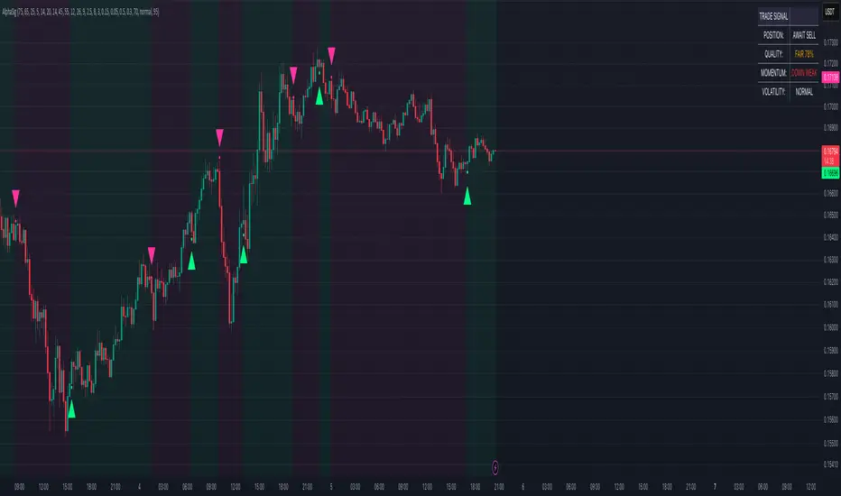
Multi-Signal Trading Indicator (MSTI)Multi-Signal Trading Indicator (MSTI)
Overview
The Multi-Signal Trading Indicator (MSTI) is a comprehensive technical analysis tool that combines eight powerful indicators into a single, unified system. Designed to identify high-probability trading opportunities, MSTI generates precise buy and sell signals by analyzing multiple market factors simultaneously. The indicator excels at detecting potential reversals and trend continuations while filtering out market noise.
Key Features
8 Core Technical Components
MACD: Identifies momentum changes and potential trend reversals
RSI: Detects overbought and oversold conditions
Bollinger Bands: Analyzes price volatility and extreme conditions
Stochastic Oscillator: Identifies potential turning points in price
Moving Averages: Confirms trend direction using dual SMAs
Volume Analysis: Validates price movements with volume confirmation
Fibonacci Levels: Identifies key support/resistance areas
Divergence Detection: Spots divergences between price and momentum
Advanced Predictive Capabilities
Volume Surge Detection: Identifies significant volume increases that often precede major price movements
Enhanced Divergence Analysis: Detects both regular and hidden divergences for early reversal signals
Support/Resistance Tests: Identifies successful tests of key support/resistance zones
Momentum Change Detection: Spots early shifts in price momentum using Rate of Change
Order Flow Analysis: Tracks buying/selling pressure through On-Balance Volume
Signal Quality Management
Adjustable Signal Thresholds: Customize the number of conditions required for signal generation
Multiple Quality Levels: Choose between Normal, High, and Maximum quality settings
Strength Measurement: Displays signal strength as a percentage for better decision-making
Repeat Signal Prevention: Eliminates duplicate signals to reduce noise
Visual Features
Clear Chart Markers: Buy/sell signals displayed directly on price chart
Comprehensive Info Panel: Shows status of all components and overall signal information
Customizable Colors: Adjust visual elements to match your chart theme
Practical Applications
For Day Traders
Identify short-term reversal points with high accuracy
Validate entries with multiple confirmations
Filter out false signals during choppy market conditions
For Swing Traders
Spot early trend changes before they become obvious
Enter positions with higher confidence and precision
Hold positions through noise by following true trend signals
For Position Traders
Identify major trend reversals with multiple confirmations
Filter out minor retracements from significant trend changes
Time entries and exits with greater precision
Customization Options
MSTI is highly customizable with over 30 adjustable parameters allowing you to:
Fine-tune each technical component
Adjust signal quality and filtering
Enable/disable specific components
Customize visual appearance
Usage Tips
Start with the Normal quality setting to understand signal frequency
Progress to High or Maximum settings for fewer but higher quality signals
Adjust minimum conditions based on market volatility
Enable trend filter in trending markets for better signal accuracy
Enable volatility filter to avoid signals during low-volatility periods