AI AAdaptive Supertrend ChannelAI Supertrend Channel – The Adaptive Trend System
Beyond Basic Supertrend: An Intelligent Trading Framework
The AI Adaptive Supertrend Channel transcends traditional trend following indicators by delivering a self-optimizing trading system. Its core innovation is a triple-adaptive engine that automatically adjusts channel width based on real-time market conditions:
Market Efficiency Detection – Widens during clean trends, tightens in choppy ranges
Normalized Volatility – Scales appropriately to any asset's price level
Dynamic Momentum Response – Expands aggressively during powerful directional moves
The Result: A smarter tool that reduces false signals in consolidation while giving trends ample room to run—eliminating the constant parameter tweaking required by static indicators.
Visual Signal Framework & Strategic Applications
Channel Architecture:
Primary Trend Line (Thick Green/Red): Your dynamic trailing stop and core trend indicator. Green signals an uptrend (buying bias), Red signals a downtrend (selling bias).
Upper & Lower Bands: Form a dynamic support/resistance channel around the trend.
Mid-Line: A critical mean reversion level and the trigger for key early signals.
Trading Signals & Strategic Meaning:
Primary Signal: Momentum Diamonds (High Conviction)
💎 Green Diamond (Higher High): Price closes above the Upper Band after making a new high. Signals strong bullish momentum continuation. Ideal for adding to long positions or entering new longs in an established uptrend.
💎 Red Diamond (Lower Low): Price closes below the Lower Band after making a new low. Signals strong bearish momentum continuation. Ideal for adding to short positions or entering new shorts in a downtrend.
Secondary Signal: Mid-Line Crosses (Early Action)
🔼 Green Triangle (Bullish Mid-Line Cross - bullMidCross): Price crosses above the Mid-Line. This is an early bullish pullback signal within a larger uptrend or a potential early reversal sign in a downtrend. Use for early entries or to confirm the end of a bearish pullback.
🔽 Red Triangle (Bearish Mid-Line Cross - bearMidCross): Price crosses below the Mid-Line. This is an early bearish pullback signal within a larger downtrend or a potential early warning of weakness in an uptrend. Use for early short entries or to take profits on longs.
Practical Trading Strategies
Trend Following: Align trades with the Primary Trend Line color. Use the line itself as a dynamic stop-loss. The Momentum Diamonds confirm the trend's strength.
Pullback Trading: Use the Mid-Line Cross triangles (bullMidCross/bearMidCross) to identify high-probability entries during trend retracements. The channel bands provide natural profit targets.
Breakout Confirmation: A Momentum Diamond following a period of consolidation often confirms a genuine breakout, offering a signal to enter with the new momentum.
Optimal Settings Guide
Default (Universal)
For most markets, timeframes
ATR: 13 | ER: 144 | Channel Width: 0.7
Volatility Factor: 100 | Vol MA: HMA | Trend MA: EMA
Day Trading (Fast, Responsive)
*15M-1H charts, scalping*
ATR: 8 | ER: 89 | Channel Width: 0.6
Volatility Factor: 120 | Vol MA: EMA | Trend MA: WMA
*Swing Trading (Smooth, Conservative)*
*Daily-Weekly, position trading*
ATR: 21 | ER: 200 | Channel Width: 0.9
Volatility Factor: 80 | Vol MA: HMA | Trend MA: LINREG
Channel Width × Factor
0.5-0.7 → Tighter (more signals, less room)
0.8-1.2 → Wider (fewer signals, more room to run)
Volatility Regime Factor
50-80 → Less sensitive to volatility (stable markets)
100-150 → More sensitive (volatile markets like crypto)
Base ATR Length
8-13 → Faster signals (lower timeframes)
17-21 → Smoother signals (higher timeframes)
Quick Adjustments:
Whipsaws → Increase Channel Width × Factor
Lagging → Decrease ATR Length
Volatile markets → Increase Volatility Regime Factor
Start with Default, adjust one parameter at a time based on your market and trading style.
Search in scripts for "ai"

AI Trend Navigator [K-Neighbor]█ Overview
In the evolving landscape of trading and investment, the demand for sophisticated and reliable tools is ever-growing. The AI Trend Navigator is an indicator designed to meet this demand, providing valuable insights into market trends and potential future price movements. The AI Trend Navigator indicator is designed to predict market trends using the k-Nearest Neighbors (KNN) classifier.
By intelligently analyzing recent price actions and emphasizing similar values, it helps traders to navigate complex market conditions with confidence. It provides an advanced way to analyze trends, offering potentially more accurate predictions compared to simpler trend-following methods.
█ Calculations
KNN Moving Average Calculation: The core of the algorithm is a KNN Moving Average that computes the mean of the 'k' closest values to a target within a specified window size. It does this by iterating through the window, calculating the absolute differences between the target and each value, and then finding the mean of the closest values. The target and value are selected based on user preferences (e.g., using the VWAP or Volatility as a target).
KNN Classifier Function: This function applies the k-nearest neighbor algorithm to classify the price action into positive, negative, or neutral trends. It looks at the nearest 'k' bars, calculates the Euclidean distance between them, and categorizes them based on the relative movement. It then returns the prediction based on the highest count of positive, negative, or neutral categories.
█ How to use
Traders can use this indicator to identify potential trend directions in different markets.
Spotting Trends: Traders can use the KNN Moving Average to identify the underlying trend of an asset. By focusing on the k closest values, this component of the indicator offers a clearer view of the trend direction, filtering out market noise.
Trend Confirmation: The KNN Classifier component can confirm existing trends by predicting the future price direction. By aligning predictions with current trends, traders can gain more confidence in their trading decisions.
█ Settings
PriceValue: This determines the type of price input used for distance calculation in the KNN algorithm.
hl2: Uses the average of the high and low prices.
VWAP: Uses the Volume Weighted Average Price.
VWAP: Uses the Volume Weighted Average Price.
Effect: Changing this input will modify the reference values used in the KNN classification, potentially altering the predictions.
TargetValue: This sets the target variable that the KNN classification will attempt to predict.
Price Action: Uses the moving average of the closing price.
VWAP: Uses the Volume Weighted Average Price.
Volatility: Uses the Average True Range (ATR).
Effect: Selecting different targets will affect what the KNN is trying to predict, altering the nature and intent of the predictions.
Number of Closest Values: Defines how many closest values will be considered when calculating the mean for the KNN Moving Average.
Effect: Increasing this value makes the algorithm consider more nearest neighbors, smoothing the indicator and potentially making it less reactive. Decreasing this value may make the indicator more sensitive but possibly more prone to noise.
Neighbors: This sets the number of neighbors that will be considered for the KNN Classifier part of the algorithm.
Effect: Adjusting the number of neighbors affects the sensitivity and smoothness of the KNN classifier.
Smoothing Period: Defines the smoothing period for the moving average used in the KNN classifier.
Effect: Increasing this value would make the KNN Moving Average smoother, potentially reducing noise. Decreasing it would make the indicator more reactive but possibly more prone to false signals.
█ What is K-Nearest Neighbors (K-NN) algorithm?
At its core, the K-NN algorithm recognizes patterns within market data and analyzes the relationships and similarities between data points. By considering the 'K' most similar instances (or neighbors) within a dataset, it predicts future price movements based on historical trends. The K-Nearest Neighbors (K-NN) algorithm is a type of instance-based or non-generalizing learning. While K-NN is considered a relatively simple machine-learning technique, it falls under the AI umbrella.
We can classify the K-Nearest Neighbors (K-NN) algorithm as a form of artificial intelligence (AI), and here's why:
Machine Learning Component: K-NN is a type of machine learning algorithm, and machine learning is a subset of AI. Machine learning is about building algorithms that allow computers to learn from and make predictions or decisions based on data. Since K-NN falls under this category, it is aligned with the principles of AI.
Instance-Based Learning: K-NN is an instance-based learning algorithm. This means that it makes decisions based on the entire training dataset rather than deriving a discriminative function from the dataset. It looks at the 'K' most similar instances (neighbors) when making a prediction, hence adapting to new information if the dataset changes. This adaptability is a hallmark of intelligent systems.
Pattern Recognition: The core of K-NN's functionality is recognizing patterns within data. It identifies relationships and similarities between data points, something akin to human pattern recognition, a key aspect of intelligence.
Classification and Regression: K-NN can be used for both classification and regression tasks, two fundamental problems in machine learning and AI. The indicator code is used for trend classification, a predictive task that aligns with the goals of AI.
Simplicity Doesn't Exclude AI: While K-NN is often considered a simpler algorithm compared to deep learning models, simplicity does not exclude something from being AI. Many AI systems are built on simple rules and can be combined or scaled to create complex behavior.
No Explicit Model Building: Unlike traditional statistical methods, K-NN does not build an explicit model during training. Instead, it waits until a prediction is required and then looks at the 'K' nearest neighbors from the training data to make that prediction. This lazy learning approach is another aspect of machine learning, part of the broader AI field.
-----------------
Disclaimer
The information contained in my Scripts/Indicators/Ideas/Algos/Systems does not constitute financial advice or a solicitation to buy or sell any securities of any type. I will not accept liability for any loss or damage, including without limitation any loss of profit, which may arise directly or indirectly from the use of or reliance on such information.
All investments involve risk, and the past performance of a security, industry, sector, market, financial product, trading strategy, backtest, or individual's trading does not guarantee future results or returns. Investors are fully responsible for any investment decisions they make. Such decisions should be based solely on an evaluation of their financial circumstances, investment objectives, risk tolerance, and liquidity needs.
My Scripts/Indicators/Ideas/Algos/Systems are only for educational purposes!

AI-Weighted RSI (Zeiierman)█ Overview
AI-Weighted RSI (Zeiierman) is an adaptive oscillator that enhances classic RSI by applying a correlation-weighted prediction layer. Instead of looking only at RSI values directly, this indicator continuously evaluates how other price- and volume-based features (returns, volatility, volume shifts) correlate with RSI, and then weights them accordingly to project the next RSI state.
The result is a smoother, forward-looking RSI framework that adapts to market conditions in real time.
By leveraging feature correlation instead of static formulas, AI-Weighted RSI behaves like a lightweight learning model, adjusting its emphasis depending on which features are most aligned with RSI behavior during the current regime.
█ How It Works
⚪ Feature Extraction
Each bar, the script computes features: log returns, RSI itself, ATR% (volatility), volume, and volume log-change.
⚪ Correlation Screening
Over a rolling learning window, it measures the correlation of each feature against RSI. The strongest relationships are ranked and selected.
⚪ Adaptive Weighting
Features are standardized (z-scored), then combined using their signed correlations as weights, building a rolling, adaptive prediction of RSI.
⚪ Prediction to RSI Weight
The predicted RSI is mapped back into a “weight” scale (±2 by default). Above 0 = bullish bias, below 0 = bearish bias, with color-graded fills to visualize overbought/oversold pressure.
⚪ Signal Line
A smoothing option (signal length) overlays a moving average of the AI-Weighted RSI for clearer trend confirmation.
█ Why AI-Weighted RSI
⚪ Adaptive to Market Regime
Because the model re-evaluates correlations continuously, it naturally shifts which features dominate, sometimes volatility explains RSI best, sometimes volume, sometimes returns.
⚪ Forward-Looking Bias
Instead of simply reflecting RSI, the model provides a projection, helping anticipate shifts in momentum before RSI itself flips.
█ How to Use
⚪ Directional Bias
Read the RSI relative to 0. Above = bullish momentum bias, below = bearish.
⚪ Overbought / Oversold Zones
Shaded fills beyond +0.5 or -0.5 highlight extremes where RSI pressure often exhausts.
⚪ Divergences
When price makes new highs/lows but AI-Weighted RSI fails to confirm, it often signals weakening momentum.
█ Settings
RSI Length: Lookback for the core RSI calculation.
Signal Length: Smoothing applied to the AI-Weighted RSI output.
Learning Window: Bars used for correlation learning and z-scoring.
-----------------
Disclaimer
The content provided in my scripts, indicators, ideas, algorithms, and systems is for educational and informational purposes only. It does not constitute financial advice, investment recommendations, or a solicitation to buy or sell any financial instruments. I will not accept liability for any loss or damage, including without limitation any loss of profit, which may arise directly or indirectly from the use of or reliance on such information.
All investments involve risk, and the past performance of a security, industry, sector, market, financial product, trading strategy, backtest, or individual's trading does not guarantee future results or returns. Investors are fully responsible for any investment decisions they make. Such decisions should be based solely on an evaluation of their financial circumstances, investment objectives, risk tolerance, and liquidity needs.

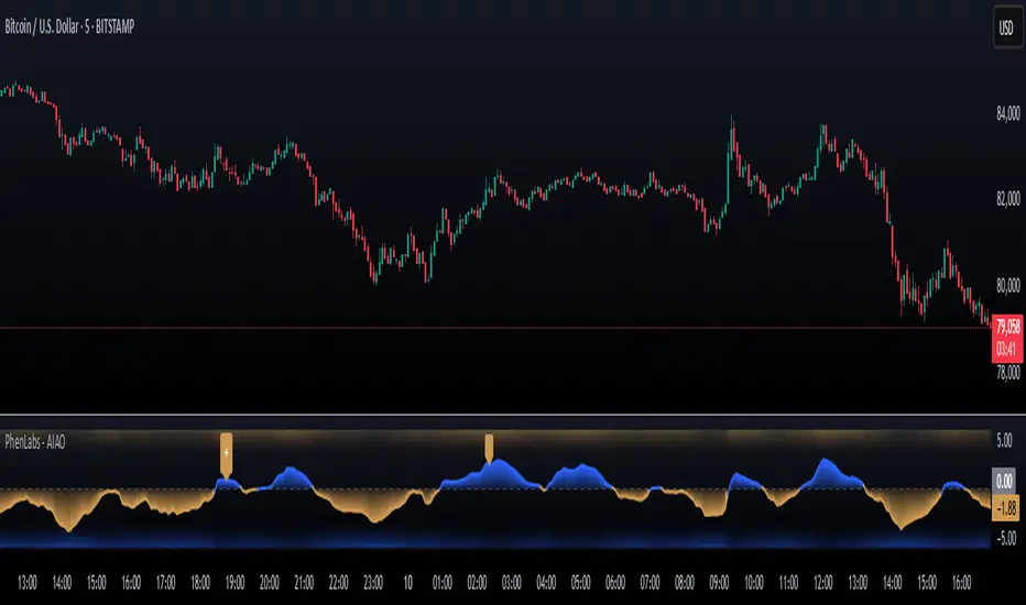
AI Adaptive Oscillator [PhenLabs]📊 Algorithmic Adaptive Oscillator
Version: PineScript™ v6
📌 Description
The AI Adaptive Oscillator is a sophisticated technical indicator that employs ensemble learning and adaptive weighting techniques to analyze market conditions. This innovative oscillator combines multiple traditional technical indicators through an AI-driven approach that continuously evaluates and adjusts component weights based on historical performance. By integrating statistical modeling with machine learning principles, the indicator adapts to changing market dynamics, providing traders with a responsive and reliable tool for market analysis.
🚀 Points of Innovation:
Ensemble learning framework with adaptive component weighting
Performance-based scoring system using directional accuracy
Dynamic volatility-adjusted smoothing mechanism
Intelligent signal filtering with cooldown and magnitude requirements
Signal confidence levels based on multi-factor analysis
🔧 Core Components
Ensemble Framework : Combines up to five technical indicators with performance-weighted integration
Adaptive Weighting : Continuous performance evaluation with automated weight adjustment
Volatility-Based Smoothing : Adapts sensitivity based on current market volatility
Pattern Recognition : Identifies potential reversal patterns with signal qualification criteria
Dynamic Visualization : Professional color schemes with gradient intensity representation
Signal Confidence : Three-tiered confidence assessment for trading signals
🔥 Key Features
The indicator provides comprehensive market analysis through:
Multi-Component Ensemble : Integrates RSI, CCI, Stochastic, MACD, and Volume-weighted momentum
Performance Scoring : Evaluates each component based on directional prediction accuracy
Adaptive Smoothing : Automatically adjusts based on market volatility
Pattern Detection : Identifies potential reversal patterns in overbought/oversold conditions
Signal Filtering : Prevents excessive signals through cooldown periods and minimum change requirements
Confidence Assessment : Displays signal strength through intuitive confidence indicators (average, above average, excellent)
🎨 Visualization
Gradient-Filled Oscillator : Color intensity reflects strength of market movement
Clear Signal Markers : Distinct bullish and bearish pattern signals with confidence indicators
Range Visualization : Clean representation of oscillator values from -6 to 6
Zero Line : Clear demarcation between bullish and bearish territory
Customizable Colors : Color schemes that can be adjusted to match your chart style
Confidence Symbols : Intuitive display of signal confidence (no symbol, +, or ++) alongside direction markers
📖 Usage Guidelines
⚙️ Settings Guide
Color Settings
Bullish Color
Default: #2b62fa (Blue)
This setting controls the color representation for bullish movements in the oscillator. The color appears when the oscillator value is positive (above zero), with intensity indicating the strength of the bullish momentum. A brighter shade indicates stronger bullish pressure.
Bearish Color
Default: #ce9851 (Amber)
This setting determines the color representation for bearish movements in the oscillator. The color appears when the oscillator value is negative (below zero), with intensity reflecting the strength of the bearish momentum. A more saturated shade indicates stronger bearish pressure.
Signal Settings
Signal Cooldown (bars)
Default: 10
Range: 1-50
This parameter sets the minimum number of bars that must pass before a new signal of the same type can be generated. Higher values reduce signal frequency and help prevent overtrading during choppy market conditions. Lower values increase signal sensitivity but may generate more false positives.
Min Change For New Signal
Default: 1.5
Range: 0.5-3.0
This setting defines the minimum required change in oscillator value between consecutive signals of the same type. It ensures that new signals represent meaningful changes in market conditions rather than minor fluctuations. Higher values produce fewer but potentially higher-quality signals, while lower values increase signal frequency.
AI Core Settings
Base Length
Default: 14
Minimum: 2
This fundamental setting determines the primary calculation period for all technical components in the ensemble (RSI, CCI, Stochastic, etc.). It represents the lookback window for each component’s base calculation. Shorter periods create a more responsive but potentially noisier oscillator, while longer periods produce smoother signals with potential lag.
Adaptive Speed
Default: 0.1
Range: 0.01-0.3
Controls how quickly the oscillator adapts to new market conditions through its volatility-adjusted smoothing mechanism. Higher values make the oscillator more responsive to recent price action but potentially more erratic. Lower values create smoother transitions but may lag during rapid market changes. This parameter directly influences the indicator’s adaptiveness to market volatility.
Learning Lookback Period
Default: 150
Minimum: 10
Determines the historical data range used to evaluate each ensemble component’s performance and calculate adaptive weights. This setting controls how far back the AI “learns” from past performance to optimize current signals. Longer periods provide more stable weight distribution but may be slower to adapt to regime changes. Shorter periods adapt more quickly but may overreact to recent anomalies.
Ensemble Size
Default: 5
Range: 2-5
Specifies how many technical components to include in the ensemble calculation.
Understanding The Interaction Between Settings
Base Length and Learning Lookback : The base length determines the reactivity of individual components, while the lookback period determines how their weights are adjusted. These should be balanced according to your timeframe - shorter timeframes benefit from shorter base lengths, while the lookback should generally be 10-15 times the base length for optimal learning.
Adaptive Speed and Signal Cooldown : These settings control sensitivity from different angles. Increasing adaptive speed makes the oscillator more responsive, while reducing signal cooldown increases signal frequency. For conservative trading, keep adaptive speed low and cooldown high; for aggressive trading, do the opposite.
Ensemble Size and Min Change : Larger ensembles provide more stable signals, allowing for a lower minimum change threshold. Smaller ensembles might benefit from a higher threshold to filter out noise.
Understanding Signal Confidence Levels
The indicator provides three distinct confidence levels for both bullish and bearish signals:
Average Confidence (▲ or ▼) : Basic signal that meets the minimum pattern and filtering criteria. These signals indicate potential reversals but with moderate confidence in the prediction. Consider using these as initial alerts that may require additional confirmation.
Above Average Confidence (▲+ or ▼+) : Higher reliability signal with stronger underlying metrics. These signals demonstrate greater consensus among the ensemble components and/or stronger historical performance. They offer increased probability of successful reversals and can be traded with less additional confirmation.
Excellent Confidence (▲++ or ▼++) : Highest quality signals with exceptional underlying metrics. These signals show strong agreement across oscillator components, excellent historical performance, and optimal signal strength. These represent the indicator’s highest conviction trade opportunities and can be prioritized in your trading decisions.
Confidence assessment is calculated through a multi-factor analysis including:
Historical performance of ensemble components
Degree of agreement between different oscillator components
Relative strength of the signal compared to historical thresholds
✅ Best Use Cases:
Identify potential market reversals through oscillator extremes
Filter trade signals based on AI-evaluated component weights
Monitor changing market conditions through oscillator direction and intensity
Confirm trade signals from other indicators with adaptive ensemble validation
Detect early momentum shifts through pattern recognition
Prioritize trading opportunities based on signal confidence levels
Adjust position sizing according to signal confidence (larger for ++ signals, smaller for standard signals)
⚠️ Limitations
Requires sufficient historical data for accurate performance scoring
Ensemble weights may lag during dramatic market condition changes
Higher ensemble sizes require more computational resources
Performance evaluation quality depends on the learning lookback period length
Even high confidence signals should be considered within broader market context
💡 What Makes This Unique
Adaptive Intelligence : Continuously adjusts component weights based on actual performance
Ensemble Methodology : Combines strength of multiple indicators while minimizing individual weaknesses
Volatility-Adjusted Smoothing : Provides appropriate sensitivity across different market conditions
Performance-Based Learning : Utilizes historical accuracy to improve future predictions
Intelligent Signal Filtering : Reduces noise and false signals through sophisticated filtering criteria
Multi-Level Confidence Assessment : Delivers nuanced signal quality information for optimized trading decisions
🔬 How It Works
The indicator processes market data through five main components:
Ensemble Component Calculation :
Normalizes traditional indicators to consistent scale
Includes RSI, CCI, Stochastic, MACD, and volume components
Adapts based on the selected ensemble size
Performance Evaluation :
Analyzes directional accuracy of each component
Calculates continuous performance scores
Determines adaptive component weights
Oscillator Integration :
Combines weighted components into unified oscillator
Applies volatility-based adaptive smoothing
Scales final values to -6 to 6 range
Signal Generation :
Detects potential reversal patterns
Applies cooldown and magnitude filters
Generates clear visual markers for qualified signals
Confidence Assessment :
Evaluates component agreement, historical accuracy, and signal strength
Classifies signals into three confidence tiers (average, above average, excellent)
Displays intuitive confidence indicators (no symbol, +, ++) alongside direction markers
💡 Note:
The AI Adaptive Oscillator performs optimally when used with appropriate timeframe selection and complementary indicators. Its adaptive nature makes it particularly valuable during changing market conditions, where traditional fixed-weight indicators often lose effectiveness. The ensemble approach provides a more robust analysis by leveraging the collective intelligence of multiple technical methodologies. Pay special attention to the signal confidence indicators to optimize your trading decisions - excellent (++) signals often represent the most reliable trade opportunities.
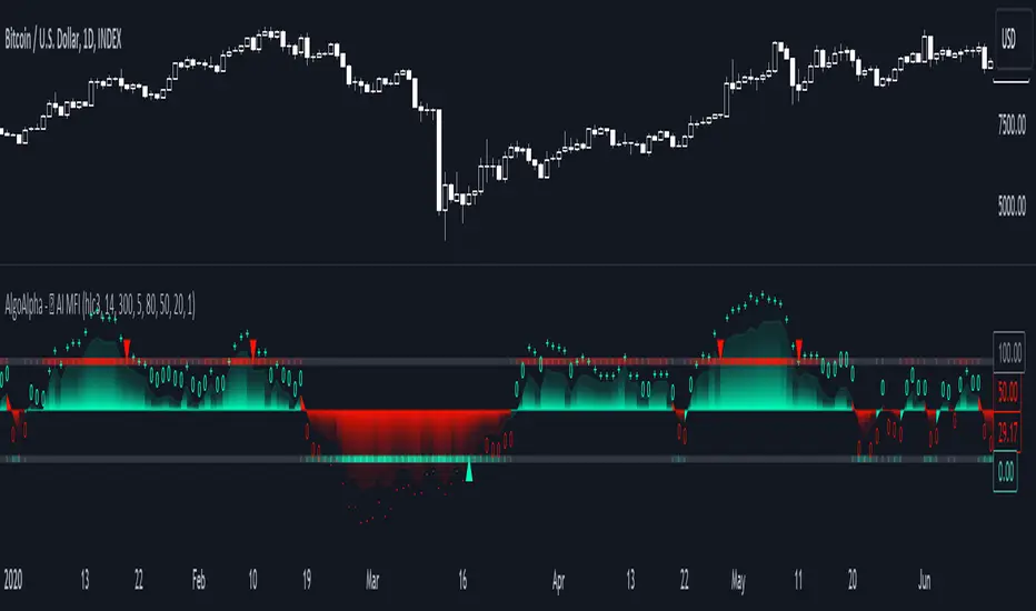
AI Adaptive Money Flow Index (Clustering) [AlgoAlpha]🌟🚀 Dive into the future of trading with our latest innovation: the AI Adaptive Money Flow Index by AlgoAlpha Indicator! 🚀🌟
Developed with the cutting-edge power of Machine Learning, this indicator is designed to revolutionize the way you view market dynamics. 🤖💹 With its unique blend of traditional Money Flow Index (MFI) analysis and advanced k-means clustering, it adapts to market conditions like never before.
Key Features:
📊 Adaptive MFI Analysis: Utilizes the classic MFI formula with a twist, adjusting its parameters based on AI-driven clustering.
🧠 AI-Driven Clustering: Applies k-means clustering to identify and adapt to market states, optimizing the MFI for current conditions.
🎨 Customizable Appearance: Offers adjustable settings for overbought, neutral, and oversold levels, as well as colors for uptrends and downtrends.
🔔 Alerts for Key Market Movements: Set alerts for trend reversals, overbought, and oversold conditions, ensuring you never miss a trading opportunity.
Quick Guide to Using the AI Adaptive MFI (Clustering):
🛠 Customize the Indicator: Customize settings like MFI source, length, and k-means clustering parameters to suit your analysis.
📈 Market Analysis: Monitor the dynamically adjusted overbought, neutral, and oversold levels for insights into market conditions. Watch for classification symbols ("+", "0", "-") for immediate understanding of the current market state. Look out for reversal signals (▲, ▼) to get potential entry points.
🔔 Set Alerts: Utilize the built-in alert conditions for trend changes, overbought, and oversold signals to stay ahead, even when you're not actively monitoring the charts.
How It Works:
The AI Adaptive Money Flow Index employs the k-means clustering machine learning algorithm to refine the traditional Money Flow Index, dynamically adjusting overbought, neutral, and oversold levels based on market conditions. This method analyzes historical MFI values, grouping them into initial clusters using the traditional MFI's overbought, oversold and neutral levels, and then finding the mean of each cluster, which represent the new market states thresholds. This adaptive approach ensures the indicator's sensitivity in real-time, offering a nuanced understanding of market trend and volume analysis.
By recalibrating MFI thresholds for each new data bar, the AI Adaptive MFI intelligently conforms to changing market dynamics. This process, assessing past periods to adjust the indicator's parameters, provides traders with insights finely tuned to recent market behavior. Such innovation enhances decision-making, leveraging the latest data to inform trading strategies. 🌐💥
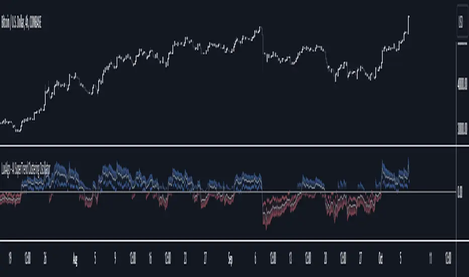
AI SuperTrend Clustering Oscillator [LuxAlgo]The AI SuperTrend Clustering Oscillator is an oscillator returning the most bullish/average/bearish centroids given by multiple instances of the difference between SuperTrend indicators.
This script is an extension of our previously posted SuperTrend AI indicator that makes use of k-means clustering. If you want to learn more about it see:
🔶 USAGE
The AI SuperTrend Clustering Oscillator is made of 3 distinct components, a bullish output (always the highest), a bearish output (always the lowest), and a "consensus" output always within the two others.
The general trend is given by the consensus output, with a value above 0 indicating an uptrend and under 0 indicating a downtrend. Using a higher minimum factor will weigh results toward longer-term trends, while lowering the maximum factor will weigh results toward shorter-term trends.
Strong trends are indicated when the bullish/bearish outputs are indicating an opposite sentiment. A strong bullish trend would for example be indicated when the bearish output is above 0, while a strong bearish trend would be indicated when the bullish output is below 0.
When the consensus output is indicating a specific trend direction, an opposite indication from the bullish/bearish output can highlight a potential reversal or retracement.
🔶 DETAILS
The indicator construction is based on finding three clusters from the difference between the closing price and various SuperTrend using different factors. The centroid of each cluster is then returned. This operation is done over all historical bars.
The highest cluster will be composed of the differences between the price and SuperTrends that are the highest, thus creating a more bullish group. The lowest cluster will be composed of the differences between the price and SuperTrends that are the lowest, thus creating a more bearish group.
The consensus cluster is composed of the differences between the price and SuperTrends that are not significant enough to be part of the other clusters.
🔶 SETTINGS
ATR Length: ATR period used for the calculation of the SuperTrends.
Factor Range: Determine the minimum and maximum factor values for the calculation of the SuperTrends.
Step: Increments of the factor range.
Smooth: Degree of smoothness of each output from the indicator.
🔹 Optimization
This group of settings affects the runtime performances of the script.
Maximum Iteration Steps: Maximum number of iterations allowed for finding centroids. Excessively low values can return a better script load time but poor clustering.
Historical Bars Calculation: Calculation window of the script (in bars).
AI Chakra for Global Markets by Pooja🌐 AI Chakra for Global Markets by Pooja
⚡ Advanced Multi-Signal Trading Framework for Forex & Crypto
AI Chakra is a complete institutional-grade market analysis system, combining
Trend + Structure + Momentum + Volatility + Breakouts + Multi-TF Context + Smart Levels
into a single clean and powerful charting tool.
Designed especially for Forex and Crypto, where speed, precision and clarity matter most.
✨ Key Features
1️⃣ 🎯 Smart Auto Buy/Sell Signal System
Signals appear only when multiple conditions align:
✔️ Buy Sell Signals include:
🟢 Supertrend in bullish zone
💪 RSI momentum in upper strength zone
🔄 CHoCH or BOS supporting upward shift
🚀 Breakout above key levels (Prev-Day High)
⚙️ Optional filters: ADX-Volatility + RSI-MA Protection
✔️ Sell Signals include:
🔴 Supertrend bearish
📉 RSI in weakness zone
🔄 CHoCH/BOS supporting downward structure
🕳️ Breakout below previous-day low
⚙️ Optional filters for momentum validation
📌 Signals are printed as clean labels — visually distinct and easy to interpret.
2️⃣ 🧠 Smart Money Concepts (SMC Suite)
Built-in structural analysis for professional traders:
🔶 CHoCH (Change of Character)
🔷 BOS (Break of Structure)
Every CHoCH/BOS is plotted with:
Horizontal structural level
Precision labels
ATR-adjusted spacing to avoid overlap
Perfect for identifying:
✔️ Trend reversals
✔️ Continuation breaks
✔️ Manipulation zones
✔️ Smart entry areas
3️⃣ 📊 Multi-Timeframe Trend Dashboard (Top-Down View)
A clean institutional-level dashboard across:
1m ▸ 5m ▸ 15m ▸ 30m ▸ 1H ▸ 4H ▸ 1D ▸ 1W ▸ 1M
Each timeframe evaluates:
EMA alignment
VWAP alignment
Supertrend direction
Shows 🔵 Bullish, 🔴 Bearish, ⚪ Neutral
in a visually intuitive format.
4️⃣ 📐 Auto Trendline System + Breakout Detection (Optional Module)
When enabled:
Detects swing highs/lows automatically
Draws dynamic support/resistance trendlines
Uses ATR / Stdev / Linear Regression slopes
Extends lines into future
Marks Breakout events with labels
Ideal for:
✔️ Crypto volatility
✔️ Forex swings
✔️ Breakout traders
✔️ Channel/wedge detection
5️⃣ 🏛️ Institutional Levels – Traditional Pivot Points
Includes complete dynamic Support/Resistance map:
Daily / Weekly / Monthly
Quarterly / Yearly
Multi-Year levels
Adjustable:
Line width
Line color
Price labels (Left/Right)
Works perfectly for:
XAUUSD
GBPJPY
EURUSD
BTCUSDT
NAS100
US30
📌 6. Volatility & Momentum Safety Filters (Optional)
ADX Filter
Allows signals only when volatility/trend strength is acceptable
Avoids signals in low-volatility sideways markets
RSI-MA Filter
Detects fake breakouts
Evaluates RSI displacement & momentum slope
Keeps only reliable directional conditions
These filters help refine signals for Forex (high-flow sessions) and Crypto (high-volatility assets).
📌 7. Previous-Day High/Low Break Detection
A pure price-action breakout feature tuned for global markets:
Detects clean breaks of yesterday’s high (bullish strength)
Detects breaks of yesterday’s low (bearish weakness)
Auto-avoids duplicate prints
Works extremely well in:
XAUUSD
GBPJPY
BTCUSDT
ETHUSDT
Indices like NAS100 or US30
6️⃣ 📡 JSON-Ready Alerts (Webhook Compatible)
Send signals directly to:
Telegram bots
Discord servers
Custom trading bots
Automation platforms
Every Buy/Sell alert includes JSON payload support.
🌍 Optimized for Global Markets
Forex
EURUSD • GBPJPY • XAUUSD • USDJPY • GBPUSD • AUDUSD
Majors, minors, exotics supported.
Crypto
BTC • ETH • SOL • BNB • XRP • Futures & Spot.
Timeframes Supported
Scalping: 1m–15m
Intraday: 30m–4H
Swing: 1D–1W–1M
⚠️ Policy-Safe Disclaimer
This script is a technical analysis tool, not financial advice.
It does not guarantee profits or automate trading decisions.
Always verify signals with your own strategy and risk management.
🌟 Final Summary
AI Chakra unifies:
📈 Trend
🧠 Structure
🎯 Signals
💹 Momentum
🔥 Breakouts
🏛️ Institutional Levels
🧩 Multi-TF Logic
🔐 ACCESS
This version is an Invite-Only Script.
Access is granted manually.
🛡 Support
This is an invite-only indicator.
Approved users may contact the author via the “Author’s Instructions” section on TradingView for help or usage guidance.

AI Breakout Bands (Zeiierman)█ Overview
AI Breakout Bands (Zeiierman) is an adaptive trend and breakout detection system that combines Kalman filtering with advanced K-Nearest Neighbor (KNN) smoothing. The result is a smart, self-adjusting band structure that adapts to dynamic market behavior, identifying breakout conditions with precision and visual clarity.
At its core, this indicator estimates price behavior using a two-dimensional Kalman filter (position + velocity), then enhances the smoothing process with a nonlinear, similarity-based KNN filter. This unique blend enables it to handle noisy markets and directional shifts with both speed and stability — providing breakout traders and trend followers a reliable framework to act on.
Whether you're identifying volatility expansions, capturing trend continuations, or spotting early breakout conditions, AI Breakout Bands gives you a mathematically grounded, visually adaptive roadmap of real-time market structure.
█ How It Works
⚪ Kalman Filter Engine
The Kalman filter models price movement as a state system with two components:
Position (price)
Velocity (trend direction)
It recursively updates predictions using real-time price as a noisy observation, balancing responsiveness with smoothness.
Process Noise (Position) controls sensitivity to sudden moves.
Process Noise (Velocity) controls smoothing of directional flow.
Measurement Noise (R) defines how much the filter "trusts" live price data.
This component alone creates a responsive yet stable estimate of the market’s center of gravity.
⚪ Advanced K-Neighbor Smoothing
After the Kalman estimate is computed, the script applies a custom K-Nearest Neighbor (KNN) smoother.
Rather than averaging raw values, this method:
Finds K most similar past Kalman values
Weighs them by similarity (inverse of absolute distance)
Produces a smoother that emphasizes structural similarity
This nonlinear approach gives the indicator an AI feature — reacting fast when needed, yet staying calm in consolidation.
█ How to Use
⚪ Trend Recognition
The line color shifts dynamically based on slope direction and breakout confirmation.
Bullish conditions: price above the mid band with positive slope
Bearish conditions: price below the mid band with negative slope
⚪ Breakout Signals
Price breaking above or below the bands may signal momentum acceleration.
Combine with your own volume or momentum confirmation for stronger entries.
Bands adapt to market noise, helping filter out low-quality whipsaws.
█ Settings
Process Noise (Position): Controls Kalman filter’s sensitivity to price changes.
Process Noise (Velocity): Controls smoothing of directional component.
Measurement Noise (R): Defines how much trust is placed in price data.
K-Neighbor Length: Number of historical Kalman values considered for smoothing.
Slope Calculation Window: Number of bars used to compute trend slope of the smoothed Kalman.
Band Lookback (MAE): Rolling period for average absolute error.
Band Multiplier: Multiplies MAE to determine band width.
-----------------
Disclaimer
The content provided in my scripts, indicators, ideas, algorithms, and systems is for educational and informational purposes only. It does not constitute financial advice, investment recommendations, or a solicitation to buy or sell any financial instruments. I will not accept liability for any loss or damage, including without limitation any loss of profit, which may arise directly or indirectly from the use of or reliance on such information.
All investments involve risk, and the past performance of a security, industry, sector, market, financial product, trading strategy, backtest, or individual's trading does not guarantee future results or returns. Investors are fully responsible for any investment decisions they make. Such decisions should be based solely on an evaluation of their financial circumstances, investment objectives, risk tolerance, and liquidity needs.

AI Volume Breakout for scalpingPurpose of the Indicator
This script is designed for trading, specifically for scalping, which involves making numerous trades within a very short time frame to take advantage of small price movements. The indicator looks for volume breakouts, which are moments when trading volume significantly increases, potentially signaling the start of a new price movement.
Key Components:
Parameters:
Volume Threshold (volumeThreshold): Determines how much volume must increase from one bar to the next for it to be considered significant. Set at 4.0, meaning volume must quadruplicate for a breakout signal.
Price Change Threshold (priceChangeThreshold): Defines the minimum price change required for a breakout signal. Here, it's 1.5% of the bar's opening price.
SMA Length (smaLength): The period for the Simple Moving Average, which helps confirm the trend direction. Here, it's set to 20.
Cooldown Period (cooldownPeriod): Prevents signals from being too close together, set to 10 bars.
ATR Period (atrPeriod): The period for calculating Average True Range (ATR), used to measure market volatility.
Volatility Threshold (volatilityThreshold): If ATR divided by the close price exceeds this, the market is considered too volatile for trading according to this strategy.
Calculations:
SMA (Simple Moving Average): Used for trend confirmation. A bullish signal is more likely if the price is above this average.
ATR (Average True Range): Measures market volatility. Lower volatility (below the threshold) is preferred for this strategy.
Signal Generation:
The indicator checks if:
Volume has increased significantly (volumeDelta > 0 and volume / volume >= volumeThreshold).
There's enough price change (math.abs(priceDelta / open) >= priceChangeThreshold).
The market isn't too volatile (lowVolatility).
The trend supports the direction of the price change (trendUp for bullish, trendDown for bearish).
If all these conditions are met, it predicts:
1 (Bullish) if conditions suggest buying.
0 (Bearish) if conditions suggest selling.
Cooldown Mechanism:
After a signal, the script waits for a number of bars (cooldownPeriod) before considering another signal to avoid over-trading.
Visual Feedback:
Labels are placed on the chart:
Green label for bullish breakouts below the low price.
Red label for bearish breakouts above the high price.
How to Use:
Entry Points: Look for the labels on your chart to decide when to enter trades.
Risk Management: Since this is for scalping, ensure each trade has tight stop-losses to manage risk due to the quick, small movements.
Market Conditions: This strategy might work best in markets with consistent volume and price changes but not extreme volatility.
Caveats:
This isn't real AI; it's a heuristic based on volume and price. Actual AI would involve machine learning algorithms trained on historical data.
Always backtest any strategy, and consider how it behaves in different market conditions, not just the ones it was designed for.

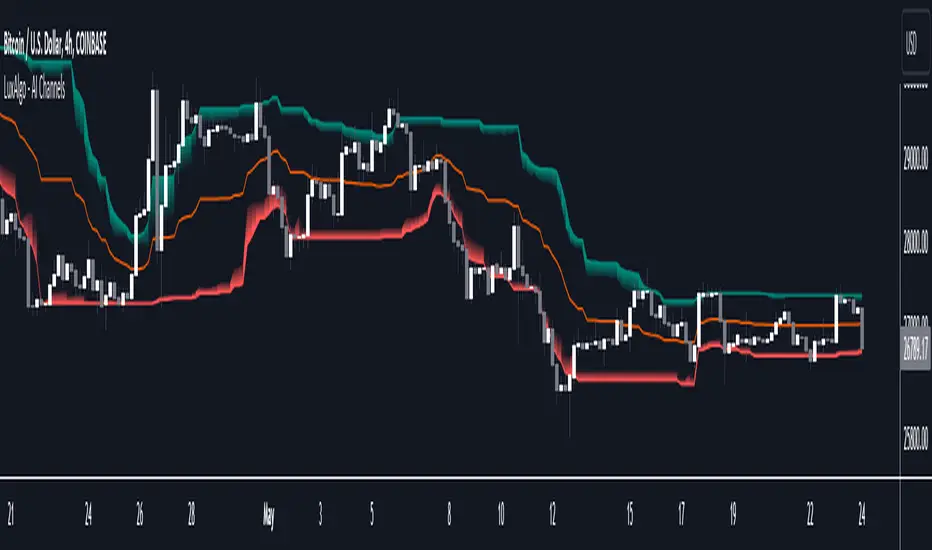
AI Channels (Clustering) [LuxAlgo]The AI Channels indicator is constructed based on rolling K-means clustering, a common machine learning method used for clustering analysis. These channels allow users to determine the direction of the underlying trends in the price.
We also included an option to display the indicator as a trailing stop from within the settings.
🔶 USAGE
Each channel extremity allows users to determine the current trend direction. Price breaking over the upper extremity suggesting an uptrend, and price breaking below the lower extremity suggesting a downtrend. Using a higher Window Size value will return longer-term indications.
The "Clusters" setting allows users to control how easy it is for the price to break an extremity, with higher values returning extremities further away from the price.
The "Denoise Channels" is enabled by default and allows to see less noisy extremities that are more coherent with the detected trend.
Users who wish to have more focus on a detected trend can display the indicator as a trailing stop.
🔹 Centroid Dispersion Areas
Each extremity is made of one area. The width of each area indicates how spread values within a cluster are around their centroids. A wider area would suggest that prices within a cluster are more spread out around their centroid, as such one could say that it is indicative of the volatility of a cluster.
Wider areas around a specific extremity can indicate a larger and more spread-out amount of prices within the associated cluster. In practice price entering an area has a higher chance to break an associated extremity.
🔶 DETAILS
The indicator performs K-means clustering over the most recent Window Size prices, finding a number of user-specified clusters. See here to find more information on cluster detection.
The channel extremities are returned as the centroid of the lowest, average, and highest price clusters.
K-means clustering can be computationally expensive and as such we allow users to determine the maximum number of iterations used to find the centroids as well as the number of most historical bars to perform the indicator calculation. Do note that increasing the calculation window of the indicator as well as the number of clusters will return slower results.
🔶 SETTINGS
Window Size: Amount of most recent prices to use for the calculation of the indicator.
Clusters": Amount of clusters detected for the calculation of the indicator.
Denoise Channels: When enabled, return less noisy channels extremities, disabling this setting will return the exact centroids at each time but will produce less regular extremities.
As Trailing Stop: Display the indicator as a trailing stop.
🔹 Optimization
This group of settings affects the runtime performance of the script.
Maximum Iteration Steps: Maximum number of iterations allowed for finding centroids. Excessively low values can return a better script load time but poor clustering.
Historical Bars Calculation: Calculation window of the script (in bars).
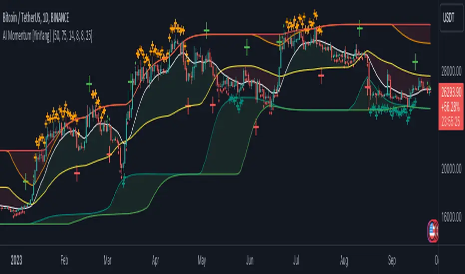
AI Momentum [YinYang]Overview:
AI Momentum is a kernel function based momentum Indicator. It uses Rational Quadratics to help smooth out the Moving Averages, this may give them a more accurate result. This Indicator has 2 main uses, first it displays ‘Zones’ that help you visualize the potential movement areas and when the price is out of bounds (Overvalued or Undervalued). Secondly it creates signals that display the momentum of the current trend.
The Zones are composed of the Highest Highs and Lowest lows turned into a Rational Quadratic over varying lengths. These create our Rational High and Low zones. There is however a second zone. The second zone is composed of the avg of the Inner High and Inner Low zones (yellow line) and the Rational Quadratic of the current Close. This helps to create a second zone that is within the High and Low bounds that may represent momentum changes within these zones. When the Rationalized Close crosses above the High and Low Zone Average it may signify a bullish momentum change and vice versa when it crosses below.
There are 3 different signals created to display momentum:
Bullish and Bearish Momentum. These signals display when there is current bullish or bearish momentum happening within the trend. When the momentum changes there will likely be a lull where there are neither Bullish or Bearish momentum signals. These signals may be useful to help visualize when the momentum has started and stopped for both the bulls and the bears. Bullish Momentum is calculated by checking if the Rational Quadratic Close > Rational Quadratic of the Highest OHLC4 smoothed over a VWMA. The Bearish Momentum is calculated by checking the opposite.
Overly Bullish and Bearish Momentum. These signals occur when the bar has Bullish or Bearish Momentum and also has an Rationalized RSI greater or less than a certain level. Bullish is >= 57 and Bearish is <= 43. There is also the option to ‘Factor Volume’ into these signals. This means, the Overly Bullish and Bearish Signals will only occur when the Rationalized Volume > VWMA Rationalized Volume as well as the previously mentioned factors above. This can be useful for removing ‘clutter’ as volume may dictate when these momentum changes will occur, but it can also remove some of the useful signals and you may miss the swing too if the volume just was low. Overly Bullish and Bearish Momentum may dictate when a momentum change will occur. Remember, they are OVERLY Bullish and Bearish, meaning there is a chance a correction may occur around these signals.
Bull and Bear Crosses. These signals occur when the Rationalized Close crosses the Gaussian Close that is 2 bars back. These signals may show when there is a strong change in momentum, but be careful as more often than not they’re predicting that the momentum may change in the opposite direction.
Tutorial:
As we can see in the example above, generally what happens is we get the regular Bullish or Bearish momentum, followed by the Rationalized Close crossing the Zone average and finally the Overly Bullish or Bearish signals. This is normally the order of operations but isn’t always how it happens as sometimes momentum changes don’t make it that far; also the Rationalized Close and Zone Average don’t follow any of the same math as the Signals which can result in differing appearances. The Bull and Bear Crosses are also quite sporadic in appearance and don’t generally follow any sort of order of operations. However, they may occur as a Predictor between Bullish and Bearish momentum, signifying the beginning of the momentum change.
The Bull and Bear crosses may be a Predictor of momentum change. They generally happen when there is no Bullish or Bearish momentum happening; and this helps to add strength to their prediction. When they occur during momentum (orange circle) there is a less likely chance that it will happen, and may instead signify the exact opposite; it may help predict a large spike in momentum in the direction of the Bullish or Bearish momentum. In the case of the orange circle, there is currently Bearish Momentum and therefore the Bull Cross may help predict a large momentum movement is about to occur in favor of the Bears.
We have disabled signals here to properly display and talk about the zones. As you can see, Rationalizing the Highest Highs and Lowest Lows over 2 different lengths creates inner and outer bounds that help to predict where parabolic movement and momentum may move to. Our Inner and Outer zones are great for seeing potential Support and Resistance locations.
The secondary zone, which can cross over and change from Green to Red is also a very important zone. Let's zoom in and talk about it specifically.
The Middle Zone Crosses may help deduce where parabolic movement and strong momentum changes may occur. Generally what may happen is when the cross occurs, you will see parabolic movement to the High / Low zones. This may be the Inner zone but can sometimes be the outer zone too. The hard part is sometimes it can be a Fakeout, like displayed with the Blue Circle. The Cross doesn’t mean it may move to the opposing side, sometimes it may just be predicting Parabolic movement in a general sense.
When we turn the Momentum Signals back on, we can see where the Fakeout occurred that it not only almost hit the Inner Low Zone but it also exhibited 2 Overly Bearish Signals. Remember, Overly bearish signals mean a momentum change in favor of the Bulls may occur soon and overly Bullish signals mean a momentum change in favor of the Bears may occur soon.
You may be wondering, well what does “may occur soon” mean and how do we tell?
The purpose of the momentum signals is not only to let you know when Momentum has occurred and when it is still prevalent. It also matters A LOT when it has STOPPED!
In this example above, we look at when the Overly Bullish and Bearish Momentum has STOPPED. As you can see, when the Overly Bullish or Bearish Momentum stopped may be a strong predictor of potential momentum change in the opposing direction.
We will conclude our Tutorial here, hopefully this Indicator has been helpful for showing you where momentum is occurring and help predict how far it may move. We have been dabbling with and are planning on releasing a Strategy based on this Indicator shortly.
Settings:
1. Momentum:
Show Signals: Sometimes it can be difficult to visualize the zones with signals enabled.
Factor Volume: Factor Volume only applies to Overly Bullish and Bearish Signals. It's when the Volume is > VWMA Volume over the Smoothing Length.
Zone Inside Length: The Zone Inside is the Inner zone of the High and Low. This is the length used to create it.
Zone Outside Length: The Zone Outside is the Outer zone of the High and Low. This is the length used to create it.
Smoothing length: Smoothing length is the length used to smooth out our Bullish and Bearish signals, along with our Overly Bullish and Overly Bearish Signals.
2. Kernel Settings:
Lookback Window: The number of bars used for the estimation. This is a sliding value that represents the most recent historical bars. Recommended range: 3-50.
Relative Weighting: Relative weighting of time frames. As this value approaches zero, the longer time frames will exert more influence on the estimation. As this value approaches infinity, the behavior of the Rational Quadratic Kernel will become identical to the Gaussian kernel. Recommended range: 0.25-25.
Start Regression at Bar: Bar index on which to start regression. The first bars of a chart are often highly volatile, and omission of these initial bars often leads to a better overall fit. Recommended range: 5-25.
If you have any questions, comments, ideas or concerns please don't hesitate to contact us.
HAPPY TRADING!
AI-JX# AI-JX v3.0 指标技术分析文档 / Technical Analysis Documentation
## 1. 指标概述 / Indicator Overview
AI-JX v3.0 是一个集成了人工智能学习系统的高级技术分析指标,结合了传统技术指标与AI预测功能,提供多维度的市场分析和交易信号。该指标基于Heikin Ashi蜡烛图和SuperTrend技术,通过AI权重学习系统动态优化参数组合。
AI-JX v3.0 is an advanced technical analysis indicator that integrates an artificial intelligence learning system, combining traditional technical indicators with AI prediction capabilities to provide multi-dimensional market analysis and trading signals. The indicator is based on Heikin Ashi candlesticks and SuperTrend technology, dynamically optimizing parameter combinations through an AI weight learning system.
## 2. 核心信号系统 / Core Signal System
### 2.1 主要交易信号 / Main Trading Signals
#### AI智能买卖信号 / AI Smart Buy/Sell Signals
- **AI买入信号 / AI Buy Signal**: 当buyScore ≥ 70分且AI确认无假突破时触发 / Triggered when buyScore ≥ 70 and AI confirms no false breakout
- **AI卖出信号 / AI Sell Signal**: 当sellScore ≥ 70分且AI确认无假突破时触发 / Triggered when sellScore ≥ 70 and AI confirms no false breakout
- **信号特点 / Signal Features**: 基于多指标融合评分,具有较高的准确性 / Based on multi-indicator fusion scoring with high accuracy
#### 传统SuperTrend信号 / Traditional SuperTrend Signals
- **传统买入 / Traditional Buy**: 趋势从下降转为上升时触发 / Triggered when trend changes from down to up
- **传统卖出 / Traditional Sell**: 趋势从上升转为下降时触发 / Triggered when trend changes from up to down
- **显示方式 / Display Method**: 小尺寸标签,作为参考信号 / Small-sized labels as reference signals
### 2.2 预测性信号 / Predictive Signals
#### 预测强买信号 / Predictive Strong Buy Signal
**触发条件 / Trigger Conditions**:
- RSI < 35 (超卖 / Oversold)
- MACD线上穿信号线 / MACD line crosses above signal line
- 价格接近支撑位(距离<2.5%) / Price near support level (distance <2.5%)
- 成交量放大确认(>1.5倍均量) / Volume confirmation (>1.5x average volume)
- 无假突破向下 / No false breakout downward
#### 预测强空信号 / Predictive Strong Sell Signal
**触发条件 / Trigger Conditions**:
- RSI > 65 (超买 / Overbought)
- MACD线下穿信号线 / MACD line crosses below signal line
- 价格接近阻力位(距离<2.5%) / Price near resistance level (distance <2.5%)
- 成交量放大确认(>1.5倍均量) / Volume confirmation (>1.5x average volume)
- 无假突破向上 / No false breakout upward
### 2.3 背离信号 / Divergence Signals
#### 预测性看涨背离 / Predictive Bullish Divergence
- 价格创新低但RSI未创新低 / Price makes new low but RSI doesn't make new low
- 结合成交量和动量确认 / Combined with volume and momentum confirmation
- 提示潜在的反转机会 / Indicates potential reversal opportunity
#### 预测性看跌背离 / Predictive Bearish Divergence
- 价格创新高但RSI未创新高 / Price makes new high but RSI doesn't make new high
- 结合成交量和动量确认 / Combined with volume and momentum confirmation
- 提示潜在的顶部风险 / Indicates potential top risk
## 3. AI学习系统 / AI Learning System
### 3.1 参数组合策略 / Parameter Combination Strategies
#### 保守型组合 / Conservative Combination
- **适用场景 / Application Scenario**: 横盘震荡市场 / Sideways oscillating markets
- **RSI周期 / RSI Period**: 21
- **MACD参数 / MACD Parameters**: 12,26,9
- **ATR周期 / ATR Period**: 14
- **特点 / Features**: 稳定性高,信号较少但准确性好 / High stability, fewer signals but good accuracy
#### 激进型组合 / Aggressive Combination
- **适用场景 / Application Scenario**: 强趋势突破市场 / Strong trending breakout markets
- **RSI周期 / RSI Period**: 12
- **MACD参数 / MACD Parameters**: 6,21,5
- **ATR周期 / ATR Period**: 10
- **特点 / Features**: 敏感性高,信号较多但需要过滤 / High sensitivity, more signals but require filtering
#### 平衡型组合 / Balanced Combination
- **适用场景 / Application Scenario**: 通用市场环境 / General market conditions
- **RSI周期 / RSI Period**: 17
- **MACD参数 / MACD Parameters**: 10,24,7
- **ATR周期 / ATR Period**: 12
- **特点 / Features**: 平衡敏感性和稳定性 / Balances sensitivity and stability
### 3.2 权重自适应调整 / Adaptive Weight Adjustment
- **学习机制 / Learning Mechanism**: 基于历史交易表现动态调整权重 / Dynamically adjusts weights based on historical trading performance
- **最小学习交易数 / Minimum Learning Trades**: 20笔 / 20 trades
- **学习速率 / Learning Rate**: 0.1 (可调 / adjustable)
- **记忆长度 / Memory Length**: 100笔交易 / 100 trades
## 4. 市场状态识别 / Market State Recognition
### 4.1 市场模式分类 / Market Pattern Classification
- **强趋势突破 / Strong Trend Breakout**: 波动率>1.5且趋势强度>5% / Volatility >1.5 and trend strength >5%
- **横盘震荡 / Sideways Oscillation**: 波动率<0.7且趋势强度<2% / Volatility <0.7 and trend strength <2%
- **上升趋势 / Uptrend**: 20日涨幅>3% / 20-day gain >3%
- **下降趋势 / Downtrend**: 20日跌幅>3% / 20-day decline >3%
- **弱势整理 / Weak Consolidation**: 其他情况 / Other conditions
### 4.2 支撑阻力分析 / Support and Resistance Analysis
#### 动态支撑阻力 / Dynamic Support and Resistance
- **计算方式 / Calculation Method**: 基于历史高低点统计 / Based on historical high/low statistics
- **强度分级 / Strength Classification**: 强/中等/弱 (基于触及次数) / Strong/Medium/Weak (based on touch count)
- **有效性 / Validity**: 价格偏差<0.2%认定为有效触及 / Price deviation <0.2% considered valid touch
#### 斐波那契关键位 / Fibonacci Key Levels
- **23.6%回撤位 / 23.6% Retracement**
- **38.2%回撤位 / 38.2% Retracement**
- **50.0%回撤位 / 50.0% Retracement**
- **61.8%回撤位 / 61.8% Retracement**
- **78.6%回撤位 / 78.6% Retracement**
## 5. 风险控制机制 / Risk Control Mechanisms
### 5.1 假突破识别 / False Breakout Identification
#### 向上假突破 / Upward False Breakout
- 价格突破阻力位后快速回落 / Price breaks resistance then quickly falls back
- 成交量萎缩(<0.8倍均量) / Volume shrinks (<0.8x average volume)
- 自动过滤相关买入信号 / Automatically filters related buy signals
#### 向下假突破 / Downward False Breakout
- 价格跌破支撑位后快速反弹 / Price breaks support then quickly rebounds
- 成交量萎缩(<0.8倍均量) / Volume shrinks (<0.8x average volume)
- 自动过滤相关卖出信号 / Automatically filters related sell signals
### 5.2 多时间框架验证 / Multi-Timeframe Validation
- **时间框架1 / Timeframe 1**: 5分钟 / 5 minutes
- **时间框架2 / Timeframe 2**: 15分钟 / 15 minutes
- **时间框架3 / Timeframe 3**: 60分钟 / 60 minutes
- **一致性要求 / Consistency Requirement**: 三个时间框架趋势方向一致时信号更可靠 / Signals are more reliable when all three timeframes show consistent trend direction
## 6. AI预测功能 / AI Prediction Features
### 6.1 趋势预测系统 / Trend Prediction System
#### 预测评分机制 / Prediction Scoring Mechanism
- **多时间框架一致性 / Multi-Timeframe Consistency**: 30分 / 30 points
- **价格动量分析 / Price Momentum Analysis**: 25分 / 25 points
- **成交量确认 / Volume Confirmation**: 20分 / 20 points
- **支撑阻力位置 / Support/Resistance Position**: 25分 / 25 points
#### 预测结果分类 / Prediction Result Classification
- **强烈看涨 / Strong Bullish**: 评分>80 / Score >80
- **温和看涨 / Moderate Bullish**: 评分60-80 / Score 60-80
- **震荡 / Sideways**: 评分40-60 / Score 40-60
- **温和看跌 / Moderate Bearish**: 评分20-40 / Score 20-40
- **强烈看跌 / Strong Bearish**: 评分<20 / Score <20
### 6.2 智能点位识别 / Smart Level Identification
#### 最佳做多点位 / Optimal Long Entry Points
- 基于支撑位和斐波那契回撤 / Based on support levels and Fibonacci retracements
- 结合RSI超卖和MACD金叉 / Combined with RSI oversold and MACD golden cross
- 提供具体价位和置信度 / Provides specific price levels and confidence scores
#### 最佳做空点位 / Optimal Short Entry Points
- 基于阻力位和斐波那契回撤 / Based on resistance levels and Fibonacci retracements
- 结合RSI超买和MACD死叉 / Combined with RSI overbought and MACD death cross
- 提供具体价位和置信度 / Provides specific price levels and confidence scores
## 7. 使用建议 / Usage Recommendations
### 7.1 信号优先级 / Signal Priority
1. **最高优先级 / Highest Priority**: AI智能信号(评分≥70) / AI smart signals (score ≥70)
2. **高优先级 / High Priority**: 预测性信号+多时间框架确认 / Predictive signals + multi-timeframe confirmation
3. **中等优先级 / Medium Priority**: 传统SuperTrend信号 / Traditional SuperTrend signals
4. **参考级别 / Reference Level**: 背离信号和支撑阻力提示 / Divergence signals and support/resistance hints
### 7.2 参数设置建议 / Parameter Setting Recommendations
#### 新手用户 / Beginner Users
- 启用AI学习系统 / Enable AI learning system
- 使用平衡型组合 / Use balanced combination
- 关注预测性信号 / Focus on predictive signals
- 重视风险控制 / Emphasize risk control
#### 经验用户 / Experienced Users
- 根据市场环境选择组合 / Choose combinations based on market conditions
- 结合多时间框架分析 / Combine multi-timeframe analysis
- 自定义学习参数 / Customize learning parameters
- 灵活运用各类信号 / Flexibly use various signal types
### 7.3 风险提示 / Risk Warnings
- **AI学习需要时间 / AI Learning Takes Time**: 至少20笔交易后才开始有效学习 / Effective learning starts after at least 20 trades
- **市场环境变化 / Market Environment Changes**: 需要定期重新训练AI系统 / AI system needs periodic retraining
- **信号延迟 / Signal Delay**: 部分信号可能存在1-2根K线的延迟 / Some signals may have 1-2 candlestick delay
- **假信号风险 / False Signal Risk**: 震荡市场中可能产生较多假信号 / May generate more false signals in choppy markets
- **过度优化 / Over-optimization**: 避免频繁调整参数导致过拟合 / Avoid frequent parameter adjustments causing overfitting
## 8. 显示面板说明 / Display Panel Description
### 8.1 AI统计面板 / AI Statistics Panel
显示内容包括 / Display contents include:
- 风险等级和买卖评分 / Risk level and buy/sell scores
- 市场状态和波动率 / Market state and volatility
- RSI当前值 / Current RSI value
- AI趋势预测和置信度 / AI trend prediction and confidence
- 最佳入场点位 / Optimal entry points
- 交易机会评估 / Trading opportunity assessment
- AI准确率统计 / AI accuracy statistics
### 8.2 AI预测信息面板 / AI Prediction Information Panel
显示内容包括 / Display contents include:
- 趋势方向和置信度 / Trend direction and confidence
- 价格目标位 / Price target levels
- 最佳做多/做空点位 / Optimal long/short entry points
- 交易机会类型 / Trading opportunity type
- 入场时机建议 / Entry timing recommendations
- 市场情绪分析 / Market sentiment analysis
- 价格形态识别 / Price pattern recognition
## 9. 总结 / Summary
AI-JX v3.0指标通过集成多种技术分析方法和AI学习能力,为交易者提供了一个全面的市场分析工具。其核心优势在于:
The AI-JX v3.0 indicator provides traders with a comprehensive market analysis tool by integrating various technical analysis methods and AI learning capabilities. Its core advantages include:
- **智能化 / Intelligence**: AI自动学习和优化参数 / AI automatically learns and optimizes parameters
- **多维度 / Multi-dimensional**: 结合趋势、动量、支撑阻力等多个维度 / Combines trend, momentum, support/resistance and other dimensions
- **预测性 / Predictive**: 提供前瞻性的市场预测 / Provides forward-looking market predictions
- **风险控制 / Risk Control**: 内置假突破识别和多重确认机制 / Built-in false breakout identification and multiple confirmation mechanisms
建议交易者在使用时结合自身交易风格和市场环境,合理设置参数,并注意风险管理。
It is recommended that traders combine their own trading style and market environment when using this indicator, set parameters reasonably, and pay attention to risk management.
ICT AI ATR Signals [TradingFinder]🔵 Introduction
In financial markets, two main factors always have the greatest impact on traders’ decisions: the direction of the trend and the level of price volatility. Although there are various tools to analyze each of these factors, very few indicators can combine them in a coordinated and simultaneous way.
The ICT AI ATR indicator has been designed with this purpose in mind, to provide a unified and comprehensive view of the market instead of relying on multiple scattered indicators.
This indicator is built upon two widely used tools: the Moving Average (MA) and the Average True Range (ATR). The combination of these two indicators allows traders to simultaneously track the trend direction and account for market volatility two elements that always play a decisive role in trading decisions.
In the structure of the indicator, the Moving Average acts as the central line and serves as the backbone of the tool. By calculating the average price over a defined period, the Moving Average filters out excess market noise and provides a clearer picture of the overall price movement.
This helps traders focus on the main trend instead of being distracted by minor and temporary fluctuations. The central line is thus the main reference point for identifying the trend direction.
Alongside this, the ATR is responsible for measuring the real volatility of the market. Unlike many tools that only look at closing price changes, the ATR considers the true range of candlestick movements, giving a more accurate view of market dynamics.
In the ICT AI ATR indicator, this feature is used to draw dynamic bands above and below the Moving Average line. These bands shift with changing market conditions and act like dynamic support and resistance levels, areas where strong price reactions often occur.
This combination allows traders not only to see the dominant market trend through the Moving Average but also to understand volatility and the natural price range via the ATR. For this reason, the ICT AI ATR identifies points that are likely to act as reaction or reversal zones, whether during bounces off the bands or breakouts through them.
With this structure, the trader can at a glance :
Identify the overall market direction using the Moving Average.
Observe volatility and the natural range of price movement through ATR.
Recognize key levels where strong reactions or potential reversals are more likely.
As a result, the ICT AI ATR functions as a combined tool that replaces the need to use several separate indicators, enabling traders to analyze trend, volatility, price bands, and even Fibonacci targets within a single unified framework.
🔵 How to Use
The ICT AI ATR indicator is designed to simplify market analysis through two main components: visual display of bands and signals on the chart itself, and a multi-symbol analytical dashboard capable of monitoring over 20 different assets simultaneously across multiple timeframes.
This dashboard feature allows traders to gain a quick overview of overall market conditions without opening multiple charts or constantly switching timeframes. It updates in real-time, showing active Buy (Long) and Sell signals for each symbol.
As such, the combination of direct chart display and dashboard analytics makes the indicator useful both for detailed analysis of a single symbol and for monitoring multiple markets at once.
🟣 How do ICT AI ATR trading signals work?
Sell Signal (Short) : Triggered when the price pushes below the lower band (Low goes outside the lower band) and then closes back above it. This indicates potential weakness in bullish momentum and suggests possible selling pressure or the start of a downward correction. Traders can use this to spot sell setups or manage long positions.
Buy Signal (Long) : Triggered when the price extends above the upper band (High goes outside the upper band) and then closes back below it. This often signals exhaustion in bearish pressure and the return of buying strength, potentially marking the start of a new upward move.
This signaling logic is based on the actual behavior of price relative to the ATR dynamic bands. Unlike static formulas, signals adapt to changing market conditions, making them more accurate and reliable.
The main advantage of the ICT AI ATR indicator is that traders can benefit from real-time analysis directly on the chart by observing price interactions with the bands and signals while also receiving a multi-market overview through the dashboard. This combination is especially valuable for traders who operate across multiple instruments or markets simultaneously.
🔵 Settings
🟣 Logical settings
Moving Average Type : Select the type of moving average for the central line. Options include EMA, SMA, RMA, WMA, or HMA depending on the trading strategy.
Moving Average Period : Defines the length of the moving average. Shorter periods make the central line more responsive to price changes, while longer periods smooth out the line to show the broader trend.
ATR Period : Determines the number of candles considered for volatility calculation. Shorter periods increase sensitivity, while longer periods provide a more stable view of volatility.
ATR Multiplier : Sets the distance between the upper/lower bands and the central moving average line. Higher values widen the bands, while lower values bring them closer to price.
Smooth Period: Used to smooth data and reduce chart noise. Higher values produce smoother, more consistent indicator lines.
Signal Gap : Defines the minimum number of candles required between two consecutive signals. This prevents back-to-back signals from appearing too frequently and ensures only the more reliable ones are shown.
🟣 Display Settings
Table on Chart : Allows users to choose the position of the signal dashboard either directly on the chart or below it, depending on their layout preference.
Number of Symbols : Enables users to control how many symbols are displayed in the screener table, from 10 to 20, adjustable in increments of 2 symbols for flexible screening depth.
Table Mode : This setting offers two layout styles for the signal table :
Basic : Mode displays symbols in a single column, using more vertical space.
Extended : Mode arranges symbols in pairs side-by-side, optimizing screen space with a more compact view.
Table Size : Lets you adjust the table’s visual size with options such as: auto, tiny, small, normal, large, huge.
Table Position : Sets the screen location of the table. Choose from 9 possible positions, combining vertical (top, middle, bottom) and horizontal (left, center, right) alignments.
🟣 Symbol Settings
Each of the 10 symbol slots comes with a full set of customizable parameters :
Symbol : Define or select the asset (e.g., XAUUSD, BTCUSD, EURUSD, etc.).
Timeframe : Set your desired timeframe for each symbol (e.g., 15, 60, 240, 1D).
🟣 Alert Settings
Alert : Enables alerts for AAS.
Message Frequency : Determines the frequency of alerts. Options include 'All' (every function call), 'Once Per Bar' (first call within the bar), and 'Once Per Bar Close' (final script execution of the real-time bar). Default is 'Once per Bar'.
Show Alert Time by Time Zone : Configures the time zone for alert messages. Default is 'UTC'.
🔵 Conclusion
The ICT AI ATR indicator, by combining three core elements Moving Average for trend detection, ATR for volatility measurement and dynamic bands, and Fibonacci levels for price targets—provides a multi-layered and intelligent tool for market analysis. In addition to showing accurate bands directly on the chart, it also offers a multi-symbol dashboard that allows traders to monitor signals across different assets and timeframes in real time.
The key advantage of this indicator is that it eliminates the need to use several separate tools by integrating trend, volatility, key levels, and trade signals into one unified framework. For this reason, ICT AI ATR is a reliable and effective choice for both short-term traders seeking quick market moves and long-term traders focused on dynamic support and resistance levels.
Paid script

AI SwingAI Swing is an indicator that spot overbought over oversold situation.
This indicator is specialized for the forex market (but it can be used on the crypto market)
Please choose the type of indicator you want to use and choose the chart time accordingly :
AI Swing : use the daily chart
AI Intraday : use the 1 hour chart
AI Scalping : use the 15 minute chart
AI Swing est un indicateur qui met en évidence les périodes de sur achat et de sur vente
L'indicateur est spécialisé pour le forex (mais il peut être utilisé sur le marché crypto)
Choisissez le type d'indicateur que vous voulez utiliser et choisissez le temps du graphique approprié :
AI Swing : Utiliser le graphique en journalier
AI Intraday : Utiliser le graphique en une heure
AI Scalping : Utiliser le graphique en 15 minute

Adaptive AI Polar Oscillator [by Oberlunar]Adaptive AI Oscillator blends trading signals with two order-flow style oscillators and a lightweight online-learning model to keep it reactive, adaptive and computationally feasible.
What it is
A lightweight Multi Layer Perceptron (neural net) updates online on every bar, so it keeps adapting as conditions change.
An adaptive collector that fuses features like Price (close, ohlc4, etc...), a selectable (but not used in the original implementation) Moving Average (EMA/SMA/WMA/RMA/HMA/DEMA/TEMA), RSI, the classic volume datafeeds, plus two “OberPolar” oscillators computed above and below the current integral area price.
What you see
White line — the model’s denormalised forecast (in price units).
Colored price line — actual price, shown aqua when forecast ≥ price (“golden” bias) and red when forecast < price (“death” bias).
Why it helps
Combines heterogeneous information (trend, momentum, participation, regional buy/sell pressure) into a single adaptive forecast.
Online learning reduces regime staleness versus fixed-parameter indicators.
The aqua/red bias offers a quick, visual state for discretionary decisions.
How it works (intuitive)
Each AI input is standardised (z-score) with optional clamping to mitigate outliers.
A rolling window of recent values feeds a 2-layer AI to predict one step ahead.
After each bar closes, the model compares forecast vs. reality and nudges its weights (SGD with momentum, L2, optional gradient clipping).
The forecast is de-standardised back to price units and plotted as the white line.
Reading guide
Crossovers between forecast and price often mark potential bias flips.
Persistent aqua → model perceives supportive/positive conditions.
Persistent red → model perceives headwinds/negative conditions.
Complex Strategy — Oscillator Trendline Break
Connect the first pivot in the fading bias with the first pivot in the new bias, then trade the break of that line in the direction of the new bias.
Idea in one line
Use the Adaptive AI Oscillator (green = bullish bias, red = bearish). When bias flips, build a line across the oscillator pivots that “span” the transition; the break of that line times the entry.
Long setup (mirror for shorts)
Bias transition : a bearish (red) regime is ongoing, then the oscillator turns bullish (green).
Anchor pivots : take the first MIN in red just before/around the flip and the first MAX in green after the flip. Draw a trendline L through these two oscillator values (time–value line).
Trigger : enter LONG on the close that breaks above L —optional confirmations: price above your MA, non-decreasing volume, no immediate supply zone overhead.
Risk : stop below the last oscillator swing low or below a retest of L; first target at 1R–1.5R or at the opposite bias zone; trail under successive oscillator higher lows.
Short setup
Bias turns from green (bullish) to red (bearish).
Connect the first MAX in green to the first MIN in red → line L.
Enter SHORT on a close below L ; stop above the last oscillator swing high; symmetric targets/trailing.
Complex Strategy #2 — Bias-Pivot Breakout with Exit on Line Failure
Connect two pivots of the same bias to build a dynamic barrier; trade the breakout in the bias direction and exit when that line later fails.
Long play (mirror for shorts)
Build the line. During a green (bullish) phase, mark the first two local MAX of the oscillator. Connect them to form the yellow resistance line L (extend it right). If a new, clearer MAX appears before a break, re-anchor using the two most recent highs.
Entry trigger. Go LONG on a close above L (the “Break and LONG” in the image). Optional filters: price above your MA, rising volume, no immediate overhead level.
Risk. Initial stop: below the last oscillator swing low or below the retest of L . Position size for 1–2R baseline.
Exit. Close the long when the oscillator later breaks back below L (the “Break and LONG exit”), or on a bias flip to red, or at a fixed target/trailing under higher lows.
Short play (symmetric)
In a red phase, connect the first two local MIN to form support line L .
Enter SHORT on a close below L ; stop above the last oscillator swing high; exit on a break back above L or on a flip to green.
Notes
Require a minimum slope/spacing between pivots to avoid flat/noisy lines.
Re-anchor the line if fresher pivots emerge before a valid break.
Use with your regime filter (MA slope, higher-timeframe bias) to reduce whipsaws.
Complex Strategy #3 — Lateral Box & Zero-Slope Breakout
An easy way to understand sideways phases and the next price direction: draw two zero-slope lines (flat upper/lower bounds) across the oscillator’s lateral area; when a strong break occurs, trade in the direction of that break.
How to use it
Identify a lateral area on the oscillator (flat, low-variance region). Place a flat upper line on tops and a flat lower line on bottoms (slope ≈ 0).
Wait for a decisive break : close outside the band with expansion (range/true range rising, or a wide candle).
• Break up → bias for LONG .
• Break down → bias for SHORT .
Why it helps
Flat lines isolate congestion; the next impulsive move is often revealed by which side is broken with force.
It filters noise inside the range and focuses attention on the transition from balance → imbalance.
Practical filters (optional)
Require minimum bar body/ATR on the breakout candle to avoid false breaks .
Confirm with your regime filter (e.g., price above/below your MA) or a quick retest that holds.
Invalidate the signal if the price immediately returns inside the band on the next bar.
General Operational notes
If new pivots form before a break, re-anchor the line with the most recent qualifying pair (keeps the structure fresh).
Ignore very shallow lines (near-flat): require a minimum slope or angle to avoid noise.
Combine with your bias filter (e.g., MA slope/regime) to reduce false starts.
Limits & good practice
Adaptive models can react to noise; treat signals as context within a risk-managed plan.
No model predicts the future—this summarises evolving conditions compactly.
— Oberlunar 👁 ★

Maple Trend Maximizer – AI-Powered Trend & Entry IndicatorOverview:
Maple Trend Maximizer is an AI-inspired market analysis tool that identifies trend direction, highlights high-probability entry zones, and visually guides you through market momentum. Designed for traders seeking smart, data-driven signals, it combines trend alignment with proprietary AI-style calculations for precise timing.
Key Features:
AI Trend Detection:
Automatically identifies bullish and bearish trends using advanced smoothing and trend alignment techniques.
Momentum & Signal Lines:
Dynamic lines indicate market strength and potential turning points.
Colors change to highlight high-probability entry zones.
Entry Signals:
Optional visual markers suggest precise entries when trend direction and momentum align.
Configurable to reduce noise and focus on strong setups.
Multi-Timeframe Flexibility:
Works on intraday charts or higher timeframes for swing and position trading.
Customizable Settings:
Adjustable smoothing, trend sensitivity, and signal display options.
Lets you fine-tune the indicator to your trading style.
Benefits:
Quickly identifies market direction and optimal entries.
Provides clear, visually intuitive signals.
Can be used standalone or integrated into a larger strategy system.
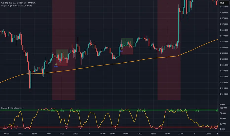
SuperTrend AI (Clustering) [LuxAlgo]The SuperTrend AI indicator is a novel take on bridging the gap between the K-means clustering machine learning method & technical indicators. In this case, we apply K-Means clustering to the famous SuperTrend indicator.
🔶 USAGE
Users can interpret the SuperTrend AI trailing stop similarly to the regular SuperTrend indicator. Using higher minimum/maximum factors will return longer-term signals.
The displayed performance metrics displayed on each signal allow for a deeper interpretation of the indicator. Whereas higher values could indicate a higher potential for the market to be heading in the direction of the trend when compared to signals with lower values such as 1 or 0 potentially indicating retracements.
In the image above, we can notice more clear examples of the performance metrics on signals indicating trends, however, these performance metrics cannot perform or predict every signal reliably.
We can see in the image above that the trailing stop and its adaptive moving average can also act as support & resistance. Using higher values of the performance memory setting allows users to obtain a longer-term adaptive moving average of the returned trailing stop.
🔶 DETAILS
🔹 K-Means Clustering
When observing data points within a specific space, we can sometimes observe that some are closer to each other, forming groups, or "Clusters". At first sight, identifying those clusters and finding their associated data points can seem easy but doing so mathematically can be more challenging. This is where cluster analysis comes into play, where we seek to group data points into various clusters such that data points within one cluster are closer to each other. This is a common branch of AI/machine learning.
Various methods exist to find clusters within data, with the one used in this script being K-Means Clustering , a simple iterative unsupervised clustering method that finds a user-set amount of clusters.
A naive form of the K-Means algorithm would perform the following steps in order to find K clusters:
(1) Determine the amount (K) of clusters to detect.
(2) Initiate our K centroids (cluster centers) with random values.
(3) Loop over the data points, and determine which is the closest centroid from each data point, then associate that data point with the centroid.
(4) Update centroids by taking the average of the data points associated with a specific centroid.
Repeat steps 3 to 4 until convergence, that is until the centroids no longer change.
To explain how K-Means works graphically let's take the example of a one-dimensional dataset (which is the dimension used in our script) with two apparent clusters:
This is of course a simple scenario, as K will generally be higher, as well the amount of data points. Do note that this method can be very sensitive to the initialization of the centroids, this is why it is generally run multiple times, keeping the run returning the best centroids.
🔹 Adaptive SuperTrend Factor Using K-Means
The proposed indicator rationale is based on the following hypothesis:
Given multiple instances of an indicator using different settings, the optimal setting choice at time t is given by the best-performing instance with setting s(t) .
Performing the calculation of the indicator using the best setting at time t would return an indicator whose characteristics adapt based on its performance. However, what if the setting of the best-performing instance and second best-performing instance of the indicator have a high degree of disparity without a high difference in performance?
Even though this specific case is rare its however not uncommon to see that performance can be similar for a group of specific settings (this could be observed in a parameter optimization heatmap), then filtering out desirable settings to only use the best-performing one can seem too strict. We can as such reformulate our first hypothesis:
Given multiple instances of an indicator using different settings, an optimal setting choice at time t is given by the average of the best-performing instances with settings s(t) .
Finding this group of best-performing instances could be done using the previously described K-Means clustering method, assuming three groups of interest (K = 3) defined as worst performing, average performing, and best performing.
We first obtain an analog of performance P(t, factor) described as:
P(t, factor) = P(t-1, factor) + α * (∆C(t) × S(t-1, factor) - P(t-1, factor))
where 1 > α > 0, which is the performance memory determining the degree to which older inputs affect the current output. C(t) is the closing price, and S(t, factor) is the SuperTrend signal generating function with multiplicative factor factor .
We run this performance function for multiple factor settings and perform K-Means clustering on the multiple obtained performances to obtain the best-performing cluster. We initiate our centroids using quartiles of the obtained performances for faster centroids convergence.
The average of the factors associated with the best-performing cluster is then used to obtain the final factor setting, which is used to compute the final SuperTrend output.
Do note that we give the liberty for the user to get the final factor from the best, average, or worst cluster for experimental purposes.
🔶 SETTINGS
ATR Length: ATR period used for the calculation of the SuperTrends.
Factor Range: Determine the minimum and maximum factor values for the calculation of the SuperTrends.
Step: Increments of the factor range.
Performance Memory: Determine the degree to which older inputs affect the current output, with higher values returning longer-term performance measurements.
From Cluster: Determine which cluster is used to obtain the final factor.
🔹 Optimization
This group of settings affects the runtime performances of the script.
Maximum Iteration Steps: Maximum number of iterations allowed for finding centroids. Excessively low values can return a better script load time but poor clustering.
Historical Bars Calculation: Calculation window of the script (in bars).

ai quant oculusAI QUANT OCULUS
Version 1.0 | Pine Script v6
Purpose & Innovation
AI QUANT OCULUS integrates four distinct technical concepts—exponential trend filtering, adaptive smoothing, momentum oscillation, and Gaussian smoothing—into a single, cohesive system that delivers clear, objective buy and sell signals along with automatically plotted stop-loss and three profit-target levels. This mash-up goes beyond a simple EMA crossover or standalone TRIX oscillator by requiring confluence across trend, adaptive moving averages, momentum direction, and smoothed price action, reducing false triggers and focusing on high‐probability turning points.
How It Works & Why Its Components Matter
Trend Filter: EMA vs. Adaptive MA
EMA (20) measures the prevailing trend with fixed sensitivity.
Adaptive MA (also EMA-based, length 10) approximates a faster-responding moving average, standing in for a KAMA-style filter.
Bullish bias requires AMA > EMA; bearish bias requires AMA < EMA. This ensures signals align with both the underlying trend and a more nimble view of recent price action.
Momentum Confirmation: TRIX
Calculates a triple-smoothed EMA of price over TRIX Length (15), then converts it to a percentage rate-of-change oscillator.
Positive TRIX reinforces bullish entries; negative TRIX reinforces bearish entries. Using TRIX helps filter whipsaws by focusing on sustained momentum shifts.
Gaussian Price Smoother
Applies two back-to-back 5-period EMAs to the price (“gaussian” smoothing) to remove short-term noise.
Price above the smoothed line confirms strength for longs; below confirms weakness for shorts. This layer avoids entries on erratic spikes.
Confluence Signals
Buy Signal (isBull) fires only when:
AMA > EMA (trend alignment)
TRIX > 0 (momentum support)
Close > Gaussian (price strength)
Sell Signal (isBear) fires under the inverse conditions.
Requiring all three conditions simultaneously sharply reduces false triggers common to single-indicator systems.
Automatic Risk & Reward Plotting
On each new buy or sell signal (edge detection via not isBull or not isBear ), the script:
Stores entryPrice at the signal bar’s close.
Draws a stop-loss line at entry minus ATR(14) × Stop Multiplier (1.5) by default.
Plots three profit-target lines at entry plus ATR × Target Multiplier (1×, 1.5×, and 2×).
All previous labels and lines are deleted on each new signal, keeping the chart uncluttered and focusing only on the current trade.
Inputs & Customization
Input Description Default
EMA Length Period for the main trend EMA 20
Adaptive MA Length Period for the faster adaptive EM A substitute 10
TRIX Length Period for the triple-smoothed momentum oscillator 15
Dominant Cycle Length (Reserved) 40
Stop Multiplier ATR multiple for stop-loss distance 1.5
Target Multiplier ATR multiple for first profit target 1.5
Show Buy/Sell Signals Toggle on-chart labels for entry signals On
How to Use
Apply to Chart: Best on 15 m–1 h timeframes for swing entries or 5 m for agile scalps.
Wait for Full Confluence:
Look for the AMA to cross above/below the EMA and verify TRIX and Gaussian conditions on the same bar.
A bright “LONG” or “SHORT” label marks your entry.
Manage the Trade:
Place your stop where the red or green SL line appears.
Scale or exit at the three yellow TP1/TP2/TP3 lines, automatically drawn by volatility.
Repeat Cleanly: Each new signal clears prior annotations, ensuring you only track the active setup.
Why This Script Stands Out
Multi-Layer Confluence: Trend, momentum, and noise-reduction must all align, addressing the weaknesses of single-indicator strategies.
Automated Trade Management: No manual plotting—stop and target lines appear seamlessly with each signal.
Transparent & Customizable: All logic is open, adjustable, and clearly documented, allowing traders to tweak lengths and multipliers to suit different instruments.
Disclaimer
No indicator guarantees profit. Always backtest AI QUANT OCULUS extensively, combine its signals with your own analysis and risk controls, and practice sound money management before trading live.

AI QUANT OCULUSAI QUANT OCULUS
Version 1.0 | Pine Script v6
Purpose & Innovation
AI QUANT OCULUS integrates four distinct technical concepts—exponential trend filtering, adaptive smoothing, momentum oscillation, and Gaussian smoothing—into a single, cohesive system that delivers clear, objective buy and sell signals along with automatically plotted stop-loss and three profit-target levels. This mash-up goes beyond a simple EMA crossover or standalone TRIX oscillator by requiring confluence across trend, adaptive moving averages, momentum direction, and smoothed price action, reducing false triggers and focusing on high‐probability turning points.
How It Works & Why Its Components Matter
Trend Filter: EMA vs. Adaptive MA
EMA (20) measures the prevailing trend with fixed sensitivity.
Adaptive MA (also EMA-based, length 10) approximates a faster-responding moving average, standing in for a KAMA-style filter.
Bullish bias requires AMA > EMA; bearish bias requires AMA < EMA. This ensures signals align with both the underlying trend and a more nimble view of recent price action.
Momentum Confirmation: TRIX
Calculates a triple-smoothed EMA of price over TRIX Length (15), then converts it to a percentage rate-of-change oscillator.
Positive TRIX reinforces bullish entries; negative TRIX reinforces bearish entries. Using TRIX helps filter whipsaws by focusing on sustained momentum shifts.
Gaussian Price Smoother
Applies two back-to-back 5-period EMAs to the price (“gaussian” smoothing) to remove short-term noise.
Price above the smoothed line confirms strength for longs; below confirms weakness for shorts. This layer avoids entries on erratic spikes.
Confluence Signals
Buy Signal (isBull) fires only when:
AMA > EMA (trend alignment)
TRIX > 0 (momentum support)
Close > Gaussian (price strength)
Sell Signal (isBear) fires under the inverse conditions.
Requiring all three conditions simultaneously sharply reduces false triggers common to single-indicator systems.
Automatic Risk & Reward Plotting
On each new buy or sell signal (edge detection via not isBull or not isBear ), the script:
Stores entryPrice at the signal bar’s close.
Draws a stop-loss line at entry minus ATR(14) × Stop Multiplier (1.5) by default.
Plots three profit-target lines at entry plus ATR × Target Multiplier (1×, 1.5×, and 2×).
All previous labels and lines are deleted on each new signal, keeping the chart uncluttered and focusing only on the current trade.
Inputs & Customization
Input Description Default
EMA Length Period for the main trend EMA 20
Adaptive MA Length Period for the faster adaptive EM A substitute 10
TRIX Length Period for the triple-smoothed momentum oscillator 15
Dominant Cycle Length (Reserved) 40
Stop Multiplier ATR multiple for stop-loss distance 1.5
Target Multiplier ATR multiple for first profit target 1.5
Show Buy/Sell Signals Toggle on-chart labels for entry signals On
How to Use
Apply to Chart: Best on 15 m–1 h timeframes for swing entries or 5 m for agile scalps.
Wait for Full Confluence:
Look for the AMA to cross above/below the EMA and verify TRIX and Gaussian conditions on the same bar.
A bright “LONG” or “SHORT” label marks your entry.
Manage the Trade:
Place your stop where the red or green SL line appears.
Scale or exit at the three yellow TP1/TP2/TP3 lines, automatically drawn by volatility.
Repeat Cleanly: Each new signal clears prior annotations, ensuring you only track the active setup.
Why This Script Stands Out
Multi-Layer Confluence: Trend, momentum, and noise-reduction must all align, addressing the weaknesses of single-indicator strategies.
Automated Trade Management: No manual plotting—stop and target lines appear seamlessly with each signal.
Transparent & Customizable: All logic is open, adjustable, and clearly documented, allowing traders to tweak lengths and multipliers to suit different instruments.
Disclaimer
No indicator guarantees profit. Always backtest AI QUANT OCULUS extensively, combine its signals with your own analysis and risk controls, and practice sound money management before trading live.

AI Money FlowAI Money Flow is a revolutionary trading indicator that combines cutting-edge artificial intelligence technologies with traditional Smart Money concepts. This indicator provides comprehensive market analysis with emphasis on signal accuracy and reliability.
Key Features:
Volume Profile with Smart Money Analysis - Displays real money flow instead of just volume, identifying key support and resistance levels based on actual trader activity.
Volatility-Based Support & Resistance - Intelligent support and resistance levels that dynamically adapt to market volatility in real-time for maximum accuracy.
Order Flow Analysis - Advanced detection of buying and selling pressure that reveals the true intentions of large market players.
Machine Learning Optimization - Futuristic AI technology that automatically learns and optimizes settings for each specific asset and timeframe.
Risk Management - Advanced volatility and price spike detection for better risk management and capital protection.
Real-time Dashboard - Modern dashboard with color-coded signals provides instant overview of market conditions and trends.
Accuracy: 88-93%

AI Volume SignalsAI Volume Signals
The AI Volume Signals indicator detects significant volume spikes and combines them with trend direction and candle color to generate buy and sell signals. This script utilizes an Exponential Moving Average (EMA) of volume to detect abnormal volume spikes, which could indicate strong market activity. It also filters signals based on the trend direction determined by a 50-period EMA of the price.
Key Features:
Volume Spike Detection: The indicator detects when the current volume exceeds the EMA of volume by a user-defined multiplier, signaling an unusual increase in market activity.
Trend Direction Filter: The 50-period EMA of the price is used to determine the market trend. Buy signals are generated when the price is above the EMA (uptrend), and sell signals occur when the price is below the EMA (downtrend).
Candle Color Filter: The indicator only generates a buy signal when the current candle is bullish (green), and a sell signal when the current candle is bearish (red).
Optional Volume EMA Line: A customizable option allows users to toggle the visibility of the Volume EMA line on the chart. By default, the line is hidden, but can be enabled in the settings.
Signals:
Buy Signal: Generated when a volume spike occurs, the trend is upward, and the current candle is bullish.
Sell Signal: Generated when a volume spike occurs, the trend is downward, and the current candle is bearish.
Alerts:
Buy Alert: Alerts the user when a buy signal is triggered.
Sell Alert: Alerts the user when a sell signal is triggered.
Visualization:
Buy Signal: A green label appears below the bar when the buy conditions are met.
Sell Signal: A red label appears above the bar when the sell conditions are met.
Volume EMA: A line representing the EMA of the volume is plotted on the chart for reference. The visibility of this line can be toggled in the settings.
This indicator can help traders identify potential entry points based on increased volume activity while considering trend direction and candlestick patterns.
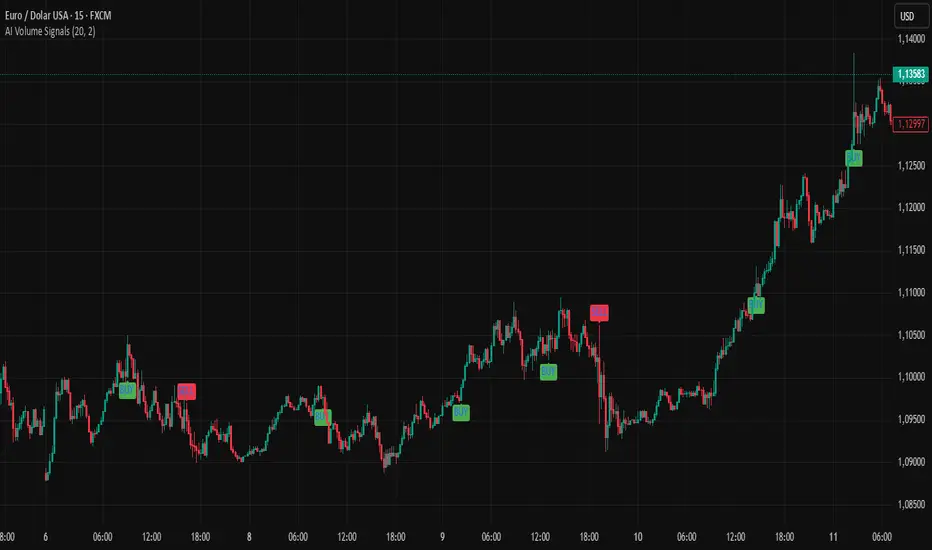
Crypto Index Creator (MEMES & AI Supercycle Dominance, etc)This indicator aims to help to create any INDEX desired including but not limited to its Market Cap and Dominance on the crypto market.
This script was inspired originally by Murad's "Memecoins Dominance" but then I extended it to AI and can be extended to anything in fact, so you can create any index!
I made each token entry editable so that the script can survive the evolution of time as likely projects and INDEXES are going to change a lot, so that you can add/modify your own indices of preference if not listed by default and in order to make it future proof.
You can play with the settings, can compare to BTC, ETC, SOL, etc. for helping in your studies
You also have the option to check the info of each symbol on a table available on the settings, in order to help you figure out if there are any errors and also help you to easily check how the symbols are performing individually
Notes:
- Many projects are not like MEMECOINS that have fixed supply, normally VC projects have a very variable circulating supply, so you might want to update the info of the circulating supply for your projects to make it more accurate if you desire.
- For this script there is a limit of 32 Symbols, due to tradingview own limits, yet you can always "add" multiple projects per line as long as their circulating supply is the same.
- You might want to edit/sort the tickers of the top3, top5 and top10 if they follow bellow those top ranks, but this is not necessary if you don't care about Top 3-10 specific calculations.
- My default "indices" were made of token selections of mine as of November 2024, those defaults indices/tickers I might or might not update them eventually but you are free to adapt/modify the tickers in the settings as history evolves, and you can leave your own indexes on the comment section of this post for others to use
- As you might not be able to create/store multiple different indexes at the same time, you might want to add this indicator multiple times on your screen and then modify the tickers of each instance of this indicator, by that you can have multiple indexes.

AI Exclusive(Precision Entry)AI Exclusive (Precision Entry)
Overview: An indicator that provides precise entry signals along with defined Take Profit (TP) and Stop Loss (SL).
Benefits:
• Confident entries with built in risk management
• Clear TP and SL displayed on the chart
• Suitable for both beginner and professional traders
Features:
• Transparent, unambiguous signals
• Usable on all symbols and timeframes
• Visual design with colored lines and clear labels
