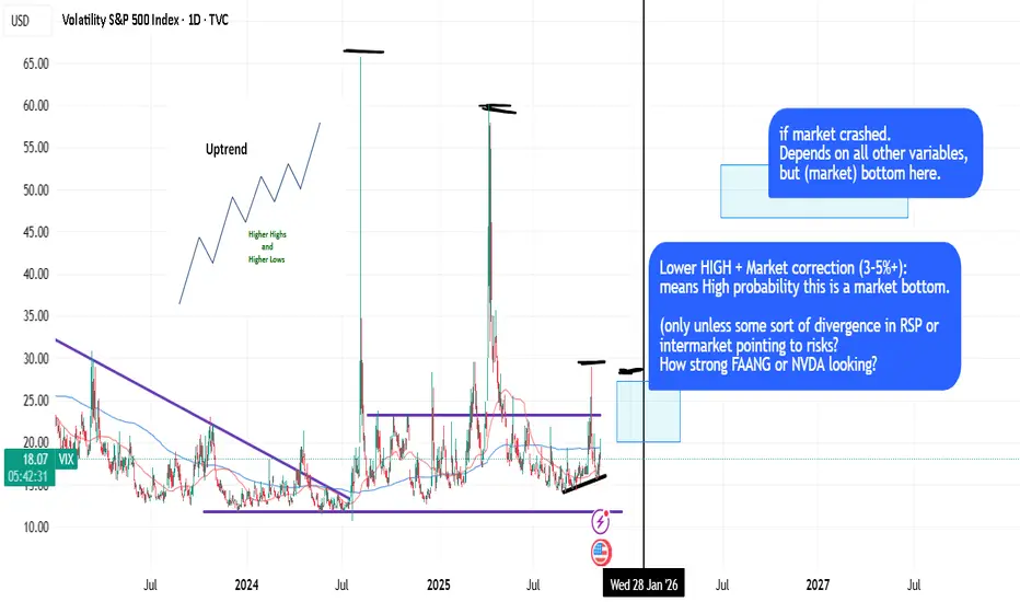
VIX: Fear vs Correction principleBased on principle, where highest probability is when:
-(SPX) 50/200 UP sloping.
-Full correction
-Positive "context" (fundamentals, that change every year. For instance next year theme is new FED chair. Beginning of QE money printing etc).
Some times SPX drops and VIX flies on "fear". but strong trend stays in tact. And sometimes there is a full exhaust, meaning going up is "easy" (no resistance).
Probability

BTC 80% Chance of Another Low, BUT First...On 11/22/25 , Bitcoin experienced a relatively rare event: the Daily RSI dropped below 26 . On the Coinbase COINBASE:BTCUSD chart, this has occurred only 20 times historically since December 2014. By analyzing the price action following each occurrence, we can estimate the probability of future behavior when RSI reaches these extreme levels.
The results of each occurrence are summarized in the table shown on the chart.
The table includes:
Dates when RSI fell below 26
Whether price eventually made a lower low ( 16 out of 20 times, or 80% )
Maximum bullish move from the Daily swing low close to the highest wick before correcting (average +16% )
Time to reach that swing high (average 8 days )
Time to reach a new lower low (average 22 days )
The 16 times price eventually made lower low are marked with red or purple vertical lines . The 4 times it did not make a lower low are marked with green vertical lines .
Key Observations
When RSI drops below 26, it typically signals strong bearish momentum , but it is also often followed by a bullish RSI divergence as price forms a higher low in momentum. Historically, a lower low formed 80% of the time , suggesting a high probability of another downside move for BTC in the weeks ahead.
At present:
RSI bottomed at 22.93 on 11/22/25
BTC has already rallied ~11% from the swing low
We are currently at day 21 without a new lower low
All of these metrics remain well within historical norms .
However, there is an interesting nuance. Of the 16 cases where a lower low eventually formed , only 4 took more than 20 days to do so . In all 4 cases (marked with purple vertical lines) , BTC tested the Weekly 12 EMA before making the next leg lower (with a minor exception on the11/24/19 case, where a marginal lower low formed before a strong push above the Weekly 12 EMA).
The Weekly 12 EMA currently sits around $100,000 , suggesting BTC may test this level before any further meaningful correction.
ACTIONALBLE SCENARIOS
If this is a bear market:
Passive investors: Continue dollar-cost averaging at your preferred interval.
Active investors: Consider taking partial or full profits if BTC trades above $100,000 . Set calendar alerts for October 2026 and/or below $50,000 to resume heavier accumulation when BTC may bottom this bear cycle.
Swing traders: Consider Long setups below $86,800 with a stop-loss at $83,500, targeting the Weekly 12 EMA (~$100,000) , with an extended target around $101,000 .
If this is still a bull market:
Price will likely make a lower low to below $80,000 before a bullish move.
Passive investors: Continue dollar-cost averaging.
Active investors / swing traders: Continue accumulating below $86,800 , with heavier accumulation around $78,370 .
Hope this study helps add context to current price action. Trade safe everyone, PEACE.

The Bell Curve: Understanding Normal Distribution in TradingMost traders have seen the “bell curve” at some point, but very few actually use it when they think about risk and returns.
If you really understand the normal distribution, you’re already thinking more like a risk manager than a gambler.
1. What is the normal distribution?
The normal distribution is a probability distribution that describes how values tend to cluster around an average.
If you plotted a huge number of outcomes (for example, daily returns or P&L per trade), the shape you’d get would often look like a symmetric bell :
- Most observations are close to the center.
- As you move away from the center in either direction, outcomes become less frequent.
- Extreme gains and losses are possible, but they’re relatively rare.
Mathematically, a normal distribution is usually written as N(μ, σ):
μ (mu) is the mean – the average outcome.
σ (sigma) is the standard deviation – a measure of how widely the outcomes are spread around that mean.
In trading terms:
If your returns roughly follow a normal distribution, you should expect many small wins and losses clustered near zero, and only occasional large moves in either direction.
2. Mean (μ): the “drift” of your system
The mean is the point at the center of the distribution. On a chart of returns, this is where the bell is highest.
If μ > 0, the bell is shifted slightly to the right → your system is profitable on average.
If μ < 0, it’s shifted to the left → your system slowly loses money over time.
For a trading strategy, μ is basically your edge. It doesn’t need to be huge. Even a small positive mean return, if it’s consistent and combined with disciplined risk management, can compound strongly over the long run.
3. Standard deviation (σ): volatility in one number
The standard deviation controls how wide or narrow the bell curve is.
- A small σ gives a tall, narrow bell → outcomes are tightly clustered around the mean.
- A large σ gives a short, wide bell → outcomes are more spread out, with bigger swings away from the mean.
Think of σ as a statistical way to describe volatility:
- For an asset: how much its price typically moves relative to its average change.
- For your strategy: how much your returns or daily P&L fluctuate.
Two systems can have the same mean return but very different σ:
- System A: μ = 0.2%, σ = 0.5% → relatively smooth ride.
- System B: μ = 0.2%, σ = 2% → same edge, but a wild equity curve and deeper drawdowns.
Same average, totally different emotional and risk profile.
4. The 68–95–99.7 rule
One of the most useful features of the normal distribution is how predictable it is. Roughly:
- About 68.2% of observations lie within ±1σ of the mean.
- About 95.4% lie within ±2σ.
- About 99.7% lie within ±3σ.
So if daily returns of an asset were approximately normal with:
- Mean μ = 0.1%
- Standard deviation σ = 1%
Then under that model you’d expect:
- Roughly 68% of days between –0.9% and +1.1%
- Roughly 95% of days between –1.9% and +2.1%
- Only about 0.3% of days beyond ±3%
Anything far outside that ±3σ range is, in theory, a very rare event. In practice, that’s often the kind of day everyone remembers.
5. Why this matters for traders
Even with all its limitations, the normal distribution is a powerful framework for thinking about risk:
Position sizing
If you know (or estimate) the standard deviation of your returns, you can form an idea of what “normal” daily or weekly swings look like, and size positions so those swings are survivable.
Stop-loss logic
Stops that sit right in the middle of the usual noise (within about ±1σ) will get hit constantly.
Stops closer to the ±2σ–3σ region are more aligned with “something unusual is happening, I want to be out.”
Expectation management
Most days and most trades will fall inside the “boring” part of the bell curve.
Understanding that prevents you from overtrading while you wait for the edges of the distribution – the bigger opportunities.
6. The catch: markets are not perfectly normal
Real markets often break the textbook assumptions:
- Returns tend to have fat tails → extreme moves happen more often than a normal distribution would predict.
- Distributions are often skewed → one side (usually the downside) has more frequent or more severe extreme events.
That means:
- A move that looks like a “5σ event” under a normal model might actually be something that happens every few years.
- Risk models based strictly on normal assumptions usually underestimate crash risk.
- Strategies like option selling can look very safe when you only think in terms of a normal distribution, but they are very sensitive to those fat tails.
So the normal distribution should be treated as a baseline model, not as reality itself.
7. Quick recap
The normal distribution is the classic bell curve that describes how values cluster around an average.
It’s parameterized by μ (mean) and σ (standard deviation).
Roughly 68% / 95% / 99.7% of observations lie within 1σ / 2σ / 3σ of the mean in a perfectly normal world.
Markets only approximate this; they usually show fat tails and skew, so extreme events are more common than the simple model suggests.
Even with those limitations, it’s a very useful tool for thinking about returns, drawdowns, and the range of outcomes you should be prepared for.
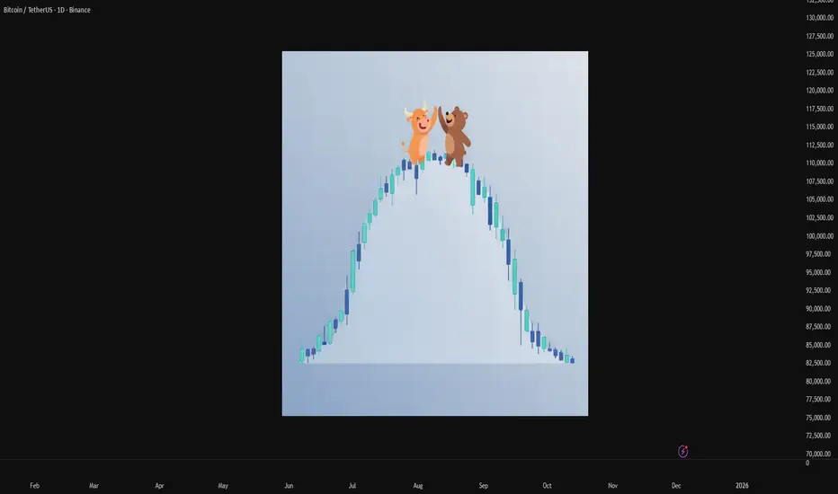
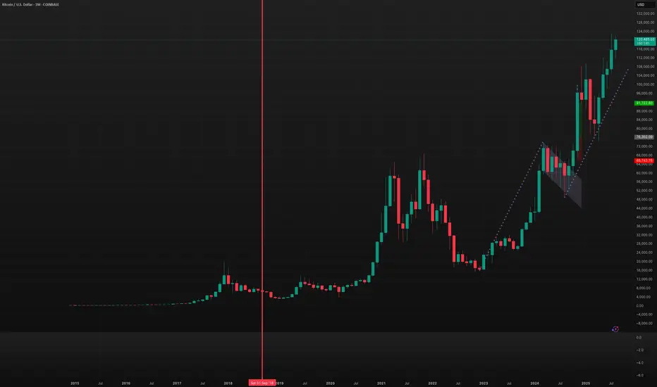
Markets are predictable. Trading S/D imbalances.Pre-election. 1200% extension after a 2-year rally. Facing ATH with strong trend and expectations.
This is a rule or factorial based approach. What most people think - is usually how most people are positioned, or usually also is the logical truth.
When something extends... and some risks emerge -- you can't really trust charts (ie demand strength). that's a prejudgement? ie sloppy way to look at things.
Also somewhat predictable is the 2 year rally, 3rd year weakness. If markets stall -- markets sells off on expectations of that "rule" lol
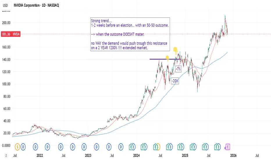
NVDA: 1 week before earnings effect. Supply-demand imbalance.Parretto principle (20-80): small important things can have great influence in grand scheme of things. Some events have greater weight, than say 80-90% of daily events.
Stocks move based on Supply-demand dynamics (disbalance etc), patterns or trends are just a feedback.
The problem with using charts as a feedback for strength (or feedback for S-D strength) is that: (1) on a expensive market, with extended prices (with high supply too), (2) during important NVDA earnings, it's almost predictable how markets would sink, or at least be volatile.
Demand stalls. Supply gets worried. Price down.
//People are risk averse. Hence.. predictable.

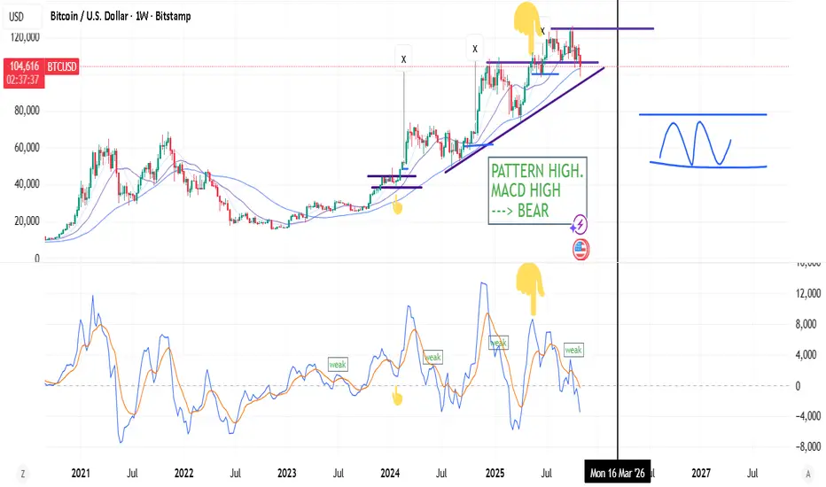
PATTERN logic + MACD LOWS/POTENCIAL = High probabilities.If you combine basic FACTORS of Patterns + MACD (weaknesses or Lows/Highs) you get pretty straightforward probability.
Weekly MACD above zero (and daily macd above zero) mean strong impulse, trend. But sometimes deep corrections in negative territory (bears) are not negative, because every chart pattern require strong "push" to break the pattern. I think you can see if there's smoke, in advance.
Using HLOW/LHIGH (Dow) + LOGIC to pinpoint probabilities.DOW Theory is the king of the stock market (Higher Lows, Lower Highs, uptrending, etc.) and it's quite basic concept to apply with logic.
Sometimes you can time the market (based on 50dma/200dma crosses, price extensions) and LHIGH dynamics and logic -> to pinpoint probabilities. Like, look at VIX dynamics during 2023/2024.
in short: DOW + LOGIC = PROBABILITY.
Bitcoin Loves OctoberRecently I had a client ask if I could tell them the probability of a candle being bullish or bearish. My fingers got excited and I tried it out. Little did I know this rabbit hole was getting adventurous.
July this month, COINBASE:BTCUSD rose by 8%. The probability read 70% which now makes it 78% next year. Whats even more curious is that October has a 90% chance of having a buillish candle.
Now the question remains, will this october be the one to lower this score or raise it?
Lets wait and find out.
Trading is the Game of ProbabilitiesMost traders start with one simple goal ➜ to be right all the time
🔲Right about the trend.
🔲Right about the breakout.
🔲Right about the trade.
But here’s the truth - 'the market doesn’t care who’s right'.
↳ Even the best analysis fails sometimes.
↳ Even the weakest setup works sometimes.
Because trading isn’t a test of accuracy, it’s a test of managing what is more probable.
↳ Profitable traders don’t chase perfection.
↳ They focus on risk, reward, and consistency.
We can be wrong 6 times out of 10...
And still make money if our winners are bigger than our losers.
↳ Trading success is not about predicting.
↳ It’s about positioning and managing our trade.
We manage risk when the odds are low.
We maximize reward when the odds are high.
The shift happens when we stop trying to be right...
and start thinking in probabilities.
That’s when we stop gambling and start profitable trading.
Are you playing casino or managing your risk?
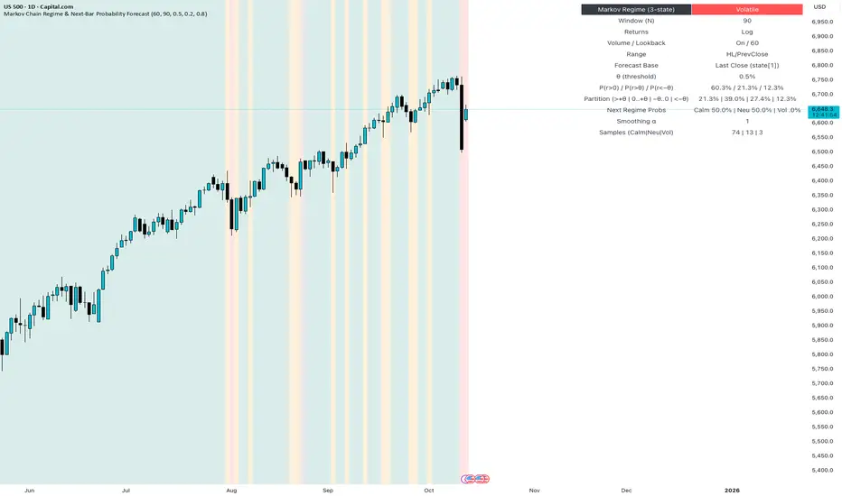
HOW-TO: Forecast Next-Bar Odds with Markov ProbCast🎯 Goal
In 5 minutes, you’ll add Markov ProbCast to a chart, calibrate the “big-move” threshold θ for your instrument/timeframe, and learn how to read the next-bar probabilities and regime signals
(🟩 Calm | 🟧 Neutral | 🟥 Volatile).
🧩 Add & basic setup
Open any chart and timeframe you trade.
Add Markov ProbCast — P(next-bar) Forecast Panel from the Public Library (search “Markov ProbCast”).
Inputs (recommended starting point):
• Returns: Log
• Include Volume (z-score): On (Lookback = 60)
• Include Range (HL/PrevClose): On
• Rolling window N (transitions): 90
• θ as percent: start at 0.5% (we’ll calibrate next)
• Freeze forecast at last close: On (stable readings)
• Display: leave plots/partition/samples On
📏 Calibrate θ (2-minute method)
Pick θ so the “>+θ” bucket truly flags meaningful bars for your market & timeframe. Try:
• If intraday majors / large caps: θ ≈ 0.2%–0.6% on 1–5m; 0.3%–0.8% on 15–60m.
• If high-vol crypto / small caps: θ ≈ 0.5%–1.5% on 1–5m; 0.8%–2.0% on 15–60m.
Then watch the Partition row for a day: if the “>+θ” bucket is almost never triggered, lower θ a bit; if it’s firing constantly, raise θ. Aim so “>+θ” captures move sizes you actually care about.
📖 Read the panel (what the numbers mean)
• P(next r > 0) : Directional tilt for the very next candle.
• P(next r > +θ) : Odds of a “big” upside move beyond your θ.
• P(next r < −θ) : Odds of a “big” downside move.
• Partition (>+θ | 0..+θ | −θ..0 | <−θ): Four buckets that ≈ sum to 100%.
• Next Regime Probs : Chance the market flips to 🟩 Calm / 🟧 Neutral / 🟥 Volatile next bar.
• Samples : How many historical next-bar examples fed each next-state estimate (confidence cue).
Note: Heavy calculations update on confirmed bars; with “Freeze” on, values won’t flicker intrabar.
📚 Two practical playbooks
Breakout prep
• Watch P(next r > +θ) trending up and staying elevated (e.g., > 25–35%).
• A rising Next Regime: Volatile probability supports expansion context.
• Combine with your trigger (structure break, session open, liquidity sweep).
Mean-reversion defense
• If already long and P(next r < −θ) lifts while Volatile odds rise, consider trimming size, widening stops, or waiting for a better setup.
• Mirror the logic for shorts when P(next r > +θ) lifts.
⚙️ Tuning & tips
• N=90 balances adaptivity and stability. For very fast regimes, try 60; for slower instruments, 120.
• Keep Freeze at close on for cleaner alerts/decisions.
• If Samples are small and values look jumpy, give it time (more bars) or increase N slightly.
🧠 Why this works (the math, briefly)
We learn a 3-state regime and its transition matrix A (A = P(Sₜ₊₁=j | Sₜ=i)), estimate next-bar event odds conditioned on the next state (e.g., q_gt(j)=P(rₜ₊₁>+θ | Sₜ₊₁=j)), then forecast by mixing:
P(event) = Σⱼ A · q(event | next=j).
Laplace/Beta smoothing, per-state sample gating, and unconditional fallbacks keep estimates robust.
❓FAQ
• Why do probabilities change across instruments/timeframes? Different volatility structure → different transitions and conditional odds.
• Why do I sometimes see “…” or NA? Not enough recent samples for a next-state; the tool falls back until data accumulate.
• Can I use it standalone? It’s a context/forecast panel—pair it with your entry/exit rules and risk management.
📣 Want more?
If you’d like an edition with alerts , σ-based θ, quantile regime cutoffs, and a compact ribbon—or a full strategy that uses these probabilities for entries, filters, and sizing—please Like this post and comment “Pro” or “Strategy”. Your feedback decides what we release next.
BTC WILL NOT BE THERE🪙 CRYPTOCAP:BTC October 10th 😅 Straddle breakevens:
118000 & 127000
🪙 CRYPTOCAP:BTC October 17th 😅 Straddle breakevens:
116000 & 130000
σ Sigma probabilities:
October 10th
| σ | Multiplier × 😅 | Probability
| 1σ | 117000 & 128000 | ≈68%
| 2σ | 112000 & 133000 | ≈95%
October 17th
| σ | Multiplier × 😅 | Probability
| 1σ | 114000 & 131000 | ≈68%
| 2σ | 106000 & 139000 | ≈95%

The Options Mirage: The Jackpot That’s Rigged Against YouMost retail traders fall in love with options because they seem to offer the impossible: with just a few hundred dollars you can dream of outsized returns. Fast money, easy money—at least that’s the story. With the right broker account and a handful of trades, the dream of becoming rich feels just around the corner.
What you’re not told—and what few truly understand given the complexity of the product—is that the “explosive payout” is not an opportunity. It’s a price. A very high one. And often inflated by the industry itself, knowing that the average investor (or rather, gambler) has no real way to calculate what they’re actually paying for. What you’re really buying is access to an extremely low probability of success, dressed up as a sophisticated strategy.
Yes, it’s the same psychology that drives lotteries and sports betting. And in finance, the odds aren’t any kinder.
The Baseline: the Where
At its simplest, speculation is about anticipating an up or down move in price.
Think it’s going up? Buy and aim to sell higher.
Think it’s going down? Sell and aim to buy back lower.
It sounds simple, but anyone with more than a month of trading experience can tell you it’s anything but. No one can predict the future with certainty. Still, this is at least a binary game: two mutually exclusive outcomes, like flipping a coin.
In technical terms, the market starts as a 50/50 distribution. With skill, analysis, and discipline, you might bias those odds slightly—say, 60/40 in your favor. That bias, repeated consistently, is what we call an edge. And with an edge, the path to long-term success is paved.
The Illusion of Acceleration
But let’s be honest: who wants to grind out a 60/40 edge slowly? We’re here for the Lamborghini, right? And the sooner the better.
That’s where the industry steps in with its “solution”: options. The promise is seductive—leverage the process, accelerate the outcome. With little money down, you can aim for massive returns. What’s not to like?
The problem is that the acceleration doesn’t come for free. To deliver those explosive payouts, the game adds layers of complexity.
From Where… to How and When
In options, you don’t just need to be right about where price is going.
You also need to be right about how it moves. That’s volatility—the speed and amplitude of the move. Even if you guess the direction correctly, if the move isn’t strong enough to beat strike + premium, you lose.
And then comes the when. Options expire. Time works against you. With the rise of 0DTE options, this window has shrunk to a single day. You might be perfectly right on direction and volatility—but if it happens tomorrow instead of today, your trade is worthless.
Now here’s the key point: this isn’t additive complexity. It’s multiplicative. Each layer collapses your probability of success exponentially. Even though the mathematical proof could be enlightening, I have promised not to use heavy math in this blog. All you need to know is this: in the majority of cases, that collapse in probability is not evenly compensated by the outsized payout. And this is exactly what most retail traders fail to perceive.
It’s not just that you’re playing a harder game—it’s that you’re playing a biased one, where the odds are stacked even further against you.
The Lottery Bias: The Cognitive Trap
Here’s where psychology plays its cruelest trick. The lower the probability of success, the higher the payout offered. In fact, it’s not even the full payout you deserve—it’s a discounted, haircut payout, cleverly packaged so you don’t notice because the potential number is so large. And that number lights up the brain like a jackpot.
The industry knows this. It builds its business on the fact that humans systematically overestimate tiny probabilities and underestimate the certainty of losing. Retail traders convince themselves they’re being clever: risking little for the chance at something huge. But the math is merciless—the expected value is brutally negative.
The market is not handing you an edge. It’s dismantling any possibility you had of one. That giant payout you see? It’s not a gift—it’s a warning label.
And yes, I know you can point to stories about the guy who hit the jackpot, who “proved the math wrong.” But let me ask you this: do you know what survivorship bias is? If you don’t, and you’re trading options, here’s some professional advice for free—go and read about it before you place your next trade.
The Real Path to the Lambo
What gets sold as “smart leverage” is, in truth, just a lottery ticket wearing a suit. The Lambo doesn’t come from hitting jackpots. It comes from consistency—from repeating disciplined decisions with positive expectancy until compounding does its quiet but powerful work.
And yes, I know most traders are in a hurry. The good news? The process can be accelerated—but not by gambling on options with negative expectancy. It can be accelerated using technical, rational tools. Once an edge is established, leverage makes sense. That’s where concepts like the Kelly criterion come in: scaling growth aggressively, but without walking straight into ruin. (I’ve already written about Kelly earlier in this blog: here.)
Conclusion
We’ve stripped the illusion bare: more conditions don’t make you smarter, they make you less likely to succeed. What feels like a shortcut is nothing more than a statistical mirage—the financial equivalent of a lottery ticket, marketed to you as a “highway to riches,” exploiting your belief that complexity equals intelligence.
Unfortunately, the narrative is powerful, because it preys directly on cognitive bias. I know I’m swimming against the tide here. I know this post won’t go viral. I don’t expect many to believe what the math has to say about options trading.
But maybe, just maybe, a small number of traders reading this will see beneath the surface and save their time, energy, and money for better pursuits. If that’s you, then this post has already done its job.
If you can resist the mirage and stick to building real edges, you’ve already won a key battle—and most likely saved yourself a costly trading lesson.

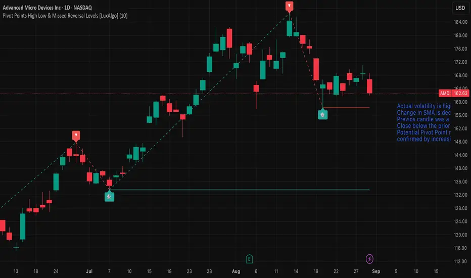
AMD — Watch for Pivot Reversal or Trend ContinuationMarket view
Actual volatility is high, confirmed by the Volatility Bars indicator.
The rate of change in the SMA is decreasing, suggesting momentum is weakening.
The previous candle was a Doji, indicating short-term indecision.
Price closed below the prior day’s low, adding bearish pressure.
A potential Pivot Point reversal is forming.
This reversal setup is confirmed by increasing Convolution Probability, supporting a higher chance of a directional move.
Trade plan
Long (trend continuation): buy on a break above the August 19, 2025 open.
Short (reversal): sell on a break below the pivot reversal at 158.25.
Stop-loss and position sizing: use volatility-based stops (e.g., ATR multiple) and risk no more than a small fixed percentage of capital per trade.
Trading as a Probabilistic ProcessTrading as a Probabilistic Process
As mentioned in the previous post , involvement in the market occurs for a wide range of reasons, which creates structural disorder. As a result, trading must be approached with the understanding that outcomes are variable. While a setup may reach a predefined target, it may also result in partial continuation, overextension, no follow-through, or immediate reversal. We trade based on known variables and informed expectations, but the outcome may still fall outside them.
Therefore each individual trade should be viewed as a random outcome. A valid setup could lose; an invalid one could win. It is possible to follow every rule and still take a loss. It is equally possible to break all rules and still see profits. These inconsistencies can cluster into streaks, several wins or losses in a row, without indicating anything about the applied system.
To navigate this, traders should think in terms of sample size. A single trade provides limited insight, relevant information only emerges over a sequence of outcomes. Probabilistic trading means acting on repeatable conditions that show positive expectancy over time, while accepting that the result of any individual trade is unknowable.
Expected Value
Expected value is a formula to measure the long-term performance of a trading system. It represents the average outcome per trade over time, factoring in both wins and losses:
Expected Value = (Win Rate × Average Win) – (Loss Rate × Average Loss)
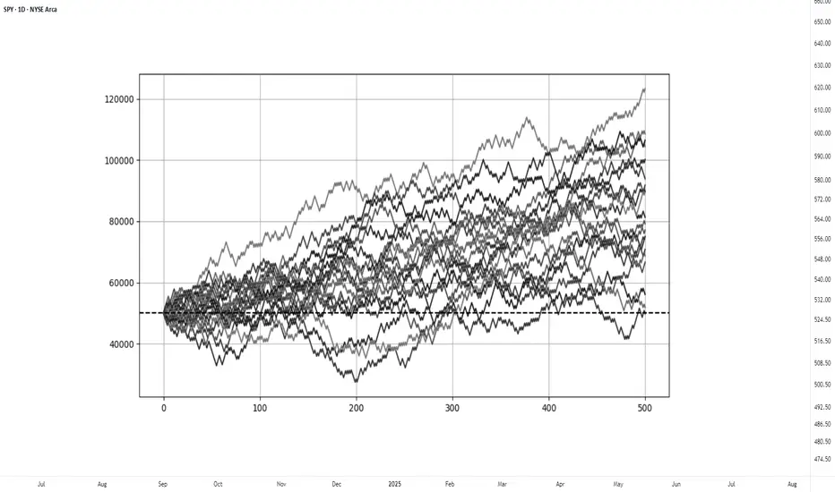
This principle can be demonstrated through simulation. A basic system with a 50% win rate and a 1.1 to 1 reward-to-risk ratio was tested over 500 trades across 20 independent runs. Each run began with a $50,000 account and applied a fixed risk of $1000 per trade. The setup, rules, and parameters remained identical throughout; the only difference was the random sequence in which wins and losses occurred.
While most runs clustered around a profitable outcome consistent with the positive expected value, several outliers demonstrated the impact of sequencing. When 250 trades had been done, one account was up more than 60% while another was down nearly 40%. In one run, the account more than doubled by the end of the 500 trades. In another, it failed to generate any meaningful profit across the entire sequence. These differences occurred not because of flaws in the system, but because of randomness in the order of outcomes.
These are known as Monte Carlo simulations, a method used to estimate possible outcomes of a system by repeatedly running it through randomized sequences. The technique is applied in many fields to model uncertainty and variation. In trading, it can be used to observe how a strategy performs across different sequences of wins and losses, helping to understand the range of outcomes that may result from probability.
Trading System Variations
Two different strategies can produce the same expected value, even if they operate on different terms. This is not a theoretical point, but a practical one that influences what kind of outcomes can be expected.
For example, System A operates with a high win rate and a lower reward-to-risk ratio. It wins 70% of the time with a 0.5 R, while System B takes the opposite approach and wins 30% of the time with a 2.5 R. If the applied risk is $1,000, the following results appear:
System A = (0.70 × 500) − (0.30 × 1,000) = 350 − 300 = $50
System B = (0.30 × 2,500) − (0.70 × 1,000) = 750 − 700 = $50
Both systems average a profit of $50 per trade, yet they are very different to trade and experience. Both are valid approaches if applied consistently. What matters is not the math alone, but whether the method can be executed consistently across the full range of outcomes.
Let’s look a bit closer into the simulations and practical implications.
The simulation above shows the higher winrate, lower reward system with an initial $100,000 balance, which made 50 independent runs of 1000 trades each. It produced an average final balance of $134,225. In terms of variance, the lowest final balance reached $99,500 while the best performer $164,000. Drawdowns remained modest, with an average of 7.67%, and only 5% of the runs ended below the initial $100,000 balance. This approach delivers more frequent rewards and a smoother equity curve, but requires strict control in terms of loss size.
The simulation above shows the lower winrate, higher reward system with an initial $100,000 balance, which made 50 independent runs of 1000 trades each. It produced an average final balance of $132,175. The variance was wider, where some run ended near $86,500 and another moved past $175,000. The drawdowns were deeper and more volatile, with an average of 21%, with the worst at 45%. This approach encounters more frequent losses but has infrequent winners that provide the performance required. This approach requires patience and mental resilience to handle frequent losses.
Practical Implications and Risk
While these simulations are static and simplified compared to real-world trading, the principle remains applicable. These results reinforce the idea that trading outcomes must be viewed probabilistically. A reasonable system can produce a wide range of results in the short term. Without sufficient sample size and risk control, even a valid approach may fail to perform. The purpose is not to predict the outcome of one trade, but to manage risk in a way that allows the account to endure variance and let statistical edge develop over time.
This randomness cannot be eliminated, but the impact can be controlled from position sizing. In case the size is too large, even a profitable system can be wiped out during an unfavorable sequence. This consideration is critical to survive long enough for the edge to express itself.
This is also the reason to remain detached from individual trades. When a trade is invalidated or risk has been exceeded, it should be treated as complete. Each outcome is part of a larger sample. Performance can only be evaluated through cumulative data, not individual trades.
123 Quick Learn Trading Tips - Tip #7 - The Dual Power of Math123 Quick Learn Trading Tips - Tip #7
The Dual Power of Math: Logic for Analysis, Willpower for Victory
✅ An ideal trader is a mix of a sharp analyst and a tough fighter .
To succeed in the financial markets, you need both logical decision-making and the willpower to stay on track.
Mathematics is the perfect gym to develop both of these key skills at the same time.
From a logical standpoint, math turns your mind into a powerful analysis tool. It teaches you how to break down complex problems into smaller parts, recognize patterns, and build your trading strategies with step-by-step thinking.
This is the exact skill you need to deeply understand probabilities and accurately calculate risk-to-reward ratios. 🧠
But the power of math doesn't end with logic. Wrestling with a difficult problem and not giving up builds a steel-like fighting spirit. This mental strength helps you stay calm during drawdowns and stick to your trading plan.
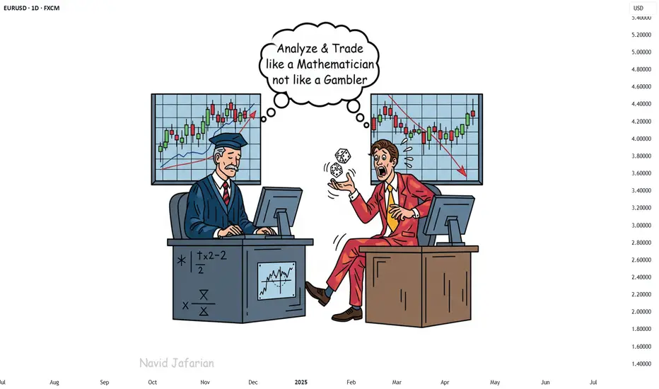
"Analyze with the precision of a mathematician and trade with the fighting spirit of a mathematician 👨🏻🎓,
not with the excitement of a gambler 🎲. "
Navid Jafarian
Every tip is a step towards becoming a more disciplined trader.
Look forward to the next one! 🌟
What Is T-Distribution in Trading? What Is T-Distribution in Trading?
In the financial markets, understanding T-distribution in probability is a valuable skill. This statistical concept, crucial for small sample sizes, offers insights into market trends and risks. By grasping T-distribution, traders gain a powerful tool for evaluating strategies, risks, and portfolios. Let's delve into what T-distribution is and how it's effectively used in the realm of trading.
Understanding T-Distribution
The T-distribution in probability distribution plays a crucial role in trading, especially in situations where sample sizes are small. William Sealy Gosset first introduced it under the pseudonym "Student". This distribution resembles the normal distribution with its bell-shaped curve but has thicker tails, meaning it predicts more outcomes in the extreme ends than a normal distribution would.
A key element of T-distribution is the concept of 'degrees of freedom', which essentially refers to the number of values in a calculation that are free to vary. It's usually the sample size minus one.
The degrees of freedom affect the shape of the T-distribution; with fewer degrees of freedom, the distribution has heavier tails. As the degrees of freedom increase, the distribution starts to resemble the normal distribution more closely. This is particularly significant in trading when dealing with small data sets, where the T-distribution provides a more accurate estimation of probability and risk than the normal distribution.
T-Distribution vs Normal Distribution
T-distribution and normal distribution are foundational in statistical analysis, yet they serve different purposes. While both exhibit a bell-shaped curve, the T-distribution has thicker tails, implying a higher probability of extreme values. This makes it more suitable for small sample sizes or when the standard deviation is unknown.
In contrast, the normal distribution, with its thinner tails, is ideal for larger sample sets where the standard deviation is known. Traders often use T-distribution for more accurate analysis in small-scale or uncertain data scenarios, while normal distribution is preferred for larger, more stable datasets, where extreme outcomes are less likely.
Application in Trading
In trading, T-distribution is a valuable tool for analysing financial data. It is primarily used in constructing confidence intervals and conducting hypothesis testing, which are essential for making informed trading decisions.
For instance, a trader might use T-distribution to test the effectiveness of a new trading strategy. Suppose a trader has developed a strategy using the technical analysis tools and wants to understand its potential effectiveness compared to the general market performance. They would collect a sample of returns from this strategy over a period, say, 30 days. Given the small sample size, using T-distribution is appropriate here.
The trader would then calculate the mean return of this sample and use T-distribution to create a confidence interval. This interval would provide a range within which the true mean return of the strategy is likely to lie, with a certain level of confidence. If this confidence interval shows a higher mean return than the market average, the trader might conclude that the strategy is potentially effective. However, it's important to note that this is an estimation and not a guarantee of future performance.
How to Plug Probability and Normal Distribution in Your T-Calculation
To use a T-calculator for integrating probability and normal distribution, follow these steps:
- Input Degrees of Freedom: For T-distribution, calculate the degrees of freedom (sample size minus one).
- Convert Z-Score to T-Value: If using normal distribution data, convert the Z-score (standard deviation units from the mean in a normal distribution) to a T-value using the formula: T = Z * (sqrt(n)), where 'n' is the sample size.
- Enter T-Value: Input this T-value into the calculator.
- Calculate Probability: The calculator will then output the probability, providing a statistical basis for trading decisions based on the T-distribution.
Limitations and Considerations of T-Distribution
While T-distribution is a powerful tool in trading analysis, it's important to recognise its limitations and considerations:
- Sample Size Sensitivity: T-distribution is most effective with small sample sizes. As the sample size increases, it converges to a normal distribution, reducing its distinct utility.
- Assumption of Normality: T-distribution assumes that the underlying data is approximately normally distributed. This may not hold true for all financial data sets, especially those with significant skewness or kurtosis.
- Degrees of Freedom Complications: Misestimating degrees of freedom can lead to inaccurate results. It's crucial to calculate this correctly based on the sample data.
- Outlier Sensitivity: T-distribution can be overly sensitive to outliers in the data, which can skew results.
Advanced Applications of T-Distribution in Trading
T-distribution extends beyond basic trading applications, playing a role in advanced financial analyses:
- Risk Modelling: Utilised in constructing sophisticated risk models, helping traders assess the probability of extreme losses.
- Algorithmic Trading: Integral in developing complex algorithms.
- Portfolio Optimisation: Assists in optimising portfolios by estimating returns and risks of various assets.
- Market Research: Used in advanced market research methodologies to analyse small sample behavioural studies.
The Bottom Line
The T-distribution is a powerful tool, offering nuanced insights in scenarios involving small sample sizes or uncertain standard deviations. Its ability to accommodate real-world data's quirks makes it invaluable for various trading applications, from strategy testing to risk assessment. However, understanding its limitations and proper application is crucial for accurate analysis.
This article represents the opinion of the Companies operating under the FXOpen brand only. It is not to be construed as an offer, solicitation, or recommendation with respect to products and services provided by the Companies operating under the FXOpen brand, nor is it to be considered financial advice.

Stop Hunting for Perfection - Start Managing Risk.Stop Hunting for Perfection — Start Managing Risk.
Hard truth:
Your obsession with perfect setups costs you money.
Markets don't reward perfectionists; they reward effective risk managers.
Here's why your perfect entry is killing your results:
You ignore good trades waiting for ideal setups — they rarely come.
You double-down on losing trades, convinced your entry was flawless.
You're blindsided by normal market moves because you didn’t plan for imperfection.
🎯 Solution?
Shift your focus from entry perfection to risk management. Define your maximum acceptable loss, stick to it, and scale into trades strategically.
TrendGo wasn't built to promise perfect entries. It was built to clarify probabilities and structure risk.
🔍 Stop chasing unicorns. Focus on managing the horses you actually ride.

Most Traders Want Certainty. The Best Ones Want Probability.Hard truth:
You’re trying to trade like an engineer in a casino.
You want certainty in an environment that only rewards probabilistic thinking.
Here’s how that kills your edge:
You wait for “confirmation” — and enter too late.
By the time it feels safe, the market has moved.
You fear losses — but they’re the cost of data.
Good traders don’t fear being wrong. They fear not knowing why.
You need to think in bets, not absolutes.
Outcomes don’t equal decisions. Losing on a great setup is still a good trade.
🎯 Fix it with better framing.
That’s exactly what we designed TrendGo f or — to help you see trend strength and structure without delusions of certainty.
Not perfect calls. Just cleaner probabilities.
🔍 Train your brain for the game you’re playing — or you’ll keep losing by default.

Probabilistic thinking. Using Technical logic to get odds.Markets are simple if you think about it.
moderate and long range resistance -- is the best odds for rally.
"horizontal" or 50-50 supports -- risky.
steep supports mean high demand, strong trends. Buying at such supports, at worst it bounces to the upside. (High market with strong trend can mean reversals)
rule: break outs always must coincide with 200dma rallies.
Bonus.
High market, strong trend -- best odds for reversal .
50-50 resistance, with weak support --> trickster market. (trap)
strong trend but no flying 200dma --> trap.
50-50 resistance with strong trend, high market, but weak 200dma ---> good odds for reversal.
keeping it simple.
P.S. this method shows why odds favor BTC reversal . Or why 110/120k had to be peak point. for now.

Trade high probabilities using game theoryAccording to statistics, 95% of traders are losing longterm. Not because they lack skill, but because they involve in high variance (or poor probability) situations.
What is game theory? we can define GT with three principles.
*People dont want to lose. (hence.. predictable).
*People buy good things at good price, or they are profit maximizing.
*Everyone is strategic.
** we assume that "nobody can predict future".
** markets respond to feedbacks or signals.
Practice: the higher something goes, potential narrows and risk increases. Deeper something falls, "potential" becomes attractive. Once market decides that it will fall -- people assume crash as possibility. People who can buy at a strong trend line - has benefit of having more information.
(1) Downtrending VIX highs and accumulating lows. a strong signal about SPX peak, with everyone expecting a market correction before US election. ---> GT in practice.
(2) pre-election. Markets be wobbly, pointing to 50-50 probability or risk. Maybe there was fear of NVDA/AAPL high valuations, or the fear due to Trump tariff policy (markets are 6m forward looking) as bond yields were rallying.
If we assume statistically, markets boom after elections. We can predict GT in action (or call it market forces). imo that still is a profitable risk.
People hate uncertainty and they love guarantees. So the "wobble" was reasonable.
(3) VIX higher low.. predictably (GT) sell off follows. Almost as by the book.
other way to put it? people maximize potential while minimize loses/risk. There are periods of volatile markets and periods for one directional rallies.
P.S. Blue arrows are longterm macd turning points.

ETCBTC is showing UPTHRUST , it can give better return over BTCreletivly etherium can give better return over bitcoin from this level..
invest 5% of your capital
risk /reward is very good
confidence intrade - High
this is not a financial advoice , just for educational purposes .

Reality & FibonacciParallels between Schrödinger’s wave function and Fibonacci ratios in financial markets
Just as the electron finds its position within the interference pattern, price respects Fibonacci levels due to their harmonic relationship with the market's fractal geometry.
Interference Pattern ⚖️ Fibonacci Ratios
In the double-slit experiment, particles including photons behave like a wave of probability, passing through slits and landing at specific points within the interference pattern . These points represent zones of higher probability where the electron is most likely to end up.
Interference Pattern (Schrodinger's Wave Function)
Similarly, Fractal-based Fibonacci ratios act as "nodes" or key zones where price is more likely to react.
Here’s the remarkable connection: the peaks and troughs of the interference pattern align with Fibonacci ratios, such as 0.236, 0.382, 0.618, 0.786. These ratios emerge naturally from the mathematics of the wave function, dividing the interference pattern into predictable zones. The ratios act as nodes of resonance, marking areas where probabilities are highest or lowest—mirroring how Fibonacci levels act in financial markets.
Application
In markets, price action often behaves like a wave of probabilities, oscillating between levels of support and resistance. Just as an electron in the interference pattern is more likely to land at specific points, price reacts at Fibonacci levels due to their harmonic relationship with the broader market structure.
This connection is why tools like Fibonacci retracements work so effectively:
Fibonacci ratios predict price levels just as they predict the high-probability zones in the wave function.
Timing: Market cycles follow wave-like behavior, with Fibonacci ratios dividing these cycles into phase zones.
Indicators used in illustrations:
Exponential Grid
Fibonacci Time Periods
Have you noticed Fibonacci ratios acting as critical levels in your trading? Share your insights in the comments below!

USDCAD H1 - Stress-Free Clear Charts.Stress-Free Clear Charts. (Required 10 years in R&D.)
In this layout, we see these indicators:
(From top to bottom of the screen)
-Angle: Shows the Angle of the Trend.
-Bear&Bull Powers: Displays who are in Power, the Bulls or the Bears.
-Strength: Shows the Strength of the Trend.
-Template: Always clearly shows the direction and precisely where to open and close (where to flip position). We open at the beginning of the Trend and stay in all the way till the end, stress-free. Turns perfectly.
-Performance: We see where to enter and close, the pullbacks and the performance.
-Odds: Shows the Odds everywhere.
-Probability: Shows the Probability all the way.
-Compare Forex: We see the performance of each currency of the Pair on chart. Each line is one currency. USD in Red. CAD in White. When the USD is above the CAD, the USDCAD pair goes up. And vice versa, when the USD is below the CAD, the USDCAD pair goes down. The background color displays the intensity of the trend.
