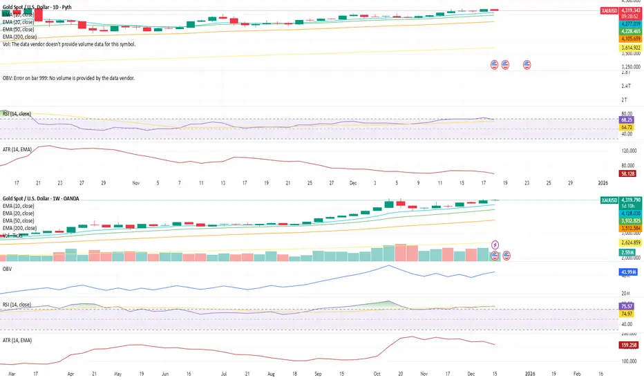
XAUUSD Structure Update — Daily & Weekly View1D Chart (Daily)
Gold continues to trade above all key EMAs, with the 10 EMA leading and holding steady, reinforcing short-term structural support rather than impulsive momentum.
RSI is taking a brief breather but remains elevated near 68, suggesting momentum is cooling in a controlled manner rather than breaking down.
ATR remains flat, indicating volatility is contained and price is progressing in an orderly fashion rather than expanding aggressively.
Due to the nature of spot gold volume, OBV on the daily timeframe is less informative, and participation signals are better assessed from the higher-timeframe structure.
Overall, the daily chart reflects consolidation within strength, not distribution.
1W Chart (Weekly)
The weekly structure continues to support the broader bullish framework.
Price remains above all major EMAs, with the 10 and 20 EMA rising steadily — not steep, but clearly directional — reinforcing sustainable trend progression rather than late-stage acceleration.
OBV trends higher on the weekly, signaling healthy participation and accumulation beneath the surface.
RSI holds near 75, elevated yet stable, indicating persistent strength without signs of exhaustion.
ATR remains flat, confirming that volatility remains controlled even as price holds elevated levels.
The weekly structure confirms that gold remains constructive and supported, with no technical evidence of breakdown.
⭐ Final Clarity Note ⭐
In structurally strong markets, consolidation often appears before continuation, not after failure.
When price holds above trend EMAs, volatility remains compressed, and participation persists on higher timeframes, it typically reflects positioning rather than speculation.
Gold’s current structure suggests the market is digesting gains, not abandoning them.
Risk!!!
Can Japan's Steel Giant Win the Green War?Nippon Steel Corporation stands at a critical crossroads, executing a radical transformation from domestic Japanese producer to global materials powerhouse. The company targets 100 million tons of global crude steel capacity under its "2030 Medium- to Long-term Management Plan," seeking 1 trillion yen in annual underlying business profit. However, this ambition collides with formidable obstacles: the politically contested $14.1 billion U.S. Steel acquisition faces bipartisan opposition despite Japan's allied status, while the strategic withdrawal from China, including dissolving a 20-year joint venture with Baosteel, signals a decisive "de-risking" pivot toward Western security frameworks.
The company's future hinges on its aggressive Indian expansion through the AM/NS India joint venture, which plans to triple capacity to 25-26 million tons by 2030, capturing the subcontinent's infrastructure boom and favorable demographics. Simultaneously, NSC is weaponizing its intellectual property dominance in electrical steel critical for EV motors through unprecedented patent litigation, even suing major customer Toyota to protect proprietary technology. This technological moat, exemplified by brands like "HILITECORE" and "NSafe-AUTOLite," positions NSC as an indispensable supplier in the global automotive lightweighting and electrification revolution.
Yet existential threats loom large. The "NSCarbolex" decarbonization strategy requires massive capital expenditures of 868 billion yen for electric arc furnaces alone, while bridging to unproven hydrogen direct reduction technology by 2050. Europe's Carbon Border Adjustment Mechanism threatens to tax NSC's exports into oblivion, forcing accelerated retirement of coal-based assets. The March 2025 cyberattack on subsidiary NSSOL exposed digital vulnerabilities as operational technology converges with IT systems. The NSC faces a strategic trilemma: balancing growth in protected markets, ensuring security through supply chain decoupling, and making sustainability investments that threaten near-term solvency. Success demands flawless execution across geopolitical, technological, and financial dimensions, simultaneously a precarious bet on reshaping the global steel order.

How AI is Revolutionizing Risk ManagementIn a world where bots can fire off hundreds of orders in the time it takes you to sip your coffee, risk management isn't a checkbox at the end of your plan it's the core operating system.
AI has given traders incredible leverage:
Faster execution than any human
Exposure to more markets and instruments
Complex position structures that would be impossible to manage manually
But that same leverage cuts both ways. When something breaks, it doesn't trickle it cascades.
The traders who survive this era won't be the ones with the most aggressive models. They'll be the ones whose risk frameworks are built to handle both human mistakes and machine speed.
Why Old-School Risk Rules Aren't Enough Anymore
For years, the standard advice looked like this:
"Never risk more than 1–2% per trade"
"Always use a stop loss"
"Diversify across assets"
Those principles still matter so much. But AI and automation helped improve and changed the landscape:
Orders can hit the market in microseconds your "mental stop" is useless
Correlations spike during stress what looked diversified suddenly moves as one
Multiple bots can unintentionally stack risk in the same direction
Feedback loops between algos can turn a normal move into a cascade
In other words: the classic rules are the starting point , not the full playbook.
How AI Supercharges Risk Management (If You Let It)
Used well, AI doesn't just place trades it monitors and defends your account in ways a human never could.
Dynamic Position Sizing
Instead of risking a flat 1% on every trade, AI can adjust size based on:
Current volatility
Recent strategy performance
Correlation with existing positions
Market regime (trend, range, chaos)
When conditions are favorable, size can step up modestly.
When conditions are hostile, size automatically steps down.
The goal isn't to swing for home runs.
It's to press when the wind is at your back, and survive when it's in your face.
Smarter Stop Placement
Fixed stops at round numbers are magnets for liquidity hunts.
AI can analyze:
ATR-based volatility bands
Clusters of swing highs/lows
Liquidity pockets in the book
Option levels where hedging flows are likely
Stops get placed where the idea is broken, not where noise usually spikes.
Portfolio-Level Heat Monitoring
Most traders think in single trades. AI thinks in portfolios.
It can continuously measure:
Total percentage of equity at risk right now
Sector and theme concentration
Correlation clusters (everything tied to the same macro factor)
Worst-case scenarios under shock moves
If your "independent" trades are all secretly the same bet, a good risk engine will tell you.
The 4-Layer Risk Stack for AI Traders
Think of your protection as layered armor:
Trade Level
Clear stop loss
Defined target or exit logic
Position size tied to account risk, not feelings
Strategy Level
Max number of open positions per strategy
Daily loss limit per system
"Three strikes" rules after consecutive losing days
Portfolio Level
Total open risk cap (for example: no more than 2% at risk at once)
Limits by asset class, sector, and narrative
Rules to prevent over concentration in one theme (AI stocks, crypto, etc.)
Account Level
Maximum drawdown you're willing to tolerate
Hard kill switch when that line is crossed
Recovery plan (size reductions, pause period, review process)
AI can monitor all four layers at once every position, every second and trigger actions the moment a rule is violated.
Kelly, Edge, and Why "More" Is Not Always Better
The Kelly Criterion is a famous formula that tells you how much of your account you could risk to maximize long‑term growth.
Kelly % = W - ((1 - W) / R)
Where:
W = Win probability
R = Average Win / Average Loss
Example:
Win rate (W) = 60%
Average win is 1.5× average loss (R = 1.5)
Kelly = 0.60 - (0.40 / 1.5) ≈ 0.33 → 33%
On paper, that says "risk 33% of your account each trade." In reality, that's a fast path to a margin call.
Serious traders and any sane AI risk engine treat Kelly as the ceiling , then scale it down:
Half‑Kelly (≈ 16%)
Quarter‑Kelly (≈ 8%)
Or even less, depending on volatility and confidence
AI can recompute W and R as fresh trades come in, adjusting risk when your edge is hot and cutting risk when your edge is questionable.
Designing Your AI‑Era Risk Framework
You don't need hedge‑fund infrastructure to think like a pro. Start with five questions:
What is my absolute pain threshold?
At what drawdown (%) would I stop trading entirely?
Write that number down. Build backwards from it.
How many consecutive losses can I survive?
If you want to survive 10 straight losses at 20% max drawdown, your per‑trade risk must be ~2% or less.
How will I shrink risk when volatility spikes?
Tie your size to ATR, VIX‑style measures, or your own volatility index.
What are my circuit breakers?
Daily loss limit
Weekly loss review trigger
Conditions where all bots shut down automatically
Is everything written down?
If it's not in rules, it's just a wish.
Rules should be clear enough that a bot could follow them.
Four AI Risk Mistakes That Blow Accounts Quietly
Over‑optimization - Training models until the backtest is perfect… and live trading is a disaster.
Ignoring tail risk - Assuming the future will look like the backtest, and underestimating rare events.
No true kill switch - Letting a "temporary" drawdown turn into permanent damage.
Blind trust in the model - Assuming "the bot knows best" without understanding its logic.
AI should be treated like a high‑performance car: powerful, fast, and absolutely deadly if you drive it without brakes.
Discussion
How are you handling risk in the age of automation?
Do you size positions dynamically or use fixed percentages?
Do you cap total portfolio risk, or just think trade by trade?
Do your bots or strategies have clear kill switches?
Drop your thoughts and your best risk rules in the comments. In the future of trading AI will be the one watching your back.....
Can One Company Own the Ocean Floor?Kraken Robotics has emerged as a dominant force in subsea intelligence, riding three converging megatrends: the weaponization of seabed infrastructure, the global energy transition to offshore wind, and the technological obsolescence of legacy sonar systems. The company's Synthetic Aperture Sonar (SAS) technology delivers range-independent 3cm resolution, 15 times superior to conventional systems. At the same time, its pressure-tolerant SeaPower batteries solve the endurance bottleneck that has plagued autonomous underwater vehicles for decades. This technological moat, protected by 31 granted patents across 19 families, has transformed Kraken from a niche sensor manufacturer into a vertically integrated subsea intelligence platform.
The financial metamorphosis validates this strategic positioning. Q3 2025 revenue surged 60% Year-Over-Year to $31.3 million, with gross margins expanding to 59% and adjusted EBITDA growing 92% to $8.0 million. The balance sheet fortress of $126.6 million in cash, up 750% from the prior year, provides the capital to pursue a dual strategy: organic growth through NATO's Critical Undersea Infrastructure initiative and strategic acquisitions, such as the $17 million purchase of 3D at Depth, which added subsea LiDAR capabilities. The market's 1,000% re-rating since 2023 reflects not speculative excess but a fundamental recognition that Kraken controls critical infrastructure for the emerging blue economy.
Geopolitical tensions have accelerated demand, with the Nord Stream sabotage serving as an inflection point for defense procurement. NATO's Baltic Sentry mission and the alliance-wide focus on protecting 97% of internet traffic carried by undersea cables create sustained tailwinds. Kraken's technology participated in seven naval teams at REPMUS 2025, demonstrating platform-agnostic interoperability that positions it as the universal standard. Combined with exposure to the offshore wind supercycle (250 GW by 2030) and potential deep-sea mining operations valued at $177 trillion in resources, Kraken has positioned itself as the indispensable "picks and shovels" provider for multiple secular growth vectors simultaneously.

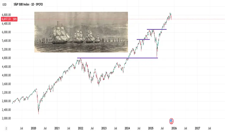
Old Ship Fleet: uncertainty and risk.In the old days, buying a trading ship posed risks due to natural disasters. Later on, people could have option to buy lets say a 10% share in a fleet of 10 trading ships. When one ship goes down, it doesn't ruin your "portfolio".
I think the concept about not putting all eggs in one basket fits well into risk taking.
Then you have some investors claim, you put all your eggs into one basket - and guard the basket.
The ship fleet works as a syllogism about uncertainty. Math (probability of disaster on statistical basis). And risk taking.
Eggs in one basket is a syllogism about losing everything. But not uncertainty or risk-taking per se.
-> In competitive spaces, with only few or one winner. With exponential, explosive returns -- diversifying or putting eggs in separate baskets make no sense. "Fortune favors the bald" is a better way to describe it.
but it says nothing about mathematical side of uncertainty or risk taking. Hence the "old ship fleet".
The Dual Catalyst: Why Silver's \$50 Breakout is SustainableSilver (XAG/USD) recently broke the crucial $50 per ounce level, signaling a fundamental shift in its market dynamics. While the price edges lower in the short term, primarily due to a strengthened US Dollar (USD), its long-term trajectory is decisively bullish. This surge is not merely speculative. It is driven by an unprecedented convergence of geopolitical risks, critical industrial demand, and shifting macroeconomic policy. Analyzing these catalysts across multiple domains confirms silver's evolving role from a precious metal to a critical industrial asset.
Macroeconomics and Geopolitics
Silver's price strength reflects global systemic risk and monetary policy uncertainty. Current market expectations strongly favor a Federal Reserve (Fed) rate cut by December, with a nearly 68% probability priced in by the CME FedWatch Tool. Lower interest rates reduce the opportunity cost of holding non-yielding silver, making it relatively more attractive than bonds or cash. This dovish outlook provides a powerful structural floor for the price.
From a geopolitical perspective, ongoing global tensions and elevated political risks, like recent US government funding debates, accelerate safe-haven demand. Investors seek hard assets to hedge systemic risks. While gold often leads as the primary safe haven, silver's lower cost and dual-use nature attract broader retail and institutional flows, pushing it higher. A strong, sustained rally will require the price to hold above $50 and overcome the next major resistance near the historical high of $54.50.
Technology, Science, and Patents
Industrial demand now constitutes over 50% of silver’s total annual consumption, fundamentally redefining its market. Its unmatched electrical and thermal conductivity makes it indispensable in high-growth sectors.
* Renewable Energy: Silver is critical for photovoltaics (PV), specifically in solar cells, which form the conductive paste that harvests electrons. The global push for green energy and solar capacity expansion creates structural, persistent demand that consistently tightens the market.
* High-Tech and EVs: Electric Vehicles ( EVs) require significantly more silver (25–50 grams per unit) than traditional vehicles for inverters, battery management systems, and high-voltage contacts. The expansion of 5G technology, advanced computing, and the Internet of Things (IoT) further relies on silver-based components for seamless connectivity and efficiency.
Geostrategy and Supply Chain Risk
Silver is now recognized as a critical mineral by several major economies. This reclassification acknowledges its essential role in national security, advanced manufacturing, and the energy transition. This status highlights a geopolitical vulnerability: silver's supply chain is increasingly seen as a strategic concern.
The market currently runs a persistent supply deficit, depleting above-ground stockpiles to critically low levels. Mining silver often occurs as a byproduct of copper, lead, and zinc, meaning its supply cannot easily scale up based on price alone. Trade conflicts or export controls imposed by major producing nations could severely disrupt supply, immediately spiking the price due to its non-substitutable role in key high-tech applications.
Cyber and Economics: The Future Nexus
Silver’s unique properties extend into emerging fields like cybersecurity* and advanced computing. Research integrates silver nanoparticles and quantum materials into sophisticated systems. These materials enhance data processing efficiency and bolster the security of financial supply chains. Furthermore, flexible electronics using silver nanowires* will drive the next generation of wearable and flexible displays, creating entirely new demand vectors.
The long-term economic case for a $100 silver price remains dependent on this confluence of factors. Sustained high industrial consumption, a breakdown in global supply chains, and a continued environment of monetary debasement must align. Silver has truly become a dual-catalyst metal, positioned to thrive as both a financial safe haven and a fundamental building block of the twenty-first-century green and digital economy.

Is Germany's Economic Success Just an Illusion?Germany's benchmark DAX 40 index surged 30% over the past year, creating an impression of robust economic health. However, this performance masks a troubling reality: the index represents globally diversified multinationals whose revenues originate largely outside Germany's struggling domestic market. Behind the DAX's resilience lies fundamental decay. GDP fell 0.3% in Q2 2025, industrial output reached its lowest level since May 2020, and manufacturing declined 4.8% year-over-year. The energy-intensive sector suffered even steeper contraction at 7.5%, revealing that high input costs have become a structural, long-term threat rather than a temporary challenge.
The automotive sector exemplifies Germany's deeper crisis. Once-dominant manufacturers are losing ground in the electric vehicle transition, with their European market share in China plummeting from 24% in 2020 to just 15% in 2024. Despite leading global R&D spending at €58.4 billion in 2023, German automakers remain trapped at Level 2+ autonomy while competitors pursue full self-driving solutions. This technological lag stems from stringent regulations, complex approval processes, and critical dependencies on Chinese rare earth materials, which could trigger €45-75 billion in losses and jeopardize 1.2 million jobs.
Germany's structural rigidities compound these challenges. Federal fragmentation across 16 states paralyzes digitalization efforts, with the country ranking below the EU average in digital infrastructure despite ambitious sovereignty initiatives. The nation serves as Europe's fiscal anchor, contributing €18 billion net to the EU budget in 2024, yet this burden constrains domestic investment capacity. Meanwhile, demographic pressures persist, though immigration has stabilized the workforce; highly skilled migrants disproportionately consider leaving, threatening to transform a demographic solution into brain drain. Without radical reform to streamline bureaucracy, pivot R&D toward disruptive technologies, and retain top talent, the disconnect between the DAX and Germany's foundational economy will only widen.

Halloween Special: The Risk “Treats” That Keep You Alive!🧠 If October has a lesson, it’s this: fear is useful, panic is fatal. Great traders don’t fight the monsters; they contain them.
Here’s my Halloween mindset & risk playbook:
🧪 Keep your “lifeline” small: Risk a fixed 1% per trade until your balance moves ±10%, then recalibrate. This makes loss streaks survivable and hot streaks meaningful.
⏰ Set a nightly curfew: a max daily loss (e.g., 3R or 3%). Hit it? Close the platform. No “one last trade.” Curfews save accounts.
🛑 Define your invalidation before you enter: If that level prints, you’re out, no arguments, no “maybe it comes back.” Plans beat feelings.
🎯 Hunt asymmetry: If you can’t see at least 2R cleanly (preferably 3R), pass. You don’t need more trades; you need better trades.
🧟 Kill the zombie trade: the one you’re babysitting, nudging stops, praying. If you’re managing hope more than risk, exit and reset.
🧘 Protect your mind equity: Two back-to-back losses? Take a 20-minute break. After a big win? Journal before you click again. Calmness compounds.
📜 Make a ritual: pre-trade checklist → position size → entry → stop → targets → log. Rituals turn uncertainty into routine, and routine into consistency.
What’s your #1 rule that keeps the “revenge-trading demon” out of your account❓
⚠️ Disclaimer: This is not financial advice. Always do your own research and manage risk properly.
📚 Stick to your trading plan regarding entries, risk, and management.
Good luck!
All Strategies Are Good; If Managed Properly!
~Richard Nasr

Position Sizing: The Math That Separates Winners from LosersMost traders blow up their accounts not because of bad entries, but because of terrible position sizing. You can have a 60% win rate and still go broke if you risk too much per trade.
The 1-2% Rule (And Why It Works)
Never risk more than 1-2% of your account on a single trade.
Here's why this matters:
Risk 2% per trade → You can survive 50 consecutive losses
Risk 10% per trade → 10 losses = -65% drawdown (you need +186% just to break even)
Risk 20% per trade → 5 losses = game over
The Position Sizing Formula
Position Size = (Account Size × Risk %) / (Entry Price - Stop Loss)
Real Example:
Account: $10,000
Risk per trade: 2% = $200
Entry: $50
Stop loss: $48
Risk per share: $2
Position Size = $200 / $2 = 100 shares
If stopped out → You lose exactly $200 (2%)
If price hits $54 → You make $400 (4% gain, 2:1 R/R)
Different Risk Frameworks
Conservative (1% risk)
Best for: Beginners, volatile markets, high-frequency trading
Survivability: Can take 100+ losses
Growth: Slower but steady
Moderate (2% risk)
Best for: Experienced traders, tested strategies
Survivability: 50 consecutive losses
Growth: Balanced risk/reward
Aggressive (3-5% risk)
Best for: High conviction setups, smaller accounts trying to grow
Survivability: 20-33 losses
Growth: Faster but dangerous
Warning: Never go above 5% unless you're gambling, not trading.
The Kelly Criterion (Advanced)
For traders with significant backtested data:
Kelly % = Win Rate -
Example:
Win rate: 55%
Avg win: $300
Avg loss: $200
Win/Loss ratio: 1.5
Kelly % = 0.55 - = 0.55 - 0.30 = 25%
But use 1/4 Kelly (6.25%) or 1/2 Kelly (12.5%) - Full Kelly is too aggressive for real markets.
Common Position Sizing Mistakes
❌ Revenge trading larger after a loss
✅ Keep position size constant based on current account value
❌ Risking the same dollar amount regardless of setup quality
✅ Risk 0.5% on B-setups, 2% on A+ setups
❌ Ignoring correlation risk
✅ If you have 5 tech stocks open, you're really risking 10% on one sector
❌ Not adjusting after drawdowns
✅ If account drops 20%, your 2% risk should recalculate from new balance
The Volatility Adjustment
In high volatility (VIX > 30):
Cut position sizes by 30-50%
Widen stops or risk less per trade
Market can gap past your stops
In low volatility (VIX < 15):
Can use normal position sizing
Tighter stops possible
More predictable price action
My Personal Framework
I use a tiered approach:
High conviction setups (A+): 2% risk
Good setups (A): 1.5% risk
Decent setups (B): 1% risk
Experimental/learning: 0.5% risk
Maximum combined risk: Never more than 6% across all open positions.
The Bottom Line
Position sizing is the only thing you have complete control over in trading. You can't control:
Where price goes
Market volatility
News events
But you CAN control how much you risk.
The traders who survive long enough to get good are the ones who master position sizing first.
What's your current risk per trade? Drop it in the comments. If it's above 5%, we need to talk.
Can Defense Giants Print Money During Global Chaos?General Dynamics delivered exceptional Q3 2025 results with revenue reaching $12.9 billion (up 10.6% year-over-year) and diluted EPS soaring to $3.88 (up 15.8%). The company's dual-engine growth strategy continues to drive performance: its defense segments capitalize on mandatory global rearmament driven by escalating geopolitical tensions, while Gulfstream Aerospace leverages resilient demand from high-net-worth individuals. The Aerospace segment alone grew revenue by 30.3% with operating margin expanding 100 basis points, delivering record jet deliveries as supply chains normalized. Operating margin reached 10.3% overall, with operating cash flow hitting $2.1 billion—an extraordinary 199% of net earnings.
The defense portfolio secures decades of revenue visibility through strategic programs, most notably the $130 billion Columbia-class submarine program, which represents the U.S. Navy's top acquisition priority. General Dynamics European Land Systems has secured a €3 billion contract from Germany for next-generation reconnaissance vehicles, capitalizing on record European defense spending that reached €343 billion in 2024 and is projected to reach €381 billion in 2025. The Technology division strengthened its position with $2.75 billion in recent IT modernization contracts, deploying AI, machine learning, and advanced cybersecurity capabilities for critical military infrastructure. The company's 3,340-patent portfolio, with over 45% still active, reinforces its competitive moat in nuclear propulsion, autonomous systems, and signals intelligence.
However, significant operational headwinds persist in the Naval segment. The Columbia-class program faces a 12-to 16-month delay, with the first delivery now anticipated between late 2028 and early 2029, driven by supply chain fragility and specialized workforce shortages. Late delivery of major components forces complex out-of-sequence construction work, while the defense industrial base struggles with critical skill gaps in nuclear-certified welders and specialized engineers. Management emphasizes that the upcoming year will be pivotal for driving productivity improvements and margin recovery in Naval operations.
Despite near-term challenges, General Dynamics' balanced portfolio positions it for sustained outperformance. The combination of non-discretionary defense spending, technological superiority in strategic systems, and robust free cash flow generation provides resilience against volatility. Success in stabilizing the submarine industrial base will determine long-term margin trajectory, but the company's strategic depth and cash generation capability support continued alpha generation in an increasingly uncertain global environment.

Patience - When Calm Feels WrongNOTE – This is a post on mindset and emotion. It is not a trade idea or strategy designed to make you money. My intention is to help you preserve your capital, focus, and composure — so you can trade your own system with calm and confidence.
Markets quiet down.
Price moves slow.
Everything looks still, maybe too still.
Part of you relaxes.
Another part tenses.
It’s that sense that something’s coming.
And sometimes, it is.
But here’s the hard part
Your body doesn’t always know the difference between anticipating danger and feeling unsafe.
For traders, the nervous system reads uncertainty like threat.
Even a normal pause in volatility can trigger the same internal siren:
Something’s wrong. Do something.
You start scanning: news, charts, signals
anything to justify the unease.
But often, the danger isn’t out there.
It’s inside you... a learned association between stillness and not knowing what's going to happen next
Which causes restlessness, uncertainty and a need to fidget and meddle.
The skill isn’t in shutting that instinctive unease down.
It’s in listening without reacting impulsively.
Ask yourself - what is really going on right here, right now?
The point here is:
Patience isn’t passive.
It’s regulated awareness.
It’s being alert, not alarmed.
Ready, but not restless.
Sometimes there is indeed a risk out there.
We are trading the financial markets after all.
However. You have a trading plan.
You know to be risk measured.
All that is needed now is the ability to regulate yourself
Stay calm and patient so you can execute your plan as intended.

Trading Crude Oil and the Geopolitical Impact on PricesIntroduction
Crude oil is one of the most strategically significant commodities in the global economy. It fuels transportation, powers industries, and serves as a critical input for countless products ranging from plastics to fertilizers. Because of its universal importance, crude oil trading is not just a financial endeavor—it is a reflection of global political stability, economic growth, and international relations. The price of crude oil is highly sensitive to geopolitical events, including wars, sanctions, alliances, and policy changes. Understanding how geopolitical dynamics affect oil trading and pricing is vital for traders, investors, and policymakers.
1. The Fundamentals of Crude Oil Trading
Crude oil trading involves the buying and selling of oil in various markets, primarily through futures contracts on exchanges such as the New York Mercantile Exchange (NYMEX), Intercontinental Exchange (ICE), and Dubai Mercantile Exchange (DME). These contracts allow traders to speculate on the future price of oil, hedge against risks, or facilitate physical delivery. Two main benchmark grades dominate the market: West Texas Intermediate (WTI) and Brent Crude.
WTI Crude Oil is primarily sourced from the U.S. and traded in dollars per barrel.
Brent Crude Oil is produced in the North Sea and serves as the global benchmark for pricing.
Oil prices are influenced by multiple factors, including supply and demand fundamentals, global economic growth, production levels, inventory data, transportation costs, and geopolitical events. Among these, geopolitical tensions often have the most immediate and dramatic impact.
2. Geopolitics as a Determinant of Oil Prices
The global oil market is uniquely vulnerable to geopolitical developments because a significant portion of reserves and production is concentrated in politically sensitive regions such as the Middle East, North Africa, and Russia. Around 60% of proven oil reserves lie in OPEC (Organization of Petroleum Exporting Countries) member nations, many of which have experienced conflict, sanctions, or regime instability.
Geopolitical risk refers to the potential disruption in oil supply or transportation routes due to international conflicts, political upheaval, or policy decisions. When such risks escalate, traders often bid up oil prices in anticipation of supply shortages—even before any actual disruption occurs.
3. Historical Perspective: Major Geopolitical Events and Oil Prices
a. The 1973 Arab Oil Embargo
One of the earliest and most significant examples of geopolitically driven oil price shocks occurred in 1973 when Arab OPEC members imposed an oil embargo against the United States and other nations supporting Israel during the Yom Kippur War. Oil prices quadrupled within months, leading to inflation, recession, and a global energy crisis. The embargo demonstrated the power of oil as a political weapon and the vulnerability of consumer nations.
b. The Iranian Revolution (1979)
The overthrow of the Shah of Iran and the subsequent decline in Iranian oil production reduced global supply by nearly 5%. This shortage, coupled with the Iran-Iraq War (1980–1988), sent prices soaring again. The resulting volatility highlighted how political instability in a single oil-producing nation could ripple through the entire global economy.
c. The Gulf War (1990–1991)
Iraq’s invasion of Kuwait disrupted nearly 5 million barrels per day of oil production. The U.S.-led coalition’s response and the ensuing war created massive uncertainty in the Middle East, briefly pushing oil prices above $40 per barrel—a significant level for that time.
d. The Iraq War (2003)
The U.S. invasion of Iraq reignited geopolitical fears about supply disruptions. Although global production eventually stabilized, the war contributed to sustained higher oil prices in the early 2000s, further compounded by rapid industrialization in China and India.
e. The Arab Spring (2010–2011)
The wave of protests across the Middle East and North Africa led to regime changes and unrest in key producers such as Libya and Egypt. The civil war in Libya, in particular, cut oil output by over one million barrels per day, causing Brent crude prices to exceed $120 per barrel.
f. Russia-Ukraine Conflict (2014 and 2022)
Russia’s annexation of Crimea in 2014 and its full-scale invasion of Ukraine in 2022 significantly disrupted global energy markets. As one of the world’s largest oil and gas exporters, Russia faced Western sanctions that restricted exports, insurance, and financing. In early 2022, Brent crude spiked above $130 per barrel, reflecting fears of prolonged supply shortages and energy insecurity across Europe.
4. Channels Through Which Geopolitics Impacts Oil Prices
Geopolitical events influence oil prices through several interconnected channels:
a. Supply Disruptions
Conflicts or sanctions can directly reduce oil supply by damaging infrastructure, limiting production, or restricting exports. For example, sanctions on Iran in 2012 and again in 2018 led to significant declines in its oil exports, tightening global supply.
b. Transportation and Shipping Risks
Chokepoints such as the Strait of Hormuz, Suez Canal, and Bab el-Mandeb Strait are vital for global oil transportation. Any military conflict or threat in these areas immediately raises concerns about shipping disruptions, leading to higher prices. Nearly 20% of global oil passes through the Strait of Hormuz daily.
c. Speculative Reactions
Traders and hedge funds respond quickly to geopolitical news, often amplifying price movements. Futures markets price in expected risks, causing volatility even when actual supply remains unaffected.
d. Strategic Reserves and Policy Responses
Nations often release oil from strategic reserves or negotiate production increases through OPEC to stabilize markets. For example, the U.S. and IEA (International Energy Agency) coordinated strategic reserve releases in 2022 to offset supply disruptions caused by the Russia-Ukraine conflict.
e. Currency Movements
Since oil is traded in U.S. dollars, geopolitical tensions that weaken the dollar or create global uncertainty can influence oil prices. A weaker dollar often makes oil cheaper for non-U.S. buyers, boosting demand and raising prices.
5. OPEC and Geopolitical Strategy
The Organization of Petroleum Exporting Countries (OPEC), formed in 1960, and its extended alliance OPEC+, which includes Russia, play a pivotal role in determining oil supply and prices. The organization uses coordinated production quotas to manage global prices, often aligning decisions with geopolitical interests.
For instance:
In 2020, during the COVID-19 pandemic, OPEC+ cut production by nearly 10 million barrels per day to support collapsing prices.
In 2023, Saudi Arabia and Russia announced voluntary cuts to maintain price stability amid slowing demand and Western sanctions.
OPEC’s policies are inherently geopolitical, balancing the economic needs of producers with the political relationships among member states and major consumer nations.
6. Energy Transition and the New Geopolitics of Oil
The growing global emphasis on renewable energy and decarbonization is reshaping the geopolitical landscape of oil trading. As nations transition to cleaner energy, oil-producing countries face the challenge of maintaining revenue while managing political stability.
However, this transition also introduces new geopolitical dependencies—for example, on lithium, cobalt, and rare earth metals used in electric vehicle batteries. While demand for oil may gradually plateau, geopolitical risks remain as nations compete over new energy supply chains.
Additionally, U.S. shale production has transformed the country from a net importer to a major exporter, reducing its vulnerability to Middle Eastern geopolitics but also introducing new market dynamics. Shale producers can ramp up or scale down production relatively quickly, acting as a “shock absorber” to global price swings.
7. The Role of Technology and Market Transparency
Technological advancements in trading—especially algorithmic and data-driven models—have increased market liquidity but also heightened sensitivity to news. Real-time tracking of geopolitical developments via satellites, social media, and analytics platforms allows traders to react instantly.
For example, satellite data showing tanker movements or refinery fires can trigger immediate price adjustments. The intersection of AI, big data, and geopolitics now defines modern oil trading strategies, with traders assessing both quantitative signals and qualitative geopolitical intelligence.
8. Managing Geopolitical Risk in Oil Trading
Professional oil traders and corporations employ various strategies to manage geopolitical risks:
Diversification: Sourcing oil from multiple regions to minimize reliance on unstable producers.
Hedging: Using futures, options, and swaps to lock in prices and reduce exposure to volatility.
Scenario Analysis: Running stress tests based on potential geopolitical outcomes (e.g., war, sanctions, embargoes).
Political Risk Insurance: Protecting investments against losses due to government actions or conflict.
Strategic Reserves: Governments maintain emergency stockpiles to stabilize supply during crises.
In addition, diplomatic engagement and international cooperation—such as IEA coordination or U.N.-mediated negotiations—can help mitigate disruptions and maintain market balance.
9. The Future Outlook: Geopolitics and the Oil Market
As of the mid-2020s, the global oil market faces a new era of geopolitical uncertainty. Key issues shaping the future include:
The U.S.-China rivalry, which may influence energy trade routes and technological access.
Middle Eastern realignments, including normalization of relations between former rivals and shifting alliances.
Climate policy conflicts, as nations balance carbon reduction commitments with economic growth needs.
Sanctions regimes on Russia, Iran, and Venezuela, which continue to restrict global supply flexibility.
The digitalization of trading, which increases speed and transparency but also amplifies volatility.
Although long-term demand growth may slow due to renewable energy adoption, oil will remain a central geopolitical and economic asset for decades. The world’s dependence on energy ensures that geopolitics will continue to shape price trends, investment decisions, and market psychology.
Conclusion
Crude oil trading is not merely a reflection of supply and demand; it is a barometer of global stability and geopolitical tension. From the 1973 oil embargo to the ongoing Russia-Ukraine conflict, political decisions have repeatedly proven capable of reshaping energy markets. For traders and policymakers alike, understanding the geopolitical dimensions of oil is crucial for navigating price volatility and maintaining economic resilience.
As the energy transition accelerates, the nature of geopolitical risk will evolve—but it will not disappear. The intersection of oil, politics, and global economics will continue to define international relations and financial markets, ensuring that crude oil remains one of the world’s most geopolitically sensitive and closely watched commodities.

HOW to USE OB After Liq sweept on daily bais CME_MINI:MNQ1!
After we took PDL we Choch on 1H
and 5 min ob appear for more push

Position Sizing and Risk ManagementThere are multiple ways to approach position sizing. The most suitable method depends on the trader’s objectives, timeframe, and account structure. For example, a long-term investor managing a portfolio will operate differently than a short-term trader running a high-frequency system. This chapter will not attempt to cover all possible methods, but will focus on the framework most relevant to the active trader.
Equalized Risk
The most practical method for position sizing is known as equalized risk per trade. This model ensures that each trade risks the same monetary amount, regardless of the stop loss distance. The position size will be calculated based on the distance between the entry price and the stop loss, which means a closer stop equals more size, where a wider stop equals less size. This allows for a more structured and consistent risk control across various events.
Position Size = Dollar Risk / (Entry Price − Stop Price)
Position Size = Dollar Risk / (Entry Price × Stop in %)
For example, an account size of $100,000 and risk amount of 1% will be equivalent to $1,000. In the scenario of a $100 stock price, the table below provides a visual representation of how the position size adapts to different stop loss placements, to maintain an equalized risk per trade. This process can be integrated into order execution on some trading platforms.
The amount risked per trade should be based on a fixed percentage of the current account size. As the account grows, the dollar amount risked increases, allowing for compounding. If the account shrinks, the dollar risk decreases, which helps reduce the impact of continued losses. This approach smooths out the effect of random sequences. A percentage-based model limits downside exposure while preserving upside potential.
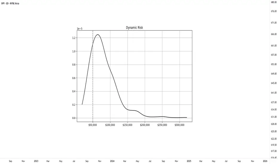
To better illustrate how position sizing affects long-term outcomes, a controlled simulation was conducted. The experiment modeled a system with a 50% win rate and a 1.1 to 1 average reward-to-risk ratio. Starting with a $50,000 account, the system executed 500 trades across 1000 separate runs. Two position sizing methods were compared: a fixed dollar risk of $1000 per trade and a dynamic model risking 2% of the current account balance.
Fixed-Risk Model
In the fixed-risk model, position size remained constant throughout the simulation. The final outcomes formed a relatively tight, symmetrical distribution centered around the expected value, which corresponds to consistent variance.
Dynamic-Risk Model
The dynamic-risk model produced a wider and more skewed distribution. Profitable runs experienced accelerated increase through compounding, while losing runs saw smaller drawdowns due to self-limiting trade size. Although dynamic risk introduces greater dispersion in final outcomes, it allows scalable growth over time. This compounding effect is what makes a dynamic model effective for achieving exponential returns.
A common question is what percentage to use. A range between 1–3% of the account is generally considered reasonable. Too much risk per trade can quickly become destructive, consider that even profitable systems may experience a streak of losses. For instance, a series of five consecutive losses at 10% risk per trade would cut the account by roughly 41%, requiring over a 70% return to recover. In case catastrophic events occur; large position sizing makes them irreversible. However, keeping position size and risk too small can make the entire effort unproductive. There is no such thing as a free trade, meaningful reward requires exposure to risk.
Risk Definition and Stop Placement
Risk in trading represents uncertainty in both the direction and magnitude of outcomes. It can be thought of as the potential result of an event, multiplied by the likelihood of that event occurring. This concept can be formulated as:
Risk = Outcome × Probability of Outcome
This challenges a common assumption that using a closer stop placement equals reduced risk. This is a common misconception. A tighter stop increases the chance of being triggered by normal price fluctuations, which can result in a higher frequency of losses even when the trade idea is valid.
Wide stop placements reduce the likelihood of premature exit, but they also require price to travel further to reach the target, which can slow down the trade and distort the reward-to-risk profile. An effective stop should reflect the volatility of the instrument while remaining consistent with the structure of the setup. A practical guideline is to place stops within 1–3 times the ATR, which allows room for price movement without compromising the reward-risk profile.
When a stop is defined, the distance from entry to stop becomes the risk unit, commonly referred to as R. A target placed at the same distance above the entry is considered 1R, while a target twice as far is 2R, and so on. Thinking in terms of R-multiples standardizes evaluation across different instruments and account sizes. It also helps track expectancy, maintain consistency, and compare trading performance.
In summary, risk is best understood as uncertainty, where the outcome is shaped by both the possible result and the probability of it occurring. The preferred approach for the active trader is equalized risk per trade, where a consistent percentage of the account, typically 1–3%, is risked on each position regardless of the stop distance. This allows the account to develop through compounding. It also reinforces the importance of thinking in terms of sample size. Individual trades are random, but consistent risk control allows statistical edge to develop over time.
Practical Application
To simplify this process, the Risk Module has been developed. The indicator provides a visual reference for position sizing, stop placement, and target definition directly on the chart. It calculates equalized risk per trade and helps maintain consistent exposure.
TRADING LEVERAGE | How to Manage RISK vs REWARDFor today's post, we're diving into the concept " Risk-Reward Ratio "
We'll take a look at practical examples and including other relevant scenarios of managing your risk. What is considered a good risk to reward ratio and where can you see it ? This applies to all markets, and during these volatile times it is an excellent idea to take a good look at your strategy and refine your risk management.
You've all noticed the really helpful tool " long setup " or " short setup " on the left-hand column. This clearly identifies the area of profit (in green), the area for a stop-loss (in red) and your entry (the borderline). It also shows the percentage of your increases or decreases at the top and bottom. It looks like this :
💭Something to remember; It is entirely up to you where you decided to take profit and where you decide to put your stop loss. The IDEAL anticipated targets are given, but the price may not necessarily reach these points. You have that entire zone to choose from and you can even have two or three take profits points in a position.
Now, what is the Risk Reward Ratio expressed in the center as a number.number ?
The risk to reward ration is exactly as the word says : The amount you risk for the amount you could potentially gain. NOTE that your risk is indefinite, but your gains are not guaranteed. The risk/reward ratio measures the difference between the entry point to a stop-loss and a sell or take-profit point. Comparing these two provides the ratio of profit to loss, or reward to risk.
For example, if you're a gambler and you've played roulette, you know that the only way to win 10 chips is to risk 5 chips. Your risk here is expressed as 5:10 or 5.10 .You can spread these 5 chips out any way you like, but the goal of the risk is for a reward that is bigger than your initial investment. However, you could also lose your 5 and this will mean that you need to risk double as much in your next play to make up for your loss. Trading is no different, (except there is method to the madness other than sheer luck...)
Most market strategists and speculators agree that the ideal risk/reward ratio for their investments should not be less than 1:3, or three units of expected return for every one unit of additional risk. Take a look at this example: Here, you're risking the same amount that you could potentially gain. The Risk Reward ratio is 1, assuming you follow the exact prices for entry, TP and SL.
Can you see why this is not an ideal setup? If your risk/reward ratio is 1, it means you might as well not participate in the trade since your reward is the same as your risk. This is not an ideal trade setup. An ideal trade setup is a scenario where you can AT LEAST win 3x as much as what you are risking. For example:
Note that here, my ratio is now the ideal 2.59 (rounded off to 2.6 and then simplified it becomes 1:3). If you're wondering how I got to 1:3, I just divided 2.6 by 2, giving me 1 and 3.
Another way to express this visually:
In the first chart example I have a really large increase for the long position and you can't easily simplify 7.21 so; here's a visual to break down what that looks like:
If you are setting up your own trade, you can decide at what point you feel comfortable to set your stop loss. For example, you may feel that if the price drops by more than 10%, that's where you'll exit and try another trade. Or, you could decide that you'll take the odds and set your stop loss so that it only triggers if the price drops by 15%. The latter will naturally mean you are trading at higher risk because your risk of losing is much more. Seasoned analysts agree that you shouldn't have a value smaller than 5% for your stop loss, because this type of price action occurs often during a day. For crypto, I would say 10% because we all know that crypto markets are much more volatile than stock markets and even more so than commodity markets like Gold and Silver, which are the most stable.
Remember that your Risk/Reward ratio forms an important part of your trading strategy, which is only one of the steps in your risk management program. Dollar cost averaging is another helpfull way to further manage your risk. There are many more things to consider when thinking about risk management, but we'll dive into those in another post.

Could One Alaskan Mine Reshape Global Power?Nova Minerals Limited has emerged as a strategically critical asset in the escalating U.S.-China resource competition, with its stock surging over 100% to reach a 52-week high. The catalyst is a $43.4 million U.S. Department of War funding award under the Defense Production Act to develop domestic military-grade antimony production in Alaska. Antimony, a Tier 1 critical mineral essential for defense munitions, armor, and advanced electronics, is currently imported by the U.S. in its entirety, with China and Russia controlling the global market. This acute dependency, coupled with China's recent export restrictions on rare earths and antimony, has elevated Nova from mining explorer to national security priority.
The company's dual-asset strategy offers investors exposure to both sovereign-critical antimony and high-grade gold reserves at its Estelle Project. With gold prices exceeding $4,000 per ounce amid geopolitical uncertainty, Nova's fast-payback RPM gold deposit (projected sub-one-year payback) provides crucial cash flow to self-fund the capital-intensive antimony development. The company has secured government backing for a fully integrated Alaskan supply chain from mine to military-grade refinery, bypassing foreign-controlled processing nodes. This vertical integration directly addresses supply chain vulnerabilities that policymakers now treat as wartime-level threats, evidenced by the Department of Defense's renaming to the Department of War.
Nova's operational advantage stems from implementing advanced X-Ray Transmission ore sorting technology, achieving a 4.33x grade upgrade while rejecting 88.7% of waste material. This innovation reduces capital requirements by 20-40% for water and energy, cuts tailings volume up to 60%, and strengthens environmental compliance critical for navigating Alaska's regulatory framework. The company has already secured land use permits for its Port MacKenzie refinery and is on track for initial production by 2027-2028. However, long-term scalability depends on the proposed $450 million West Susitna Access Road, with environmental approval expected in Winter 2025.
Despite receiving equivalent Department of War validation as peers like Perpetua Resources (market cap ~$2.4 billion) and MP Materials, Nova's current enterprise value of $222 million suggests significant undervaluation. The company has been invited to brief the Australian Government ahead of the October 20 Albanese-Trump summit, where critical minerals supply chain security tops the agenda. This diplomatic elevation, combined with JPMorgan's $1.5 trillion Security and Resiliency Initiative, which targets critical minerals, positions Nova as a cornerstone investment in Western supply chain independence. Success hinges on disciplined execution of technical milestones and securing major strategic partnerships to fund the estimated A$200-300 million full-scale development.

Risk Management Rules That Save AccountsSummary
You lower impulsive errors at the open by running a one minute pre market checklist that begins with a threat label. You then walk five gates for news, volatility, risk, size, and stop. The routine is simple, fast, and repeatable. It creates a small pause that shifts you from emotional reaction to planned execution. This is education and analytics only.
Decision architecture under stress . Name it to tame it. A short written label reduces limbic reactivity and gives the planning system a window of control.
Why this matters
Most bad sessions begin before the first click. Fatigue, caffeine spikes, fear of missing out, and a cluttered screen push the brain toward shortcuts. The checklist gives you a tiny container of time where you look at the day with clear eyes. One minute is enough. The goal is not perfection. The goal is a stable entry state and a hard off switch when risk boundaries are reached.
The one minute routine
Threat label . Write one sentence that names your current state in plain language. Example: Slept five hours, feel rushed, second coffee, mild anxiety. This is affect labeling.
News gate . Scan the calendar for high impact items. Decide if size is reduced or if a filter is active around event times.
Volatility gate . Classify the regime as normal or high by reading average true range or a recent range. High regime shrinks size and widens stop distance inside your plan.
Risk gate . Confirm risk per trade, the max daily loss, and the rule that stops new entries for the day.
Session gate . Choose your focus window. Define a time box. Write one line that states your setup and the review point.
Principle one — the threat label
The label is short, neutral, and written. You are not trying to be poetic. You are moving the experience from the body into words so that attention can be allocated with intent. Include four elements.
Sleep . Hours and quality. Broken sleep counts as low quality.
Fatigue . Subjective rating from 1 to 5 where 3 is workable.
Stimulants . Caffeine count and timing. Early heavy intake tends to raise urgency.
Emotion . One word such as calm, rushed, irritated, fearful, confident.
Add a mood score from 1 to 5. If the score is 1 or 2 you move to simulation or wait fifteen minutes after the open. If the score is 3 or higher you can proceed with the five gates at reduced size when the day feels heavy. The act of naming is not a cure. It is a lever that opens a window where better choices are available.
Principle two — breathing as a switch
Use a physiological sigh or box breathing for sixty seconds when arousal is high.
Physiological sigh: inhale through the nose, take a short second inhale to top off, then exhale slowly through the mouth. Repeat five times.
Box breathing: inhale for four, hold for four, exhale for four, hold for four. Repeat for one minute.
This is not about relaxation. It is about coming back to a steady baseline so that the gates can be applied without haste.
Principle three — time boxing and two strike control
Time without boundaries invites drift. Choose a primary window. Add a two strike rule. Two avoidable mistakes or two full stops and you switch to review mode. This is a hard rule. You can always restart in simulation. The account does not need you to win today. It needs you to preserve optionality for tomorrow.
The five gates in depth
Gate 1. Threat label details
Format . One sentence. Neutral tone. No judgment.
Signal . If the label uses words like frantic, desperate, angry, or invincible you reduce size or you step back. Extreme emotion is a red flag.
Action . If the label is heavy, attach a micro plan. Example: Watch the first range print, take one A quality setup only, then review.
Why it works. The label hijacks the loop that pairs sensation with urgency. By assigning words you create distance. Distance allows choice. Choice reduces error.
Gate 2. News gate details
Scan . Look for clustered items such as inflation prints, policy statements, or employment data.
Filter . If an item is imminent you set a no trade buffer around it. Five minutes is a good default for the day session. Longer buffers can be used when events are central to the day.
Size . On days with dense events you run smaller. Your goal is survival and clarity, not heroics.
Reasoning. Event periods change the distribution of short term outcomes. The checklist assumes there are times to engage and times to wait. Waiting is a skill.
Gate 3. Volatility gate details
Classification . Use a simple rule such as normal regime when the rolling range is near its median and high regime when it is in the upper quartile. You do not need complex math here.
Translation . High regime implies half size and wider stops within your plan. Normal regime allows baseline size and standard stops.
Exit awareness . Volatility is not a gift and not a threat. It is a condition. When it is extreme your first task is to avoid clips that come from noise.
The psychology note. When volatility rises your heart rate rises and the mind searches for action. The gate reminds you that you do not need to swing at every pitch. You need to scale your effort to the environment.
Gate 4. Risk gate details
Risk per trade . Choose a range that respects your current skill. Many traders use values between 0.25 percent and 0.50 percent while they build consistency. Use your data.
Max daily loss . Choose a hard cap between 1.5 percent and 2.5 percent. The exact figure is less important than the enforcement.
Stop trading rule . When the max is reached you stop. You move to review mode. You do not attempt a last minute rescue. You treat tomorrow as a fresh session.
Psychology note. Most blowups do not come from one bad idea. They come from the refusal to stop when the day is off. The risk gate eliminates that refusal by binding action to a predefined boundary.
Gate 5. Session gate details
Focus . Choose one session. Focus beats breadth. Split focus is a silent drain.
Window . Define the first hour as your primary window and stick to it. The goal is quality not quantity.
Written micro plan . One line that states what you are allowed to take. One line that states when you stand down.
Time discipline creates high quality boredom. High quality boredom is where patience grows.
The one minute card
Copy this card and keep it next to your screen.
Threat label: Today I feel … because …
Mood 1 to 5: __
Sleep hours: __
Caffeine cups: __
Five gates
News: list items and times.
Volatility: normal or high.
Risk: risk per trade and max daily loss.
Size: full or half.
Stop: exit rule and stop trading rule.
Session plan
Primary session: __
Window: first sixty minutes
Setup: described in one line
Review: five notes after the first trade
Bias management
Your checklist doubles as a bias tracker. Below are common traps and their counters.
Fomo . The urge to enter early because price is moving. Counter : read your session plan line out loud and wait for the condition that defines your setup.
Revenge . The urge to win back a loss. Counter : two strike rule. After two avoidable errors you switch to review.
Confirmation . The habit of seeking only data that supports the current idea. Counter : write one invalidation condition in your micro plan before each entry.
Sunk cost . Staying with a poor position because time and effort were invested. Counter : use structure based exits and honor them without debate.
Outcome bias . Judging process by result. Counter : score the decision quality in your journal independent of profit and loss.
Recency . Overweighting the last outcome. Counter : review three prior similar sessions before the open.
Anchoring . Fixating on a number seen early. Counter : update levels using the most recent structure and ranges.
Gambler fallacy . Expecting balance in small samples. Counter : treat each setup as independent and sized by plan.
Environment design
Your surroundings push behavior. Design them on purpose.
Screen hygiene . Close unrelated tabs. Remove flashing items. Keep only the chart, the calendar, and your checklist.
Desk card . Print the one minute card. Physical presence increases compliance.
Timer . Use a simple timer for your first window. When it ends you review by default before you extend.
Journal access . Keep the journal one click away. Reduce friction to writing.
Standing rule sheet . Place the two strike rule and the max daily loss in large font at eye level.
Journal method
A short consistent journal beats a long sporadic one. Use five lines per session.
Threat label . Copy the exact sentence you wrote.
Gate notes . News, volatility classification, risk settings, session window.
Two key decisions . What you took and why.
Discipline score . Rate from 1 to 5 based on process quality.
Next session intent . One line that you can act on tomorrow.
Once a week add a short review.
Count how many times the max daily loss was hit.
Count how many sessions began with a score of 1 or 2 and what you did in response.
Note one pattern you want more of and one behavior you want less of.
Comparator — checklist day versus reactive day
A checklist day has five visible differences.
Entries occur inside the written setup line rather than outside of it.
Size reflects volatility classification rather than emotion.
News windows are respected rather than ignored.
The two strike rule switches you to review rather than escalation.
Post session notes exist and inform the next session.
A reactive day shows the opposite pattern. You can measure this. Track three numbers for a month.
Number of impulsive entries per session.
Number of max daily loss hits per week.
Average emotional intensity rating captured in the first five minutes of the session.
Expect the checklist month to show fewer impulsive entries, fewer max loss days, and lower opening intensity. The goal is stable execution and preserved capital for learning.
Scenarios and how to apply the gates
Low sleep morning
Threat label notes low sleep and mild irritability. Mood 2.
Action is simulation or a fifteen minute wait after the open. Coffee is delayed. You observe the first range and journal one line without taking risk.
Outcome is a cleaner state for the second half of the hour or a full stand down without regret.
Clustered event day
Threat label notes excitement and urgency.
News gate shows several items within the first hour. Filter is applied. Size is reduced.
Two strike rule is activated with extra caution due to the environment.
High volatility regime
Volatility gate classifies the day as high using a simple rolling range rule.
Size is cut in half. Stops are placed at a distance that matches the regime inside your plan.
You aim for one A quality setup and then you review.
Emotional drift after early win
Threat label catches the rise of euphoria and the phrase I can push it.
Risk gate reminds you that risk per trade remains constant. Size does not increase without a monthly review and data.
You write a single intent line to protect the day from giving back an early gain.
Emotional drift after early loss
Threat label captures frustration and the urge to get it back.
You pause for a breathing cycle. You re read the setup line. You allow the next clean condition or you stop.
If you reach two avoidable errors you switch to review mode by rule.
Building the habit
Habits form when three conditions exist. A cue, a simple action, and a visible reward.
Cue . The first launch of your platform is the cue. The card sits in front of the keyboard.
Action . You write the threat label and walk the five gates. It takes one minute.
Reward . You check off a visible box on a small tracker. Ten sessions completed equals a micro reward of your choice that does not increase arousal.
Use streak tracking. Breaking a streak is a useful signal. Ask why with curiosity, not shame.
Risk of ruin as a psychological anchor
Ruin is the end of the game. You reduce ruin probability by keeping the max daily loss small, by sizing positions inside your plan, and by cutting activity when the state is poor. The checklist operationalizes this. You do not need to compute formulas every morning. You need to enforce boundaries in real time.
Plain language rules you can post above your monitor
Write a threat label before the open.
Respect event windows without exception.
Match size to volatility.
Stop at the max daily loss.
Run a small time box and review by default when it ends.
Metrics that keep you honest
Track the following numbers each week.
Sessions with the card completed.
Sessions that reached the max daily loss.
Impulsive entries per session.
Average mood score at the open.
Average discipline score at the close.
Make a tiny table with ten rows that covers two weeks. This takes five minutes and will reveal whether the checklist is real or theater.
Frequently asked questions
Can I apply this to longer timeframes
Yes. The gates do not change. Only the windows change. The principle remains the same. Protect the mind, protect the account, and execute the plan.
Should I scale size after a win
No, not inside the day. Size changes are a monthly decision informed by data and by a stable discipline score. Day level changes usually reflect emotion rather than edge.
What if fear is very high
Use one cycle of the physiological sigh and one cycle of box breathing. Write the label. If the score remains 1 or 2 your best decision is to observe and learn without risk.
What if I fail the routine for a week
Do a small reset. Print a fresh card. Shorten the window. Reduce goals. Your only task is to complete the card for three sessions in a row.
What about accountability
Share your five line journal with one trusted peer. No opinions. No trade calls. Only the five lines. This light social pressure improves compliance.
Risks and failure modes
Liquidity pockets . Thin periods can distort short term structure. The solution is to reduce activity rather than to force entries.
Event clusters . When several items land in the same session, conditions can whipsaw. The solution is to go smaller or to wait for the post event phase.
Emotional drift . After two losses the urge to fight rises. The solution is the two strike rule and a physical walk away trigger.
Overfitting the checklist . A card with twenty questions will not be used. Keep it at one minute.
Rationalization . The mind can twist rules in real time. The solution is to write numbers before the session and follow them when it is hardest.
From routine to identity
Behavior sticks when it becomes who you are. You can call yourself a routine first trader. That means you respect the card before you respect your opinions. You can call yourself a review first trader. That means you treat the journal as part of the session rather than an afterthought. Identity makes rules easier to keep because breaking them feels like breaking character.
Closing summary
The pre market checklist is a small lever with large impact. You begin with a written threat label that pulls emotion into words. You pass five gates that cover news, volatility, risk, size, and stop. You work inside a time box and you accept the two strike rule. You record five lines and you adjust week by week. There is no promise of profit. There is only the reliable reduction of avoidable errors and the protection of your decision making capacity. The rest follows from consistent behavior over time.
Education and analytics only. Not investment advice. No performance promises.
Can China Weaponize the Elements We Need Most?China's dominance over rare earth element (REE) processing has transformed these strategic materials into a geopolitical weapon. While China controls approximately 69% of global mining, its true leverage lies in processing, where it commands over 90% of Global capacity and 92% of permanent magnet manufacturing. Beijing's 2025 export controls exploit this chokehold, requiring licenses for REE technologies used even outside China, effectively extending regulatory control over global supply chains. This "long-arm jurisdiction" threatens critical industries from semiconductor manufacturing to defense systems, with immediate impacts on companies like ASML facing shipment delays and US chipmakers scrambling to audit their supply chains.
The strategic vulnerability runs deep through Western industrial capacity. A single F-35 fighter jet requires over 900 pounds of REEs, while Virginia-class submarines need 9,200 pounds. The discovery of Chinese-made components in US defense systems illustrates the security risk. Simultaneously, the electric vehicle revolution guarantees exponential demand growth. EV motor demand alone is projected to reach 43 kilotons in 2025, driven by the prevalence of permanent magnet synchronous motors that lock the global economy into persistent REE dependency.
Western responses through the EU Critical Raw Materials Act and US strategic financing establish ambitious diversification targets, yet industry analysis reveals a harsh reality: concentration risk will persist through 2035. The EU aims for 40% domestic processing by 2030, but projections show the top three suppliers will maintain their stranglehold, effectively returning to 2020 concentration levels. This gap between political ambition and physical execution stems from formidable barriers environmental permitting challenges, massive capital requirements, and China's strategic shift from exporting raw materials to manufacturing high-value downstream products that capture maximum economic value.
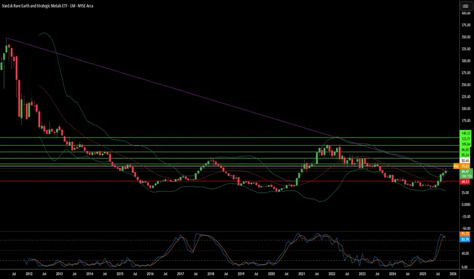
For investors, the VanEck Rare Earth/Strategic Metals ETF (REMX) operates as a direct proxy for geopolitical risk rather than traditional commodity exposure. Neodymium oxide prices, which plummeted from $209.30 per kilogram in January 2023 to $113.20 in January 2024, are projected to surge to $150.10 by October 2025 volatility driven not by physical scarcity but by regulatory announcements and supply chain weaponization. The investment thesis hinges on three pillars: China's processing monopoly converted into political leverage, exponential green technology demand establishing a robust price floor, and Western industrial policy guaranteeing long-term financing for diversification. Success will favor companies establishing verifiable, resilient supply chains in downstream processing and magnet manufacturing outside China, though the high costs of secure supply, including mandatory cybersecurity auditing and environmental compliance, ensure elevated prices for the foreseeable future.
Risk On/Off: How Global Correlations Tell You Money Flow🔵 Risk On / Risk Off: How Global Correlations Tell You Where Money Is Flowing
Difficulty: 🐳🐳🐳🐋🐋 (Intermediate+)
This article is for traders who want to understand how global capital flow affects market behavior — from equities and crypto to gold and bonds. Learning to read “Risk On” and “Risk Off” regimes helps you anticipate big shifts before they hit your chart.
🔵 INTRODUCTION
Markets are not independent islands — they are connected by one universal force: liquidity flow .
When investors feel confident, they move capital into riskier assets like stocks and crypto — this is called Risk On .
When fear dominates, capital flows back into safety — bonds, gold, and the U.S. dollar — known as Risk Off .
Recognizing this rotation allows traders to align their bias with the flow of global capital rather than fighting it.
🔵 WHAT IS “RISK ON”
Risk On is a market environment where investors seek higher returns, volatility is subdued, and capital flows into assets with greater reward potential.
Typical Risk-On behavior:
S&P 500, Nasdaq, and other equities trend higher
Bitcoin and crypto assets outperform traditional markets
U.S. Dollar Index (DXY) weakens as money moves abroad
Bond yields rise moderately as investors leave safe assets
Gold often consolidates or declines
In simple terms: Money chases opportunity.
🔵 WHAT IS “RISK OFF”
Risk Off describes defensive conditions — fear rises, volatility expands, and liquidity seeks safety.
Typical Risk-Off behavior:
S&P 500 and risk assets decline
Bitcoin and altcoins drop sharply
DXY strengthens as investors move into USD
Bond yields fall as money enters treasuries
Gold rallies as a safe-haven hedge
In simple terms: Money runs to safety.
🔵 HOW TO DETECT RISK SHIFTS
Market regimes don’t flip instantly — they rotate through correlated behavior.
To identify the shift between Risk On and Risk Off, monitor key macro instruments together:
DXY (Dollar Index): Rising DXY = Risk Off sentiment, Falling DXY = Risk On.
SPX / NASDAQ: Strong uptrends = Risk On, persistent weakness = Risk Off.
BTC vs DXY: Inverse correlation; BTC strength with DXY weakness = liquidity expansion.
Bond Yields (US10Y): Rising = optimism, Falling = risk aversion.
VIX Index: Below 15 = complacent Risk On, Above 25 = fearful Risk Off.
🔵 THE GLOBAL LIQUIDITY CYCLE
Liquidity always moves in phases — expansion, acceleration, contraction, and reset.
Phase 1 – Liquidity Expansion: Central banks inject liquidity → Risk On begins.
Phase 2 – Overextension: Assets rally strongly, leverage increases, volatility stays low.
Phase 3 – Liquidity Contraction: Monetary tightening or policy shocks trigger Risk Off.
Phase 4 – Repricing & Reset: Markets bottom as new liquidity returns.
Understanding this rhythm helps traders avoid confusion when markets seem “irrational” — because they’re not, they’re simply rotating through the liquidity cycle.
🔵 USING RISK ON/OFF IN TRADING
Even technical traders benefit from recognizing global risk regimes.
By aligning with the dominant liquidity direction, setups gain higher probability.
Crypto traders: Use SPX, DXY, and VIX correlations to confirm momentum.
Stock traders: Track gold and yields to gauge investor confidence.
Forex traders: Trade USD pairs according to global sentiment.
Swing traders: Filter trade bias by checking the current global regime.
Tip: When correlations align (e.g., DXY up, SPX down, BTC down), expect trend continuation.
When they diverge, volatility or reversals are likely.
🔵 ADVANCED TOOLS TO WATCH
Global Liquidity Index: Track combined balance sheets of the Fed, ECB, BOJ, and PBC.
Stablecoin Supply (Crypto): Expanding supply = liquidity entering market.
Yield Curve (10Y–2Y spread): Falling = caution, Rising = recovery.
Funding Rates: Confirm risk sentiment via leverage buildup.
🔵 CONCLUSION
All markets are connected through liquidity.
Risk On and Risk Off regimes describe how that liquidity rotates between return and safety. By tracking global correlations — equities, bonds, gold, DXY, and crypto — traders gain a powerful macro filter to stay on the right side of momentum.
Liquidity creates direction. Correlation confirms conviction.
If you learn to read the global flow, your technical analysis will finally make sense in the bigger picture.
Do you track global correlations in your analysis? What’s your favorite Risk-On or Risk-Off indicator?
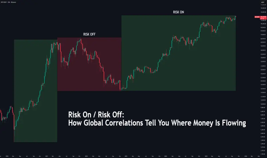
Why Most Traders Blow Their Accounts?
It’s not bad strategy; it’s bad risk.
Most traders break before their accounts do. They revenge trade, double down, or skip stops because they can’t stand being wrong.
Here’s the truth: Discipline beats setups every time in my perspective.
Try this today →
Risk 0.5% per trade for one week.
If you can’t follow that rule, it’s not the market that’s broken; it’s your system of control.
I’ve been testing something that helps traders stay inside their limits when emotions spike.
Want me to share how it works?
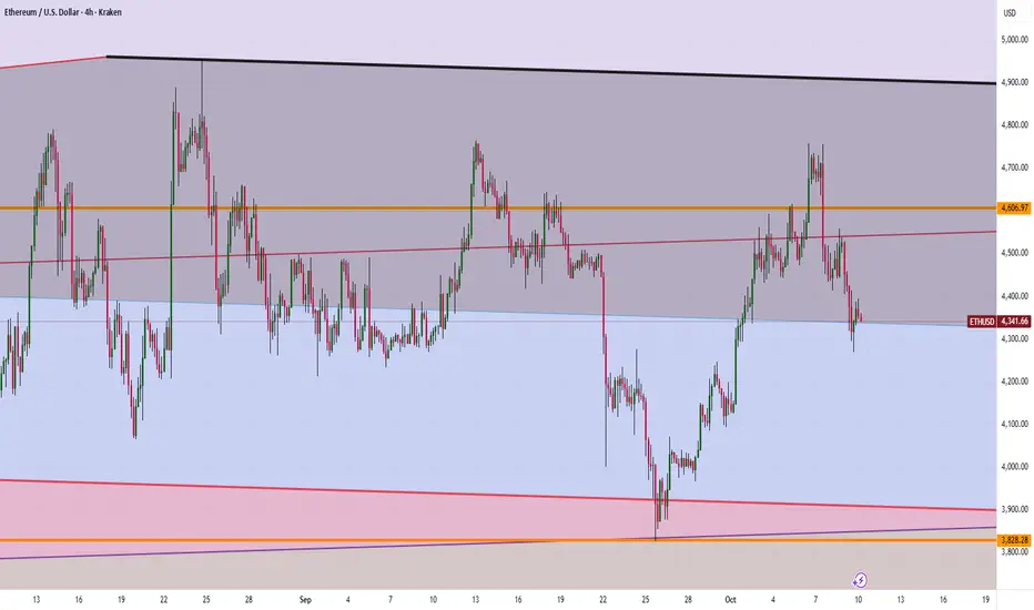
Trading Psychology Bias Lesson: BTCUSD 1D ATR Position SizeSummary
Bias shifts judgment under stress and often decides outcomes before the order ticket. This idea converts trading psychology into rules you can apply on BTCUSD now. It uses fixed ATR stops, pre defined entries and exits, a written disconfirming note before any order, and decision grades based on rule adherence. The goal is tighter drawdowns and consistent execution across regimes.
Live context
Price 123,102
SMA 50 114,314
EMA 200 106,289
ATR 14 daily 2,882.52 which is 2.34% of price
Distance to SMA 50 is 8,788 which is 7.14%
Distance to EMA 200 is 16,813 which is 13.66%
2 x ATR equals 5,765.04 which is 4.68%
Why psychology decides the trade before entry
Real trading includes noise, limited attention, and emotion. The result is bias, a stable tendency that pulls choices away from the written rule. Bias creeps into 4 moments: setup definition, entry trigger, position size, exit and review. The fix is structure. Use 5 blocks: a 1 sentence setup, entry and stop and trail defined with ATR, a written disconfirming note, a higher timeframe check, and a post trade grade by rule adherence rather than outcome.
Theory. Core biases you must neutralize
Loss aversion . Loss pain exceeds gain pleasure and leads to widening stops or cutting winners early. Fix . Initial stop equals 2 x ATR. Trail equals 1 x ATR or a close through a moving reference. Never widen stops.
Confirmation bias . You search for evidence that agrees with your idea. Fix . Write 1 disconfirming fact before any order. Check the next higher timeframe. If it disagrees, cut size by 50% or skip.
Anchoring . You fixate on entry or a round level. Fix . Define exits on structure with ATR or a moving average close. Name the anchor in notes to reduce its pull.
Recency and availability . You overweight the last 1 to 3 candles. Fix . Use a 20 bar context rule and a weekly system review.
Overconfidence . After a win trade count and size increase without any change in edge. Fix . Cool down 2 minutes after every exit and halve next size after a large winner.
Herd and gambler’s fallacy . Late entries on wide candles and belief that streaks must continue or must reverse. Fix . Only take trades with projected reward to risk at least 2 to 1 at the planned stop and avoid high impact events.
Hindsight and outcome bias . You judge by result and rewrite rules after 1 loss. Fix . Save entry and exit screenshots and grade by rule adherence.
Status quo and endowment . You sit in positions you already own while better setups exist. Fix . Monthly retest of every holding against current rules.
Three guardrail rules for BTCUSD
Stop discipline. Initial stop equals 2 x ATR. Trail winners by 1 x ATR or by a daily close through SMA 50. Do not widen stops.
Decision hygiene. Before every order write 1 disconfirming fact and check the next higher timeframe. If the higher timeframe disagrees, cut size by 50% or skip.
Quality floor. Projected reward to risk is at least 2 to 1 at the initial stop distance.
BTCUSD 1D continuation plan with exact math
This plan assumes a breakout continuation and uses your live ATR 14. All digits are based on ATR 2,882.52 and a price above SMA 50 and EMA 200.
Setup in 1 sentence . Trend continuation long on a daily close above the recent swing with SMA 50 rising and 20 bar context bullish.
Entry trigger . Close above 124,200 confirms continuation.
Initial risk . 2 x ATR equals 5,765.04. Stop equals entry minus 5,765.04. For 124,200 the stop is 118,434.96.
Targets . 1R target equals entry plus 5,765.04 which is 129,965.04. 2R target equals entry plus 11,530.08 which is 135,730.08.
Sizing example . Equity 20,000. Risk per trade 1% equals 200. Position size equals risk divided by stop distance which is 200 ÷ 5,765.04 equals 0.0347 BTC. Notional at 124,200 is about 4,308.
Management . Trail by 1 x ATR which is 2,882.52. Move the stop only with the trail. Ignore the first single red candle to reduce recency effects.
Exit logic . Exit on a daily close below the 1 x ATR trail or use a time stop after 12 bars if 2R is not reached.
Journal cue . Before entry write 1 disconfirming fact. After exit save 2 screenshots and grade by rule adherence.
Why each step neutralizes bias in real time
Loss aversion is capped because the stop distance is fixed by ATR and never widened. The trail is mechanical.
Confirmation is checked by the written disconfirming fact and the higher timeframe review that can force a skip or a 50% position cut.
Anchoring is reduced because exits reference ATR and structure instead of entry or round numbers.
Recency is filtered by the 20 bar rule and by a weekly system review that ignores single outcomes.
Overconfidence is constrained by a 2 minute cool down and 50% next size after a large winner.
Mean reversion companion inside an uptrend
Use this only while SMA 50 and EMA 200 slope up and price trades above both averages.
Context . Pullback forms inside the 20 bar range toward short term support while SMA 50 rises above EMA 200.
Entry . Bullish rejection from a prior swing zone or a daily close back above the intraday pivot after a 2 to 3 day pause.
Risk . Initial stop equals 1.5 x ATR which is 4,323.78.
Sizing . Risk per trade 1%. Position size equals risk divided by 4,323.78. With equity 20,000 and risk 200 the size equals 0.0463 BTC.
Exit . First scale at 1.5 R. Stop to break even only after a daily close above SMA 50. Final exit at 2 R or on a daily close back into the pullback range.
Bias note . Write 1 anchor you feel and 1 disconfirming fact that would cancel the setup.
Decision checklist to paste into chart notes
Setup in 1 sentence written before entry
Entry level, initial stop, trail method defined
1 disconfirming fact written and verified
Higher timeframe checked and size adjusted if needed
Projected reward to risk is at least 2 to 1
Screenshots saved at entry and exit
Decision grade recorded by rule adherence
Position size rule you can audit weekly
Account equity E. Risk per trade equals 1% of E by default.
Stop distance equals the ATR multiple from the plan.
Position size equals risk divided by stop distance. If required size is not tradable, skip the trade.
Bias symptoms you will see on the BTCUSD chart and the fix
Loss aversion . Stops drift lower while price falls. Winners are cut early. Fix . 2 x ATR hard stop and 1 x ATR trail.
Confirmation . Indicators are added until they agree with your view. Fix . 1 written disconfirming note and a higher timeframe check.
Anchoring . Waiting to exit when price returns to entry or to a round level. Fix . Structure based exits and naming the anchor in notes.
Recency . Judgment based on the last 2 candles. Fix . 20 bar context rule and a weekly system review.
Overconfidence . Trade count jumps after a win. Fix . 2 minute cool down and 50% next size after a large winner.
Herd and gambler’s fallacy . Late entries on wide candles and streak thinking. Fix . 2 to 1 minimum reward to risk and a news ban during known high impact windows.
Hindsight and outcome bias . Rewriting rules after 1 result. Fix . Grade by rule adherence and keep entry plus exit screenshots.
Status quo and endowment . Sitting in flat positions you already own. Fix . Monthly retest of every holding against current rules.
Worked example with our numbers
Assuming a daily close above 124,200 triggers the continuation. Initial stop equals 2 x ATR which is 5,765.04. Stop equals 118,434.96. 1R target equals 129,965.04. 2R target equals 135,730.08. Equity equals 20,000. Risk equals 200. Position size equals 0.0347 BTC. As price advances you trail by 1 x ATR which is 2,882.52 and you move the stop only when the trail shifts. If the trail is hit you exit. If 12 bars pass without the 2R target you exit on time and log the decision. You do not widen the stop. You do not add size after a win. You grade the decision by rule adherence.
If momentum stalls
If a daily close rotates down toward 121,000 to 121,500 and momentum weakens, shift to neutral. Wait for a fresh setup that passes the 2 to 1 test at the planned stop.
Do not react to a single candle. The plan lives on the daily chart.
Comparator and scorecard
Use simple Buy and Hold on BTCUSD as the baseline. Score the plan by Return divided by Drawdown, Max Drawdown, and percent of trades executed exactly as written. A smaller drawdown with steady execution beats a higher raw return with poor adherence. Your best forward indicator is the discipline metric you log each week.
Education and analytics only. Not investment advice. Test any rule with historical data before risking capital.

BTC Tests Range Highs Below 120k: Wait for Confirmation __________________________________________________________________________________
Market Overview
__________________________________________________________________________________
BTC is back at the top of its range, pressing 116.8k–117.97k just beneath the 120k barrier. Higher timeframes (12H/1D) lean bullish, while mid-TFs still push back — confirmation is key before chasing strength.
Momentum: 📈 Cautiously bullish; above 115.2k, a clean close >117.97k would likely unlock 120k.
Key levels: Resistances: 116.8k–117.97k; 120k; 124.3k. Supports: 115.2k; 114k; 112.4k–111.1k.
Volumes: Very high on 6H→30m (mostly under resistance), normal on 1D.
Multi-timeframe signals: 1D/12H Up; 6H/4H/2H Down; 1H/30m/15m Up.
Risk On / Risk Off Indicator context: NEUTRE VENTE — slight risk-off, contradicting daily momentum.
__________________________________________________________________________________
Trading Playbook
__________________________________________________________________________________
With range highs overhead, stay constructive but disciplined: lean cautiously bullish while 115.2k holds and wait for confirmed breaks to avoid traps.
Global bias: Cautious bullish while 115.2k holds; major invalidation on a 1D close <114k.
Opportunities:
• Pullback buy if 115.2k holds, then confirm >116.8k.
• Breakout long on 1D close >117.97k; add if 120k flips to support.
• Tactical sell on rejection at 116.8k–117.97k toward 115.2k then 114k.
Risk zones / invalidations: Loss of 115.2k opens 114k/112.4k; a 1D close >120.6k invalidates top-shorts.
Macro catalysts: Fed −25 bps (supports risk), potential US data timing shifts (ISM/NFP) that can cluster volatility, and positive BTC spot ETF flows (Day +$430M) reinforcing dips.
Action plan: Entry >117.97k (≥2 closes + retest) / Stop <115.8k / TP1 120k, TP2 122.5k, TP3 124.3k / R:R ~1.8–2.5.
__________________________________________________________________________________
Multi-Timeframe Insights
__________________________________________________________________________________
Higher timeframes point up, but mid-TF supply still caps price near the range highs; intraday strength needs follow-through to avoid bull traps.
1D/12H: Holding above 115.2k preserves upside bias; convert 117.97k to open 120k then 124.3k.
6H/4H/2H: Seller pressure below 116.8k–117.5k; beware fake breaks without volume follow-through.
1H/30m/15m: Impulsive bounce is constructive, but requires break/hold (≥2 bars) to confirm trend continuation.
__________________________________________________________________________________
Macro & On-Chain Drivers
__________________________________________________________________________________
A supportive macro backdrop and improving flows help, but timing risks keep volatility elevated around resistance.
Macro events: Fed easing (−25 bps) underpins risk appetite; shifting ISM/NFP timing may concentrate moves around data windows.
Bitcoin analysis: 114k–115.2k defended; highest quarterly close; weekly ETF inflows turned positive.
On-chain data: STH cost basis ~111k; ETF inflows resumed; recent deleveraging cleans positioning.
Expected impact: Slight bullish tilt if 115.2k holds and 117.97k flips to support; otherwise risk of 114k/112.4k retests.
__________________________________________________________________________________
Key Takeaways
__________________________________________________________________________________
BTC is pressing range highs with active supply below 120k. The cleaner long is a confirmed breakout >117.97k with 120k turning into support; otherwise, fading rejections back into 115.2k remains valid. Macro support (−25 bps + positive ETF flows) helps, but confirmation at resistance matters most. Stay patient and execute only on validated signals.
