PRO Investing - Apex EnginePRO Investing - Apex Engine
1. Core Concept: Why Does This Indicator Exist?
Traditional momentum oscillators like RSI or Stochastic use a fixed "lookback period" (e.g., 14). This creates a fundamental problem: a 14-period setting that works well in a fast, trending market will generate constant false signals in a slow, choppy market, and vice-versa. The market's character is dynamic, but most tools are static.
The Apex Engine was built to solve this problem. Its primary innovation is a self-optimizing core that continuously adapts to changing market conditions. Instead of relying on one fixed setting, it actively tests three different momentum profiles (Fast, Mid, and Slow) in real-time and selects the one that is most synchronized with the current price action.
This is not just a random combination of indicators; it's a deliberate synthesis designed to create a more robust momentum tool. It combines:
Volatility analysis (ATR) to generate adaptive lookback periods.
Momentum measurement (ROC) to gauge the speed of price changes.
Statistical analysis (Correlation) to validate which momentum measurement is most effective right now.
Classic trend filters (Moving Average, ADX) to ensure signals are only taken in favorable market conditions.
The result is an oscillator that aims to be more responsive in volatile trends and more stable in quiet periods, providing a more intelligent and adaptive signal.
2. How It Works: The Engine's Three-Stage Process
To be transparent, it's important to understand the step-by-step logic the indicator follows on every bar. It's a process of Adapt -> Validate -> Signal.
Stage 1: Adapt (Dynamic Length Calculation)
The engine first measures market volatility using the Average True Range (ATR) relative to its own long-term average. This creates a volatility_factor. In high-volatility environments, this factor causes the base calculation lengths to shorten. In low-volatility, they lengthen. This produces three potential Rate of Change (ROC) lengths: dynamic_fast_len, dynamic_mid_len, and dynamic_slow_len.
Stage 2: Validate (Self-Optimizing Mode Selection)
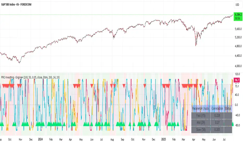
This is the core of the engine. It calculates the ROC for all three dynamic lengths. To determine which is best, it uses the ta.correlation() function to measure how well each ROC's movement has correlated with the actual bar-to-bar price changes over the "Optimization Lookback" period. The ROC length with the highest correlation score is chosen as the most effective profile for the current moment. This "active" mode is reflected in the oscillator's color and the dashboard.
Stage 3: Signal (Normalized Velocity Oscillator)
The winning ROC series is then normalized into a consistent oscillator (the Velocity line) that ranges from -100 (extreme oversold) to +100 (extreme overbought). This ensures signals are comparable across any asset or timeframe. Signals are only generated when this Velocity line crosses its signal line and the trend filters (explained below) give a green light.
3. How to Use the Indicator: A Practical Guide
Reading the Visuals:
Velocity Line (Blue/Yellow/Pink): The main oscillator line. Its color indicates which mode is active (Fast, Mid, or Slow).
Signal Line (White): A moving average of the Velocity line. Crossovers generate potential signals.
Buy/Sell Triangles (▲ / ▼): These are your primary entry signals. They are intentionally strict and only appear when momentum, trend, and price action align.
Background Color (Green/Red/Gray): This is your trend context.
Green: Bullish trend confirmed (e.g., price above a rising 200 EMA and ADX > 20). Only Buy signals (▲) can appear.
Red: Bearish trend confirmed. Only Sell signals (▼) can appear.
Gray: No clear trend. The market is likely choppy or consolidating. No signals will appear; it is best to stay out.
Trading Strategy Example:
Wait for a colored background. A green or red background indicates the market is in a tradable trend.
Look for a signal. For a green background, wait for a lime Buy triangle (▲) to appear.
Confirm the trade. Before entering, confirm the signal aligns with your own analysis (e.g., support/resistance levels, chart patterns).
Manage the trade. Set a stop-loss according to your risk management rules. An exit can be considered on a fixed target, a trailing stop, or when an opposing signal appears.
4. Settings and Customization
This script is open-source, and its settings are transparent. You are encouraged to understand them.
Synaptic Engine Group:
Volatility Period: The master control for the adaptive engine. Higher values are slower and more stable.
Optimization Lookback: How many bars to use for the correlation check.
Switch Sensitivity: A buffer to prevent frantic switching between modes.
Advanced Configuration & Filters Group:
Price Source: The data source for momentum calculation (default close).
Trend Filter MA Type & Length: Define your long-term trend.
Filter by MA Slope: A key feature. If ON, allows for "buy the dip" entries below a rising MA. If OFF, it's stricter, requiring price to be above the MA.
ADX Length & Threshold: Filters out non-trending, choppy markets. Signals will not fire if the ADX is below this threshold.
5. Important Disclaimer
This indicator is a decision-support tool for discretionary traders, not an automated trading system or financial advice. Past performance is not indicative of future results. All trading involves substantial risk. You should always use proper risk management, including setting stop-losses, and never risk more than you are prepared to lose. The signals generated by this script should be used as one component of a broader trading plan.
Correlation
Asset Premium/Discount Monitor📊 Overview
The Asset Premium/Discount Monitor is a tool for analyzing the relative value between two correlated assets. It measures when one asset is trading at a premium or discount compared to its historical relationship with another asset, helping traders identify potential mean reversion opportunities, or pairs trading opportunities.
🎯 Use Cases
Perfect for analyzing:
NASDAQ:MSTR vs CRYPTO:BTCUSD - MicroStrategy's premium/discount to Bitcoin
NASDAQ:COIN vs BITSTAMP:BTCUSD - Coinbase's relative value to Bitcoin
NASDAQ:TSLA vs NASDAQ:QQQ - Tesla's premium to tech sector
Regional banks AMEX:KRE vs AMEX:XLF - Individual bank stocks vs financial sector
Any two correlated assets where relative value matters
Example of a trade: MSTR vs BTC - When indicator shows MSTR at 95% percentile (extreme premium): Short MSTR, Buy BTC. Then exit when the spread reverts to the mean, say 40-60% percentile.
🔧 How It Works
Core Calculation
Ratio Analysis: Calculates the price ratio between your asset and the correlated asset
Historical Baseline: Establishes the "normal" relationship using a 252-day moving average. You can change this.
Premium Measurement: Measures current deviation from historical average as a percentage
Statistical Context: Provides percentile rankings and standard deviation bands
The Math
Premium % = (Current Ratio / Historical Average Ratio - 1) × 100
🎨 Customization Options
Correlated Asset: Choose any symbol for comparison
Lookback Period: Adjust historical baseline (50-1000 days)
Smoothing: Reduce noise with moving average (1-50 days)
Visual Toggles: Show/hide bands and percentile lines
Color Themes: Customize premium/discount colors
📊 Interpretation Guide
Premium/Discount Reading
Positive %: Asset trading above historical relationship (premium)
Negative %: Asset trading below historical relationship (discount)
Near 0%: Asset at fair value relative to correlation
Percentile Ranking
90%+: Near recent highs - potential selling opportunity
10% and below: Near recent lows - potential buying opportunity
25-75%: Normal trading range
Signal Classifications
🔴 SELL PREMIUM: Asset expensive relative to recent range
🟡 Premium Rich: Moderately expensive, monitor for reversal
⚪ NEUTRAL: Fair value territory
🟡 Discount Opportunity: Moderately cheap, potential accumulation zone
🟢 BUY DISCOUNT: Asset cheap relative to recent range
🚨 Built-in Alerts
Extreme Premium Alert: Triggers when percentile > 95%
Extreme Discount Alert: Triggers when percentile < 5%
⚠️ Important Notes
Works best with highly correlated assets
Historical relationships can change - monitor correlation strength
Not investment advice - use as one factor in your analysis
Backtest thoroughly before implementing any strategy
🔄 Updates & Future Features
This indicator will be continuously improved based on user feedback. So... please give me your feedback!

Intermarket Correlation Oscillator (ICO)The Intermarket Correlation Oscillator (ICO) is a TradingView indicator that helps traders analyze the relationship between two assets, such as stocks, indices, or cryptocurrencies, by measuring their price correlation. It displays this correlation as an oscillator ranging from -1 to +1, making it easy to spot whether the assets move together, oppositely, or independently. A value near +1 indicates strong positive correlation (assets move in the same direction), near -1 shows strong negative correlation (opposite movements), and near 0 suggests no correlation. This tool is ideal for confirming trends, spotting divergences, or identifying hedging opportunities across markets.
How It Works?
The ICO calculates the Pearson correlation coefficient between the chart’s primary asset (e.g., Apple stock) and a secondary asset you choose (e.g., SPY for the S&P 500) over a specified number of bars (default: 20). The oscillator is plotted in a separate pane below the chart, with key levels at +0.8 (overbought, strong positive correlation) and -0.8 (oversold, strong negative correlation). A midline at 0 helps gauge neutral correlation. When the oscillator crosses these levels or the midline, labels ("OB" for overbought, "OS" for oversold) and alerts notify you of significant shifts. Shaded zones highlight extreme correlations (red for overbought, green for oversold) if enabled.
Why Use the ICO?
Trend Confirmation: High positive correlation (e.g., SPY and QQQ both rising) confirms market trends.
Divergence Detection: Negative correlation (e.g., DXY rising while stocks fall) signals potential reversals.
Hedging: Identify negatively correlated assets to balance your portfolio.
Market Insights: Understand how assets like stocks, bonds, or crypto interact.
Easy Steps to Use the ICO in TradingView
Add the Indicator:
Open TradingView and load your chart (e.g., AAPL on a daily timeframe).
Go to the Pine Editor at the bottom of the TradingView window.
Copy and paste the ICO script provided earlier.
Click "Add to Chart" to display the oscillator below your price chart.
Configure Settings:
Click the gear icon next to the indicator’s name in the chart pane to open settings.
Secondary Symbol: Choose an asset to compare with your chart’s symbol (e.g., "SPY" for S&P 500, "DXY" for USD Index, or "BTCUSD" for Bitcoin). Default is SPY.
Correlation Lookback Period: Set the number of bars for calculation (default: 20). Use 10-14 for short-term trading or 50 for longer-term analysis.
Overbought/Oversold Levels: Adjust thresholds (default: +0.8 for overbought, -0.8 for oversold) to suit your strategy. Lower values (e.g., ±0.7) give more signals.
Show Midline/Zones: Check boxes to display the zero line and shaded overbought/oversold zones for visual clarity.
Interpret the Oscillator:
Above +0.8: Strong positive correlation (red zone). Assets move together.
Below -0.8: Strong negative correlation (green zone). Assets move oppositely.
Near 0: No clear relationship (midline reference).
Labels: "OB" or "OS" appears when crossing overbought/oversold levels, signaling potential correlation shifts.
Set Up Alerts:
Right-click the indicator, select "Add Alert."
Choose conditions like "Overbought Alert" (crossing above +0.8), "Oversold Alert" (crossing below -0.8), or zero-line crossings for bullish/bearish correlation shifts.
Configure notifications (e.g., email, SMS) to stay informed.
Apply to Trading:
Use positive correlation to confirm trades (e.g., buy AAPL if SPY is rising and correlation is high).
Spot divergences for reversals (e.g., stocks dropping while DXY rises with negative correlation).
Combine with other indicators like RSI or moving averages for stronger signals.
Tips for New Users
Start with related assets (e.g., SPY and QQQ for tech stocks) to see clear correlations.
Test on a demo account to understand signals before trading live.
Be aware that correlation is a lagging indicator; confirm signals with price action.
If the secondary symbol doesn’t load, ensure it’s valid on TradingView (e.g., use correct ticker format).
The ICO is a powerful, beginner-friendly tool to explore intermarket relationships, enhancing your trading decisions with clear visual cues and alerts.

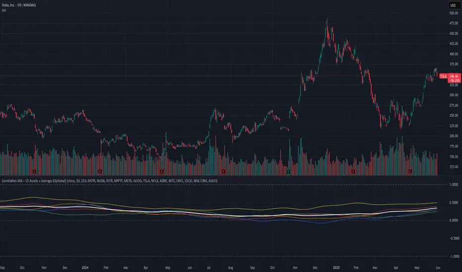
Correlation MA – 15 Assets + Average (Optional)This indicator calculates the moving average of the correlation coefficient between your charted asset and up to 15 user-selected symbols. It helps identify uncorrelated or inversely correlated assets for diversification, pair trading, or hedging.
Features:
✅ Compare your current chart against up to 15 assets
✅ Toggle assets on/off individually
✅ Custom correlation and MA lengths
✅ Real-time average correlation line across enabled assets
✅ Horizontal lines at +1, 0, and -1 for easy visual reference
Ideal for:
Portfolio diversification analysis
Finding low-correlation stocks
Mean-reversion & pair trading setups
Crypto, equities, ETFs
To use: set the benchmark chart (e.g. TSLA), choose up to 15 assets, and adjust settings as needed. Look for assets with correlation near 0 or negative values for uncorrelated performance.
Correlation Coefficient📊 Correlation Coefficient (CC)
This indicator measures the statistical correlation between two selected securities over a defined period, scaled from -100 to +100.
It helps you quickly assess whether assets are moving:
Together (positive correlation)
Opposite (negative correlation)
Independently (zero correlation)
🔧 Features:
Select any two symbols (default: NIFTY & BANKNIFTY)
Adjustable length parameter for short-term or long-term correlation analysis
Clean, color-coded plot with horizontal levels to easily identify key correlation zones
📈 Useful For:
Pair trading setups
Hedging strategies
Detecting market regime shifts or intermarket divergences
⚠️ Disclaimer: This is not trading or investment advice.
This indicator is intended for informational purposes only and is not recommended for making
direct trading decisions.

Statistical Pairs Trading IndicatorZ-Score Stat Trading — Statistical Pairs Trading Indicator
📊🔗
---
What is it?
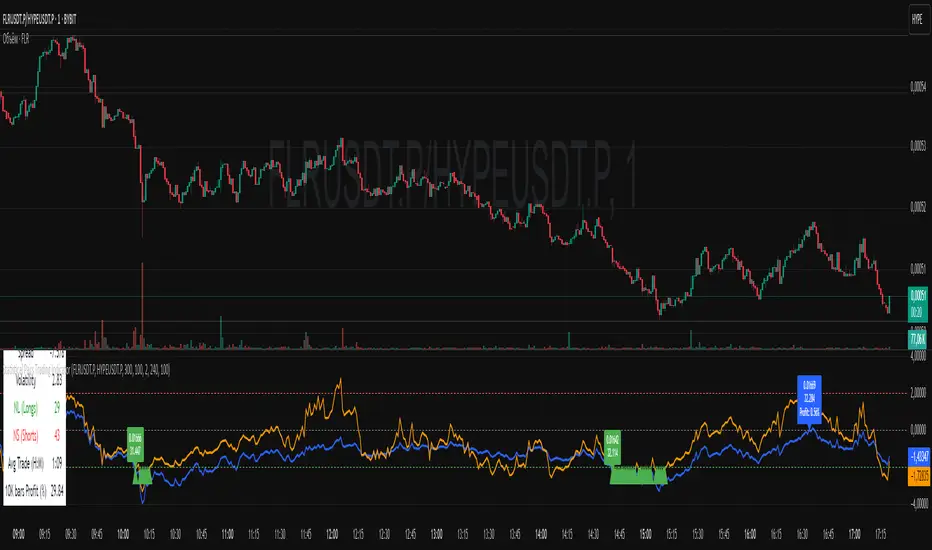
Z-Score Stat Trading is a powerful indicator for statistical pairs trading and quantitative analysis of two correlated assets.
It calculates the Z-Score of the log-price spread between any two symbols you choose, providing both long-term and short-term Z-Score signals.
You’ll also see real-time correlation, volatility, spread, and the number of long/short signals in a handy on-chart table!
---
How to Use 🛠️
1. Add the indicator to your chart.
2. Select two assets (symbols) to analyze in the settings.
3. Watch the Z-Score plots (blue and orange lines) and threshold levels (+2, -2 by default).
4. Check the info table for:
- Correlation
- Volatility
- Spread
- Number of long (NL) and short (NS) signals in the last 1000 bars
5. Set up alerts for signal generation or threshold crossings if you want to be notified automatically.
---
Trading Strategy 💡
- This indicator is designed for statistical arbitrage (mean reversion) strategies.
- Long Signal (🟢):
When both Z-Scores drop below the negative threshold (e.g., -2), a long signal is generated.
→ Buy Symbol A, Sell Symbol B, expecting the spread to revert to the mean.
- Short Signal (🔴):
When both Z-Scores rise above the positive threshold (e.g., +2), a short signal is generated.
→ Sell Symbol A, Buy Symbol B, again expecting mean reversion.
- The info table helps you quickly assess the frequency of signals and the current statistical relationship between your chosen assets.
---
Best Practices & Warnings 🚦
- Avoid high leverage! Pairs trading can be risky, especially during periods of divergence. Use conservative position sizing.
- Check for cointegration: Before using this indicator, make sure both assets are cointegrated or have a strong historical relationship. This increases the reliability of mean reversion signals.
- Check correlation: Only use asset pairs with a high correlation (preferably 0.8–0.9 or higher) for best results. The correlation value is shown in the info table.
- Scale in and out gradually: When entering or exiting positions, consider doing so in parts rather than all at once. This helps manage slippage and risk, especially in volatile markets.
---
⚠️ Note on Performance:
This indicator may work a bit slowly, especially on large timeframes or long chart histories, because the calculation of NL and NS (number of long/short signals) is computationally intensive.
---
Disclaimer ⚠️
This script is provided for educational and informational purposes only .
It is not financial advice or a recommendation to buy or sell any asset.
Use at your own risk. The author assumes no responsibility for any trading decisions or losses.
CorrelationMulti-Timeframe Correlation Indicator
This Pine Script indicator measures the correlation between the current symbol and a reference symbol (default: GLD) across three different timeframes. It provides traders with valuable insights into how assets move in relation to each other over short, medium, and long-term periods.
Key Features
Multiple Timeframe Analysis: Calculates correlation coefficients over three customizable periods (default: 20, 50, and 200 bars)
Visual Reference Lines: Displays horizontal lines at +1, 0, and -1 to indicate perfect positive correlation, no correlation, and perfect negative correlation
Color-Coded Outputs: Shows short-term correlation in green, medium-term in yellow, and long-term in red for easy visual interpretation
Understanding Correlation
The correlation coefficient measures the statistical relationship between two data series, ranging from -1 to +1:
+1: Perfect positive correlation (both assets move together in the same direction)
0: No correlation (movements are random and independent)
-1: Perfect negative correlation (assets move in opposite directions)
How To Use This Indicator
Market Relationships: Identify how strongly your current asset correlates with the reference symbol
Diversification Analysis: Find assets with negative correlations to build a diversified portfolio
Divergence Opportunities: Watch for changes in correlation patterns that might signal trading opportunities
Trend Confirmation: Use correlation with benchmark assets to confirm broader market trends
Customization Options
Reference Symbol: Change the default GLD to any other symbol you want to compare against
Period Lengths: Adjust the short, medium, and long timeframes to match your trading strategy and timeframe
This indicator helps traders make more informed decisions by understanding the interrelationships between different assets across various timeframes, potentially improving portfolio construction and risk management strategies.

SMT Divergence ICT 02 [TradingFinder] Smart Money Technique SMC🔵 Introduction
SMT Divergence (Smart Money Technique Divergence) is a price action-based trading concept that detects discrepancies in market behavior between two assets that are generally expected to move in the same direction. Rooted in ICT (Inner Circle Trader) methodology, this approach helps traders recognize subtle signs of market manipulation or imbalance, often ahead of traditional indicators.
The core idea behind SMT divergence is simple: when two correlated instruments—such as currency pairs, indices, or assets from the same sector—start forming different swing points (highs or lows), this can reveal a lack of confirmation in the trend. Such divergence is often a precursor to a price reversal or pause in momentum.
This technique works effectively across various markets including Forex, stocks, and cryptocurrencies. It’s particularly valuable when used alongside concepts like liquidity sweeps, market structure breaks (MSBs), or order block identification.
In advanced use cases, Sequential SMT helps uncover patterns of alternating divergences across sessions, often signaling engineered liquidity traps before price reacts.
When combined with the Quarterly Theory—which segments market behavior into Accumulation, Manipulation, Distribution, and Continuation/Reversal phases—traders gain insight not only into where divergence happens, but when it's most likely to be significant within the market cycle.
Bullish SMT :
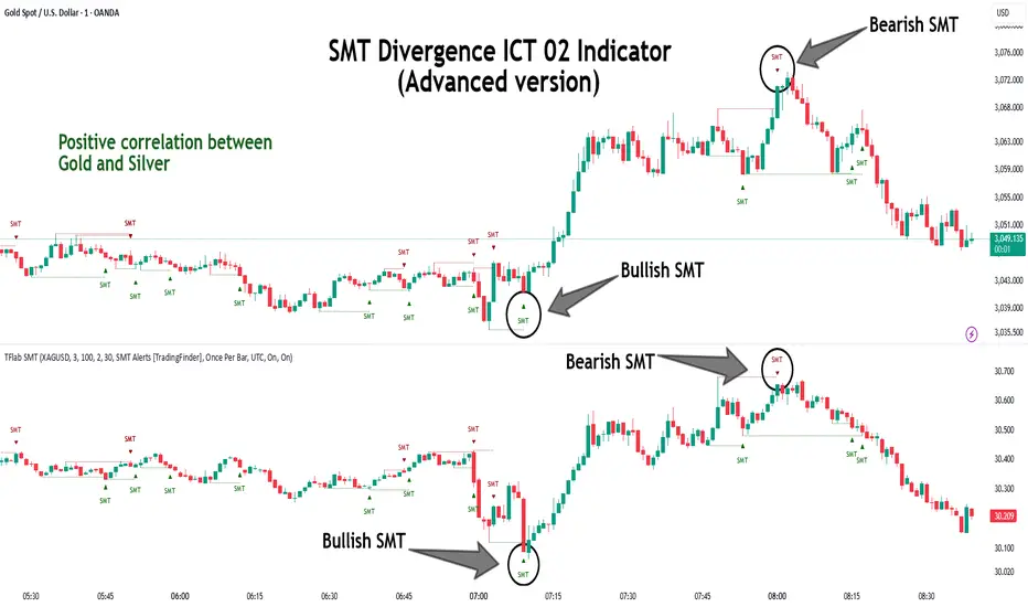
Bullish SMT Divergence occurs when one asset prints a higher low while the correlated asset forms a lower low. This asymmetry often suggests that the downside move is losing strength, hinting at a potential bullish shift.
Bearish SMT :
Bearish SMT Divergence is formed when one asset creates a higher high, while the second asset fails to confirm by printing a lower high. This typically signals weakening bullish pressure and the possibility of a reversal to the downside.
🔵 How to Use
The SMT Divergence indicator is designed to detect imbalances between two positively correlated assets—such as major currency pairs, indices, or commodities. These divergences often indicate early signs of market inefficiency or smart money manipulation and can help traders anticipate trend shifts with higher precision.
Unlike traditional divergence indicators or earlier versions of this script, this upgraded version does not rely solely on consecutive pivot comparisons. Instead, it dynamically scans all available pivots within the chart to identify divergences at any structural level—major or minor—across the price action. This broader detection method increases the reliability and frequency of meaningful SMT signals.
Moreover, when integrated with Sequential SMT logic, the indicator is capable of identifying multiple divergence sequences across sessions. These sequences often signal engineered liquidity traps and can be mapped within the Quarterly Theory framework, allowing traders to pinpoint not just the presence of divergence but also the phase of the market cycle it appears in (Accumulation, Manipulation, Distribution, or Continuation).
🟣 Bullish SMT Divergence
This signal occurs when the primary asset forms a higher low, while the correlated asset forms a lower low. This pattern implies weakening bearish momentum and a potential shift to the upside.
If the correlated asset breaks its previous low but the primary asset does not, this divergence suggests absorption of selling pressure and possible accumulation by smart money—making it a strong bullish signal, especially when aligned with a favorable market phase (e.g., the end of a manipulation phase in Q2).
🟣 Bearish SMT Divergence
This signal occurs when the primary asset creates a higher high, while the correlated asset forms a lower high. This mismatch indicates fading bullish momentum and a potential reversal to the downside.
If the correlated asset fails to confirm a breakout made by the main asset, the divergence may point to distribution or exhaustion. When seen within Q3 or Q4 phases of the Quarterly Theory, this pattern often precedes sharp declines or fake-outs engineered by smart money
🔵 Settings
⚙️ Logical Settings
Symbol : Choose the secondary asset to compare with the main chart asset (e.g., XAUUSD, US100, GBPUSD).
Pivot Period : Sets the sensitivity of the pivot detection algorithm. A smaller value increases responsiveness to price swings.
Activate Max Pivot Back : When enabled, limits the maximum number of past pivots to be considered for divergence detection.
Max Pivot Back Length : Defines how many past pivots can be used (if the above toggle is active).
Pivot Sync Threshold : The maximum allowed difference (in bars) between pivots of the two assets for them to be compared.
Validity Pivot Length : Defines the time window (in bars) during which a divergence remains valid before it's considered outdated.
🎨 Display Settings
Show Bullish SMT Line : Draws a line connecting the bullish divergence points.
Show Bullish SMT Label : Displays a label on the chart when a bullish divergence is detected.
Bullish Color : Sets the color for bullish SMT markers (label, shape, and line).
Show Bearish SMT Line : Draws a line for bearish divergence.
Show Bearish SMT Label : Displays a label when a bearish SMT divergence is found.
Bearish Color : Sets the color for bearish SMT visual elements.
🔔 Alert Settings
Alert Name : Custom name for the alert messages (used in TradingView’s alert system).
Message Frequency :
All : Every signal triggers an alert.
Once Per Bar : Alerts once per bar regardless of how many signals occur.
Per Bar Close : Only triggers when the bar closes and the signal still exists.
Time Zone Display : Choose the time zone in which alert timestamps are displayed (e.g., UTC).
Bullish SMT Divergence Alert : Enable/disable alerts specifically for bullish signals.
Bearish SMT Divergence Alert : Enable/disable alerts specifically for bearish signals
🔵Conclusion
The SMT Plus indicator offers a refined and powerful approach to detecting smart money behavior through divergence analysis between correlated assets. By removing the limitations of consecutive pivot comparisons and allowing for broader structural detection, it captures more accurate and timely signals that often precede major market moves.
When paired with frameworks like Sequential SMT and the Quarterly Theory, the indicator not only highlights where divergence occurs, but also when in the market cycle it's most likely to matter. Its flexible settings, customizable visuals, and integrated alert system make it suitable for intraday scalpers, swing traders, and even long-term macro analysts.
Whether you're using it as a standalone decision-making tool or combining it with other ICT concepts, SMT Plus gives you an edge in recognizing manipulation, timing reversals, and staying in sync with the real market narrative—not just the chart.
Correlation Heatmap█ OVERVIEW
This indicator creates a correlation matrix for a user-specified list of symbols based on their time-aligned weekly or monthly price returns. It calculates the Pearson correlation coefficient for each possible symbol pair, and it displays the results in a symmetric table with heatmap-colored cells. This format provides an intuitive view of the linear relationships between various symbols' price movements over a specific time range.
█ CONCEPTS
Correlation
Correlation typically refers to an observable statistical relationship between two datasets. In a financial time series context, it usually represents the extent to which sampled values from a pair of datasets, such as two series of price returns, vary jointly over time. More specifically, in this context, correlation describes the strength and direction of the relationship between the samples from both series.
If two separate time series tend to rise and fall together proportionally, they might be highly correlated. Likewise, if the series often vary in opposite directions, they might have a strong anticorrelation . If the two series do not exhibit a clear relationship, they might be uncorrelated .
Traders frequently analyze asset correlations to help optimize portfolios, assess market behaviors, identify potential risks, and support trading decisions. For instance, correlation often plays a key role in diversification . When two instruments exhibit a strong correlation in their returns, it might indicate that buying or selling both carries elevated unsystematic risk . Therefore, traders often aim to create balanced portfolios of relatively uncorrelated or anticorrelated assets to help promote investment diversity and potentially offset some of the risks.
When using correlation analysis to support investment decisions, it is crucial to understand the following caveats:
• Correlation does not imply causation . Two assets might vary jointly over an analyzed range, resulting in high correlation or anticorrelation in their returns, but that does not indicate that either instrument directly influences the other. Joint variability between assets might occur because of shared sensitivities to external factors, such as interest rates or global sentiment, or it might be entirely coincidental. In other words, correlation does not provide sufficient information to identify cause-and-effect relationships.
• Correlation does not predict the future relationship between two assets. It only reflects the estimated strength and direction of the relationship between the current analyzed samples. Financial time series are ever-changing. A strong trend between two assets can weaken or reverse in the future.
Correlation coefficient
A correlation coefficient is a numeric measure of correlation. Several coefficients exist, each quantifying different types of relationships between two datasets. The most common and widely known measure is the Pearson product-moment correlation coefficient , also known as the Pearson correlation coefficient or Pearson's r . Usually, when the term "correlation coefficient" is used without context, it refers to this correlation measure.
The Pearson correlation coefficient quantifies the strength and direction of the linear relationship between two variables. In other words, it indicates how consistently variables' values move together or in opposite directions in a proportional, linear manner. Its formula is as follows:
𝑟(𝑥, 𝑦) = cov(𝑥, 𝑦) / (𝜎𝑥 * 𝜎𝑦)
Where:
• 𝑥 is the first variable, and 𝑦 is the second variable.
• cov(𝑥, 𝑦) is the covariance between 𝑥 and 𝑦.
• 𝜎𝑥 is the standard deviation of 𝑥.
• 𝜎𝑦 is the standard deviation of 𝑦.
In essence, the correlation coefficient measures the covariance between two variables, normalized by the product of their standard deviations. The coefficient's value ranges from -1 to 1, allowing a more straightforward interpretation of the relationship between two datasets than what covariance alone provides:
• A value of 1 indicates a perfect positive correlation over the analyzed sample. As one variable's value changes, the other variable's value changes proportionally in the same direction .
• A value of -1 indicates a perfect negative correlation (anticorrelation). As one variable's value increases, the other variable's value decreases proportionally.
• A value of 0 indicates no linear relationship between the variables over the analyzed sample.
Aligning returns across instruments
In a financial time series, each data point (i.e., bar) in a sample represents information collected in periodic intervals. For instance, on a "1D" chart, bars form at specific times as successive days elapse.
However, the times of the data points for a symbol's standard dataset depend on its active sessions , and sessions vary across instrument types. For example, the daily session for NYSE stocks is 09:30 - 16:00 UTC-4/-5 on weekdays, Forex instruments have 24-hour sessions that span from 17:00 UTC-4/-5 on one weekday to 17:00 on the next, and new daily sessions for cryptocurrencies start at 00:00 UTC every day because crypto markets are consistently open.
Therefore, comparing the standard datasets for different asset types to identify correlations presents a challenge. If two symbols' datasets have bars that form at unaligned times, their correlation coefficient does not accurately describe their relationship. When calculating correlations between the returns for two assets, both datasets must maintain consistent time alignment in their values and cover identical ranges for meaningful results.
To address the issue of time alignment across instruments, this indicator requests confirmed weekly or monthly data from spread tickers constructed from the chart's ticker and another specified ticker. The datasets for spreads are derived from lower-timeframe data to ensure the values from all symbols come from aligned points in time, allowing a fair comparison between different instrument types. Additionally, each spread ticker ID includes necessary modifiers, such as extended hours and adjustments.
In this indicator, we use the following process to retrieve time-aligned returns for correlation calculations:
1. Request the current and previous prices from a spread representing the sum of the chart symbol and another symbol ( "chartSymbol + anotherSymbol" ).
2. Request the prices from another spread representing the difference between the two symbols ( "chartSymbol - anotherSymbol" ).
3. Calculate half of the difference between the values from both spreads ( 0.5 * (requestedSum - requestedDifference) ). The results represent the symbol's prices at times aligned with the sample points on the current chart.
4. Calculate the arithmetic return of the retrieved prices: (currentPrice - previousPrice) / previousPrice
5. Repeat steps 1-4 for each symbol requiring analysis.
It's crucial to note that because this process retrieves prices for a symbol at times consistent with periodic points on the current chart, the values can represent prices from before or after the closing time of the symbol's usual session.
Additionally, note that the maximum number of weeks or months in the correlation calculations depends on the chart's range and the largest time range common to all the requested symbols. To maximize the amount of data available for the calculations, we recommend setting the chart to use a daily or higher timeframe and specifying a chart symbol that covers a sufficient time range for your needs.
█ FEATURES
This indicator analyzes the correlations between several pairs of user-specified symbols to provide a structured, intuitive view of the relationships in their returns. Below are the indicator's key features:
Requesting a list of securities
The "Symbol list" text box in the indicator's "Settings/Inputs" tab accepts a comma-separated list of symbols or ticker identifiers with optional spaces (e.g., "XOM, MSFT, BITSTAMP:BTCUSD"). The indicator dynamically requests returns for each symbol in the list, then calculates the correlation between each pair of return series for its heatmap display.
Each item in the list must represent a valid symbol or ticker ID. If the list includes an invalid symbol, the script raises a runtime error.
To specify a broker/exchange for a symbol, include its name as a prefix with a colon in the "EXCHANGE:SYMBOL" format. If a symbol in the list does not specify an exchange prefix, the indicator selects the most commonly used exchange when requesting the data.
Note that the number of symbols allowed in the list depends on the user's plan. Users with non-professional plans can compare up to 20 symbols with this indicator, and users with professional plans can compare up to 32 symbols.
Timeframe and data length selection
The "Returns timeframe" input specifies whether the indicator uses weekly or monthly returns in its calculations. By default, its value is "1M", meaning the indicator analyzes monthly returns. Note that this script requires a chart timeframe lower than or equal to "1M". If the chart uses a higher timeframe, it causes a runtime error.
To customize the length of the data used in the correlation calculations, use the "Max periods" input. When enabled, the indicator limits the calculation window to the number of periods specified in the input field. Otherwise, it uses the chart's time range as the limit. The top-left corner of the table shows the number of confirmed weeks or months used in the calculations.
It's important to note that the number of confirmed periods in the correlation calculations is limited to the largest time range common to all the requested datasets, because a meaningful correlation matrix requires analyzing each symbol's returns under the same market conditions. Therefore, the correlation matrix can show different results for the same symbol pair if another listed symbol restricts the aligned data to a shorter time range.
Heatmap display
This indicator displays the correlations for each symbol pair in a heatmap-styled table representing a symmetric correlation matrix. Each row and column corresponds to a specific symbol, and the cells at their intersections correspond to symbol pairs . For example, the cell at the "AAPL" row and "MSFT" column shows the weekly or monthly correlation between those two symbols' returns. Likewise, the cell at the "MSFT" row and "AAPL" column shows the same value.
Note that the main diagonal cells in the display, where the row and column refer to the same symbol, all show a value of 1 because any series of non-na data is always perfectly correlated with itself.
The background of each correlation cell uses a gradient color based on the correlation value. By default, the gradient uses blue hues for positive correlation, orange hues for negative correlation, and white for no correlation. The intensity of each blue or orange hue corresponds to the strength of the measured correlation or anticorrelation. Users can customize the gradient's base colors using the inputs in the "Color gradient" section of the "Settings/Inputs" tab.
█ FOR Pine Script® CODERS
• This script uses the `getArrayFromString()` function from our ValueAtTime library to process the input list of symbols. The function splits the "string" value by its commas, then constructs an array of non-empty strings without leading or trailing whitespaces. Additionally, it uses the str.upper() function to convert each symbol's characters to uppercase.
• The script's `getAlignedReturns()` function requests time-aligned prices with two request.security() calls that use spread tickers based on the chart's symbol and another symbol. Then, it calculates the arithmetic return using the `changePercent()` function from the ta library. The `collectReturns()` function uses `getAlignedReturns()` within a loop and stores the data from each call within a matrix . The script calls the `arrayCorrelation()` function on pairs of rows from the returned matrix to calculate the correlation values.
• For consistency, the `getAlignedReturns()` function includes extended hours and dividend adjustment modifiers in its data requests. Additionally, it includes other settings inherited from the chart's context, such as "settlement-as-close" preferences.
• A Pine script can execute up to 40 or 64 unique `request.*()` function calls, depending on the user's plan. The maximum number of symbols this script compares is half the plan's limit, because `getAlignedReturns()` uses two request.security() calls.
• This script can use the request.security() function within a loop because all scripts in Pine v6 enable dynamic requests by default. Refer to the Dynamic requests section of the Other timeframes and data page to learn more about this feature, and see our v6 migration guide to learn what's new in Pine v6.
• The script's table uses two distinct color.from_gradient() calls in a switch structure to determine the cell colors for positive and negative correlation values. One call calculates the color for values from -1 to 0 based on the first and second input colors, and the other calculates the colors for values from 0 to 1 based on the second and third input colors.
Look first. Then leap.

Multi-Anchored Linear Regression Channels [TANHEF]█ Overview:
The 'Multi-Anchored Linear Regression Channels ' plots multiple dynamic regression channels (or bands) with unique selectable calculation types for both regression and deviation. It leverages a variety of techniques, customizable anchor sources to determine regression lengths, and user-defined criteria to highlight potential opportunities.
Before getting started, it's worth exploring all sections, but make sure to review the Setup & Configuration section in particular. It covers key parameters like anchor type, regression length, bias, and signal criteria—essential for aligning the tool with your trading strategy.
█ Key Features:
⯁ Multi-Regression Capability:
Plot up to three distinct regression channels and/or bands simultaneously, each with customizable anchor types to define their length.
⯁ Regression & Deviation Methods:
Regressions Types:
Standard: Uses ordinary least squares to compute a simple linear trend by averaging the data and deriving a slope and endpoints over the lookback period.
Ridge: Introduces L2 regularization to stabilize the slope by penalizing large coefficients, which helps mitigate multicollinearity in the data.
Lasso: Uses L1 regularization through soft-thresholding to shrink less important coefficients, yielding a simpler model that highlights key trends.
Elastic Net: Combines L1 and L2 penalties to balance coefficient shrinkage and selection, producing a robust weighted slope that handles redundant predictors.
Huber: Implements the Huber loss with iteratively reweighted least squares (IRLS) and EMA-style weights to reduce the impact of outliers while estimating the slope.
Least Absolute Deviations (LAD): Reduces absolute errors using iteratively reweighted least squares (IRLS), yielding a slope less sensitive to outliers than squared-error methods.
Bayesian Linear: Merges prior beliefs with weighted data through Bayesian updating, balancing the prior slope with data evidence to derive a probabilistic trend.
Deviation Types:
Regressive Linear (Reverse): In reverse order (recent to oldest), compute weighted squared differences between the data and a line defined by a starting value and slope.
Progressive Linear (Forward): In forward order (oldest to recent), compute weighted squared differences between the data and a line defined by a starting value and slope.
Balanced Linear: In forward order (oldest to newest), compute regression, then pair to source data in reverse order (newest to oldest) to compute weighted squared differences.
Mean Absolute: Compute weighted absolute differences between each data point and its regression line value, then aggregate them to yield an average deviation.
Median Absolute: Determine the weighted median of the absolute differences between each data point and its regression line value to capture the central tendency of deviations.
Percent: Compute deviation as a percentage of a base value by multiplying that base by the specified percentage, yielding symmetric positive and negative deviations.
Fitted: Compare a regression line with high and low series values by computing weighted differences to determine the maximum upward and downward deviations.
Average True Range: Iteratively compute the weighted average of absolute differences between the data and its regression line to yield an ATR-style deviation measure.
Bias:
Bias: Applies EMA or inverse-EMA style weighting to both Regression and/or Deviation, emphasizing either recent or older data.
⯁ Customizable Regression Length via Anchors:
Anchor Types:
Fixed: Length.
Bar-Based: Bar Highest/Lowest, Volume Highest/Lowest, Spread Highest/Lowest.
Correlation: R Zero, R Highest, R Lowest, R Absolute.
Slope: Slope Zero, Slope Highest, Slope Lowest, Slope Absolute.
Indicator-Based: Indicators Highest/Lowest (ADX, ATR, BBW, CCI, MACD, RSI, Stoch).
Time-Based: Time (Day, Week, Month, Quarter, Year, Decade, Custom).
Session-Based: Session (Tokyo, London, New York, Sydney, Custom).
Event-Based: Earnings, Dividends, Splits.
External: Input Source Highest/Lowest.
Length Selection:
Maximum: The highest allowed regression length (also fixed value of “Length” anchor).
Minimum: The shortest allowed length, ensuring enough bars for a valid regression.
Step: The sampling interval (e.g., 1 checks every bar, 2 checks every other bar, etc.). Increasing the step reduces the loading time, most applicable to “Slope” and “R” anchors.
Adaptive lookback:
Adaptive Lookback: Enable to display regression regardless of too few historical bars.
⯁ Selecting Bias:
Bias applies separately to regression and deviation.
Positive values emphasize recent data (EMA-style), negative invert, and near-zero maintains balance. (e.g., a length 100, bias +1 gives the newest price ~7× more weight than the oldest).
It's best to apply bias to both (regression and deviation) or just the deviation. Biasing only regression may distort deviation visually, while biasing both keeps their relationship intuitive. Using bias only for deviation scales it without altering regression, offering unique analysis.
⯁ Scale Awareness:
Supports linear and logarithmic price scaling, the regression and deviations adjust accordingly.
⯁ Signal Generation & Alerts:
Customizable entry/exit signals and alerts, detailed in the dedicated section below.
⯁ Visual Enhancements & Real-World Examples:
Optional on-chart table display summarizing regression input criteria (display type, anchor type, source, regression type, regression bias, deviation type, deviation bias, deviation multiplier) and key calculated metrics (regression length, slope, Pearson’s R, percentage position within deviations, etc.) for quick reference.
█ Understanding R (Pearson Correlation Coefficient):
Pearson’s R gauges data alignment to a straight-line trend within the regression length:
Range: R varies between –1 and +1.
R = +1 → Perfect positive correlation (strong uptrend).
R = 0 → No linear relationship detected.
R = –1 → Perfect negative correlation (strong downtrend).
This script uses Pearson’s R as an anchor, adjusting regression length to target specific R traits. Strong R (±1) follows the regression channel, while weak R (0) shows inconsistency.
█ Understanding the Slope:
The slope is the direction and rate at which the regression line rises or falls per bar:
Positive Slope (>0): Uptrend – Steeper means faster increase.
Negative Slope (<0): Downtrend – Steeper means sharper drop.
Zero or Near-Zero Slope: Sideways – Indicating range-bound conditions.
This script uses highest and lowest slope as an anchor, where extremes highlight strong moves and trend lines, while values near zero indicate sideways action and possible support/resistance.
█ Setup & Configuration:
Whether you’re new to this script or want to quickly adjust all critical parameters, the panel below shows the main settings available. You can customize everything from the anchor type and maximum length to the bias, signal conditions, and more.
Scale (select Log Scale for logarithmic, otherwise linear scale).
Display (regression channel and/or bands).
Anchor (how regression length is determined).
Length (control bars analyzed):
• Max – Upper limit.
• Min – Prevents regression from becoming too short.
• Step – Controls scanning precision; increasing Step reduces load time.
Regression:
• Type – Calculation method.
• Bias – EMA-style emphasis (>0=new bars weighted more; <0=old bars weighted more).
Deviation:
• Type – Calculation method.
• Bias – EMA-style emphasis (>0=new bars weighted more; <0=old bars weighted more).
• Multiplier - Adjusts Upper and Lower Deviation.
Signal Criteria:
• % (Price vs Deviation) – (0% = lower deviation, 50% = regression, 100% = upper deviation).
• R – (0 = no correlation, ±1 = perfect correlation; >0 = +slope, <0 = -slope).
Table (analyze table of input settings, calculated results, and signal criteria).
Adaptive Lookback (display regression while too few historical bars).
Multiple Regressions (steps 2 to 7 apply to #1, #2, and #3 regressions).
█ Signal Generation & Alerts:
The script offers customizable entry and exit signals with flexible criteria and visual cues (background color, dots, or triangles). Alerts can also be triggered for these opportunities.
Percent Direction Criteria:
(0% = lower deviation, 50% = regression line, 100% = upper deviation)
Above %: Triggers if price is above a specified percent of the deviation channel.
Below %: Triggers if price is below a specified percent of the deviation channel.
(Blank): Ignores the percent‐based condition.
Pearson's R (Correlation) Direction Criteria:
(0 = no correlation, ±1 = perfect correlation; >0 = positive slope, <0 = negative slope)
Above R / Below R: Compares the correlation to a threshold.
Above│R│ / Below│R│: Uses absolute correlation to focus on strength, ignoring direction.
Zero to R: Checks if R is in the 0-to-threshold range.
(Blank): Ignores correlation-based conditions.
█ User Tips & Best Practices:
Choose an anchor type that suits your strategy, “Bar Highest/Lowest” automatically spots commonly used regression zones, while “│R│ Highest” targets strong linear trends.
Consider enabling or disabling the Adaptive Lookback feature to ensure you always have a plotted regression if your chart doesn’t meet the maximum-length requirement.
Use a small Step size (1) unless relying on R-correlation or slope-based anchors as the are time-consuming to calculate. Larger steps speed up calculations but reduce precision.
Fine-tune settings such as lookback periods, regression bias, and deviation multipliers, or trend strength. Small adjustments can significantly affect how channels and signals behave.
To reduce loading time , show only channels (not bands) and disable signals, this limits calculations to the last bar and supports more extreme criteria.
Use the table display to monitor anchor type, calculated length, slope, R value, and percent location at a glance—especially if you have multiple regressions visible simultaneously.
█ Conclusion:
With its blend of advanced regression techniques, flexible deviation options, and a wide range of anchor types, this indicator offers a highly adaptable linear regression channeling system. Whether you're anchoring to time, price extremes, correlation, slope, or external events, the tool can be shaped to fit a variety of strategies. Combined with customizable signals and alerts, it may help highlight areas of confluence and support a more structured approach to identifying potential opportunities.

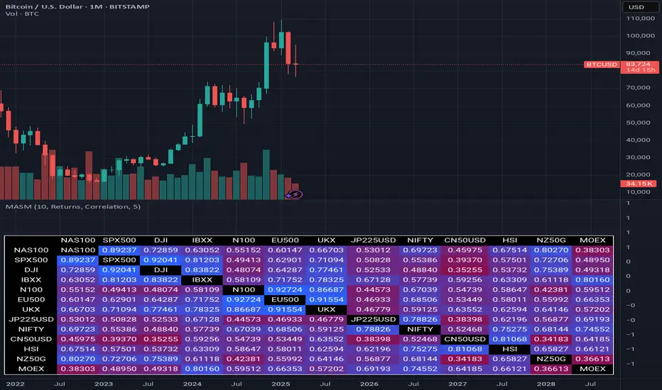
Multi Asset Similarity MatrixProvides a unique and visually stunning way to analyze the similarity between various stock market indices. This script uses a range of mathematical measures to calculate the correlation between different assets, such as indices, forex, crypto, etc..
Key Features:
Similarity Measures: The script offers a range of similarity measures to choose from, including SSD (Sum of Squared Differences), Euclidean Distance, Manhattan Distance, Minkowski Distance, Chebyshev Distance, Correlation Coefficient, Cosine Similarity, Camberra Index, Mean Absolute Error (MAE), Mean Squared Error (MSE), Lorentzian Function, Intersection, and Penrose Shape.
Asset Selection: Users can select the assets they want to analyze by entering a comma-separated list of tickers in the "Asset List" input field.
Color Gradient: The script uses a color gradient to represent the similarity values between each pair of indices, with red indicating low similarity and blue indicating high similarity.
How it Works:
The script calculates the source method (Returns or Volume Modified Returns) for each index using the sec function.
It then creates a matrix to hold the current values of each index over a specified window size (default is 10).
For each pair of indices, it applies the selected similarity measure using the select function and stores the result in a separate matrix.
The script calculates the maximum and minimum values of the similarity matrix to normalize the color gradient.
Finally, it creates a table with the index names as rows and columns, displaying the similarity values for each pair of indices using the calculated colors.
Visual Insights:
The indicator provides an intuitive way to visualize the relationships between different assets. By analyzing the color-coded tables, traders can gain insights into:
Which assets are highly correlated (blue) or uncorrelated (red)
The strength and direction of these correlations
Potential trading opportunities based on similarities and differences between assets
Overall, MASM is a powerful tool for market analysis and visualization, offering a unique perspective on the relationships between various assets.
~llama3
SPY/TLT Strategy█ STRATEGY OVERVIEW
The "SPY/TLT Strategy" is a trend-following crossover strategy designed to trade the relationship between TLT and its Simple Moving Average (SMA). The default configuration uses TLT (iShares 20+ Year Treasury Bond ETF) with a 20-period SMA, entering long positions on bullish crossovers and exiting on bearish crossunders. **This strategy is NOT optimized and performs best in trending markets.**
█ KEY FEATURES
SMA Crossover System: Uses price/SMA relationship for signal generation (Default: 20-period)
Dynamic Time Window: Configurable backtesting period (Default: 2014-2099)
Equity-Based Position Sizing: Default 100% equity allocation per trade
Real-Time Visual Feedback: Price/SMA plot with trend-state background coloring
Event-Driven Execution: Processes orders at bar close for accurate backtesting
█ SIGNAL GENERATION
1. LONG ENTRY CONDITION
TLT closing price crosses ABOVE SMA
Occurs within specified time window
Generates market order at next bar open
2. EXIT CONDITION
TLT closing price crosses BELOW SMA
Closes all open positions immediately
█ ADDITIONAL SETTINGS
SMA Period: Simple Moving Average length (Default: 20)
Start Time and End Time: The time window for trade execution (Default: 1 Jan 2014 - 1 Jan 2099)
Security Symbol: Ticker for analysis (Default: TLT)
█ PERFORMANCE OVERVIEW
Ideal Market Conditions: Strong trending environments
Potential Drawbacks: Whipsaws in range-bound markets
Backtesting results should be analyzed to optimize the MA Period and EMA Filter settings for specific instruments

TASC 2025.02 Autocorrelation Indicator█ OVERVIEW
This script implements the Autocorrelation Indicator introduced by John Ehlers in the "Drunkard's Walk: Theory And Measurement By Autocorrelation" article from the February 2025 edition of TASC's Traders' Tips . The indicator calculates the autocorrelation of a price series across several lags to construct a periodogram , which traders can use to identify market cycles, trends, and potential reversal patterns.
█ CONCEPTS
Drunkard's walk
A drunkard's walk , formally known as a random walk , is a type of stochastic process that models the evolution of a system or variable through successive random steps.
In his article, John Ehlers relates this model to market data. He discusses two first- and second-order partial differential equations, modified for discrete (non-continuous) data, that can represent solutions to the discrete random walk problem: the diffusion equation and the wave equation. According to Ehlers, market data takes on a mixture of two "modes" described by these equations. He theorizes that when "diffusion mode" is dominant, trading success is almost a matter of luck, and when "wave mode" is dominant, indicators may have improved performance.
Pink spectrum
John Ehlers explains that many recent academic studies affirm that market data has a pink spectrum , meaning the power spectral density of the data is proportional to the wavelengths it contains, like pink noise . A random walk with a pink spectrum suggests that the states of the random variable are correlated and not independent. In other words, the random variable exhibits long-range dependence with respect to previous states.
Autocorrelation function (ACF)
Autocorrelation measures the correlation of a time series with a delayed copy, or lag , of itself. The autocorrelation function (ACF) is a method that evaluates autocorrelation across a range of lags , which can help to identify patterns, trends, and cycles in stochastic market data. Analysts often use ACF to detect and characterize long-range dependence in a time series.
The Autocorrelation Indicator evaluates the ACF of market prices over a fixed range of lags, expressing the results as a color-coded heatmap representing a dynamic periodogram. Ehlers suggests the information from the periodogram can help traders identify different market behaviors, including:
Cycles : Distinguishable as repeated patterns in the periodogram.
Reversals : Indicated by sharp vertical changes in the periodogram when the indicator uses a short data length .
Trends : Indicated by increasing correlation across lags, starting with the shortest, over time.
█ USAGE
This script calculates the Autocorrelation Indicator on an input "Source" series, smoothed by Ehlers' UltimateSmoother filter, and plots several color-coded lines to represent the periodogram's information. Each line corresponds to an analyzed lag, with the shortest lag's line at the bottom of the pane. Green hues in the line indicate a positive correlation for the lag, red hues indicate a negative correlation (anticorrelation), and orange or yellow hues mean the correlation is near zero.
Because Pine has a limit on the number of plots for a single indicator, this script divides the periodogram display into three distinct ranges that cover different lags. To see the full periodogram, add three instances of this script to the chart and set the "Lag range" input for each to a different value, as demonstrated in the chart above.
With a modest autocorrelation length, such as 20 on a "1D" chart, traders can identify seasonal patterns in the price series, which can help to pinpoint cycles and moderate trends. For instance, on the daily ES1! chart above, the indicator shows repetitive, similar patterns through fall 2023 and winter 2023-2024. The green "triangular" shape rising from the zero lag baseline over different time ranges corresponds to seasonal trends in the data.
To identify turning points in the price series, Ehlers recommends using a short autocorrelation length, such as 2. With this length, users can observe sharp, sudden shifts along the vertical axis, which suggest potential turning points from upward to downward or vice versa.

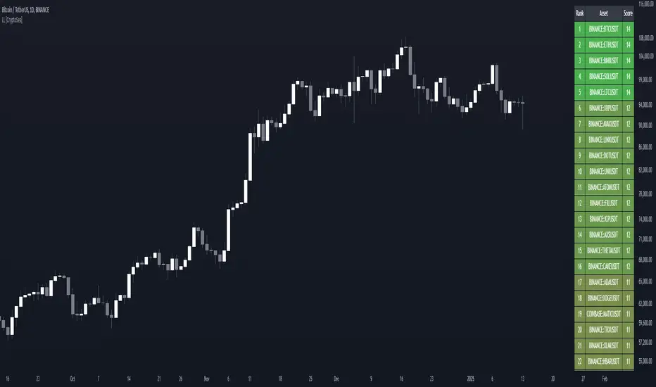
Lead-Lag Market Detector [CryptoSea]The Lead-Lag Market Detector is an advanced tool designed to help traders identify leading and lagging assets within a chosen market. This indicator leverages correlation analysis to rank assets based on their influence, making it ideal for traders seeking to optimise their portfolio or spot key market trends.
Key Features
Dynamic Asset Ranking: Utilises real-time correlation calculations to rank assets by their influence on the market, helping traders identify market leaders and laggers.
Customisable Parameters: Includes adjustable lookback periods and correlation thresholds to adapt the analysis to different market conditions and trading styles.
Comprehensive Asset Coverage: Supports up to 30 assets, offering broad market insights across cryptocurrencies, stocks, or other markets.
Gradient-Enhanced Table Display: Presents results in a colour-coded table, where assets are ranked dynamically with influence scores, aiding in quick visual analysis.
In the example below, the ranking highlights how assets tend to move in groups. For instance, BTCUSDT, ETHUSDT, BNBUSDT, SOLUSDT, and LTCUSDT are highly correlated and moving together as a group. Similarly, another group of correlated assets includes XRPUSDT, FILUSDT, APEUSDT, XTZUSDT, THETAUSDT, and CAKEUSDT. This grouping of assets provides valuable insights for traders to diversify or spread exposure.
If you believe one asset in a group is likely to perform well, you can spread your exposure into other correlated assets within the same group to capitalise on their collective movement. Additionally, assets like AVAXUSDT and ZECUSDT, which appear less correlated or uncorrelated with the rest, may offer opportunities to act as potential hedges in your trading strategy.
How it Works
Correlation-Based Scoring: Calculates pairwise correlations between assets over a user-defined lookback period, identifying assets with high influence scores as market leaders.
Customisable Thresholds: Allows traders to define a correlation threshold, ensuring the analysis focuses only on significant relationships between assets.
Dynamic Score Calculation: Scores are updated dynamically based on the timeframe and input settings, providing real-time insights into market behaviour.
Colour-Enhanced Results: The table display uses gradients to visually distinguish between leading and lagging assets, simplifying data interpretation.
Application
Portfolio Optimisation: Identifies influential assets to help traders allocate their portfolio effectively and reduce exposure to lagging assets.
Market Trend Identification: Highlights leading assets that may signal broader market trends, aiding in strategic decision-making.
Customised Trading Strategies: Adapts to various trading styles through extensive input settings, ensuring the analysis meets the specific needs of each trader.
The Lead-Lag Market Detector by is an essential tool for traders aiming to uncover market leaders and laggers, navigate complex market dynamics, and optimise their trading strategies with precision and insight.
Correlation Coefficient Master TableThe Correlation Coefficient Master Table is a comprehensive tool designed to calculate and visualize the correlation coefficient between a selected base asset and multiple other assets over various time periods. It provides traders and analysts with a clear understanding of the relationships between assets, enabling them to analyze trends, diversification opportunities, and market dynamics. You can define key parameters such as the base asset’s data source (e.g., close price), the assets to compare against (up to six symbols), and multiple lookback periods for granular analysis.
The indicator calculates the covariance and normalizes it by the product of the standard deviations. The correlation coefficient ranges from -1 to +1, with +1 indicating a perfect positive relationship, -1 a perfect negative relationship, and 0 no relationship.
You can specify the lookback periods (e.g., 15, 30, 90, or 120 bars) to tailor the calculation to their analysis needs. The results are visualized as both a line plot and a table. The line plot shows the correlation over the primary lookback period (the Chart Length), which can be used to inspect a certain length close up, or could be used in conjunction with the table to provide you with five lookback periods at once for the same base asset. The dynamically created table provides a detailed breakdown of correlation values for up to six target assets across the four user-defined lengths. The table’s cells are formatted with rounded values and color-coded for easy interpretation.
This indicator is ideal for traders, portfolio managers, and market researchers who need an in-depth understanding of asset interdependencies. By providing both the numerical correlation coefficients and their visual representation, users can easily identify patterns, assess diversification strategies, and monitor correlations across multiple timeframes, making it a valuable tool for decision-making.

S&P 500 E-Mini TrackerThis script generates a reference price for the S&P 500 ETF - SPY based on the current price of the ES contract, which is an E-Mini Futures contract representing the S&P 500 index. The indicator plots this reference price on the chart, providing a unique view of the relationship between these two popular markets.
Advantages:
Identifies divergence between the ES and SPY prices, indicating potential trading opportunities or shifts in market sentiment.
Confirms trends by showing the correlation between the ES and SPY prices.
Eliminates the need for multiple charts, allowing traders to focus on a single screen and make more informed decisions.
Customizable Parameters:
Color Scheme: Choose from various color options to customize the appearance of the indicator.
Line Style: Select from different line styles to change the visual representation of the reference price.
Divisor: Set the dividing factor to adjust the ratio at which the reference price is calculated. (Default value: 10). It is recommended to keep it at 10 for SPY.
To use it with other Stocks/ ETFs, use simple ratio math to calculate the divisor and you can customize the indicator to scale accordingly.
By using this indicator, traders can gain a deeper understanding of the relationship between the E-Mini and SPY markets, making it easier to identify trading opportunities and confirm trends.

SMT Divergence ICT 01 [TradingFinder] Smart Money Technique🔵 Introduction
SMT Divergence (short for Smart Money Technique Divergence) is a trading technique in the ICT Concepts methodology that focuses on identifying divergences between two positively correlated assets in financial markets.
These divergences occur when two assets that should move in the same direction move in opposite directions. Identifying these divergences can help traders spot potential reversal points and trend changes.
Bullish and Bearish divergences are clearly visible when an asset forms a new high or low, and the correlated asset fails to do so. This technique is applicable in markets like Forex, stocks, and cryptocurrencies, and can be used as a valid signal for deciding when to enter or exit trades.
Bullish SMT Divergence : This type of divergence occurs when one asset forms a higher low while the correlated asset forms a lower low. This divergence is typically a sign of weakness in the downtrend and can act as a signal for a trend reversal to the upside.
Bearish SMT Divergence : This type of divergence occurs when one asset forms a higher high while the correlated asset forms a lower high. This divergence usually indicates weakness in the uptrend and can act as a signal for a trend reversal to the downside.
🔵 How to Use
SMT Divergence is an analytical technique that identifies divergences between two correlated assets in financial markets.
This technique is used when two assets that should move in the same direction move in opposite directions.
Identifying these divergences can help you pinpoint reversal points and trend changes in the market.
🟣 Bullish SMT Divergence
This divergence occurs when one asset forms a higher low while the correlated asset forms a lower low. This divergence indicates weakness in the downtrend and can signal a potential price reversal to the upside.
In this case, when the correlated asset is forming a lower low, and the main asset is moving lower but the correlated asset fails to continue the downward trend, there is a high probability of a trend reversal to the upside.
🟣 Bearish SMT Divergence
Bearish divergence occurs when one asset forms a higher high while the correlated asset forms a lower high. This type of divergence indicates weakness in the uptrend and can signal a potential trend reversal to the downside.
When the correlated asset fails to make a new high, this divergence may be a sign of a trend reversal to the downside.
🟣 Confirming Signals with Correlation
To improve the accuracy of the signals, use assets with strong correlation. Forex pairs like OANDA:EURUSD and OANDA:GBPUSD , or cryptocurrencies like COINBASE:BTCUSD and COINBASE:ETHUSD , or commodities such as gold ( FX:XAUUSD ) and silver ( FX:XAGUSD ) typically have significant correlation. Identifying divergences between these assets can provide a strong signal for a trend change.
🔵 Settings
Second Symbol : This setting allows you to select another asset for comparison with the primary asset. By default, "XAUUSD" (Gold) is set as the second symbol, but you can change it to any currency pair, stock, or cryptocurrency. For example, you can choose currency pairs like EUR/USD or GBP/USD to identify divergences between these two assets.
Divergence Fractal Periods : This parameter defines the number of past candles to consider when identifying divergences. The default value is 2, but you can change it to suit your preferences. This setting allows you to detect divergences more accurately by selecting a greater number of candles.
Bullish Divergence Line : Displays a line showing bullish divergence from the lows.
Bearish Divergence Line : Displays a line showing bearish divergence from the highs.
Bullish Divergence Label : Displays the "+SMT" label for bullish divergences.
Bearish Divergence Label : Displays the "-SMT" label for bearish divergences.
🔵 Conclusion
SMT Divergence is an effective tool for identifying trend changes and reversal points in financial markets based on identifying divergences between two correlated assets. This technique helps traders receive more accurate signals for market entry and exit by analyzing bullish and bearish divergences.
Identifying these divergences can provide opportunities to capitalize on trend changes in Forex, stocks, and cryptocurrency markets. Using SMT Divergence along with risk management and confirming signals with other technical analysis tools can improve the accuracy of trading decisions and reduce risks from sudden market changes.

Correlation Confluence Trend IndicatorCorrelation Confluence Trend Indicator
Overview
The Correlation Confluence Trend Indicator combines exponential moving averages (EMAs) and statistical correlation measures to identify high-confidence trend alignments between an asset and a benchmark. By filtering signals through correlation strength, this indicator highlights opportunities when the asset and benchmark move together. In other words, it defines a trend and then uses correlation strength and the trend of a second asset to identify high-confidence trends.
Key Features
Dual EMA Trend Analysis :
Calculates fast and slow EMAs for both the asset and the selected benchmark (e.g., SPY) to identify bullish and bearish trends.
Correlation Strength Filtering :
Evaluates correlation between the asset and benchmark, identifying stronger-than-average relationships based on the mean and standard deviation.
Background Color Coding :
- Green : Strong correlation, both asset and benchmark bullish.
- Aqua : Weak correlation, both asset and benchmark bullish.
- Red : Strong correlation, both asset and benchmark bearish.
- Fuchsia : Weak correlation, both asset and benchmark bearish.
- Orange : Strong correlation, benchmark bullish, asset bearish.
- Yellow : Weak correlation, benchmark bullish, asset bearish.
- Purple : Strong correlation, benchmark bearish, asset bullish.
- Lime : Weak correlation, benchmark bearish, asset bullish.
Visual Trend Indicators :
Plots fast and slow EMAs for the asset, dynamically colored based on aggregate trend signals. The color of this corresponds to the main trend signal.
Inputs
Benchmark Symbol : Symbol of the benchmark asset to compare against.
Fast EMA Length : Period for the fast EMA calculation.
Slow EMA Length : Period for the slow EMA calculation.
Correlation Length : Number of bars for correlation calculation.
Correlation Mean Length : Number of bars for mean and standard deviation calculation.
Std Dev Multiplier : Multiplier for standard deviation to define correlation strength. When the correlation is Std Dev Multiplier standard deviations above the mean, it counts as a strong correlation.
Set Background Color : Toggle background coloring on or off.
Notes
This indicator is primarily designed for trend-following strategies. By combining trend analysis and correlation filtering, it ensures that signals occur during aligned market conditions, reducing false signals.
Before incorporating this indicator into your trading strategy:
Always backtest on historical data to evaluate its performance before committing capital.
Use proper risk management to control position sizes and mitigate potential losses.
Remember that no indicator guarantees success. I'm quite proud of this one, but it's not the holy grail.

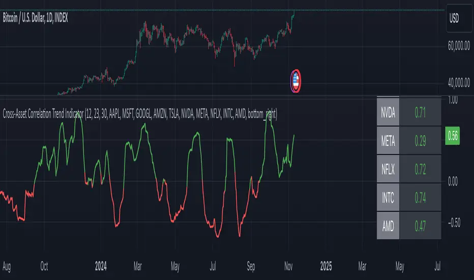
Cross-Asset Correlation Trend IndicatorCross-Asset Correlation Trend Indicator
This indicator uses correlations between the charted asset and ten others to calculate an overall trend prediction. Each ticker is configurable, and by analyzing the trend of each asset, the indicator predicts an average trend for the main asset on the chart. The strength of each asset's trend is weighted by its correlation to the charted asset, resulting in a single average trend signal. This can be a rather robust and effective signal, though it is often slow.
Functionality Overview :
The Cross-Asset Correlation Trend Indicator calculates the average trend of a charted asset based on the correlation and trend of up to ten other assets. Each asset is assigned a trend signal using a simple EMA crossover method (two customizable EMAs). If the shorter EMA crosses above the longer one, the asset trend is marked as positive; if it crosses below, the trend is negative. Each trend is then weighted by the correlation coefficient between that asset’s closing price and the charted asset’s closing price. The final output is an average weighted trend signal, which combines each trend with its respective correlation weight.
Input Parameters :
EMA 1 Length : Sets the period of the shorter EMA used to determine trends.
EMA 2 Length : Sets the period of the longer EMA used to determine trends.
Correlation Length : Defines the lookback period used for calculating the correlation between the charted asset and each of the other selected assets.
Asset Tickers : Each of the ten tickers is configurable, allowing you to set specific assets to analyze correlations with the charted asset.
Show Trend Table : Toggle to show or hide a table with each asset’s weighted trend. The table displays green, red, or white text for each weighted trend, indicating positive, negative, or neutral trends, respectively.
Table Position : Choose the position of the trend table on the chart.
Recommended Use :
As always, it’s essential to backtest the indicator thoroughly on your chosen asset and timeframe to ensure it aligns with your strategy. Feel free to modify the input parameters as needed—while the defaults work well for me, they may need adjustment to better suit your assets, timeframes, and trading style.
As always, I wish you the best of luck and immense fortune as you develop your systems. May this indicator help you make well-informed, profitable decisions!
Dynamic Market Correlation Analyzer (DMCA) v1.0Description
The Dynamic Market Correlation Analyzer (DMCA) is an advanced TradingView indicator designed to provide real-time correlation analysis between multiple assets. It offers a comprehensive view of market relationships through correlation coefficients, technical indicators, and visual representations.
Key Features
- Multi-asset correlation tracking (up to 5 symbols)
- Dynamic correlation strength categorization
- Integrated technical indicators (RSI, MACD, DX)
- Customizable visualization options
- Real-time price change monitoring
- Flexible timeframe selection
## Use Cases
1. **Portfolio Diversification**
- Identify highly correlated assets to avoid concentration risk
- Find negatively correlated assets for hedging strategies
- Monitor correlation changes during market events
2. Pairs Trading
- Detect correlation breakdowns for potential trading opportunities
- Track correlation strength for pair selection
- Monitor technical indicators for trade timing
3. Risk Management
- Assess portfolio correlation risk in real-time
- Monitor correlation shifts during market stress
- Identify potential portfolio vulnerabilities
4. **Market Analysis**
- Study sector relationships and rotations
- Analyze cross-asset correlations (e.g., stocks vs. commodities)
- Track market regime changes through correlation patterns
Components
Input Parameters
- **Timeframe**: Custom timeframe selection for analysis
- **Length**: Correlation calculation period (default: 20)
- **Source**: Price data source selection
- **Symbol Selection**: Up to 5 customizable symbols
- **Display Options**: Table position, text color, and size settings
Technical Indicators
1. **Correlation Coefficient**
- Range: -1 to +1
- Strength categories: Strong/Moderate/Weak (Positive/Negative)
2. **RSI (Relative Strength Index)**
- 14-period default setting
- Momentum comparison across assets
3. **MACD (Moving Average Convergence Divergence)**
- Standard settings (12, 26, 9)
- Trend direction indicator
4. **DX (Directional Index)**
- Trend strength measurement
- Based on DMI calculations
Visual Components
1. **Correlation Table**
- Symbol identifiers
- Correlation coefficients
- Correlation strength descriptions
- Price change percentages
- Technical indicator values
2. **Correlation Plot**
- Real-time correlation visualization
- Multiple correlation lines
- Reference levels at -1, 0, and +1
- Color-coded for easy identification
Installation and Setup
1. Load the indicator on TradingView
2. Configure desired symbols (up to 5)
3. Adjust timeframe and calculation length
4. Customize display settings
5. Enable/disable desired components (table, plot, RSI)
Best Practices
1. **Symbol Selection**
- Choose related but distinct assets
- Include a mix of asset classes
- Consider market cap and liquidity
2. **Timeframe Selection**
- Match timeframe to trading strategy
- Consider longer timeframes for strategic analysis
- Use shorter timeframes for tactical decisions
3. **Interpretation**
- Monitor correlation changes over time
- Consider multiple timeframes
- Combine with other technical analysis tools
- Account for market conditions and volatility
Performance Notes
- Calculations update in real-time
- Resource usage scales with number of active symbols
- Historical data availability may affect initial calculations
Version History
- v1.0: Initial release with core functionality
- Multi-symbol correlation analysis
- Technical indicator integration
- Customizable display options
Future Enhancements (Planned)
- Additional technical indicators
- Advanced correlation algorithms
- Enhanced visualization options
- Custom alert conditions
- Statistical significance testing

[ AlgoChart ] - Pearson Index CorrelationCorrelation Indicator (Pearson Index)
The correlation indicator measures the strength and direction of the relationship between two financial assets using the Pearson Index.
Correlation values range from +100 to -100, where:
+100 indicates perfect positive correlation, meaning the two assets tend to move in the same direction.
-100 indicates perfect negative correlation, where the two assets move in opposite directions.
The neutral zone ranges from +25% to -25%, suggesting that the asset movements are independent, with no clear correlation between them.
Interpreting Correlation Levels:
Correlation above +75%: The two assets tend to move similarly and in the same direction. This may indicate a risk of overexposure if both assets are traded in the same direction, as their movements will be very similar, increasing the likelihood of double losses or gains.
Correlation below -75%: The two assets tend to move similarly but in opposite directions. This correlation level can be useful for strategies that benefit from opposing movements between assets, such as trading pairs with inverse dynamics.
Practical Use of the Indicator:
Risk management: Use the indicator to monitor asset correlations before opening positions. High correlation may indicate you are duplicating exposure, as two highly correlated assets tend to move similarly. This helps avoid excessive risk and improves portfolio diversification.
Statistical Arbitrage: During moments of temporary decorrelation between two assets, the indicator can be used for statistical arbitrage strategies. In such cases, you can take advantage of the divergence by opening positions and closing them when the correlation returns to higher or positive levels, thus potentially profiting from the reconvergence of movements.
While the correlation indicator provides valuable insights into asset relationships, it is most effective when used in conjunction with other concepts and tools. On its own, it may offer limited relevance in trading decisions.
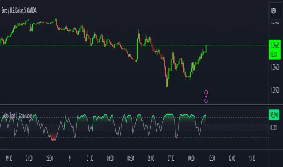
TechniTrend: Dynamic Pair CorrelationTechniTrend: Dynamic Pair Correlation
Description:
The TechniTrend: Dynamic Pair Correlation is a powerful and versatile indicator designed to track the correlation between two assets—whether cryptocurrencies, indices, or other financial instruments—across multiple timeframes. Understanding correlations can provide deep insights into market behavior, helping traders make informed decisions based on how two assets move in relation to each other.
Key Features:
Customizable Pair Selection: Compare any two assets (e.g., Bitcoin and DXY, Ethereum and SP500) to study how their price movements relate over time.
Multi-Timeframe Analysis: Simultaneously track correlations across different timeframes—standard, lower, and higher—providing a comprehensive view of market dynamics.
Dynamic Color Coding for Correlation Strength: Instantly spot correlations with visually intuitive colors—green for strong positive correlation, red for strong negative correlation, and yellow for neutral.
Heatmap Background: An easy-to-read background color heatmap highlights when correlations hit extreme levels, adding another layer of insight to your charts.
Real-Time Alerts: Get notified when correlations exceed your custom thresholds, signaling opportunities for potential breakouts, reversals, or divergences.
Divergence Detection: Automatically highlight moments when asset prices diverge, offering potential entry/exit points for smart trading decisions.
How to Use:
Asset Pair Comparison: Select two symbols to analyze their price correlation, such as BTC/USDT and DXY, or any other pair that fits your strategy.
Set Your Timeframes: Customize your standard, lower, and higher timeframes to monitor correlations at different intervals, allowing you to capture both short-term and long-term relationships.
Track Correlation Strength: Use dynamic color coding to quickly see how closely two assets are moving together. Strong correlations (positive or negative) could signal potential opportunities, while low correlations may indicate the absence of a strong trend.
Utilize Alerts: Receive real-time alerts when correlations cross your predefined thresholds, helping you take action when the market presents strong alignment or divergence.
Divergence Signals: Watch for divergence between the assets on multiple timeframes, which could indicate a potential trend reversal or a shift in market behavior.
Why It’s Essential:
Understanding the relationship between two assets can be a game changer for traders. Whether you're comparing Bitcoin to DXY, tracking the correlation between Ethereum and major indices, or evaluating two cryptocurrencies, this indicator gives you the tools to visualize and respond to market conditions with precision.
Perfect For:
Crypto traders looking to optimize strategies by monitoring the relationship between major cryptocurrencies and other assets.
Arbitrageurs seeking to capitalize on temporary pricing anomalies between correlated pairs.
Trend-followers aiming to catch large movements by detecting alignment or divergence between asset classes.
Portfolio managers monitoring how different asset classes impact each other to hedge or diversify investments.
By leveraging the TechniTrend: Dynamic Pair Correlation indicator, traders can gain deeper insights into market trends, correlations, and divergences, giving them an edge in fast-moving markets.
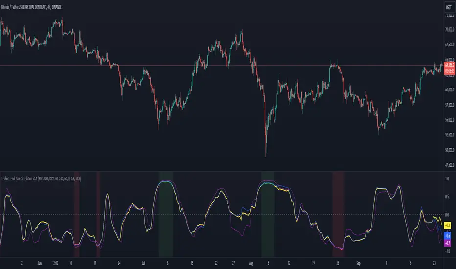
Correlation Clusters [LuxAlgo]The Correlation Clusters is a machine learning tool that allows traders to group sets of tickers with a similar correlation coefficient to a user-set reference ticker.
The tool calculates the correlation coefficients between 10 user-set tickers and a user-set reference ticker, with the possibility of forming up to 10 clusters.
🔶 USAGE
Applying clustering methods to correlation analysis allows traders to quickly identify which set of tickers are correlated with a reference ticker, rather than having to look at them one by one or using a more tedious approach such as correlation matrices.
Tickers belonging to a cluster may also be more likely to have a higher mutual correlation. The image above shows the detailed parts of the Correlation Clusters tool.
The correlation coefficient between two assets allows traders to see how these assets behave in relation to each other. It can take values between +1.0 and -1.0 with the following meaning
Value near +1.0: Both assets behave in a similar way, moving up or down at the same time
Value close to 0.0: No correlation, both assets behave independently
Value near -1.0: Both assets have opposite behavior when one moves up the other moves down, and vice versa
There is a wide range of trading strategies that make use of correlation coefficients between assets, some examples are:
Pair Trading: Traders may wish to take advantage of divergences in the price movements of highly positively correlated assets; even highly positively correlated assets do not always move in the same direction; when assets with a correlation close to +1.0 diverge in their behavior, traders may see this as an opportunity to buy one and sell the other in the expectation that the assets will return to the likely same price behavior.
Sector rotation: Traders may want to favor some sectors that are expected to perform in the next cycle, tracking the correlation between different sectors and between the sector and the overall market.
Diversification: Traders can aim to have a diversified portfolio of uncorrelated assets. From a risk management perspective, it is useful to know the correlation between the assets in your portfolio, if you hold equal positions in positively correlated assets, your risk is tilted in the same direction, so if the assets move against you, your risk is doubled. You can avoid this increased risk by choosing uncorrelated assets so that they move independently.
Hedging: Traders may want to hedge positions with correlated assets, from a hedging perspective, if you are long an asset, you can hedge going long a negatively correlated asset or going short a positively correlated asset.
Grouping different assets with similar behavior can be very helpful to traders to avoid over-exposure to those assets, traders may have multiple long positions on different assets as a way of minimizing overall risk when in reality if those assets are part of the same cluster traders are maximizing their risk by taking positions on assets with the same behavior.
As a rule of thumb, a trader can minimize risk via diversification by taking positions on assets with no correlations, the proposed tool can effectively show a set of uncorrelated candidates from the reference ticker if one or more clusters centroids are located near 0.
🔶 DETAILS
K-means clustering is a popular machine-learning algorithm that finds observations in a data set that are similar to each other and places them in a group.
The process starts by randomly assigning each data point to an initial group and calculating the centroid for each. A centroid is the center of the group. K-means clustering forms the groups in such a way that the variances between the data points and the centroid of the cluster are minimized.
It's an unsupervised method because it starts without labels and then forms and labels groups itself.
🔹 Execution Window
In the image above we can see how different execution windows provide different correlation coefficients, informing traders of the different behavior of the same assets over different time periods.
Users can filter the data used to calculate correlations by number of bars, by time, or not at all, using all available data. For example, if the chart timeframe is 15m, traders may want to know how different assets behave over the last 7 days (one week), or for an hourly chart set an execution window of one month, or one year for a daily chart. The default setting is to use data from the last 50 bars.
🔹 Clusters
On this graph, we can see different clusters for the same data. The clusters are identified by different colors and the dotted lines show the centroids of each cluster.
Traders can select up to 10 clusters, however, do note that selecting 10 clusters can lead to only 4 or 5 returned clusters, this is caused by the machine learning algorithm not detecting any more data points deviating from already detected clusters.
Traders can fine-tune the algorithm by changing the 'Cluster Threshold' and 'Max Iterations' settings, but if you are not familiar with them we advise you not to change these settings, the defaults can work fine for the application of this tool.
🔹 Correlations
Different correlations mean different behaviors respecting the same asset, as we can see in the chart above.
All correlations are found against the same asset, traders can use the chart ticker or manually set one of their choices from the settings panel. Then they can select the 10 tickers to be used to find the correlation coefficients, which can be useful to analyze how different types of assets behave against the same asset.
🔶 SETTINGS
Execution Window Mode: Choose how the tool collects data, filter data by number of bars, time, or no filtering at all, using all available data.
Execute on Last X Bars: Number of bars for data collection when the 'Bars' execution window mode is active.
Execute on Last: Time window for data collection when the `Time` execution window mode is active. These are full periods, so `Day` means the last 24 hours, `Week` means the last 7 days, and so on.
🔹 Clusters
Number of Clusters: Number of clusters to detect up to 10. Only clusters with data points are displayed.
Cluster Threshold: Number used to compare a new centroid within the same cluster. The lower the number, the more accurate the centroid will be.
Max Iterations: Maximum number of calculations to detect a cluster. A high value may lead to a timeout runtime error (loop takes too long).
🔹 Ticker of Reference
Use Chart Ticker as Reference: Enable/disable the use of the current chart ticker to get the correlation against all other tickers selected by the user.
Custom Ticker: Custom ticker to get the correlation against all the other tickers selected by the user.
🔹 Correlation Tickers
Select the 10 tickers for which you wish to obtain the correlation against the reference ticker.
🔹 Style
Text Size: Select the size of the text to be displayed.
Display Size: Select the size of the correlation chart to be displayed, up to 500 bars.
Box Height: Select the height of the boxes to be displayed. A high height will cause overlapping if the boxes are close together.
Clusters Colors: Choose a custom colour for each cluster.
