Has Bitcoin Reached It's Four-Year Cycle Top?Why Bitcoin Might Have Reached Its Four-Year Cycle Top
Historical Pattern: Bitcoin's four-year cycle often peaks around halving events, influencing supply and price dynamics.
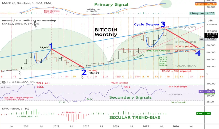
MACD Signal: The primary signal indicator in the upper panel remains in a bullish position, with no bearish cross, indicating ongoing upward momentum.
Wave 3 Peak: The current print high of 125,417 USD marks the crest of Cycle Degree 3, the strongest wave in an impulse sequence.
Elliott Wave Count Analysis
Current Position: The chart labels the all-time print high of the Cycle Degree 3 high at 125,417.
Wave 4 Expectation: A corrective wave 4 decline is anticipated, but it must remain above the wave one high of 69,000 USD to uphold the Elliott Wave structure.
Wave 5 Potential: If wave 4 holds above 69,000 USD, a subsequent wave 5 could drive prices far higher, completing a larger Super Cycle degree wave I.
Bullish Posture and Key Levels
Primary Signal Indicator: The long-term bullish posture based on the MACD remains intact, with the indicator staying bullish until a monthly close shows the fast-moving average crossing and closing below the slow-moving average.
Support Level: Maintaining above 69,000 USD during any wave 4 pullback is crucial for the long-term bullish posture to persist and conform with the current wave count analysis.
Community ideas
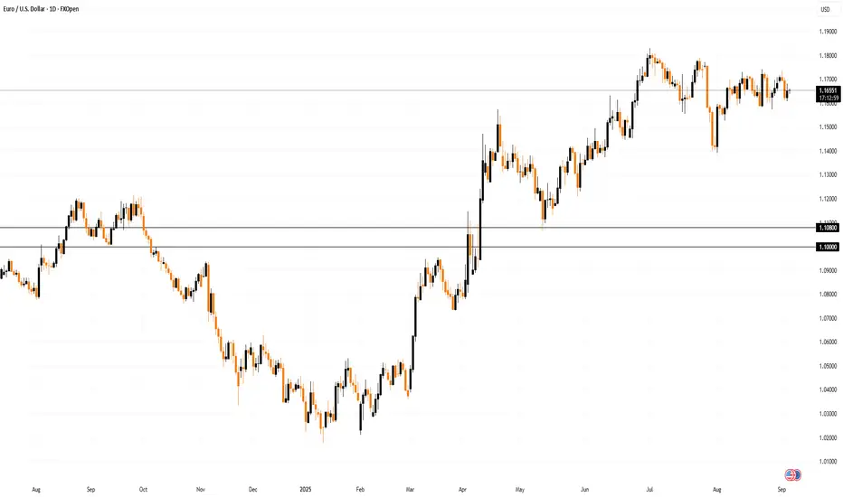
Indecision - The Human Experience of Being A DojiContext : Daily Chart ETHUSD.
Uptrend intact.
Price sitting right on the trend line.
Price consolidating into a series of dojis.
Imagine this scenario.
You have a plan.
You're a trend trader.
You're looking to get long.
You start to observe the context…
We’re into September.
Tech showing signs of correcting.
Gold heading up.
This chart... right here, right now is consolidating.
And so you experience a little flicker.
A small niggle …
There it is.
The voice of doubt.
"I should get long but maybe this is the one that gives way".
You feel a moment of indecision.
And you’re stuck frozen
The human version of a doji.
Indecision has a cost and takes a toll.
Not just in lost opportunity BUT in energy and confidence.
A simple practice to help guard against this:
Pre-decide the conditions.
Write down before you enter what tells you to stay in and what tells you to step aside.
Separate the signal from the noise.
Notice the flicker of doubt, but act on your plan, not the passing thought.
Doubt will always show up.
The edge comes from knowing what you’ll do when it does.

Weierstrass Function: Fractal Cycles🏛️ RESEARCH NOTES
In financial markets, asset prices move in broken waves, seemingly random patterns because they reflect the decentralized and often conflicting decisions of countless participants. No single force dictates this behavior; it emerges from the collective actions of millions acting on different information and expectations. Constantly shifting news and uncertainty cause prices to fluctuate like a stochastic process, similar to Brownian motion. These fluctuations stem from past events, current news, and future speculation often disconnected from fundamentals - and would stabilize only if all outcomes were perfectly known in advance.
Given that markets function as emergent systems in which order develops from iterative interaction cycles, I consider its raw geometry a necessary approach for advancing a more precise understanding of price dynamics as expressed in their behavior.
🇩🇪 The Weierstrass Function is a classic example of a "fractal curve", as it is continuous and is nowhere differentiable. This means it is infinitely jagged at every single point, so regardless the zoom, it never becomes smooth. Similarly, in markets, the large cycles contain medium cycles, which further scale down to nested micro-cycles.
f(x) = ∑(n=0)^∞ a^n * cos(b^n * π * x)
a^n → ensures higher-frequency components have smaller amplitude, keeping the series bounded.
b^n → scales the frequency, creating finer oscillations that nest inside larger cycles.
N (n_terms) → truncates the infinite sum to a practical number of terms.
Scale_factor → maps the abstract mathematical domain to the time axis of the price chart.
❖ Shapes of Fractal Cycles
With default parameters, the function reproduces the characteristic roughness it is known for.
At a frequency factor of 5, nested cycles are compressed along the time axis, while the frequency and magnitude of reversals increase. The resulting structure closely resembles Elliott wave patterns.
At a frequency factor of 9, composite cycles emerge at smaller scales. The steep angles cause movements to unfold as rapid but short-lived spikes.
At extreme values (e.g., frequency factor >1000), cycles overlap extensively, producing dense interference patterns with significant stretching and deformation.
❗️Each added term does not “react” to price. Instead, it generates a composite waveform in which multiple cycles are naturally nested. The resulting fractal wave is topologically organized, meaning it encodes trends of different scales in one structure without any bias toward trend-following.
The Weierstrass function is a generative fractal model that builds waves nested across multiple scales. It doesn’t react to market data but provides a topological view of trend structure, showing how cycles naturally scale and interlock instead of prescribing signals.

Role of Rating Agencies in Global Capital FlowsIntroduction
Global capital flows—the cross-border movement of financial resources in the form of equity, debt, and investments—are a critical element of the modern financial system. They connect savings from one part of the world to investment opportunities in another, enabling economic growth, diversification of risk, and efficient allocation of capital. However, capital flows are also influenced by perceptions of creditworthiness, risk, and trust in financial systems. This is where credit rating agencies (CRAs) play a decisive role.
Credit rating agencies such as Standard & Poor’s (S&P), Moody’s, and Fitch Ratings have become central arbiters in the global financial marketplace. Their ratings on sovereigns, corporations, and structured financial products serve as signals of risk that investors use when making cross-border investment decisions. From setting borrowing costs to influencing capital allocation, rating agencies have profound power in shaping the direction, volume, and cost of global capital flows.
This essay explores in detail the role of rating agencies in global capital flows, their mechanisms, benefits, criticisms, historical case studies, and the way forward in ensuring accountability and stability in global markets.
1. Understanding Credit Rating Agencies
1.1 Definition and Function
Credit rating agencies are private institutions that assess the creditworthiness of borrowers—whether sovereign governments, financial institutions, corporations, or structured products like mortgage-backed securities. A credit rating expresses the likelihood that the borrower will meet its financial obligations on time.
Investment-grade ratings (e.g., AAA, AA, A, BBB) suggest relatively low risk.
Speculative or junk ratings (BB, B, CCC, etc.) indicate higher risk.
1.2 Types of Ratings
Sovereign Ratings: Evaluate a country’s ability and willingness to repay debt.
Corporate Ratings: Assess credit quality of companies.
Structured Finance Ratings: Evaluate securities backed by assets (mortgages, loans, etc.).
1.3 Market Power of CRAs
Ratings are widely used because:
Institutional investors (pension funds, insurance companies, mutual funds) are often restricted by regulations to invest only in investment-grade securities.
Ratings influence risk premiums, spreads, and interest rates.
Global organizations like the IMF and World Bank rely on ratings for policy design and lending frameworks.
Thus, CRAs act as gatekeepers of global capital flows, determining which entities can access international markets and at what cost.
2. Role of Rating Agencies in Global Capital Flows
2.1 Facilitating Capital Allocation
In an interconnected financial system, investors require credible signals about where to allocate capital. Rating agencies reduce information asymmetry between borrowers and lenders by providing standardized risk assessments. For example:
A pension fund in Canada may consider investing in bonds issued by an infrastructure company in India. Without ratings, assessing risk across borders would be complex.
Ratings provide a benchmark for investors who may lack detailed knowledge about local markets.
2.2 Determining Borrowing Costs
Ratings directly impact interest rates.
A sovereign with an AAA rating can borrow internationally at very low interest rates.
Conversely, a country downgraded to “junk” status faces higher costs and reduced investor appetite.
Example: Greece’s sovereign debt crisis (2010–2012) showed how downgrades led to skyrocketing bond yields and loss of market access.
2.3 Shaping Sovereign Debt Markets
Sovereign ratings are crucial for emerging and developing economies seeking external financing. They:
Influence foreign direct investment (FDI) and portfolio inflows.
Affect perceptions of political stability and governance.
Serve as benchmarks for corporate borrowers in the same country.
If a sovereign rating is downgraded, often domestic corporations are automatically penalized since their creditworthiness is tied to the country’s risk profile.
2.4 Impact on Capital Market Development
Rating agencies encourage capital market deepening by:
Providing credible assessments that attract foreign investors.
Supporting development of local bond markets by setting credit benchmarks.
Enabling securitization and structured finance.
For example, Asian countries after the 1997–98 financial crisis used sovereign ratings to attract stable international capital for infrastructure financing.
2.5 Acting as “Gatekeepers” in Global Finance
Because many regulatory frameworks link investment eligibility to ratings, CRAs effectively decide who can tap global pools of capital.
A downgrade below investment grade can trigger forced selling by institutional investors.
Upgrades attract capital inflows by expanding the base of eligible investors.
Thus, they not only influence prices but also capital mobility across borders.
3. Case Studies on Ratings and Capital Flows
3.1 Asian Financial Crisis (1997–98)
Before the crisis, CRAs maintained relatively favorable ratings for Asian economies despite growing imbalances. When the crisis erupted, they issued sharp downgrades, accelerating capital flight.
Criticism: Ratings were lagging indicators rather than predictors.
Impact: Countries like Thailand, Indonesia, and South Korea saw capital outflows magnified by sudden rating downgrades.
3.2 Argentina Debt Crisis (2001 & 2018)
Argentina’s sovereign debt rating was repeatedly downgraded during its fiscal crisis, pushing borrowing costs higher.
Investors pulled out en masse after downgrades to junk status.
Access to international markets dried up, forcing defaults.
3.3 Eurozone Debt Crisis (2010–2012)
Countries like Greece, Portugal, and Ireland experienced downgrades that worsened their debt sustainability.
Rating actions led to a self-fulfilling prophecy: downgrades → higher borrowing costs → deeper fiscal distress.
EU regulators accused CRAs of procyclicality, meaning they intensified crises instead of stabilizing markets.
3.4 Subprime Mortgage Crisis (2007–2008)
CRAs assigned high ratings to mortgage-backed securities (MBS) that later collapsed.
Resulted in massive misallocation of global capital.
Global investors trusted AAA-rated securities that were actually risky.
This highlighted the conflict of interest in the “issuer-pays” model, where companies pay for their own ratings.
4. Benefits of Rating Agencies in Capital Flows
Reduce Information Asymmetry: Provide standardized, comparable measures of risk.
Enable Cross-Border Investment: Facilitate capital flows by offering risk assessments across jurisdictions.
Support Market Liquidity: Ratings enhance tradability of securities by offering confidence to investors.
Encourage Market Discipline: Poor governance or weak policies may be punished with downgrades, pressuring governments to maintain sound macroeconomic frameworks.
Benchmarking Role: Provide reference points for pricing bonds, derivatives, and risk models.
5. Criticisms and Challenges
5.1 Procyclicality
CRAs often amplify financial cycles.
During booms, they assign excessively high ratings, encouraging inflows.
During downturns, they downgrade abruptly, worsening outflows.
5.2 Conflicts of Interest
The issuer-pays model creates bias: issuers pay CRAs for ratings, leading to inflated assessments.
5.3 Over-Reliance by Regulators
International financial regulations (e.g., Basel Accords) embed credit ratings into capital requirements. This gives CRAs outsized influence and encourages investors to rely uncritically on ratings.
5.4 Lack of Transparency
Methodologies are often opaque, making it difficult to understand rating decisions.
5.5 Geopolitical Bias
Emerging economies often argue that rating agencies, largely based in the US and Europe, display Western bias, leading to harsher ratings compared to developed economies with similar fundamentals.
5.6 Systemic Risks
Errors in ratings can misallocate trillions of dollars in global capital. The 2008 crisis is the most striking example.
6. Regulatory Reforms and Alternatives
6.1 Post-2008 Reforms
Dodd-Frank Act (US): Reduced regulatory reliance on ratings.
European Union: Increased supervision of CRAs via the European Securities and Markets Authority (ESMA).
IOSCO Principles: Set global standards for transparency, governance, and accountability.
6.2 Calls for Diversification
Development of regional rating agencies (e.g., China’s Dagong Global).
Use of market-based indicators (bond spreads, CDS prices) as complements to ratings.
Encouraging investor due diligence instead of blind reliance.
6.3 Technological Alternatives
Use of big data analytics and AI-driven credit assessment.
Decentralized financial platforms may reduce reliance on centralized CRAs.
7. The Way Forward
Balanced Role: CRAs should provide guidance without becoming the sole determinants of capital flows.
Greater Accountability: Legal and regulatory frameworks must hold rating agencies responsible for negligence or misconduct.
Enhanced Transparency: Methodologies and assumptions should be disclosed to prevent opaque judgments.
Diversification of Voices: Regional agencies and independent research firms should complement dominant players.
Investor Education: Encouraging critical evaluation rather than over-reliance on ratings.
Conclusion
Credit rating agencies hold immense power over global capital flows. Their assessments determine borrowing costs, investor confidence, and even the economic destiny of nations. On the positive side, they reduce information asymmetry, facilitate cross-border investment, and provide benchmarks for global markets. On the negative side, their procyclicality, conflicts of interest, and opaque methodologies have at times worsened financial crises and distorted capital allocation.
The history of financial crises from Asia in 1997 to the subprime meltdown in 2008 illustrates both the necessity and the dangers of CRAs. While reforms have sought to improve accountability and transparency, the global financial system remains deeply influenced by their ratings.
The way forward lies in diversification of risk assessment mechanisms, greater transparency, and reduced regulatory over-reliance on CRAs. In doing so, global capital flows can be guided more efficiently, fairly, and sustainably, ensuring that they support economic growth rather than exacerbate instability.

Global Agricultural Commodities MarketWhat Are Agricultural Commodities?
Agricultural commodities are raw, unprocessed products grown or raised to be sold or exchanged. They fall broadly into two categories:
Food Commodities
Grains & cereals: Wheat, rice, maize, barley, oats.
Oilseeds: Soybeans, rapeseed, sunflower, groundnut.
Fruits & vegetables: Bananas, citrus, potatoes, onions.
Livestock & animal products: Beef, pork, poultry, dairy, eggs.
Tropical commodities: Coffee, cocoa, tea, sugar.
Non-Food Commodities
Fibers: Cotton, jute, wool.
Biofuel crops: Corn (ethanol), sugarcane (ethanol), palm oil, soy oil (biodiesel).
Industrial crops: Rubber, tobacco.
These commodities are traded on spot markets (immediate delivery) and futures markets (contracts for future delivery). Futures trading, which developed in places like Chicago and London, allows farmers and buyers to hedge against price fluctuations.
Historical Context of Agricultural Commodities Trade
Ancient Trade: The Silk Road and spice trade routes included agricultural goods like rice, spices, and tea. Grain storage and trade were central to the Roman Empire and ancient Egypt.
Colonial Era: European colonial powers built empires around commodities like sugar, cotton, tobacco, and coffee.
20th Century: Mechanization, the Green Revolution, and globalization expanded agricultural production and trade.
21st Century: Digital platforms, biotechnology, and sustainability initiatives shape modern agricultural commodity markets.
This long history shows how agriculture is not just economic, but political and cultural.
Key Players in the Global Agricultural Commodities Market
Producers (Farmers & Agribusinesses): Smallholder farmers in Asia and Africa; large-scale industrial farms in the U.S., Brazil, and Australia.
Traders & Merchants: Multinational corporations known as the ABCD companies—Archer Daniels Midland (ADM), Bunge, Cargill, and Louis Dreyfus—dominate global grain and oilseed trade.
Governments & Agencies: World Trade Organization (WTO), Food and Agriculture Organization (FAO), national agricultural boards.
Financial Institutions & Exchanges: Chicago Board of Trade (CBOT), Intercontinental Exchange (ICE), and hedge funds/speculators who trade futures.
Consumers & Industries: Food processing companies, retailers, biofuel producers, and ultimately, households.
Major Agricultural Commodities and Their Markets
1. Cereals & Grains
Wheat: Staple for bread and pasta, major producers include Russia, the U.S., Canada, and India.
Rice: Lifeline for Asia; grown largely in China, India, Thailand, and Vietnam.
Corn (Maize): Used for food, feed, and ethanol; U.S. and Brazil dominate exports.
2. Oilseeds & Oils
Soybeans: Key protein for animal feed; U.S., Brazil, and Argentina lead.
Palm Oil: Major in Indonesia and Malaysia; used in food and cosmetics.
Sunflower & Rapeseed Oil: Important in Europe, Ukraine, and Russia.
3. Tropical Commodities
Coffee: Produced mainly in Brazil, Vietnam, Colombia, and Ethiopia.
Cocoa: Critical for chocolate; grown in West Africa (Ivory Coast, Ghana).
Sugar: Brazil, India, and Thailand dominate.
4. Livestock & Dairy
Beef & Pork: U.S., Brazil, China, and EU major players.
Poultry: Fastest-growing meat sector, strong in U.S. and Southeast Asia.
Dairy: New Zealand, EU, and India lead in milk and milk powder exports.
5. Fibers & Industrial Crops
Cotton: Vital for textiles; India, U.S., and China are leading producers.
Rubber: Largely grown in Southeast Asia for tires and industrial use.
Factors Influencing Agricultural Commodity Markets
Weather & Climate: Droughts, floods, hurricanes, and heatwaves strongly affect supply.
Technology: Mechanization, biotechnology (GM crops), digital farming, and precision agriculture boost productivity.
Geopolitics: Wars, sanctions, and trade disputes disrupt supply chains (e.g., Russia-Ukraine war and wheat exports).
Currency Fluctuations: Commodities are priced in USD; exchange rates impact competitiveness.
Government Policies: Subsidies, tariffs, price supports, and export bans affect markets.
Consumer Demand: Rising demand for protein, organic food, and biofuels shapes production.
Speculation: Futures and derivatives markets amplify price volatility.
Supply Chain of Agricultural Commodities
Production (Farmers).
Collection (Local traders & cooperatives).
Processing (Milling, crushing, refining).
Storage & Transportation (Warehouses, silos, shipping lines).
Trading & Export (Grain merchants, commodity exchanges).
Retail & Consumption (Supermarkets, restaurants, households).
The supply chain is global—soybeans grown in Brazil may feed livestock in China, which supplies meat to Europe.
Global Trade in Agricultural Commodities
Top Exporters: U.S., Brazil, Argentina, Canada, EU, Australia.
Top Importers: China, India, Japan, Middle East, North Africa.
Trade Routes: Panama Canal, Suez Canal, Black Sea, and major ports like Rotterdam, Shanghai, and New Orleans.
Agricultural trade is often uneven—developed nations dominate exports, while developing nations rely heavily on imports.
Price Volatility in Agricultural Commodities
Agricultural commodities are highly volatile due to:
Seasonal cycles of planting and harvest.
Weather shocks (El Niño, La Niña).
Energy prices (fertilizers, transport).
Speculative trading on futures markets.
Volatility impacts both farmers’ incomes and consumers’ food security.
Role of Futures and Derivatives Markets
Commodity exchanges such as CBOT (Chicago), ICE (New York), and NCDEX (India) allow:
Hedging: Farmers and buyers reduce risk by locking in prices.
Speculation: Traders bet on price movements, adding liquidity but also volatility.
Price Discovery: Futures prices signal supply-demand trends.
Challenges Facing the Global Agricultural Commodities Market
Climate Change: Increased droughts, floods, and pests reduce yields.
Food Security: Rising global population (10 billion by 2050) requires 50% more food production.
Trade Wars & Protectionism: Export bans (e.g., rice from India, wheat from Russia) destabilize markets.
Sustainability: Deforestation for soy and palm oil, pesticide use, and water scarcity are major concerns.
Market Power Concentration: Few large corporations dominate, raising fairness concerns.
Infrastructure Gaps: Poor roads, ports, and storage in developing nations lead to waste.
Future Trends in Agricultural Commodities Market
Sustainability & ESG: Demand for eco-friendly, deforestation-free, and fair-trade commodities.
Digitalization: Blockchain for traceability, AI for crop forecasting, precision farming.
Biofuels & Renewable Energy: Growing role of corn, sugarcane, and soy in energy transition.
Alternative Proteins: Lab-grown meat, plant-based proteins reducing demand for livestock feed.
Regional Shifts: Africa emerging as a key producer and consumer market.
Climate-Resilient Crops: GM crops resistant to drought, pests, and diseases.
Case Studies
Russia-Ukraine War (2022–2025): Disrupted global wheat, corn, and sunflower oil supply, driving food inflation.
COVID-19 Pandemic (2020): Supply chain breakdowns exposed vulnerabilities in agricultural trade.
Palm Oil in Indonesia: Tensions between economic growth and environmental concerns over deforestation.
Conclusion
The global agricultural commodities market is one of the most important pillars of the world economy. It determines food security, influences geopolitics, and drives livelihoods for billions of farmers. However, it is also one of the most vulnerable markets—shaped by climate change, population growth, technological advances, and political instability.
In the future, balancing food security, sustainability, and fair trade will be the central challenge. With the right policies, innovation, and cooperation, agricultural commodity markets can continue to feed the world while protecting the planet.

What Is the ARIMA Prediction Model?What Is the ARIMA Prediction Model?
ARIMA (autoregressive integrated moving average) is a statistical model used to analyse time series data, making it a popular tool in financial markets. Traders apply ARIMA to assess historical price trends and identify structured patterns in market movements. This article explains how ARIMA works, its strengths and limitations, and how it can be integrated into trading strategies for a deeper analysis of price behaviour across different assets.
Understanding ARIMA
ARIMA stands for autoregressive integrated moving average, a widely used model for analysing time series data. It’s particularly useful in financial markets because it helps traders break down price movements into patterns based on historical data. To understand how ARIMA works, it’s important to look at its three components:
- Autoregressive (AR): This part captures the relationship between a current value and its past values. For example, if the price of an asset today is influenced by its price over the last few days, that’s an autoregressive process.
- Integrated (I): Many financial time series exhibit trends, making them non-stationary (meaning their statistical properties change over time). ARIMA “integrates” the data by differencing it—subtracting past values from current ones—to make it more stable for analysis.
- Moving Average (MA): Instead of focusing on past prices, this component looks at past errors—how much previous values deviated from expected trends—to refine the analysis.
Each ARIMA model is defined by three parameters: p (AR order), d (number of differences), and q (MA order). Selecting these values requires statistical tests, autocorrelation analysis, and model evaluation methods like the Akaike Information Criterion (AIC).
In practice, ARIMA modelling is often used in trading to analyse historical price trends and identify repeating patterns.
How ARIMA Works in Market Analysis
Applying ARIMA to financial markets involves a structured process that helps traders analyse price movements based on historical patterns. Since markets generate continuous time series data—such as stock prices, forex rates, and commodity values—ARIMA can be used to extract meaningful trends from past performance. However, applying ARIMA to a time series isn’t done blindly; there are key steps analysts follow to try to improve its effectiveness.
1. Checking for Stationarity
Most raw financial data isn’t stationary—it often trends upwards or downwards over time. ARIMA requires stationarity, meaning that statistical properties like mean and variance remain constant. Traders test for this using the Augmented Dickey-Fuller (ADF) test. If the data is non-stationary, differencing (subtracting previous values from current values) is applied until stationarity is achieved.
2. Identifying AR and MA Components
Once the data is stationary, traders determine how much past price data (AR) and past errors (MA) influence current values. This is done using Autocorrelation Functions (ACF) and Partial Autocorrelation Functions (PACF):
- ACF measures how strongly past values are correlated with present values.
- PACF isolates the direct relationship between a value and its past lags, ignoring indirect effects.
These tools help traders estimate the AR (p) and MA (q) components of the model.
3. Selecting the Right Parameters
Choosing the right values is crucial, and traders often rely on criteria like the Akaike Information Criterion (AIC) or Bayesian Information Criterion (BIC) to compare different model variations and select the best fit.
4. Applying ARIMA to Market Data
Once the parameters are set, the ARIMA model is trained on historical price data. It analyses past relationships between price movements, smoothing out noise and detecting underlying trends. While traders can use ARIMA forecasting to assess potential market direction, it is usually combined with volatility analysis, technical indicators, and macroeconomic factors to provide a more complete picture of market conditions.
Applying ARIMA to Trading Strategies
Traders use ARIMA to analyse historical price data and assess potential trends. Moreover, it’s often combined with technical indicators and other market factors to refine trading strategies. The key is understanding where ARIMA fits in the bigger picture of market analysis.
1. Identifying Trend Continuations and Reversals
ARIMA helps traders assess whether an asset’s price movement follows a structured pattern over time. By analysing past relationships between prices, the model provides insights into whether an upward or downward trend has statistical momentum or if recent price action is deviating from historical patterns.
For example, a trader analysing a currency pair might use ARIMA to assess whether the recent upward trend aligns with historical movements or if past patterns suggest a shift in direction. While ARIMA doesn’t account for sudden market shocks, it can potentially highlight whether recent price action aligns with established statistical trends.
2. Evaluating Market Volatility
Price trends alone don’t tell the full story—volatility plays a major role in how assets move. Traders sometimes apply ARIMA to historical volatility data to assess how price swings have evolved over time. This can be useful when comparing different assets or assessing how external events impact volatility patterns.
For instance, if ARIMA analysis suggests that a stock’s volatility has been steadily increasing over several weeks, traders may adjust their position sizing or incorporate additional risk control.
3. Combining ARIMA with Technical Indicators
Historical price relationships are the primary focus with ARIMA, meaning traders often pair it with moving averages, Relative Strength Index, or Bollinger Bands to refine their analysis. If ARIMA suggests a continuation of a trend and this aligns with a moving average crossover or RSI strength, it can add confidence to a trading decision.
Institutional traders and hedge funds use ARIMA in systematic trading models, often integrating it with machine learning or fundamental data. While traders may not rely on ARIMA as their primary tool, incorporating it into a broader strategy may help assess market structure, historical price relationships, and potential trend shifts, especially when used alongside other forms of analysis.
Strengths and Limitations of ARIMA Models in Trading
Although ARIMA is widely used in financial market analysis, like any analytical tool, it has strengths and limitations that traders should be aware of.
Strengths of ARIMA in Trading
Captures Historical Relationships Well
ARIMA is particularly popular at analysing price trends that follow consistent patterns over time. If an asset’s price movements show a clear relationship with its past values, ARIMA can help quantify these patterns and provide a structured analysis of potential market direction.
Useful for Short- to Medium-Term Analysis
While some statistical models focus on high-frequency data or long-term macro trends, ARIMA sits comfortably in the middle. It works well for daily, weekly, or monthly price analysis, making it useful for traders who look at trends over these timeframes.
Well-Established and Interpretable
Unlike complex machine learning models, an ARIMA forecast is straightforward in its assumptions. Traders can understand why a model is generating certain outputs, as ARIMA is based on clear mathematical relationships rather than black-box algorithms.
Applicable to Different Market Data
ARIMA isn’t restricted to just price movements—it can be used to analyse volatility, trading volume, and macroeconomic indicators, making it a flexible tool for different types of market assessments.
Limitations of ARIMA in Trading
Assumes Linear Relationships
ARIMA is used when price movements follow a linear structure, meaning past values have a direct and proportional effect on future movements. However, markets often experience sharp reversals, liquidity shocks, and external events that don’t fit neatly into this assumption.
Requires Stationarity
Many financial assets exhibit non-stationary behaviour—meaning their statistical properties change over time. ARIMA requires differencing to adjust for trends, but in some cases, even after differencing, the data still doesn’t meet stationarity requirements.
Computationally Intensive for Large Datasets
While ARIMA is widely used in trading, its calculations become more demanding as the dataset grows. For traders dealing with high-frequency or multi-asset strategies, ARIMA may require significant computational resources, making alternative models like machine learning-based approaches more practical.
The Bottom Line
ARIMA is a valuable tool for analysing historical price trends and assessing potential market movements. While it has limitations, traders often use it alongside technical indicators and volatility analysis to refine their strategies.
FAQ
What Is an ARIMA Model?
ARIMA (autoregressive integrated moving average) is a statistical model used to analyse time series data. It identifies patterns in historical values using three components: autoregression (AR), differencing (I) to make data stationary, and moving averages (MA). Traders apply ARIMA to assess market trends based on past price movements.
Is ARIMA Still Used in Market Analysis?
Yes, ARIMA remains widely used in financial and economic analysis. While newer machine learning models have gained popularity, ARIMA is still valuable for structured time series data, particularly in short- to medium-term market analysis.
What Is the Most Popular ARIMA Model?
There is no single most popular ARIMA model—it all depends on the dataset. The model is selected based on statistical criteria like the Akaike Information Criterion (AIC), which helps determine the optimal combination of AR, I, and MA components.
How to Determine P, D, and Q in an ARIMA Model?
The ARIMA p, d, and q values are determined through statistical tests. The Augmented Dickey-Fuller (ADF) test checks for stationarity (d), while autocorrelation and partial autocorrelation functions help identify p (AR terms) and q (MA terms).
This article represents the opinion of the Companies operating under the FXOpen brand only. It is not to be construed as an offer, solicitation, or recommendation with respect to products and services provided by the Companies operating under the FXOpen brand, nor is it to be considered financial advice.
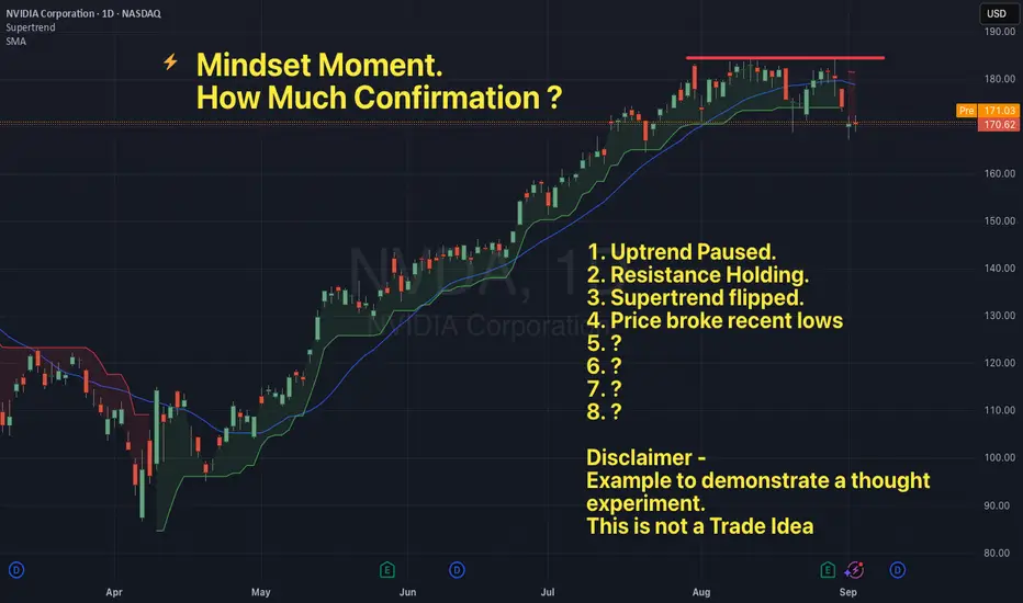
Certainly Uncertain - How Much Confirmation Do You Need?So ... you have what looks like a set up.
"Just one more bar"
"Just wait for the close"
"Wait for this indicator to align"
"Watch for the next to align"
"Ensure this filter shows ‘green lights go’"
But by the time everything lines up
The move has gone.
The horse has bolted
You fumble to enter - all fingers and thumbs
You ‘feel’ like you’re chasing
Perhaps the moment has passed.
Flummoxed - you wonder - what the heck happened here?
Feel familiar?
The search for absolute certainty shows up in subtle ways:
Emotions:
Anxiety builds. A conflict between wanting to act and restraining the impulse. Applying self control with will … but the body and mind unsettled.
Thoughts:
Endless “what if” scenarios.
What if I miss it.
What if it goes without me
What if I just try and get ahead of this at a better price
Physical Cues:
Tension rises in the body showing up as a hand hovering over the mouse, heart rate climbing - eyes fixated on the screens, backside glued to the seat (for fear of missing it).
If you’ve ever experienced this, you may recognise it as feeling cautious or disciplined.
In the pursuit of being disciplined and true to your rules you feel out of alignment and hesitant.
Markets are uncertain by nature.
If we choose to engage with uncertainty, then surely the job is to create a sense of certainty within ourselves.
The question is how do you do this currently?
A coping mechanism that might help:
Breathe.
Centering your breath is one of the most under rated and effective ways to calm ones nervous system.
Reframe your entry as a probability, not a verdict.
Before you click, remind yourself: This trade doesn’t have to be certain, it just has to meet my criteria. Then execute and let the outcome be data - not proof of your worth. Adopt the mantra… ‘ This is one trade in a 1000’
Cultivate the state of certainty in uncertain environments one trade at a time.
From First Trade To Endless Cycle Of Loss (Trading Addiction)Most traders step into the market with a simple thought: “ Just one trade. ”
But when that first small position turns green, the brain celebrates with a rush of dopamine. That sweet moment tricks you into believing you have figured the market out. What feels like confidence is often the first step into a dangerous spiral : the trading addiction cycle.
Hello✌️
Spend 2 minutes ⏰ reading this educational material.
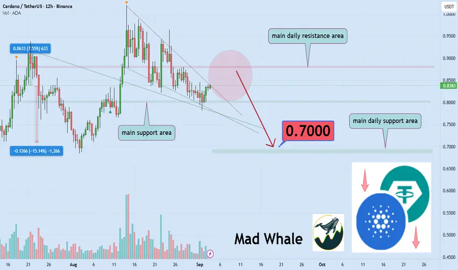
🎯 Analytical Insight on Cardano:
BINANCE:ADAUSDT has lost all key Fibonacci support levels 📉 and is approaching a major daily resistance. If the primary support, clearly marked on the chart, breaks, a drop of at least 15% could follow, targeting around $0.70 ⚠️.
Now , let's dive into the educational section,
🎯 Where It All Begins
It usually starts with harmless intentions like learning, experimenting, or just testing luck. The first quick win feels powerful. The brain records this victory as proof of skill, when in reality it’s often pure randomness. Instead of analyzing why the trade worked, traders rush to repeat the sensation of winning. That’s the invisible first hook.
💡 The Illusion of Small Success
Cognitive bias magnifies those early wins. Traders convince themselves they’ve cracked the code while the truth is they’ve only tasted noise. They stop focusing on analysis and instead chase the feeling. This is how harmless wins plant the seed of reckless entries, random positions, and overconfidence.
🌀 From Wins to Losses
After a few quick wins, overconfidence expands. Position sizes grow. That’s when the market turns. A simple correction wipes out days of profits, triggering the revenge-trading loop. The trader is no longer trading the chart; they’re trading their emotions.
⚠️ The Danger Zone
At this point, discipline disappears. The trader acts like a gambler chasing losses. Risk management is ignored, leverage climbs, and desperation sets in. The spiral accelerates until the account balance is drained.
🧩 The Role of Greed
Greed fuels this engine. After every gain, the brain whispers “more.” After every loss, it screams “get it back now.” That voice is why traders hold too long, re-enter too quickly, and burn capital faster than they ever expect.
🛡 The Real Meaning of Security
Many assume capital security is about wallets or exchanges. In reality, the biggest threat to your money is your own undisciplined mind. Safe investing means protecting yourself from yourself first. Without risk control, even the safest assets vanish.
🔄 The Endless Loop
Every loss tempts another entry. Every failed entry creates the belief “the next one will fix it.” This cycle is how most beginners and even many experienced traders lose their accounts long before they learn discipline.
🧭 The Way Out
Breaking free isn’t about finding a magic indicator or signal. The only way is a structured system, hard rules, and loyalty to them. Discipline is the seatbelt that keeps you alive when the market crashes. Without it, no strategy can save you.
🕹 TradingView Tools Against the Addiction Cycle
This is where TradingView tools can step in like a safeguard.
Alerts: Instead of staring at charts and forcing trades, let alerts call you only when your setups trigger.
Position Size Calculators and custom scripts: They prevent oversized entries that come from emotional overconfidence.
Volume Profile: Reveals zones where serious money moves, giving logic to your trades instead of raw impulse.
Trading Journal on charts: Annotating your own trades makes behavioral mistakes visible, showing you how emotions repeat.
These tools don’t just provide technical data. They create practical boundaries that break emotional patterns before they become addiction.
📌 Three Pieces of Advice to Escape the Trading Addiction Cycle
No profit is worth an undisciplined entry: If your only reason is “it feels right,” that trade is already lost.
Capital is sacred: Protect your principal above all. Profits come and go, but once the core is gone, the game ends.
Discipline beats strategy: The strongest traders are not the smartest, but the most consistent.
✨ Need a little love!
We pour love into every post your support keeps us inspired! 💛 Don’t be shy, we’d love to hear from you on comments. Big thanks , Mad Whale 🐋
📜Please make sure to do your own research before investing, and review the disclaimer provided at the end of each post.
superstition meets charts + free Fibonacci day trading strategymagic arts of finance
The financial markets are often portrayed as cold, logical, and ruthlessly efficient. But let’s be honest sometimes they feel more like a scene out of a fantasy novel than a spreadsheet. Traders have long whispered about strange patterns, uncanny coincidences, and borderline mystical forces shaping price action.
here as some of which i have come across :
🌕 Moon Phases and Market Moves ( sentiment )
It may sound crazy, but research papers and trader folklore alike suggest that full moons and new moons can influence investor sentiment. Some studies claim risk appetite increases around new moons, while full moons see investors turn cautious. Are we ruled by lunar cycles—or are we just night-trading zombies looking for meaning in the stars?
📊 Chart idea: Overlay the S&P 500 or Bitcoin with full moon/new moon markers—watch how eerily often turning points cluster around them.
🍂 The September Effect
Statistically, September has been the worst month for equities for over 100 years. No one knows why maybe it’s tax adjustments, portfolio rebalancing, or just collective fear. Some traders avoid opening new positions in September altogether, calling it the “Market’s Bermuda Triangle.”
chart above shows average monthly returns of U.S stocks and September being the worst performing month..
i recently did a publication on it :
🧙 The Magic of Numbers
Ever heard of the “Rule of 7,” “Golden Ratios,” or Fibonacci retracements? These mystical-sounding formulas often align eerily well with market moves. Whether it’s real order-flow dynamics or just collective belief making it true, traders treat these numbers like sacred spells.
Markets love Fibonacci retracements and extensions. Whether it’s 38.2%, 50%, or 61.8%, prices bounce and stall around these “magic ratios.” Do traders actually create the self-fulfilling prophecy by believing in it? Or is math really the language of the market gods?
on the above chart image of CADCHF, i highlighted the trading day of 03 september 2025 and i took fib retracement from high to low of the day to give following day pivot points or important levels, see how price reacts on the 0.786 or 78.6% making the start of the most significant move for the current day from the fib level and the other notice the reaction on 0.618 or 61.8% is it perfect science or market voodoo?
example 2 :
bitcoin
take the chart above: price climbed, touched the 23.6% retracement (the so-called 0.236 spell), and then began its sharp descent. To the uninitiated, this looks like coincidence. To Fibonacci devotees, it’s evidence that markets bend to the rhythm of sacred ratios.
23.6% → A quick rejection zone, where trend reversals often begin.
38.2% & 50% → Balance points, tested like checkpoints before continuation.
🍀 Lucky & Cursed Superstitions
Some of the strangest trading floor beliefs include:
🔮 The Friday Curse
Many traders avoid holding large positions over the weekend, especially in volatile markets like crypto or FX. The logic: markets can gap when they reopen on Monday due to news or events that happen while markets are closed. Over time, this caution has morphed into a superstition “bad things happen to open trades on Fridays.” Even if nothing mystical is going on, enough people believe it, so Friday liquidity sometimes dries up faster.
🙊 “Never Say Crash”
Similar to how actors won’t say “Macbeth” in a theater, traders avoid saying “crash” out loud, especially in bullish markets. The superstition is that simply naming the disaster can “manifest” it. While rational minds know it’s just psychology, there is a kernel of truth: negative language can amplify fear and spread panic among traders effectively becoming a self-fulfilling prophecy.
🚫 Ticker Taboos
Certain tickers or assets get reputations as cursed—think of infamous stocks that destroyed portfolios (Lehman Brothers in 2008, or meme stocks that wiped out retail traders). Some traders flat-out refuse to touch those names again, no matter how good the setup looks. It’s not unlike avoiding a blackjack table after losing your shirt there once it’s part memory, part superstition.
🧦 Trading Socks & Charms
On trading floors (and now in home offices), you’ll find lucky ties, socks, pens, or even figurines. Traders treat them like talismans to bring good fortune during the session. Statistically, socks don’t move markets but the ritual helps build confidence, and psychology is half the battle in trading. (If you’ve ever put on your “interview shirt” before a big meeting, you understand the vibe.)
🏈 The Super Bowl Indicator
This classic Wall Street superstition claims:
NFC team wins → Stocks rise.
AFC team wins → Stocks fall.
It started because early correlations were spooky-accurate (like 90%+ for several decades). Of course, correlation is not causation, and the pattern eventually broke. Still, it gets dusted off every February as a lighthearted market omen.
☿️ Mercury Retrograde
Astrology believers say Mercury retrograde messes with communication, travel, and technology. In trading, this gets blamed for weird market moves, glitches, or periods of irrational volatility. While pros don’t build strategies around star charts, it highlights an important truth: when markets move strangely and we can’t explain it, humans love to assign cosmic causes.
which superstitions have you heard or come across?
These superstitions blend psychology, history, and trader folklore. Even if they aren’t “real,” they influence behaviour and behaviour is what moves markets.
put together by : Pako Phutietsile as @currencynerd
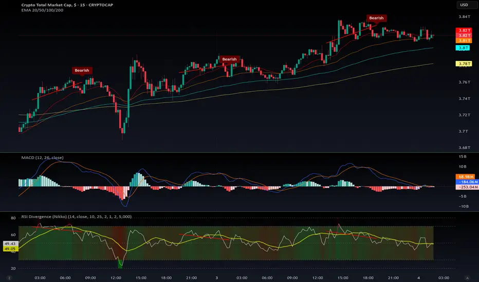
Understanding How Crypto Exchanges Influence Coin PricesUnderstanding How Crypto Exchanges Influence Coin Prices
Cryptocurrency markets often appear unpredictable, with sudden price surges or drops that seem to defy logic. For example, when Bitcoin ( CRYPTOCAP:BTC ) experiences a sharp upward spike—a "green candle"—many altcoins follow almost instantly. Why does this happen so quickly? This tutorial explores the theory that centralized exchanges (e.g., Binance, Coinbase) can manipulate coin prices by adjusting internal database values rather than executing real on-chain trades, and how they may use "pegging ratios" to control price movements of specific coins or ecosystems.
The Myth of Instant Market Reactions
When CRYPTOCAP:BTC surges, altcoins often move in lockstep, seemingly without delay. A common assumption is that millions of investors or market-making bots react simultaneously, causing this synchronized movement. However, natural market reactions typically involve some lag due to order book processing, trader decisions, or bot algorithms. So why is the movement near-instantaneous?
The answer may lie in how centralized exchanges operate. Unlike decentralized exchanges (DEXs), which rely on transparent on-chain transactions, centralized exchanges manage trades internally using their own databases. This means they control virtual coin balances, not necessarily actual blockchain assets. When an exchange wants to "pump" a coin (e.g., increase its price by 10% following a CRYPTOCAP:BTC spike), it doesn't need to buy real coins on the blockchain. Instead, it can simply adjust the coin's value in its database, creating the appearance of market activity without requiring reserve assets.
This internal manipulation allows exchanges to influence prices rapidly, explaining the lack of lag in altcoin movements.
------------------
How Exchanges Peg Coins to Major Assets
Exchanges often peg the price movements of altcoins to major cryptocurrencies like CRYPTOCAP:BTC , CRYPTOCAP:ETH , or CRYPTOCAP:SOL , using a weighted ratio that determines how closely a coin follows these leaders. This pegging isn't a fixed value but a dynamic relationship that can vary by coin or ecosystem. For instance:
Typical Pegging Structure:
50% tied to CRYPTOCAP:BTC (the dominant market driver).
50% tied to other ecosystems (e.g., CRYPTOCAP:ETH for Ethereum-based tokens, CRYPTOCAP:SOL for Solana-based tokens).
Example: A meme coin on the Ethereum blockchain might be pegged 50% to CRYPTOCAP:BTC , 25% to CRYPTOCAP:ETH , and 25% to a general "meme coin" index.
This pegging explains why some coins pump or dump more aggressively than others during market trends. Each coin's price movement is a weighted response to the assets it's tied to.
The Role of Pegging Ratios: Pumps vs. Dumps
Exchanges don't apply uniform ratios for upward and downward price movements. Instead, they may assign positive or negative ratios to influence a coin's trajectory:
Positive Ratio: A coin rises faster than its pegged assets during pumps (upward movements) and falls slower during dumps (downward movements). This increases the coin's value over time, often because the exchange holds a large position and plans to sell later for profit.
Example: CRYPTOCAP:SOL might have a 2:1 positive ratio, rising twice as fast as CRYPTOCAP:BTC during a pump and falling half as fast during a dump.
Other Examples: CRYPTOCAP:BNB (Binance's token) and GETTEX:HYPE often show positive ratios, benefiting from exchange favoritism.
Negative Ratio: A coin rises slower than its pegged assets during pumps and falls faster during dumps. This can gradually erode a coin's value, often used by exchanges to liquidate or delist coins they no longer favor.
Example: SEED_DONKEYDAN_MARKET_CAP:ORDI , pegged to CRYPTOCAP:BTC , may fall faster than CRYPTOCAP:BTC during dumps and rise slower during pumps, leading to a net decline.
Other Examples: CRYPTOCAP:INJ , NYSE:SEI , LSE:TIA often exhibit negative ratios.
Meme coins are a special case, typically pegged to both CRYPTOCAP:BTC and their native blockchain:
CRYPTOCAP:PEPE (Ethereum-based) may have a neutral ratio, moving evenly with CRYPTOCAP:BTC and $ETH.
SEED_DONKEYDAN_MARKET_CAP:BONK (Solana-based) might have a negative ratio, falling faster than CRYPTOCAP:BTC and $SOL.
------------------
Exchange Strategies: Controlling Ecosystems and Liquidation
Exchanges can manipulate entire ecosystems by adjusting ratios for categories of coins. For example:
Setting a 2:1 ratio on all meme coins could make them rise twice as fast as CRYPTOCAP:BTC during a pump, creating hype and attracting retail investors.
Conversely, assigning a negative ratio to an ecosystem (e.g., certain layer-2 tokens) can suppress their value, allowing the exchange to accumulate or liquidate positions.
A notable strategy is slow liquidation:
Exchanges may apply a negative ratio to a coin they wish to delist (e.g., SEED_DONKEYDAN_MARKET_CAP:ORDI ). Over time, the coin's value erodes until it reaches a level where the exchange can justify delisting it, citing "low trading volume" or "lack of interest."
This process creates space for new coins the exchange favors, often ones they hold or have partnerships with.
------------------
Why This Matters for Traders?
The idea that coin prices are driven purely by investor sentiment and organic price action is overly simplistic. Centralized exchanges, with their control over internal databases, can heavily influence price trends. Understanding this can help traders:
Identify Positive-Ratio Coins: These are likely to increase in value over the mid-to-long term. Accumulating coins like CRYPTOCAP:SOL or CRYPTOCAP:BNB during dips could yield profits if their positive ratios persist.
Avoid Negative-Ratio Coins: Coins like SEED_DONKEYDAN_MARKET_CAP:ORDI or CRYPTOCAP:INJ may bleed value over time, draining portfolios unless traded carefully.
Monitor Ecosystem Shifts: Watch for exchange announcements (e.g., new listings, delistings) or unusual price movements that deviate from $BTC/ CRYPTOCAP:ETH trends, as these may signal ratio changes.
------------------
Important Notes
Dynamic Ratios: Pegging ratios are not fixed and can change daily based on exchange strategies, market conditions, or liquidity needs. Always verify current trends with real-time data.
Data Sources: Use tools like CoinGecko, CoinMarketCap, or on-chain analytics (e.g., tradingview) to track correlations between coins and their pegged assets.
Risks of Centralized Exchanges: This tutorial focuses on centralized platforms, not DEXs, where on-chain transparency limits such manipulation. Consider diversifying to DEXs for more predictable trading.
Speculative Nature: While this theory is based on observed market patterns, it remains speculative. Exchanges rarely disclose internal mechanisms, so traders should combine this knowledge with technical analysis and risk management.
------------------
Conclusion
Crypto exchanges wield significant power over coin prices by adjusting virtual balances in their databases and using dynamic pegging ratios. By understanding positive and negative ratios, traders can make informed decisions about which coins to hold or avoid. Always conduct your own research, monitor market trends, and use secure platforms to protect your investments. The crypto market may be rigged in some ways, but knowledge of these mechanics can give you an edge.
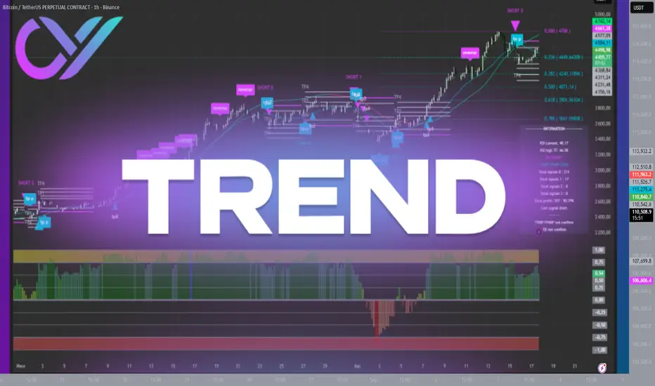
What Is a Trend and How Not to Confuse It With a Correction"One of the first words every trader hears when entering the market is “trend.” It seems simple: a trend is the direction of price movement. But in practice, this is where most mistakes and debates arise. Where is the actual trend, and where is just a correction? What is a reversal, and what is only a pause? Misunderstanding these questions costs money — sometimes an entire account.
Why Is It So Hard to See the Trend?
The challenge lies in the fact that markets always move in waves. Even during a strong uptrend, price will pause, pull back, and create local highs and lows. For a trader, especially a beginner, it’s easy to mistake a correction for a reversal. This often leads to closing trades too early, or holding them too long when it no longer makes sense. Imagine Bitcoin rises from $100,000 to $118,000. Suddenly, price drops to $114,000. Is this the start of a downtrend, or just a pullback before the next push higher? The answer doesn’t lie in emotions but in reading the structure of the trend.
How to Distinguish Trend From Correction
A trend is a sequence of moves where each new impulse confirms the previous one.
- In an uptrend, each new high is higher than the last, and each low also moves higher.
- In a downtrend, each new low drops below the last, and highs remain capped.
A correction, however, is a temporary pullback against the main direction. It doesn’t break the structure. If price in an uptrend pulls back but holds above key support, it’s a correction, not a reversal. Levels and volumes often provide the confirmation. When price tests and holds strong support, the trend stays intact. But if it breaks and consolidates beyond that level, it’s a signal that the market may be reversing.
The Role of Psychology in Mistakes
Most of the time, the problem isn’t theory — it’s psychology. Traders see “collapse” where there is only a normal correction. Or they hope for continuation when the structure is already broken. Greed stops them from taking profit when they should, while fear forces them to close trades at every pullback. Trading then becomes a set of random emotional decisions instead of a structured plan.
What Really Helps
1. Technical analysis. Trendlines, support/resistance, and patterns provide a framework.
2. Multi-timeframe analysis. On lower charts, a correction may look like a full reversal. On higher timeframes, it’s just a pause. You need both perspectives.
3. Algorithmic approach. Automation removes unnecessary emotions. When a system highlights zones, profit levels, and trend shifts, traders can stick to their plan.
4. Staged profit-taking. Even if the market reverses unexpectedly, part of the profit is already secured.
Why This Matters to Every Trader
For beginners, trends and corrections often look identical. Visualization and structure act as a navigator, showing what’s just a pullback and what requires caution — saving years of trial and error.
For intermediate traders, the value is in acceleration. They already know how to read charts but often hesitate in execution. A structured system reduces emotional mistakes and provides clear reference points.
For professionals, the priority is time and discipline. They don’t need definitions of trends — they need a tool that filters out noise, keeps trades consistent, and maximizes holding potential.
For investors, understanding trend vs. correction provides clarity on where to accumulate and where to reduce exposure. It’s not a guessing game but a framework for managing capital.
Final Note
Trend and correction aren’t just textbook terms — they are the foundation of trading. Those who can tell them apart manage trades, instead of being managed by market chaos.
The market will always try to knock you off balance emotionally. But a systematic approach based on technical analysis highlights structure, pinpoints key levels, and removes guesswork. That’s what transforms trading from a lottery into a structured process, where emotions fade and decisions come from cold logic."
Oil Prices & Their Impact on Global MarketsIntroduction
Oil is often called the lifeblood of the global economy. From fueling cars and airplanes to powering industries and generating electricity, oil remains one of the most vital commodities in the modern world. Although renewable energy is growing rapidly, oil still accounts for more than 30% of global energy consumption, making its price movements extremely influential.
When oil prices rise or fall, the impact goes far beyond petrol pumps—it affects inflation, currencies, stock markets, government policies, and even geopolitics. This is why economists, investors, and policymakers closely track crude oil prices.
In this article, we will explore the dynamics of oil pricing, the factors influencing it, and how changes ripple across global markets—touching on inflation, trade balances, stock indices, currency exchange rates, and geopolitical stability.
1. The Role of Oil in the Global Economy
1.1 Oil as a Primary Energy Source
Oil is the backbone of global transportation—cars, trucks, ships, and planes all rely heavily on petroleum.
Petrochemicals derived from oil are used in plastics, fertilizers, medicines, and countless everyday products.
While natural gas and renewables are rising, oil remains indispensable due to its energy density and portability.
1.2 Oil as a Strategic Commodity
Countries treat oil not just as fuel but as a strategic asset.
Nations with large reserves (Saudi Arabia, Russia, Venezuela) hold geopolitical influence.
Import-dependent countries (India, Japan, most of Europe) are vulnerable to supply disruptions.
2. How Oil Prices Are Determined
Oil prices are not set by a single authority but shaped by market forces, geopolitics, and speculation.
2.1 Supply & Demand Dynamics
When demand for oil rises (e.g., during economic booms), prices tend to increase.
Oversupply situations, such as the U.S. shale boom, push prices lower.
2.2 OPEC and OPEC+ Influence
The Organization of the Petroleum Exporting Countries (OPEC), led by Saudi Arabia, plays a major role.
Through coordinated production cuts or increases, OPEC influences global supply.
The OPEC+ alliance (which includes Russia) has further strengthened this control.
2.3 Geopolitical Tensions
Wars, sanctions, and unrest in oil-producing regions can disrupt supply, spiking prices.
Example: The 1973 Arab Oil Embargo caused a fourfold price increase.
Example: Russia–Ukraine war in 2022 pushed oil above $120 per barrel.
2.4 Financial Markets & Speculation
Oil futures traded on exchanges (NYMEX, ICE) allow hedging but also invite speculation.
Hedge funds, institutional investors, and traders amplify price swings.
2.5 Currency Movements
Oil is priced in U.S. dollars, so fluctuations in the dollar’s strength impact oil affordability.
A weaker dollar usually pushes oil prices up, as buyers in other currencies find it cheaper.
3. Historical Oil Price Shocks and Lessons
3.1 The 1973 Oil Crisis
Arab nations cut supply after the Yom Kippur War.
Oil prices quadrupled, triggering stagflation in the West.
3.2 1979 Iranian Revolution
Supply disruptions pushed oil above $100 per barrel (adjusted).
Inflation soared, leading to interest rate hikes.
3.3 1990 Gulf War
Iraqi invasion of Kuwait disrupted supplies.
Prices doubled in a few months.
3.4 2008 Financial Crisis & Oil Spike
Oil hit $147 per barrel in July 2008 before collapsing during the recession.
Showed how closely oil demand ties to economic growth.
3.5 2020 COVID-19 Pandemic
Lockdowns crushed demand; oil futures even went negative (–$37 per barrel) in April 2020.
Highlighted how storage constraints affect pricing.
4. Impact of Oil Prices on Global Markets
Oil price changes create winners and losers depending on whether a country is an importer or exporter.
4.1 Inflation & Consumer Prices
Higher oil prices increase transport and production costs.
This raises food, fuel, and goods prices, contributing to inflation.
Example: In 2022, inflation surged worldwide as oil spiked post-Ukraine war.
4.2 Interest Rates & Monetary Policy
Central banks respond to oil-driven inflation with rate hikes.
Higher interest rates slow growth but stabilize prices.
Example: U.S. Federal Reserve’s aggressive tightening in 2022 was partly due to energy-driven inflation.
4.3 Stock Markets
Rising oil prices benefit energy companies (ExxonMobil, Saudi Aramco).
But they hurt transportation, manufacturing, and consumer sectors.
Oil shocks often trigger volatility in global indices like S&P 500, FTSE, and Nifty.
4.4 Currency Exchange Rates
Oil exporters (Russia, Saudi Arabia, Norway) see their currencies strengthen when oil prices rise.
Importers (India, Turkey, Japan) face currency depreciation due to higher import bills.
4.5 Trade Balances
Import-heavy economies face wider trade deficits during high oil prices.
Exporters accumulate surpluses and build sovereign wealth funds.
Example: Gulf nations reinvest surpluses in global real estate, tech, and financial markets.
4.6 Energy Transition & Renewables
Sustained high oil prices accelerate investments in renewables, EVs, and green hydrogen.
Low oil prices, however, reduce incentives for clean energy adoption.
5. Regional Perspectives
5.1 United States
Once heavily import-dependent, but the shale revolution made it a net exporter.
Rising oil prices benefit U.S. energy companies but hurt consumers.
5.2 Europe
Highly import-dependent, especially on Russia (before 2022).
High prices trigger inflation and energy crises, forcing a faster transition to renewables.
5.3 Middle East
Oil exporters enjoy windfalls during price surges.
However, dependence on oil revenue makes them vulnerable to crashes.
5.4 Asia (India, China, Japan)
Asia is the world’s largest oil consumer.
High prices strain trade balances and weaken currencies.
Example: India’s fiscal deficit widens significantly when oil rises.
5.5 Africa & Latin America
Mixed impact: exporters like Nigeria, Angola, and Venezuela benefit, while importers like South Africa suffer.
6. Oil Prices & Geopolitics
Oil often shapes global power dynamics.
U.S. maintains strong ties with Saudi Arabia due to energy security.
Russia uses oil and gas as geopolitical weapons (e.g., cutting supplies to Europe).
China secures oil through Belt and Road projects and African investments.
Oil-rich countries often gain disproportionate influence in international organizations.
7. Future Outlook: Oil in Transition
7.1 Peak Oil Demand Debate
Some experts predict global oil demand may peak by 2030s due to EVs and clean energy.
Others argue emerging economies will keep demand strong for decades.
7.2 Volatility to Remain
Geopolitics, climate policies, and OPEC actions will ensure continued volatility.
Oil may swing between $60–$120 per barrel frequently.
7.3 Role of Technology
Shale, deep-water drilling, and alternative fuels are reshaping supply.
AI and big data in trading may increase price fluctuations.
7.4 Climate Policies
Carbon taxes, green investments, and net-zero pledges will impact long-term oil demand.
But short-term reliance remains high, keeping oil central to the global economy.
Conclusion
Oil prices act like a thermometer for the global economy. When they rise sharply, inflation, currency weakness, and geopolitical tensions follow. When they crash, exporters struggle, but importers breathe easier. The interconnectedness of oil with financial markets, trade, currencies, and politics makes it one of the most powerful forces shaping our world.
As the world transitions toward renewable energy, oil will eventually lose its dominance—but for at least the next two decades, its price swings will remain a critical driver of global economic stability and instability.
The Four Different Sideways TrendsIn the modern Market Structure, stocks, indexes and industry indexes move sideways or trend moving horizontally most of the time. Understanding this phenomenon and how to use it to your advantage is important to learn.
There are 4 different types of price moving sideways:
1. The consolidation is a very narrow price range, often less than 5% but can be wider. The consolidation trend usually lasts a few days to a few weeks. The price action is very tight and small. Pro traders dominate consolidations usually. Price pings between a narrow price range low and high. Price is a penny spread or few pennies at most. This means the candlesticks are very very small and tightly compacted.
Consolidations are relatively easy to identify on a stock chart. These pattern create a liquidity shift which an HFT AI algo discovers and triggers its automated orders to drive price up or down based on the positions the pro traders are holding.
Consolidations create fast paced momentum and velocity runs that you can take advantage of IF you learn to enter the position BEFORE HFTs and then the smaller funds, retail day traders and gamblers drive price upward. You and pro traders ride the run until you see a Pro trader exit candle pattern to close the position.
2. The Platform Position sideways trend is also very precise with consistent highs and lows. These are the realm of the Dark Pools hidden accumulation and if you are trying to day trade a platform then it will whipsaw and cause losses. The width is too narrow for day trading. The platform is about 10% of the price in width. Platforms form after a market has had a correction and numerous stocks are building bottoms. Once the bottom completes and the Dark Pools recognize that the stock price is below fundamental levels the Dark Pool raise their buy zone price range to a new level. Often HFTs gap up a stock and then Dark Pools resume their hidden accumulation at that higher level. The goal is to enter just before the HFT gap up to the new fundamental level for swing or day trading.
Platforms offer low risk and the position can be held for weeks or months generating excellent income with minimal time for busy trades who do not have the time to swing trade. Platforms are also good for swing traders if they time their entry correctly.
3. Sideways trends are a mix of retail investors and retail day traders, smaller funds managers and sometimes Dark Pools hidden within the wider sideways trend. These trends with the wider mix of market participants have inconsistent highs and lows which often times causes retail day traders losses as they do not understand the dynamics of the wide sideways trend. These sideways trends are more than 10% and as wide as 20% of the stock price.
4. The Trading Range is the hardest to trade and often causes the most losses as frequently the trading range is so wide it is not easily recognized on the daily charts but is visible and obvious on a weekly chart. The inconsistent highs and lows within the very wide trading range cause problems and losses for most day and swing retail traders.
The size differential of each sideways trend tells you WHO is in control of price and how to trade it for maximum profits, lower risk, and to make trading fun rather than harder.

ESG Investing in Global MarketsChapter 1: Understanding ESG Investing
1.1 Definition of ESG
Environmental (E): Concerns around climate change, carbon emissions, renewable energy adoption, water usage, biodiversity, pollution control, and sustainable resource management.
Social (S): Focuses on human rights, labor practices, workplace diversity, employee well-being, community engagement, customer protection, and social equity.
Governance (G): Relates to corporate governance structures, board independence, executive pay, transparency, ethics, shareholder rights, and anti-corruption measures.
Together, these dimensions create a holistic lens for evaluating companies beyond financial metrics, helping investors identify long-term risks and opportunities.
1.2 Evolution of ESG
1960s-1970s: Emergence of ethical investing linked to religious and social movements, e.g., opposition to apartheid or tobacco.
1990s: Rise of Socially Responsible Investing (SRI), focusing on excluding “sin stocks” (alcohol, gambling, weapons).
2000s: The United Nations launched the Principles for Responsible Investment (PRI) in 2006, formally embedding ESG into mainstream finance.
2010s onwards: ESG investing surged amid global concerns over climate change, social inequality, and corporate scandals.
1.3 Why ESG Matters
Risk Management: Companies ignoring ESG risks (e.g., climate lawsuits, governance failures) face financial penalties.
Long-Term Returns: Studies show firms with strong ESG practices often outperform peers over the long run.
Investor Demand: Millennials and Gen Z increasingly prefer ESG-aligned investments.
Regulatory Push: Governments worldwide are mandating ESG disclosures and carbon neutrality goals.
Chapter 2: ESG Investing Strategies
Investors adopt multiple approaches to integrate ESG factors:
Negative/Exclusionary Screening – Avoiding industries such as tobacco, coal, or controversial weapons.
Positive/Best-in-Class Screening – Selecting companies with superior ESG scores relative to peers.
Thematic Investing – Focusing on ESG themes like renewable energy, clean water, or gender diversity.
Impact Investing – Investing to generate measurable social and environmental outcomes alongside returns.
Active Ownership/Stewardship – Using shareholder influence to push for ESG improvements in companies.
ESG Integration – Embedding ESG considerations directly into financial analysis and valuation.
Chapter 3: ESG in Global Markets
3.1 North America
The U.S. has seen rapid growth in ESG funds, though political debates around ESG (especially in energy-heavy states) have created polarization.
Major asset managers like BlackRock, Vanguard, and State Street integrate ESG into products.
Regulatory frameworks (SEC climate disclosure proposals) are shaping ESG reporting.
3.2 Europe
Europe leads globally in ESG adoption, with strong regulatory support such as the EU Sustainable Finance Disclosure Regulation (SFDR) and the EU Taxonomy.
Scandinavian countries (Norway, Sweden, Denmark) are pioneers in sustainable finance, often divesting from fossil fuels.
ESG ETFs and green bonds dominate European sustainable investment flows.
3.3 Asia-Pacific
Japan’s Government Pension Investment Fund (GPIF), one of the world’s largest, actively invests in ESG indices.
China is promoting green finance under its carbon neutrality by 2060 pledge, but faces challenges in standardization and transparency.
India is witnessing growth in ESG mutual funds, driven by SEBI (Securities and Exchange Board of India) regulations and corporate sustainability goals.
3.4 Emerging Markets
ESG in emerging markets is growing but uneven.
Investors face challenges such as limited disclosure, weaker governance, and political risks.
Nonetheless, ESG adoption is rising in markets like Brazil (Amazon deforestation issues), South Africa, and Southeast Asia.
Chapter 4: ESG Performance and Market Impact
4.1 Financial Returns
Research indicates ESG funds often perform competitively with, or even outperform, traditional funds. Key findings include:
ESG funds are more resilient during downturns (e.g., COVID-19 crisis).
Companies with high ESG ratings often enjoy lower cost of capital.
4.2 Green Bonds and Sustainable Finance
Green Bonds have grown into a $2 trillion+ market globally, financing renewable energy, clean transport, and sustainable infrastructure.
Other innovations include sustainability-linked loans and social bonds.
4.3 Corporate Transformation
ESG pressure has driven oil majors (e.g., Shell, BP) to diversify into renewables.
Tech firms (e.g., Apple, Microsoft) are committing to carbon neutrality.
Banks and insurers are phasing out financing for coal projects.
Chapter 5: Challenges in ESG Investing
Despite growth, ESG investing faces several obstacles:
Lack of Standardization: Different ESG rating agencies use varied methodologies, creating inconsistency.
Greenwashing: Some firms exaggerate ESG credentials to attract investors without real impact.
Data Gaps: In emerging markets, ESG disclosures are limited or unreliable.
Short-Termism: Many investors still prioritize quarterly returns over long-term ESG impact.
Political Backlash: ESG has become politicized, particularly in the U.S., leading to regulatory tensions.
Chapter 6: Case Studies
6.1 Tesla – A Controversial ESG Icon
Tesla is often seen as a leader in clean technology due to its role in electric mobility. However, concerns about labor practices, governance issues, and supply chain risks (e.g., cobalt mining) complicate its ESG profile.
6.2 BP & Energy Transition
After the 2010 Deepwater Horizon disaster, BP rebranded itself as a greener energy company, investing heavily in renewables. This illustrates how ESG pressure can push legacy firms toward transformation.
6.3 Unilever – Social & Environmental Responsibility
Unilever integrates ESG principles deeply into its operations, focusing on sustainable sourcing, waste reduction, and social equity, earning strong support from ESG investors.
Chapter 7: Regulatory and Institutional Landscape
UN PRI: Global standard promoting ESG integration.
TCFD (Task Force on Climate-Related Financial Disclosures): Encourages climate risk reporting.
IFRS & ISSB (International Sustainability Standards Board): Working on global ESG reporting frameworks.
National Regulations:
U.S. SEC climate disclosures.
EU SFDR & EU Taxonomy.
India’s Business Responsibility and Sustainability Report (BRSR).
Chapter 8: Future of ESG Investing
The future of ESG investing is shaped by megatrends:
Climate Transition: Net-zero commitments will drive massive capital flows into clean energy, green tech, and sustainable infrastructure.
Technology & Data: AI, big data, and blockchain will improve ESG measurement, reducing greenwashing.
Retail Investor Growth: ESG-focused ETFs and robo-advisors will make sustainable investing more accessible.
Integration with Corporate Strategy: ESG will move from a reporting exercise to a core business strategy.
Emerging Market Potential: Growth in Asia, Africa, and Latin America will define the next wave of ESG capital allocation.
Conclusion
ESG investing is no longer an optional strategy—it is becoming a main pillar of global finance. Investors, regulators, and corporations recognize that long-term economic prosperity is inseparable from sustainability, social responsibility, and sound governance. While challenges such as greenwashing, inconsistent standards, and political backlash persist, the momentum is undeniable.
As global challenges like climate change, inequality, and governance scandals intensify, ESG investing provides a roadmap for channeling capital toward solutions that create sustainable financial returns and a better world. In the next decade, ESG will not just influence markets—it will define them.

Energy Transition & Commodity MarketsSection 1: Understanding the Energy Transition
1.1 Definition
Energy transition is the process of moving from an energy system dominated by fossil fuels to one that relies on low-carbon and renewable energy sources. Unlike past energy transitions (from wood to coal in the Industrial Revolution, or from coal to oil in the 20th century), today’s transition is policy-driven and environmentally motivated, with the goal of achieving net zero carbon emissions by mid-century.
1.2 Drivers of Energy Transition
Climate Change Mitigation: To limit global warming to 1.5–2°C, greenhouse gas emissions must be drastically reduced.
Technological Innovation: Falling costs of solar, wind, batteries, and green hydrogen are accelerating adoption.
Energy Security: Dependence on imported fossil fuels creates vulnerabilities; renewables offer greater resilience.
Investor & Consumer Demand: ESG (Environmental, Social, and Governance) investing and rising public awareness are pushing corporations to decarbonize.
1.3 Key Pillars
Electrification of transport and industry
Renewable energy deployment
Energy efficiency improvements
Carbon capture and storage (CCS)
Hydrogen economy development
Section 2: Commodity Markets – An Overview
Commodity markets are broadly divided into:
Energy Commodities – oil, natural gas, coal.
Metals & Minerals – iron ore, copper, aluminum, lithium, cobalt, nickel, rare earths.
Agricultural Commodities – grains, oilseeds, sugar, biofuels (ethanol, biodiesel).
Commodity markets are crucial because they:
Provide raw materials for energy systems.
Influence inflation, currency stability, and trade balances.
Reflect global supply-demand dynamics and geopolitical risks.
As energy transition reshapes global energy flows, commodity markets are entering a new cycle of volatility, opportunities, and risks.
Section 3: Fossil Fuels in Transition
3.1 Oil
Oil has been the dominant energy commodity for decades, but demand growth is slowing.
Short-term Outlook: Oil remains essential for transportation, petrochemicals, and aviation.
Long-term Outlook: EV adoption, efficiency improvements, and policies to phase out ICE (internal combustion engine) vehicles could lead to peak oil demand by 2030–2040.
Impact: Oil-exporting countries may face revenue shocks, while diversification becomes urgent.
3.2 Natural Gas
Often seen as a “bridge fuel”, natural gas emits less CO₂ than coal and oil.
Role in Transition: Supports grid stability as renewables expand; key in hydrogen production (blue hydrogen).
Risks: Methane leakage undermines its climate benefits; long-term role uncertain.
3.3 Coal
Coal is the biggest loser in the energy transition.
Decline: Many advanced economies are phasing out coal due to high carbon intensity.
Exceptions: Some Asian countries still rely on coal for cheap electricity.
Impact: Coal markets are shrinking; future limited to metallurgical coal for steelmaking.
Section 4: Green Metals and Minerals
The clean energy revolution is metal-intensive. According to the International Energy Agency (IEA), a typical EV requires 6 times more minerals than a conventional car, while a wind farm needs 9 times more mineral resources than a gas-fired plant.
4.1 Copper
Used in wiring, EV motors, and renewable energy grids.
Copper demand expected to double by 2040.
4.2 Lithium
Key for lithium-ion batteries in EVs and storage.
Demand projected to increase over 40 times by 2040.
4.3 Cobalt
Critical in high-density batteries.
Supply concentrated in the Democratic Republic of Congo (DRC), raising geopolitical and ethical concerns.
4.4 Nickel
Important for battery cathodes.
Growing demand in EV sector; Indonesia emerging as a dominant supplier.
4.5 Rare Earth Elements (REEs)
Essential for wind turbines, EV motors, and defense technologies.
Supply dominated by China, creating potential geopolitical risks.
Section 5: Renewable Energy & Commodity Linkages
5.1 Solar Power
Relies heavily on silicon, silver, aluminum, and glass.
Commodity markets for silver are increasingly influenced by solar demand.
5.2 Wind Energy
Requires large amounts of steel, copper, and rare earths.
Offshore wind is even more metal-intensive than onshore.
5.3 Hydrogen Economy
Green hydrogen needs renewable electricity and electrolyzers (requiring platinum, iridium).
Blue hydrogen depends on natural gas and carbon capture.
5.4 Energy Storage
Batteries are the backbone of renewables integration.
Metals like lithium, cobalt, nickel, and graphite see exponential demand.
Section 6: Geopolitical and Economic Dimensions
6.1 Resource Nationalism
As green commodities rise in importance, countries rich in lithium, cobalt, and rare earths may adopt resource nationalism policies, similar to OPEC’s oil strategies.
6.2 Supply Chain Vulnerabilities
Concentration of rare earth supply in China.
Lithium reserves in South America’s “Lithium Triangle” (Argentina, Bolivia, Chile).
Cobalt dominated by DRC, raising human rights concerns.
6.3 Trade Wars & Strategic Competition
U.S. and Europe are investing in domestic critical mineral supply chains to reduce dependency.
Strategic competition may reshape global trade patterns.
Section 7: Financial Markets and Investment Trends
7.1 ESG Investing
Investors are shifting capital towards green energy and sustainable commodities.
Oil and coal financing becoming harder to secure.
7.2 Carbon Markets
Carbon pricing and emissions trading systems (ETS) affect fossil fuel demand.
Commodities linked to higher carbon footprints face declining attractiveness.
7.3 Commodity Price Volatility
Green transition is creating supercycles in certain metals.
Shortages may push prices higher, while substitution and recycling could stabilize markets.
Section 8: Challenges in the Energy Transition
8.1 Supply Constraints
Mining and refining capacity may lag demand.
Long lead times (10–15 years) for new mines.
8.2 Environmental & Social Risks
Mining expansion may harm ecosystems and local communities.
Human rights abuses in supply chains (child labor in cobalt mining).
8.3 Technology Uncertainty
Battery chemistry may shift, reducing reliance on certain metals.
Hydrogen adoption uncertain due to costs and infrastructure needs.
8.4 Policy Uncertainty
Inconsistent climate policies create market volatility.
Subsidy cuts or political shifts can slow adoption.
Section 9: Opportunities in the Transition
9.1 Green Commodity Supercycle
Metals like lithium, copper, and nickel could see decades of sustained demand growth.
9.2 Recycling and Circular Economy
Battery recycling could reduce dependence on virgin mining.
“Urban mining” of e-waste emerging as a new industry.
9.3 Technological Innovation
Advances in battery tech (solid-state batteries).
Substitutes for scarce materials (cobalt-free batteries).
9.4 Emerging Markets Growth
Developing countries rich in green resources may benefit from foreign investment.
Section 10: Future Outlook
The energy transition will not be linear; it will involve disruptions, volatility, and regional variations. However, the direction is clear:
Fossil fuels will gradually decline.
Metals and minerals critical to clean energy will dominate commodity markets.
Policies and geopolitics will heavily influence market outcomes.
By 2050, the global energy system could look dramatically different—one where electricity is the main energy vector, renewables provide the majority of supply, and commodity markets revolve around green resources rather than hydrocarbons.
Conclusion
The energy transition is reshaping the foundations of the global commodity markets. While fossil fuels are gradually losing ground, metals and minerals essential to renewable technologies are entering a period of unprecedented demand growth. This shift brings both challenges—such as supply constraints, geopolitical risks, and environmental concerns—and opportunities, including green investment booms, technological innovation, and sustainable growth.
Ultimately, the interplay between energy transition and commodity markets will define the economic and geopolitical landscape of the 21st century. Countries, companies, and investors that adapt swiftly will be the leaders of the new energy age, while those clinging to the old fossil-fuel paradigm risk being left behind.

Do Chart Patterns in Forex really Work?If you’ve been trading for a while, you’ve probably seen them: Head & Shoulders, Double Tops, Flags, Pennants, Wedges, Triangles.
They’re plastered across textbooks, YouTube tutorials, and trading courses as if they’re the secret key to unlocking market profits.
But let’s be brutally honest for a second…
Do these chart patterns actually work in Forex, or are we just drawing shapes on random price moves and calling it “analysis”?
This question has divided traders for decades. Some swear by chart patterns and build entire systems around them. Others call them illusions that only look good in hindsight. Let’s dig deeper.
Why Traders Believe in Chart Patterns
They Represent Market Psychology
A chart pattern isn’t just lines, it’s a visual story of buyer vs. seller psychology.
A Double Top represents a strong rejection of higher prices and often signals a potential reversal from bullish to bearish.
A Flag after a strong move shows a pause (profit-taking) before continuation.
These patterns give structure to the chaos of price action.
Risk-to-Reward Framework
Patterns give traders a ready-made blueprint for entries, stop losses, and targets.
For example, a triangle breakout trader knows exactly where the invalidation point is (back inside the triangle) and where the profit projection could be (measured move).
Self-Fulfilling Prophecy
This is perhaps the strongest argument. Because thousands of traders around the world believe in these patterns, they act on them and their collective actions make the patterns play out.
Why Chart Patterns Fail (Especially in Forex)
Subjectivity
A “perfect” pattern doesn’t exist.
What looks like a clean Double Top to one trader may look like noise to another.
Beginners often force patterns into charts that aren’t really there.
The lack of consistency is a big problem.
False Breakouts
Forex is notorious for liquidity hunts. Institutions know where breakout traders place their stops, and often price will fake out of a pattern before reversing.
Many traders lose money not because patterns don’t work, but because they take the first breakout without waiting for confirmation.
Lack of Statistical Evidence
Several academic studies and even backtests on historical data have shown mixed results.
Some patterns (like Flags) have slightly better-than-random odds.
Others (like Triangles) often fail as much as they succeed.
Without confluence, relying on patterns alone is like flipping a coin.
My Take, The Truth About Patterns
Patterns are not signals. They are frameworks for context.
Here’s the formula I believe in:
➡️ Pattern + Market Context + Confluence + Risk Management = Edge
Pattern: The shape itself (e.g., Head & Shoulders).
Market Context: Where it forms matters more than the pattern itself. Is it at a key supply/demand zone? Is it against the trend?
Confluence: Combine with liquidity, imbalances, order blocks, volume, or fundamentals.
Risk Management: Even the best setup fails sometimes. Stop losses and position sizing keep you in the game.
Trading patterns blindly is gambling.
Trading patterns with context and discipline is strategy.
Something Most Traders Don’t Realize
Patterns don’t predict the market, they reveal behaviour.
Think of them like a language of crowd psychology:
A Wedge isn’t predicting a breakout. It’s showing momentum is slowing and a big move is likely to come.
A Double Top isn’t magical, it’s just showing price struggled twice at the same resistance level.
A Flag doesn’t guarantee continuation, it simply shows a healthy pause in trend momentum.
The power comes from interpreting what the market is saying through the pattern, not from memorizing shapes like flashcards.
Discussion for the Community
This is where I’d love to hear from you:
Do YOU trade chart patterns?
If yes, which ones do you find most reliable in Forex?
Do you think patterns are useful, or are they overrated relics from the past?
Do you believe they’re “real” or just a self-fulfilling prophecy because enough traders act on them?
Bonus question: Have you ever backtested patterns systematically and what did you find?
📌 My goal here is to start an honest, evidence-based conversation about chart patterns. The more perspectives, the better so don’t hold back in the comments.
If you found this useful, hit that boost icon and thank you!
Bottom line:
Chart patterns are neither a scam nor a holy grail. They are tools and like any tool, their effectiveness depends on the skill of the trader using them.
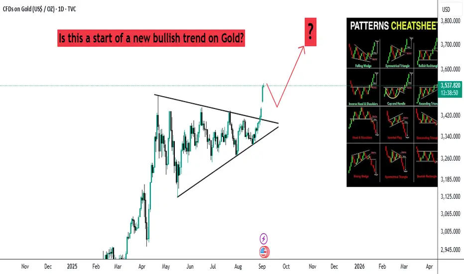
Trade idea update on GBPUSDMarket has been choppy but that’s the importance of a good SL placement. The good position we placed our SL helped us survive the noise in the market till Tp


Bullish Gartley and ABCD Equality in DXYBullish Gartley and ABCD Equality in DXY.. What are your thoughts on DXY bottoming out ?

Exchange Rate Dynamics & FluctuationsPart 1: What Are Exchange Rates?
An exchange rate is essentially the price of one currency in terms of another. For example:
Direct quote: 1 USD = 83 INR → How many rupees per dollar.
Indirect quote: 1 INR = 0.012 USD → How many dollars per rupee.
Functions of Exchange Rates
Facilitate international trade – exporters and importers settle payments.
Enable cross-border investment – FDI, FIIs, bonds, equity markets.
Act as indicators of competitiveness – strong vs weak currency matters for exports.
Transmit global shocks – inflation, oil prices, interest rate changes often flow through currency movements.
Part 2: Exchange Rate Systems
Countries adopt different systems to manage their currencies:
Fixed Exchange Rate System
Currency pegged to gold or another currency (e.g., Bretton Woods system).
Provides stability but reduces flexibility.
Floating Exchange Rate System
Currency value determined purely by demand and supply in forex markets.
More volatile but allows automatic adjustment.
Managed Floating (Dirty Float)
Combination of both: central banks intervene occasionally to prevent extreme volatility.
Example: India’s rupee is a managed float.
Currency Pegs & Boards
Some countries peg their currencies to the US dollar or euro (e.g., Hong Kong dollar).
Offers stability but imports inflation/monetary policy from the anchor country.
Part 3: Theories of Exchange Rate Determination
Economists have proposed several models to explain exchange rate movements:
Purchasing Power Parity (PPP)
Currencies adjust to equalize the purchasing power of different countries.
Example: If a burger costs $5 in the US and ₹400 in India, then PPP exchange rate = 400/5 = 80.
Interest Rate Parity (IRP)
Interest rate differences between countries affect forward exchange rates.
Higher interest rates attract capital inflows, strengthening the currency.
Balance of Payments Approach
Exchange rate depends on trade balance (exports-imports) and capital flows.
Trade surplus strengthens currency; deficit weakens it.
Monetary Approach
Currency value linked to money supply and inflation.
Higher inflation depreciates a currency.
Asset Market Approach
Exchange rate determined by demand and supply of financial assets across countries.
Part 4: Key Drivers of Exchange Rate Fluctuations
1. Demand and Supply of Currencies
Like any commodity, exchange rates are influenced by demand and supply. If more people want dollars (for oil imports, for example), the dollar strengthens.
2. Interest Rates
High domestic interest rates attract foreign capital → appreciation of the local currency.
Low interest rates cause outflows → depreciation.
3. Inflation Rates
Countries with lower inflation rates tend to see currency appreciation, as purchasing power is preserved.
4. Trade Balance
Export surplus → stronger currency.
Import-heavy economy → weaker currency.
5. Foreign Direct Investment (FDI) and Portfolio Flows
When investors buy stocks, bonds, or companies in a country, they demand that country’s currency → appreciation.
6. Speculation and Market Sentiment
Traders often buy or sell currencies based on expectations. If markets expect the rupee to fall, speculative selling accelerates the decline.
7. Central Bank Intervention
Central banks sometimes buy/sell foreign currencies to stabilize their domestic currency.
Example: RBI selling dollars to support the rupee.
8. Geopolitical Events and Political Stability
Wars, elections, coups, and policy changes can trigger sharp movements.
9. Commodity Prices
Oil-exporting nations’ currencies (like Russia’s ruble) rise when oil prices rise.
Oil-importing countries (like India) see their currency weaken when oil becomes expensive.
10. Global Risk Appetite
During crises, investors flock to “safe haven” currencies (USD, CHF, JPY), causing them to appreciate.
Part 5: Types of Exchange Rate Fluctuations
Appreciation – Currency value rises (e.g., USD/INR falls from 83 → 80).
Depreciation – Currency value falls (e.g., USD/INR rises from 83 → 86).
Devaluation – Government/central bank officially reduces the currency’s value under fixed system.
Revaluation – Official increase in value.
Volatility – Short-term fluctuations due to speculative trading, news, or shocks.
Part 6: Real-World Examples
Asian Financial Crisis (1997)
Thai baht collapse spread across Asia.
Triggered by excessive borrowing and weak reserves.
Eurozone Debt Crisis (2010–12)
Euro weakened due to fears of Greek and other sovereign defaults.
COVID-19 Pandemic (2020)
Investors rushed into the dollar as a safe haven.
Emerging market currencies depreciated sharply.
Russia-Ukraine War (2022)
Ruble crashed initially, then recovered after capital controls and oil exports.
Indian Rupee Movements
1991 crisis forced devaluation.
2008 crisis → rupee fell due to capital outflows.
Recent years: rupee under pressure due to oil imports and strong US dollar.
Part 7: Implications of Exchange Rate Fluctuations
1. On Trade
A weaker currency makes exports cheaper, boosting demand abroad.
But it makes imports more expensive, adding inflationary pressure.
2. On Inflation
Import-dependent economies (like India with oil) see higher inflation when their currency depreciates.
3. On Investment
FIIs gain/loss depends on both stock performance and currency movement.
Currency depreciation can wipe out returns.
4. On Government Policy
Central banks adjust interest rates, intervene in forex markets, and build reserves.
5. On Common People
Travelers, students abroad, NRIs, and businesses all feel the effect of currency changes.
Part 8: Managing Exchange Rate Risk
Hedging with Derivatives
Forwards, futures, options, and swaps help companies lock in exchange rates.
Natural Hedging
Matching foreign currency revenues with expenses.
Diversification
Spreading trade and investments across multiple currencies.
Government Policies
Building forex reserves, imposing capital controls, or adjusting interest rates.
Part 9: The Future of Exchange Rate Dynamics
Digital Currencies
Central Bank Digital Currencies (CBDCs) may change cross-border payments.
Geopolitical Realignment
De-dollarization attempts by BRICS could alter forex dynamics.
Climate & Commodity Shocks
Weather events affecting agriculture and energy may impact currencies.
AI & Algorithmic Trading
High-frequency forex trading will increase volatility.
Conclusion
Exchange rate dynamics and fluctuations are at the heart of the global economy. They result from a complex interplay of trade, investment, inflation, interest rates, speculation, and geopolitics. No single factor explains all movements—currencies reflect the combined pulse of global markets.
For policymakers, managing exchange rates is a balancing act between stability and flexibility. For businesses, it’s a constant risk to hedge against. For investors, it’s both a challenge and an opportunity.
Ultimately, exchange rates are more than numbers—they represent the relative strength, stability, and future expectations of nations in the interconnected global system.
Currency Pegs & Managed Exchange Rates1. Theoretical Background: Exchange Rate Systems
Before diving into pegs and managed exchange rates, it is essential to understand the spectrum of exchange rate arrangements.
Free-floating exchange rates
Determined entirely by supply and demand in the foreign exchange market.
No direct government or central bank intervention.
Example: U.S. dollar, Japanese yen, British pound.
Fixed exchange rates
Currency value is tied to another currency or a basket of currencies.
Requires constant intervention to maintain the fixed rate.
Example: Gold standard (historical), Hong Kong dollar peg to USD.
Intermediate systems
Includes currency pegs, crawling pegs, and managed floats.
Aim to combine stability with some degree of flexibility.
Most countries today operate in this middle ground.
Thus, currency pegs and managed exchange rates fall under the "intermediate" category—neither fully rigid nor fully market-determined.
2. Currency Pegs: Definition and Mechanism
A currency peg (also called a fixed exchange rate) is when a country’s central bank commits to maintaining its currency at a specific exchange rate relative to another major currency or basket.
How It Works:
The central bank monitors the foreign exchange market.
If the domestic currency depreciates below the peg, the central bank intervenes by selling foreign reserves (usually U.S. dollars or euros) and buying domestic currency to restore the peg.
If the domestic currency appreciates above the peg, the central bank buys foreign currency and sells domestic currency.
Maintaining the peg requires large reserves of foreign currency and tight monetary discipline.
Types of Pegs:
Hard Pegs
Currency is immovably fixed, sometimes legally.
Example: Currency board systems like in Hong Kong.
Soft Pegs
Fixed within a narrow band but adjustable under certain conditions.
Example: China before 2005 pegged the yuan to the U.S. dollar but adjusted occasionally.
Crawling Pegs
The peg is adjusted gradually, often in response to inflation or trade deficits.
Example: Several Latin American countries have used crawling pegs.
Historical Context
The most famous peg system was the Bretton Woods system (1944–1971), where most currencies were pegged to the U.S. dollar, which in turn was pegged to gold at $35 per ounce. This system collapsed when the U.S. could no longer maintain gold convertibility, leading to today’s diverse exchange rate regimes.
3. Managed Exchange Rates: Definition and Mechanism
A managed exchange rate (or dirty float) is a system where a currency is allowed to fluctuate according to market forces but with periodic government or central bank interventions.
Key Characteristics:
The exchange rate is not strictly fixed.
Central banks intervene to prevent excessive volatility or maintain competitiveness.
Intervention tools include:
Buying/selling foreign currency.
Adjusting interest rates.
Using capital controls.
Example:
China’s managed float system since 2005. The yuan is not entirely free-floating; the People’s Bank of China (PBoC) sets a daily reference rate and allows limited fluctuations within a band.
Why Managed Floats?
To avoid the instability of free-floating currencies.
To retain flexibility in adjusting to shocks.
To prevent speculative attacks common under rigid pegs.
4. Advantages of Currency Pegs
Stability in Trade & Investment
Pegs reduce exchange rate risk, encouraging foreign trade and investment.
Example: Hong Kong’s USD peg has attracted global businesses.
Inflation Control
Pegging to a stable currency can help reduce inflation in countries with weak monetary institutions.
Credibility for Developing Economies
Pegs provide a clear and transparent exchange rate target, increasing investor confidence.
Tourism & Remittances
Stable exchange rates benefit countries reliant on tourism and remittance inflows.
5. Disadvantages of Currency Pegs
Loss of Monetary Policy Independence
Central banks cannot freely adjust interest rates.
Domestic priorities like unemployment may be ignored.
Vulnerability to Speculative Attacks
If investors doubt the peg’s sustainability, massive speculative outflows can trigger a crisis.
Example: 1997 Asian Financial Crisis.
Requirement of Large Foreign Reserves
Maintaining a peg requires holding vast reserves, which is costly.
Importing Inflation/Deflation
Pegging to another currency means importing that country’s monetary policy.
6. Advantages of Managed Exchange Rates
Flexibility with Stability
Combines market-driven efficiency with government’s ability to smooth volatility.
Crisis Management Tool
Central banks can intervene during crises to stabilize the currency.
Helps Maintain Competitiveness
Countries can prevent their currencies from appreciating too much, supporting exports.
Avoids Extreme Currency Misalignments
Intervention reduces excessive swings caused by speculation or capital flows.
7. Disadvantages of Managed Exchange Rates
Uncertainty & Lack of Transparency
Since interventions are unpredictable, investors may face uncertainty.
Cost of Intervention
Frequent interventions require reserves and may distort the market.
Moral Hazard
Businesses may rely on government protection against currency fluctuations instead of proper risk management.
Political Manipulation
Governments may artificially keep currencies undervalued, leading to trade disputes.
Example: Accusations against China for "currency manipulation."
8. Case Studies
Case Study 1: Hong Kong Dollar Peg
Since 1983, pegged at HK$7.8 per USD.
Helped maintain Hong Kong as a financial hub.
However, limits monetary independence, especially during crises.
Case Study 2: Chinese Yuan (RMB)
Pre-2005: Strict peg to USD.
Post-2005: Managed float with a daily reference rate.
This allowed China to gradually internationalize the yuan and maintain export competitiveness.
Case Study 3: Argentina’s Currency Board (1991–2001)
Peso pegged 1:1 to USD to fight hyperinflation.
Initially successful, but eventually collapsed due to loss of competitiveness and inability to devalue.
Led to a severe financial crisis.
Case Study 4: Asian Financial Crisis (1997–98)
Many Southeast Asian economies had soft pegs to the dollar.
When investors lost confidence, speculative attacks forced massive devaluations.
Highlights the vulnerability of rigid or semi-rigid pegs without sufficient reserves.
9. Role of IMF and International Community
The IMF monitors exchange rate policies and provides support during crises.
It offers countries advice on choosing appropriate regimes depending on their structure.
For developing nations, IMF often recommends flexible systems to absorb shocks.
However, IMF-supported stabilization programs sometimes push countries toward pegs for credibility.
10. Modern Challenges
Globalization & Capital Mobility
Rapid capital flows make it harder to defend pegs.
Currency Wars
Countries may manipulate exchange rates for trade advantage, creating global tensions.
Dollar Dominance
Since many pegs are tied to the U.S. dollar, shifts in U.S. monetary policy have global spillovers.
Digital Currencies & Fintech
Central bank digital currencies (CBDCs) may transform exchange rate management in the future.
Conclusion
Currency pegs and managed exchange rate regimes are essential tools in global financial architecture. Pegs provide stability but sacrifice flexibility, often leading to crises if mismanaged. Managed exchange rates offer a middle path—allowing currencies to respond to market forces while enabling governments to intervene when necessary.
The choice of regime depends on a country’s economic structure, trade composition, inflation history, and policy credibility. There is no one-size-fits-all approach. For small, open economies reliant on trade, pegs can be beneficial. For larger, emerging markets, managed floats may provide the necessary balance. Ultimately, successful exchange rate management requires strong institutions, prudent policies, and adaptability in a constantly evolving global economy.

Currency Wars & Competitive Devaluation1. Understanding Currency Wars
1.1 Definition
A currency war refers to a situation in which countries intentionally manipulate their exchange rates to gain trade advantages. This is usually done by keeping their currency undervalued against major global currencies (such as the US Dollar or Euro), making their exports cheaper and imports more expensive.
1.2 Difference between Normal Exchange Rate Policies and Currency Wars
Normal Exchange Rate Adjustments: Countries may let market forces or monetary policy determine currency values based on economic fundamentals.
Currency Wars: Deliberate interventions—such as excessive printing of money, cutting interest rates aggressively, or directly buying foreign currencies—to weaken domestic currency beyond fundamentals.
1.3 Why Nations Engage in Currency Wars
Boost Exports: Cheaper currency makes exports more competitive.
Reduce Imports: Costlier imports encourage domestic consumption.
Stimulate Growth: Export-led growth can help recover from recessions.
Tackle Deflation: Weak currency raises import prices, generating inflation.
2. Competitive Devaluation
2.1 Definition
Competitive devaluation occurs when multiple countries sequentially lower the value of their currencies in response to each other’s actions. It’s essentially a “race to the bottom,” where no one wins in the long run, but everyone suffers from instability.
2.2 Mechanisms of Devaluation
Monetary Policy Tools: Central banks reduce interest rates or engage in quantitative easing (printing money).
Foreign Exchange Interventions: Governments or central banks sell domestic currency and buy foreign reserves.
Capital Controls: Restrictions on inflows/outflows to maintain currency depreciation.
2.3 Historical Perspective of Competitive Devaluation
1930s Great Depression: Countries abandoned the gold standard and devalued currencies to boost exports.
1970s Bretton Woods Collapse: Exchange rate system breakdown triggered currency adjustments.
2008 Financial Crisis Aftermath: The US, Japan, and emerging economies engaged in aggressive monetary easing.
3. Historical Episodes of Currency Wars
3.1 The Great Depression (1930s)
Many countries abandoned the gold standard to devalue their currencies.
The US devalued the dollar under Roosevelt, while the UK left the gold standard in 1931.
This created a spiral of competitive devaluations, worsening global economic tensions.
3.2 Bretton Woods System Collapse (1971)
After World War II, the Bretton Woods system pegged currencies to the US dollar.
In 1971, the Nixon Shock ended dollar-gold convertibility.
Currencies began floating, leading to sharp adjustments and devaluations.
3.3 Plaza Accord (1985)
The US dollar had appreciated significantly, hurting American exports.
G5 nations (US, Japan, UK, France, West Germany) agreed to weaken the dollar.
A coordinated effort prevented disorderly currency competition.
3.4 Post-2008 Financial Crisis
The US Federal Reserve launched quantitative easing (QE), weakening the dollar.
Emerging markets like Brazil accused the US of starting a “currency war.”
Japan’s Abenomics policy in 2012–13 was also criticized as competitive devaluation.
4. Tools and Strategies of Currency Wars
4.1 Monetary Policy Tools
Lowering Interest Rates: Reduces returns for investors, weakening currency.
Quantitative Easing (QE): Increases money supply, pressuring currency downward.
4.2 Direct Interventions
Central banks buy foreign currencies (e.g., US dollars, euros) to push domestic currency lower.
Example: China’s PBoC interventions to keep the yuan undervalued.
4.3 Trade and Fiscal Measures
Export subsidies or import tariffs indirectly support devaluation effects.
Capital controls prevent appreciation from foreign investment inflows.
4.4 Communication & Market Signals
Central banks sometimes issue statements signaling dovish policies to influence expectations.
5. Impact of Currency Wars
5.1 Positive Effects (Short-Term)
Boosts Exports: Domestic products become cheaper abroad.
Supports Growth: Export-led demand revives economies.
Manages Deflation: Import inflation helps economies facing deflation.
5.2 Negative Effects (Long-Term)
Retaliation: Other countries devalue, nullifying initial benefits.
Inflationary Pressure: Rising import prices fuel inflation.
Loss of Investor Confidence: Sudden devaluations deter foreign investors.
Trade Tensions: Devaluation leads to accusations of currency manipulation.
Global Instability: Competitive devaluation creates uncertainty in capital flows.
6. Case Studies of Currency Wars
6.1 The US and China
The US has long accused China of keeping the yuan undervalued.
This helped China’s export-led growth model, but created global imbalances.
The 2019 US-China trade war also had a currency dimension, with the yuan weakening.
6.2 Japan’s Abenomics (2012–2013)
Japan used aggressive monetary easing to weaken the yen.
This helped Japanese exports but attracted criticism from trading partners.
6.3 Emerging Market Economies
Countries like Brazil, India, and South Korea faced currency inflows due to US QE.
To protect domestic industries, they intervened to curb currency appreciation.
7. Role of International Institutions
7.1 International Monetary Fund (IMF)
Monitors exchange rate policies.
Can label a country a “currency manipulator” if it deliberately undervalues its currency.
Provides a platform for coordination to avoid competitive devaluations.
7.2 G20 and G7
Forums where countries pledge to avoid competitive devaluation.
Example: G20 statement in 2013 against currency wars.
8. Theoretical Perspectives
8.1 Beggar-Thy-Neighbor Policy
Currency wars are a form of “beggar-thy-neighbor” policy—where one nation’s gain (through exports) comes at another’s expense.
8.2 Game Theory and Currency Wars
Each country has an incentive to devalue, but if all devalue, everyone loses.
This creates a prisoner’s dilemma in international economics.
9. Currency Wars in the 21st Century
9.1 Digital Currencies and Devaluation
Central Bank Digital Currencies (CBDCs) could alter how nations influence exchange rates.
Competition among digital currencies may add new layers to currency wars.
9.2 Geopolitics and Sanctions
The US dollar’s dominance gives the US leverage through sanctions.
Countries like Russia and China promote alternatives (yuan, ruble, gold).
9.3 Post-COVID Era
Pandemic recovery led to massive stimulus and QE across the world.
The risk of currency tensions resurfaced as nations pursued divergent recovery paths.
10. Preventing Currency Wars
10.1 Coordination through Global Forums
Stronger cooperation at IMF, G20, WTO levels can reduce unilateral actions.
10.2 Transparent Monetary Policies
Clear communication by central banks helps avoid misinterpretation of currency intentions.
10.3 Diversified Global Reserve System
Reducing dependence on the US dollar could limit imbalances.
10.4 Regional Currency Agreements
Like the Eurozone, regional cooperation may prevent internal currency competition.
Conclusion
Currency wars and competitive devaluation are complex phenomena that reveal the deep interconnectedness of global economies. While weakening a currency may bring short-term benefits in terms of exports and growth, the long-term consequences often outweigh the advantages. Retaliatory actions, inflationary pressures, trade tensions, and financial instability make currency wars a dangerous economic strategy.
In today’s globalized world, where supply chains and financial markets are deeply integrated, no country can devalue its way to prosperity without harming others. The challenge, therefore, lies in balancing domestic economic needs with global stability. International cooperation, transparency in monetary policies, and reforms in global financial governance remain essential to preventing destructive cycles of competitive devaluation.
Currency wars are, in essence, economic battles without winners. History shows us that the path of cooperation, not confrontation, leads to sustainable prosperity.
Impact of Currency Fluctuations on Global TradeIntroduction
Global trade is the lifeline of the modern economy. It connects countries, industries, and consumers across borders, enabling the exchange of goods, services, capital, and technology. However, at the core of every international transaction lies a critical factor that often gets overlooked in public discussions—currency exchange rates.
Currency fluctuations—the rise and fall of the value of one currency relative to another—play a significant role in shaping trade flows, competitiveness, profitability, and even the stability of entire economies. Exchange rate volatility can determine whether exports are competitive in global markets, how much importers pay for foreign goods, and how investors allocate capital across nations.
This essay explores the impact of currency fluctuations on global trade, breaking down causes, mechanisms, case studies, and long-term implications. It also looks at how governments, central banks, corporations, and financial institutions respond to mitigate risks associated with exchange rate volatility.
Understanding Currency Fluctuations
Currency fluctuations occur when the value of one currency rises or falls relative to another. The foreign exchange (forex) market, the largest financial market in the world, facilitates the buying and selling of currencies. Exchange rates are influenced by supply and demand, interest rates, inflation, political stability, monetary policy, and market speculation.
For example, if the Indian Rupee (INR) weakens against the US Dollar (USD), then Indian exporters receive more rupees for each dollar earned, making exports more competitive. On the other hand, importers must pay more for foreign goods priced in dollars, making imports costlier.
Key terms:
Appreciation: When a currency strengthens relative to another.
Depreciation: When a currency weakens relative to another.
Volatility: The degree of variation in currency values over time.
Causes of Currency Fluctuations
Monetary Policy & Interest Rates
Central banks influence exchange rates through interest rate decisions. Higher interest rates attract foreign capital, strengthening the currency, while lower rates weaken it.
Inflation Levels
Countries with lower inflation typically see currency appreciation, as purchasing power is preserved. High inflation erodes value.
Trade Balances
Nations running trade surpluses (exports > imports) often see stronger currencies, while deficits weaken them.
Capital Flows & Foreign Investment
Strong inflows of foreign direct investment (FDI) or portfolio investment increase demand for a currency, boosting its value.
Political & Economic Stability
Stable countries attract investors, strengthening their currency, while instability leads to capital flight and depreciation.
Market Speculation
Traders in the forex market bet on future movements, sometimes amplifying volatility.
Mechanisms of Impact on Global Trade
1. Export Competitiveness
When a country’s currency depreciates, its exports become cheaper for foreign buyers, boosting demand.
When a currency appreciates, exports become expensive, reducing competitiveness.
2. Import Costs
Currency depreciation increases the cost of imported raw materials, fuel, and machinery.
Appreciation makes imports cheaper, lowering input costs for domestic industries.
3. Profit Margins of Businesses
Exporters benefit from weaker domestic currencies, while import-heavy industries suffer.
Multinational corporations with global operations must manage “translation risk” when consolidating earnings from various currencies.
4. Balance of Payments (BoP)
Persistent depreciation can reduce trade deficits by discouraging imports and encouraging exports.
However, volatility creates uncertainty that disrupts long-term trade agreements.
5. Consumer Prices & Inflation
Currency depreciation makes imports costlier, leading to inflationary pressures in domestic markets.
This reduces consumer purchasing power and alters consumption patterns.
Case Studies: Real-World Examples
1. The US Dollar and Global Trade
The US dollar is the world’s reserve currency, used in most international trade. When the dollar strengthens:
Emerging markets struggle, as their imports become costlier.
US exporters lose competitiveness abroad.
Oil and commodity prices (often denominated in USD) rise for other countries.
2. Japan’s Yen Depreciation (2012–2015)
Japan deliberately weakened its yen under “Abenomics” to boost exports.
Japanese automakers and electronics manufacturers benefited.
Import costs for energy and food rose, impacting consumers.
3. Indian Rupee Volatility
The INR often faces depreciation pressures due to oil imports and trade deficits.
Exporters in IT and textiles gain from weaker rupee.
Oil importers, airlines, and electronics manufacturers face higher costs.
4. Eurozone Crises (2010–2012)
During the sovereign debt crisis, euro depreciation initially supported European exports. However, uncertainty discouraged investment and hurt overall trade confidence.
5. Chinese Yuan Management
China manages its currency to remain competitive in global trade. A weaker yuan supports Chinese exports, though it has often drawn criticism from trading partners accusing China of “currency manipulation.”
Short-Term vs Long-Term Impacts
Short-Term Effects:
Exporters and importers immediately feel gains or losses from currency shifts.
Volatility disrupts pricing strategies, contracts, and supply chains.
Long-Term Effects:
Persistent depreciation can erode investor confidence, discouraging capital inflows.
Companies may relocate production to hedge against currency risks.
Exchange rate instability may encourage protectionism and tariffs.
Sector-Wise Impact
Energy Sector
Oil prices, usually denominated in USD, fluctuate with dollar strength. Importing nations face inflation when their currency weakens.
Technology & Services
Outsourcing destinations like India benefit when their currency weakens, as dollar earnings translate into higher domestic revenue.
Manufacturing & Automobiles
Export-oriented industries gain from weaker home currencies. However, dependency on imported raw materials can offset benefits.
Agriculture & Commodities
Farmers in export-driven economies gain from weaker currencies. But fertilizer, equipment, and fuel imports become costlier.
Tools to Manage Currency Risks
1. Hedging Instruments
Forward Contracts: Lock in exchange rates for future transactions.
Options: Provide flexibility to buy/sell at a fixed rate.
Swaps: Exchange currency cash flows between parties.
2. Diversification
Multinationals diversify production and sourcing across countries to reduce exposure.
3. Central Bank Intervention
Central banks buy/sell currencies to stabilize volatility.
4. Trade Agreements
Regional trade blocs (e.g., EU, ASEAN) reduce intra-region currency risk by using common or pegged currencies.
Winners and Losers in Currency Fluctuations
Winners: Exporters during depreciation, importers during appreciation, forex traders exploiting volatility.
Losers: Import-dependent industries during depreciation, debt-heavy countries with foreign loans, consumers facing inflation.
Broader Economic Implications
Global Supply Chains
Exchange rate volatility complicates cost management in multinational supply chains.
Foreign Debt Servicing
Countries with debt denominated in foreign currencies face higher repayment costs if their currency depreciates.
Trade Wars & Protectionism
Currency disputes can lead to accusations of manipulation, tariffs, and retaliatory trade measures.
Financial Market Volatility
Sudden currency swings trigger capital outflows from emerging markets, destabilizing stock and bond markets.
Future Outlook
Digital Currencies & CBDCs: The rise of central bank digital currencies could reduce transaction costs and lower forex volatility.
Regionalization of Trade: More trade within blocs may reduce exposure to dollar dominance.
Greater Use of Hedging Tools: Firms will increasingly rely on sophisticated financial instruments to manage risk.
Geopolitical Uncertainty: Wars, sanctions, and supply chain disruptions will continue to drive currency volatility.
Conclusion
Currency fluctuations are both an opportunity and a risk in global trade. While depreciation can stimulate exports, it also raises import costs and inflation. Appreciation makes imports cheaper but hurts exporters. The net effect depends on a nation’s trade structure, economic resilience, and ability to manage risks.
For businesses, managing currency risk is now as important as managing production or marketing. Governments must balance exchange rate stability with economic growth, while central banks act as guardians against excessive volatility.
In an interconnected world, no nation is immune from the impact of currency swings. Exchange rate management and risk mitigation strategies will remain central to ensuring global trade continues to thrive despite fluctuations.