Rectified BB% for option tradingThis indicator shows the bollinger bands against the price all expressed in percentage of the mean BB value. With one sight you can see the amplitude of BB and the variation of the price, evaluate a reenter of the price in the BB.
The relative price is visualized as a candle with open/high/low/close value exspressed as percentage deviation from the BB mean
The indicator include a modified RSI, remapped from 0/100 to -100/100.
You can choose the BB parameters (length, standard deviation multiplier) and the RSI parameter (length, overbougth threshold, ovrsold threshold)
You can exclude/include the candles and the RSI line.
The indicator can be used to sell options when the volatility is high (the bollinger band is wide) and the price is reentering inside the bands.
If the price is forming a supply or demand area it can be a good opportunity to sell a bull put or a bear call
The RSI can be used as confirm of the supply/demand formation
If the bollinger band is narrow and the RSI is overbought/oversold it indicate a better opportunity to buy options
the indicator is designed to work with daily timeframe and default parameters.
Impliedvolatility

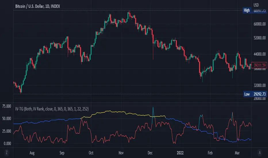
Implied Volatility Suite (TG Fork)Displays the Implied Volatility, which is usually calculated from options, but here is calculated indirectly from spot price directly, either using a model or model-free using the VIXfix.
The model-free VIXfix based approach can detect times of high volatility, which usually coincides with panic and hence lowest prices. Inversely, the model-based approach can detect times of highest greed.
Forked and updated by Tartigradia to fix some issues in the calculations, convert to pinescript v5 and reverse engineered to reproduce the "Implied Volatility Rank & Model Free IVR" indicator by the same author (but closed source) and allow to plot both model-based and model-free implied volatilities simultaneously.
If you like this indicator, please show the original author SegaRKO some love:
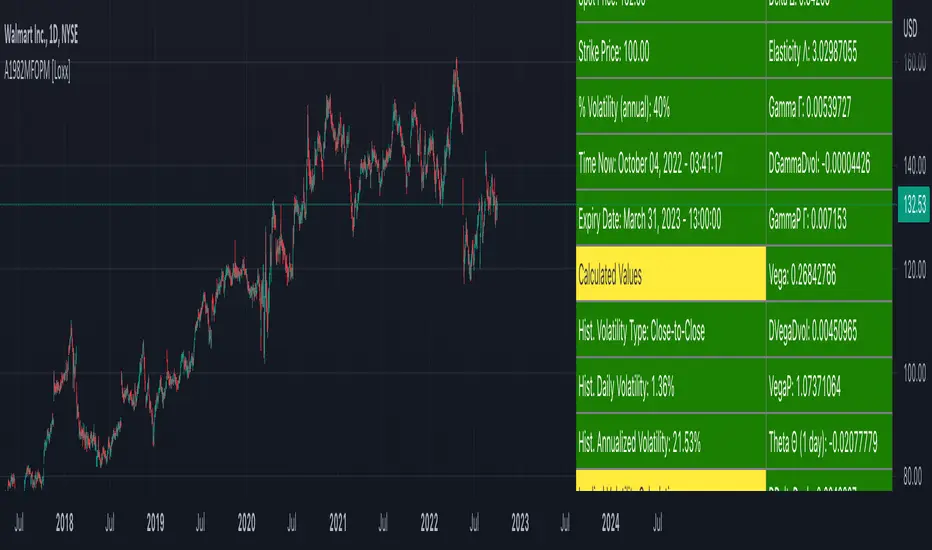
Asay (1982) Margined Futures Option Pricing Model [Loxx]Asay (1982) Margined Futures Option Pricing Model is an adaptation of the Black-Scholes-Merton Option Pricing Model including Analytical Greeks and implied volatility calculations. The following information is an excerpt from Espen Gaarder Haug's book "Option Pricing Formulas". This version is to price Options on Futures where premium is fully margined. This means the Risk-free Rate, dividend, and cost to carry are all zero. The options sensitivities (Greeks) are the partial derivatives of the Black-Scholes-Merton ( BSM ) formula. Analytical Greeks for our purposes here are broken down into various categories:
Delta Greeks: Delta, DDeltaDvol, Elasticity
Gamma Greeks: Gamma, GammaP, DGammaDvol, Speed
Vega Greeks: Vega , DVegaDvol/Vomma, VegaP
Theta Greeks: Theta
Probability Greeks: StrikeDelta, Risk Neutral Density
(See the code for more details)
Black-Scholes-Merton Option Pricing
The Black-Scholes-Merton model can be "generalized" by incorporating a cost-of-carry rate b. This model can be used to price European options on stocks, stocks paying a continuous dividend yield, options on futures , and currency options:
c = S * e^((b - r) * T) * N(d1) - X * e^(-r * T) * N(d2)
p = X * e^(-r * T) * N(-d2) - S * e^((b - r) * T) * N(-d1)
where
d1 = (log(S / X) + (b + v^2 / 2) * T) / (v * T^0.5)
d2 = d1 - v * T^0.5
b = r ... gives the Black and Scholes (1973) stock option model.
b = r — q ... gives the Merton (1973) stock option model with continuous dividend yield q.
b = 0 ... gives the Black (1976) futures option model.
b = 0 and r = 0 ... gives the Asay (1982) margined futures option model. <== this is the one used for this indicator!
b = r — rf ... gives the Garman and Kohlhagen (1983) currency option model.
Inputs
S = Stock price.
X = Strike price of option.
T = Time to expiration in years.
r = Risk-free rate
d = dividend yield
v = Volatility of the underlying asset price
cnd (x) = The cumulative normal distribution function
nd(x) = The standard normal density function
convertingToCCRate(r, cmp ) = Rate compounder
gImpliedVolatilityNR(string CallPutFlag, float S, float x, float T, float r, float b, float cm , float epsilon) = Implied volatility via Newton Raphson
gBlackScholesImpVolBisection(string CallPutFlag, float S, float x, float T, float r, float b, float cm ) = implied volatility via bisection
Implied Volatility: The Bisection Method
The Newton-Raphson method requires knowledge of the partial derivative of the option pricing formula with respect to volatility ( vega ) when searching for the implied volatility . For some options (exotic and American options in particular), vega is not known analytically. The bisection method is an even simpler method to estimate implied volatility when vega is unknown. The bisection method requires two initial volatility estimates (seed values):
1. A "low" estimate of the implied volatility , al, corresponding to an option value, CL
2. A "high" volatility estimate, aH, corresponding to an option value, CH
The option market price, Cm , lies between CL and cH . The bisection estimate is given as the linear interpolation between the two estimates:
v(i + 1) = v(L) + (c(m) - c(L)) * (v(H) - v(L)) / (c(H) - c(L))
Replace v(L) with v(i + 1) if c(v(i + 1)) < c(m), or else replace v(H) with v(i + 1) if c(v(i + 1)) > c(m) until |c(m) - c(v(i + 1))| <= E, at which point v(i + 1) is the implied volatility and E is the desired degree of accuracy.
Implied Volatility: Newton-Raphson Method
The Newton-Raphson method is an efficient way to find the implied volatility of an option contract. It is nothing more than a simple iteration technique for solving one-dimensional nonlinear equations (any introductory textbook in calculus will offer an intuitive explanation). The method seldom uses more than two to three iterations before it converges to the implied volatility . Let
v(i + 1) = v(i) + (c(v(i)) - c(m)) / (dc / dv (i))
until |c(m) - c(v(i + 1))| <= E at which point v(i + 1) is the implied volatility , E is the desired degree of accuracy, c(m) is the market price of the option, and dc/ dv (i) is the vega of the option evaluaated at v(i) (the sensitivity of the option value for a small change in volatility ).
Things to know
Only works on the daily timeframe and for the current source price.
You can adjust the text size to fit the screen
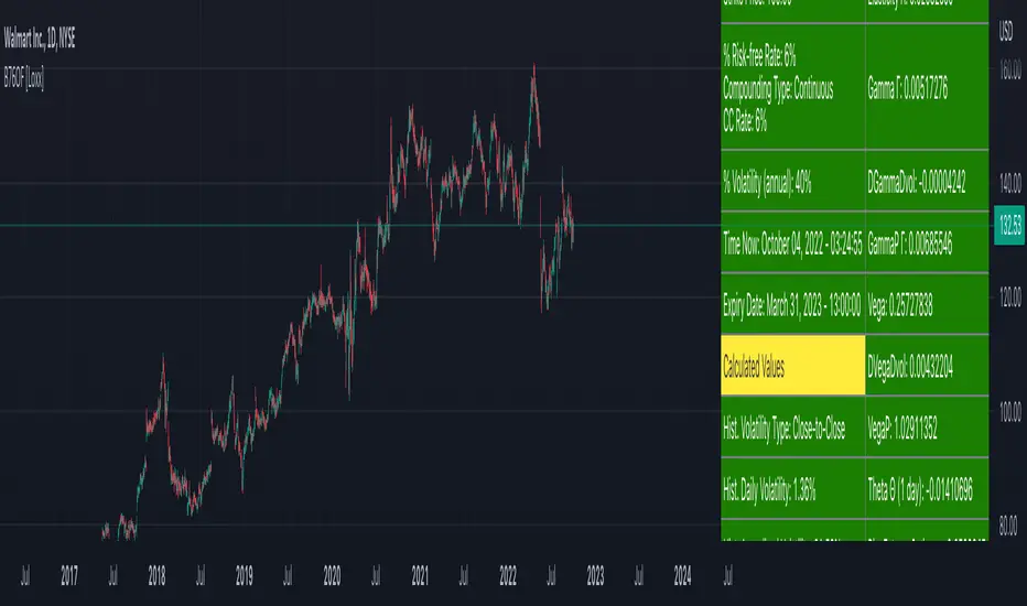
Black-76 Options on Futures [Loxx]Black-76 Options on Futures is an adaptation of the Black-Scholes-Merton Option Pricing Model including Analytical Greeks and implied volatility calculations. The following information is an excerpt from Espen Gaarder Haug's book "Option Pricing Formulas". This version is to price Options on Futures. The options sensitivities (Greeks) are the partial derivatives of the Black-Scholes-Merton ( BSM ) formula. Analytical Greeks for our purposes here are broken down into various categories:
Delta Greeks: Delta, DDeltaDvol, Elasticity
Gamma Greeks: Gamma, GammaP, DGammaDvol, Speed
Vega Greeks: Vega , DVegaDvol/Vomma, VegaP
Theta Greeks: Theta
Rate/Carry Greeks: Rho futures option
Probability Greeks: StrikeDelta, Risk Neutral Density
(See the code for more details)
Black-Scholes-Merton Option Pricing
The Black-Scholes-Merton model can be "generalized" by incorporating a cost-of-carry rate b. This model can be used to price European options on stocks, stocks paying a continuous dividend yield, options on futures , and currency options:
c = S * e^((b - r) * T) * N(d1) - X * e^(-r * T) * N(d2)
p = X * e^(-r * T) * N(-d2) - S * e^((b - r) * T) * N(-d1)
where
d1 = (log(S / X) + (b + v^2 / 2) * T) / (v * T^0.5)
d2 = d1 - v * T^0.5
b = r ... gives the Black and Scholes (1973) stock option model.
b = r — q ... gives the Merton (1973) stock option model with continuous dividend yield q.
b = 0 ... gives the Black (1976) futures option model. <== this is the one used for this indicator!
b = 0 and r = 0 ... gives the Asay (1982) margined futures option model.
b = r — rf ... gives the Garman and Kohlhagen (1983) currency option model.
Inputs
S = Stock price.
X = Strike price of option.
T = Time to expiration in years.
r = Risk-free rate
d = dividend yield
v = Volatility of the underlying asset price
cnd (x) = The cumulative normal distribution function
nd(x) = The standard normal density function
convertingToCCRate(r, cmp ) = Rate compounder
gImpliedVolatilityNR(string CallPutFlag, float S, float x, float T, float r, float b, float cm , float epsilon) = Implied volatility via Newton Raphson
gBlackScholesImpVolBisection(string CallPutFlag, float S, float x, float T, float r, float b, float cm ) = implied volatility via bisection
Implied Volatility: The Bisection Method
The Newton-Raphson method requires knowledge of the partial derivative of the option pricing formula with respect to volatility ( vega ) when searching for the implied volatility . For some options (exotic and American options in particular), vega is not known analytically. The bisection method is an even simpler method to estimate implied volatility when vega is unknown. The bisection method requires two initial volatility estimates (seed values):
1. A "low" estimate of the implied volatility , al, corresponding to an option value, CL
2. A "high" volatility estimate, aH, corresponding to an option value, CH
The option market price, Cm , lies between CL and cH . The bisection estimate is given as the linear interpolation between the two estimates:
v(i + 1) = v(L) + (c(m) - c(L)) * (v(H) - v(L)) / (c(H) - c(L))
Replace v(L) with v(i + 1) if c(v(i + 1)) < c(m), or else replace v(H) with v(i + 1) if c(v(i + 1)) > c(m) until |c(m) - c(v(i + 1))| <= E, at which point v(i + 1) is the implied volatility and E is the desired degree of accuracy.
Implied Volatility: Newton-Raphson Method
The Newton-Raphson method is an efficient way to find the implied volatility of an option contract. It is nothing more than a simple iteration technique for solving one-dimensional nonlinear equations (any introductory textbook in calculus will offer an intuitive explanation). The method seldom uses more than two to three iterations before it converges to the implied volatility . Let
v(i + 1) = v(i) + (c(v(i)) - c(m)) / (dc / dv (i))
until |c(m) - c(v(i + 1))| <= E at which point v(i + 1) is the implied volatility , E is the desired degree of accuracy, c(m) is the market price of the option, and dc/ dv (i) is the vega of the option evaluaated at v(i) (the sensitivity of the option value for a small change in volatility ).
Things to know
Only works on the daily timeframe and for the current source price.
You can adjust the text size to fit the screen
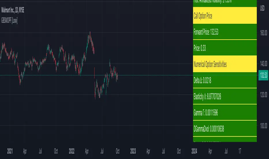
Garman and Kohlhagen (1983) for Currency Options [Loxx]Garman and Kohlhagen (1983) for Currency Options is an adaptation of the Black-Scholes-Merton Option Pricing Model including Analytical Greeks and implied volatility calculations. The following information is an excerpt from Espen Gaarder Haug's book "Option Pricing Formulas". This version of BSMOPM is to price Currency Options. The options sensitivities (Greeks) are the partial derivatives of the Black-Scholes-Merton ( BSM ) formula. Analytical Greeks for our purposes here are broken down into various categories:
Delta Greeks: Delta, DDeltaDvol, Elasticity
Gamma Greeks: Gamma, GammaP, DGammaDSpot/speed, DGammaDvol/Zomma
Vega Greeks: Vega , DVegaDvol/Vomma, VegaP, Speed
Theta Greeks: Theta
Rate/Carry Greeks: Rho, Rho futures option, Carry Rho, Phi/Rho2
Probability Greeks: StrikeDelta, Risk Neutral Density
(See the code for more details)
Black-Scholes-Merton Option Pricing for Currency Options
The Garman and Kohlhagen (1983) modified Black-Scholes model can be used to price European currency options; see also Grabbe (1983). The model is mathematically equivalent to the Merton (1973) model presented earlier. The only difference is that the dividend yield is replaced by the risk-free rate of the foreign currency rf:
c = S * e^(-rf * T) * N(d1) - X * e^(-r * T) * N(d2)
p = X * e^(-r * T) * N(-d2) - S * e^(-rf * T) * N(-d1)
where
d1 = (log(S / X) + (r - rf + v^2 / 2) * T) / (v * T^0.5)
d2 = d1 - v * T^0.5
For more information on currency options, see DeRosa (2000)
Inputs
S = Stock price.
X = Strike price of option.
T = Time to expiration in years.
r = Risk-free rate
rf = Risk-free rate of the foreign currency
v = Volatility of the underlying asset price
cnd (x) = The cumulative normal distribution function
nd(x) = The standard normal density function
convertingToCCRate(r, cmp ) = Rate compounder
gImpliedVolatilityNR(string CallPutFlag, float S, float x, float T, float r, float b, float cm , float epsilon) = Implied volatility via Newton Raphson
gBlackScholesImpVolBisection(string CallPutFlag, float S, float x, float T, float r, float b, float cm ) = implied volatility via bisection
Implied Volatility: The Bisection Method
The Newton-Raphson method requires knowledge of the partial derivative of the option pricing formula with respect to volatility ( vega ) when searching for the implied volatility . For some options (exotic and American options in particular), vega is not known analytically. The bisection method is an even simpler method to estimate implied volatility when vega is unknown. The bisection method requires two initial volatility estimates (seed values):
1. A "low" estimate of the implied volatility , al, corresponding to an option value, CL
2. A "high" volatility estimate, aH, corresponding to an option value, CH
The option market price, Cm , lies between CL and cH . The bisection estimate is given as the linear interpolation between the two estimates:
v(i + 1) = v(L) + (c(m) - c(L)) * (v(H) - v(L)) / (c(H) - c(L))
Replace v(L) with v(i + 1) if c(v(i + 1)) < c(m), or else replace v(H) with v(i + 1) if c(v(i + 1)) > c(m) until |c(m) - c(v(i + 1))| <= E, at which point v(i + 1) is the implied volatility and E is the desired degree of accuracy.
Implied Volatility: Newton-Raphson Method
The Newton-Raphson method is an efficient way to find the implied volatility of an option contract. It is nothing more than a simple iteration technique for solving one-dimensional nonlinear equations (any introductory textbook in calculus will offer an intuitive explanation). The method seldom uses more than two to three iterations before it converges to the implied volatility . Let
v(i + 1) = v(i) + (c(v(i)) - c(m)) / (dc / dv (i))
until |c(m) - c(v(i + 1))| <= E at which point v(i + 1) is the implied volatility , E is the desired degree of accuracy, c(m) is the market price of the option, and dc/ dv (i) is the vega of the option evaluaated at v(i) (the sensitivity of the option value for a small change in volatility ).
Things to know
Only works on the daily timeframe and for the current source price.
You can adjust the text size to fit the screen
Related indicators:
BSM OPM 1973 w/ Continuous Dividend Yield
Black-Scholes 1973 OPM on Non-Dividend Paying Stocks
Generalized Black-Scholes-Merton w/ Analytical Greeks
Generalized Black-Scholes-Merton Option Pricing Formula
Sprenkle 1964 Option Pricing Model w/ Num. Greeks
Modified Bachelier Option Pricing Model w/ Num. Greeks
Bachelier 1900 Option Pricing Model w/ Numerical Greeks

Black-Scholes 1973 OPM on Non-Dividend Paying Stocks [Loxx]Black-Scholes 1973 OPM on Non-Dividend Paying Stocks is an adaptation of the Black-Scholes-Merton Option Pricing Model including Analytical Greeks and implied volatility calculations. Making b equal to r yields the BSM model where dividends are not considered. The following information is an excerpt from Espen Gaarder Haug's book "Option Pricing Formulas". The options sensitivities (Greeks) are the partial derivatives of the Black-Scholes-Merton ( BSM ) formula. For our purposes here are, Analytical Greeks are broken down into various categories:
Delta Greeks: Delta, DDeltaDvol, Elasticity
Gamma Greeks: Gamma, GammaP, DGammaDSpot/speed, DGammaDvol/Zomma
Vega Greeks: Vega , DVegaDvol/Vomma, VegaP
Theta Greeks: Theta
Rate/Carry Greeks: Rho
Probability Greeks: StrikeDelta, Risk Neutral Density
(See the code for more details)
Black-Scholes-Merton Option Pricing
The BSM formula and its binomial counterpart may easily be the most used "probability model/tool" in everyday use — even if we con- sider all other scientific disciplines. Literally tens of thousands of people, including traders, market makers, and salespeople, use option formulas several times a day. Hardly any other area has seen such dramatic growth as the options and derivatives businesses. In this chapter we look at the various versions of the basic option formula. In 1997 Myron Scholes and Robert Merton were awarded the Nobel Prize (The Bank of Sweden Prize in Economic Sciences in Memory of Alfred Nobel). Unfortunately, Fischer Black died of cancer in 1995 before he also would have received the prize.
It is worth mentioning that it was not the option formula itself that Myron Scholes and Robert Merton were awarded the Nobel Prize for, the formula was actually already invented, but rather for the way they derived it — the replicating portfolio argument, continuous- time dynamic delta hedging, as well as making the formula consistent with the capital asset pricing model (CAPM). The continuous dynamic replication argument is unfortunately far from robust. The popularity among traders for using option formulas heavily relies on hedging options with options and on the top of this dynamic delta hedging, see Higgins (1902), Nelson (1904), Mello and Neuhaus (1998), Derman and Taleb (2005), as well as Haug (2006) for more details on this topic. In any case, this book is about option formulas and not so much about how to derive them.
Provided here are the various versions of the Black-Scholes-Merton formula presented in the literature. All formulas in this section are originally derived based on the underlying asset S follows a geometric Brownian motion
dS = mu * S * dt + v * S * dz
where t is the expected instantaneous rate of return on the underlying asset, a is the instantaneous volatility of the rate of return, and dz is a Wiener process.
The formula derived by Black and Scholes (1973) can be used to value a European option on a stock that does not pay dividends before the option's expiration date. Letting c and p denote the price of European call and put options, respectively, the formula states that
c = S * N(d1) - X * e^(-r * T) * N(d2)
p = X * e^(-r * T) * N(d2) - S * N(d1)
where
d1 = (log(S / X) + (r + v^2 / 2) * T) / (v * T^0.5)
d2 = (log(S / X) + (r - v^2 / 2) * T) / (v * T^0.5) = d1 - v * T^0.5
**This version of the Black-Scholes formula can also be used to price American call options on a non-dividend-paying stock, since it will never be optimal to exercise the option before expiration.**
Inputs
S = Stock price.
X = Strike price of option.
T = Time to expiration in years.
r = Risk-free rate
b = Cost of carry
v = Volatility of the underlying asset price
cnd (x) = The cumulative normal distribution function
nd(x) = The standard normal density function
convertingToCCRate(r, cmp ) = Rate compounder
gImpliedVolatilityNR(string CallPutFlag, float S, float x, float T, float r, float b, float cm , float epsilon) = Implied volatility via Newton Raphson
gBlackScholesImpVolBisection(string CallPutFlag, float S, float x, float T, float r, float b, float cm ) = implied volatility via bisection
Implied Volatility: The Bisection Method
The Newton-Raphson method requires knowledge of the partial derivative of the option pricing formula with respect to volatility ( vega ) when searching for the implied volatility . For some options (exotic and American options in particular), vega is not known analytically. The bisection method is an even simpler method to estimate implied volatility when vega is unknown. The bisection method requires two initial volatility estimates (seed values):
1. A "low" estimate of the implied volatility , al, corresponding to an option value, CL
2. A "high" volatility estimate, aH, corresponding to an option value, CH
The option market price, Cm , lies between CL and cH . The bisection estimate is given as the linear interpolation between the two estimates:
v(i + 1) = v(L) + (c(m) - c(L)) * (v(H) - v(L)) / (c(H) - c(L))
Replace v(L) with v(i + 1) if c(v(i + 1)) < c(m), or else replace v(H) with v(i + 1) if c(v(i + 1)) > c(m) until |c(m) - c(v(i + 1))| <= E, at which point v(i + 1) is the implied volatility and E is the desired degree of accuracy.
Implied Volatility: Newton-Raphson Method
The Newton-Raphson method is an efficient way to find the implied volatility of an option contract. It is nothing more than a simple iteration technique for solving one-dimensional nonlinear equations (any introductory textbook in calculus will offer an intuitive explanation). The method seldom uses more than two to three iterations before it converges to the implied volatility . Let
v(i + 1) = v(i) + (c(v(i)) - c(m)) / (dc / dv (i))
until |c(m) - c(v(i + 1))| <= E at which point v(i + 1) is the implied volatility , E is the desired degree of accuracy, c(m) is the market price of the option, and dc/ dv (i) is the vega of the option evaluaated at v(i) (the sensitivity of the option value for a small change in volatility ).
Things to know
Only works on the daily timeframe and for the current source price.
You can adjust the text size to fit the screen

Generalized Black-Scholes-Merton Option Pricing Formula [Loxx]Generalized Black-Scholes-Merton Option Pricing Formula is an adaptation of the Black-Scholes-Merton Option Pricing Model including Numerical Greeks aka "Option Sensitivities" and implied volatility calculations. The following information is an excerpt from Espen Gaarder Haug's book "Option Pricing Formulas".
Black-Scholes-Merton Option Pricing
The BSM formula and its binomial counterpart may easily be the most used "probability model/tool" in everyday use — even if we con- sider all other scientific disciplines. Literally tens of thousands of people, including traders, market makers, and salespeople, use option formulas several times a day. Hardly any other area has seen such dramatic growth as the options and derivatives businesses. In this chapter we look at the various versions of the basic option formula. In 1997 Myron Scholes and Robert Merton were awarded the Nobel Prize (The Bank of Sweden Prize in Economic Sciences in Memory of Alfred Nobel). Unfortunately, Fischer Black died of cancer in 1995 before he also would have received the prize.
It is worth mentioning that it was not the option formula itself that Myron Scholes and Robert Merton were awarded the Nobel Prize for, the formula was actually already invented, but rather for the way they derived it — the replicating portfolio argument, continuous- time dynamic delta hedging, as well as making the formula consistent with the capital asset pricing model (CAPM). The continuous dynamic replication argument is unfortunately far from robust. The popularity among traders for using option formulas heavily relies on hedging options with options and on the top of this dynamic delta hedging, see Higgins (1902), Nelson (1904), Mello and Neuhaus (1998), Derman and Taleb (2005), as well as Haug (2006) for more details on this topic. In any case, this book is about option formulas and not so much about how to derive them.
Provided here are the various versions of the Black-Scholes-Merton formula presented in the literature. All formulas in this section are originally derived based on the underlying asset S follows a geometric Brownian motion
dS = mu * S * dt + v * S * dz
where t is the expected instantaneous rate of return on the underlying asset, a is the instantaneous volatility of the rate of return, and dz is a Wiener process.
The formula derived by Black and Scholes (1973) can be used to value a European option on a stock that does not pay dividends before the option's expiration date. Letting c and p denote the price of European call and put options, respectively, the formula states that
c = S * N(d1) - X * e^(-r * T) * N(d2)
p = X * e^(-r * T) * N(d2) - S * N(d1)
where
d1 = (log(S / X) + (r + v^2 / 2) * T) / (v * T^0.5)
d2 = (log(S / X) + (r - v^2 / 2) * T) / (v * T^0.5) = d1 - v * T^0.5
Inputs
S = Stock price.
X = Strike price of option.
T = Time to expiration in years.
r = Risk-free rate
b = Cost of carry
v = Volatility of the underlying asset price
cnd (x) = The cumulative normal distribution function
nd(x) = The standard normal density function
convertingToCCRate(r, cmp ) = Rate compounder
gImpliedVolatilityNR(string CallPutFlag, float S, float x, float T, float r, float b, float cm, float epsilon) = Implied volatility via Newton Raphson
gBlackScholesImpVolBisection(string CallPutFlag, float S, float x, float T, float r, float b, float cm) = implied volatility via bisection
Implied Volatility: The Bisection Method
The Newton-Raphson method requires knowledge of the partial derivative of the option pricing formula with respect to volatility (vega) when searching for the implied volatility. For some options (exotic and American options in particular), vega is not known analytically. The bisection method is an even simpler method to estimate implied volatility when vega is unknown. The bisection method requires two initial volatility estimates (seed values):
1. A "low" estimate of the implied volatility, al, corresponding to an option value, CL
2. A "high" volatility estimate, aH, corresponding to an option value, CH
The option market price, Cm, lies between CL and cH. The bisection estimate is given as the linear interpolation between the two estimates:
v(i + 1) = v(L) + (c(m) - c(L)) * (v(H) - v(L)) / (c(H) - c(L))
Replace v(L) with v(i + 1) if c(v(i + 1)) < c(m), or else replace v(H) with v(i + 1) if c(v(i + 1)) > c(m) until |c(m) - c(v(i + 1))| <= E, at which point v(i + 1) is the implied volatility and E is the desired degree of accuracy.
Implied Volatility: Newton-Raphson Method
The Newton-Raphson method is an efficient way to find the implied volatility of an option contract. It is nothing more than a simple iteration technique for solving one-dimensional nonlinear equations (any introductory textbook in calculus will offer an intuitive explanation). The method seldom uses more than two to three iterations before it converges to the implied volatility. Let
v(i + 1) = v(i) + (c(v(i)) - c(m)) / (dc / dv(i))
until |c(m) - c(v(i + 1))| <= E at which point v(i + 1) is the implied volatility, E is the desired degree of accuracy, c(m) is the market price of the option, and dc/dv(i) is the vega of the option evaluaated at v(i) (the sensitivity of the option value for a small change in volatility).
Numerical Greeks or Greeks by Finite Difference
Analytical Greeks are the standard approach to estimating Delta, Gamma etc... That is what we typically use when we can derive from closed form solutions. Normally, these are well-defined and available in text books. Previously, we relied on closed form solutions for the call or put formulae differentiated with respect to the Black Scholes parameters. When Greeks formulae are difficult to develop or tease out, we can alternatively employ numerical Greeks - sometimes referred to finite difference approximations. A key advantage of numerical Greeks relates to their estimation independent of deriving mathematical Greeks. This could be important when we examine American options where there may not technically exist an exact closed form solution that is straightforward to work with. (via VinegarHill FinanceLabs)
Things to know
Only works on the daily timeframe and for the current source price.
You can adjust the text size to fit the screen
Boyle Trinomial Options Pricing Model [Loxx]Boyle Trinomial Options Pricing Model is an options pricing indicator that builds an N-order trinomial tree to price American and European options. This is different form the Binomial model in that the Binomial assumes prices can only go up and down wheres the Trinomial model assumes prices can go up, down, or sideways (shoutout to the "crab" market enjoyers). This method also allows for dividend adjustment.
The Trinomial Tree via VinegarHill Finance Labs
A two-jump process for the asset price over each discrete time step was developed in the binomial lattice. Boyle expanded this frame of reference and explored the feasibility of option valuation by allowing for an extra jump in the stochastic process. In keeping with Black Scholes, Boyle examined an asset (S) with a lognormal distribution of returns. Over a small time interval, this distribution can be approximated by a three-point jump process in such a way that the expected return on the asset is the riskless rate, and the variance of the discrete distribution is equal to the variance of the corresponding lognormal distribution. The three point jump process was introduced by Phelim Boyle (1986) as a trinomial tree to price options and the effect has been momentous in the finance literature. Perhaps shamrock mythology or the well-known ballad associated with Brendan Behan inspired the Boyle insight to include a third jump in lattice valuation. His trinomial paper has spawned a huge amount of ground breaking research. In the trinomial model, the asset price S is assumed to jump uS or mS or dS after one time period (dt = T/n), where u > m > d. Joshi (2008) point out that the trinomial model is characterized by the following five parameters: (1) the probability of an up move pu, (2) the probability of an down move pd, (3) the multiplier on the stock price for an up move u, (4) the multiplier on the stock price for a middle move m, (5) the multiplier on the stock price for a down move d. A recombining tree is computationally more efficient so we require:
ud = m*m
M = exp (r∆t),
V = exp (σ 2∆t),
dt or ∆t = T/N
where where N is the total number of steps of a trinomial tree. For a tree to be risk-neutral, the mean and variance across each time steps must be asymptotically correct. Boyle (1986) chose the parameters to be:
m = 1, u = exp(λσ√ ∆t), d = 1/u
pu =( md − M(m + d) + (M^2)*V )/ (u − d)(u − m) ,
pd =( um − M(u + m) + (M^2)*V )/ (u − d)(m − d)
Boyle suggested that the choice of value for λ should exceed 1 and the best results were obtained when λ is approximately 1.20. One approach to constructing trinomial trees is to develop two steps of a binomial in combination as a single step of a trinomial tree. This can be engineered with many binomials CRR(1979), JR(1979) and Tian (1993) where the volatility is constant.
Further reading:
A Lattice Framework for Option Pricing with Two State
Trinomial tree via wikipedia
Inputs
Spot price: select from 33 different types of price inputs
Calculation Steps: how many iterations to be used in the Trinomial model. In practice, this number would be anywhere from 5000 to 15000, for our purposes here, this is limited to 220.
Strike Price: the strike price of the option you're wishing to model
Market Price: this is the market price of the option; choose, last, bid, or ask to see different results
Historical Volatility Period: the input period for historical volatility ; historical volatility isn't used in the Trinomial model, this is to serve as a comparison, even though historical volatility is from price movement of the underlying asset where as implied volatility is the volatility of the option
Historical Volatility Type: choose from various types of implied volatility , search my indicators for details on each of these
Option Base Currency: this is to calculate the risk-free rate, this is used if you wish to automatically calculate the risk-free rate instead of using the manual input. this uses the 10 year bold yield of the corresponding country
% Manual Risk-free Rate: here you can manually enter the risk-free rate
Use manual input for Risk-free Rate? : choose manual or automatic for risk-free rate
% Manual Yearly Dividend Yield: here you can manually enter the yearly dividend yield
Adjust for Dividends?: choose if you even want to use use dividends
Automatically Calculate Yearly Dividend Yield? choose if you want to use automatic vs manual dividend yield calculation
Time Now Type: choose how you want to calculate time right now, see the tool tip
Days in Year: choose how many days in the year, 365 for all days, 252 for trading days, etc
Hours Per Day: how many hours per day? 24, 8 working hours, or 6.5 trading hours
Expiry date settings: here you can specify the exact time the option expires
Included
Option pricing panel
Loxx's Expanded Source Types
Related indicators
Implied Volatility Estimator using Black Scholes
Cox-Ross-Rubinstein Binomial Tree Options Pricing Model

Implied Volatility Estimator using Black Scholes [Loxx]Implied Volatility Estimator using Black Scholes derives a estimation of implied volatility using the Black Scholes options pricing model. The Bisection algorithm is used for our purposes here. This includes the ability to adjust for dividends.
Implied Volatility
The implied volatility (IV) of an option contract is that value of the volatility of the underlying instrument which, when input in an option pricing model (such as Black–Scholes), will return a theoretical value equal to the current market price of that option. The VIX , in contrast, is a model-free estimate of Implied Volatility. The latter is viewed as being important because it represents a measure of risk for the underlying asset. Elevated Implied Volatility suggests that risks to underlying are also elevated. Ordinarily, to estimate implied volatility we rely upon Black-Scholes (1973). This implies that we are prepared to accept the assumptions of Black Scholes (1973).
Inputs
Spot price: select from 33 different types of price inputs
Strike Price: the strike price of the option you're wishing to model
Market Price: this is the market price of the option; choose, last, bid, or ask to see different results
Historical Volatility Period: the input period for historical volatility ; historical volatility isn't used in the Bisection algo, this is to serve as a comparison, even though historical volatility is from price movement of the underlying asset where as implied volatility is the volatility of the option
Historical Volatility Type: choose from various types of implied volatility , search my indicators for details on each of these
Option Base Currency: this is to calculate the risk-free rate, this is used if you wish to automatically calculate the risk-free rate instead of using the manual input. this uses the 10 year bold yield of the corresponding country
% Manual Risk-free Rate: here you can manually enter the risk-free rate
Use manual input for Risk-free Rate? : choose manual or automatic for risk-free rate
% Manual Yearly Dividend Yield: here you can manually enter the yearly dividend yield
Adjust for Dividends?: choose if you even want to use use dividends
Automatically Calculate Yearly Dividend Yield? choose if you want to use automatic vs manual dividend yield calculation
Time Now Type: choose how you want to calculate time right now, see the tool tip
Days in Year: choose how many days in the year, 365 for all days, 252 for trading days, etc
Hours Per Day: how many hours per day? 24, 8 working hours, or 6.5 trading hours
Expiry date settings: here you can specify the exact time the option expires
*** the algorithm inputs for low and high aren't to be changed unless you're working through the mathematics of how Bisection works.
Included
Option pricing panel
Loxx's Expanded Source Types
Related Indicators
Cox-Ross-Rubinstein Binomial Tree Options Pricing Model

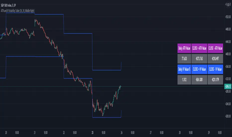
ATR and IV Volatility TableThis is a volatility tool designed to get the daily bottom and top values calculated using a daily ATR and IV values.
ATR values can be calculated directly, however for IV I recommend to take the values from external sources for the asset that you want to trade.
Regarding of the usage, I always recommend to go at the end of the previous close day of the candle(with replay function) or beginning of the daily open candle and get the expected values for movements.
For example for 26April for SPX, we have an ATR of 77 points and the close of the candle was 4296.
So based on ATR for 27 April our TOP is going to be 4296 + 77 , while our BOT is going to be 4296-77
At the same time lets assume the IV for today is going to be around 25% -> this is translated to 25 / (sqrt (252)) = 1.57 aprox
So based on IV our TOP is going to be 4296 + 4296 * 0.0157 , while our BOT is going to be 4296 - 4296 * 0.0157
I found out from my calculations that 80-85% of the times these bot and top points act as an amazing support and resistence points for day trading, so I fully recommend you to start including them into your analysis.
If you have any questions let me know !
rv_iv_vrpThis script provides realized volatility (rv), implied volatility (iv), and volatility risk premium (vrp) information for each of CBOE's volatility indices. The individual outputs are:
- Blue/red line: the realized volatility. This is an annualized, 20-period moving average estimate of realized volatility--in other words, the variability in the instrument's actual returns. The line is blue when realized volatility is below implied volatility, red otherwise.
- Fuchsia line (opaque): the median of realized volatility. The median is based on all data between the "start" and "end" dates.
- Gray line (transparent): the implied volatility (iv). According to CBOE's volatility methodology, this is similar to a weighted average of out-of-the-money ivs for options with approximately 30 calendar days to expiration. Notice that we compare rv20 to iv30 because there are about twenty trading periods in thirty calendar days.
- Fuchsia line (transparent): the median of implied volatility.
- Lightly shaded gray background: the background between "start" and "end" is shaded a very light gray.
- Table: the table shows the current, percentile, and median values for iv, rv, and vrp. Percentile means the value is greater than "N" percent of all values for that measure.
-----
Volatility risk premium (vrp) is simply the difference between implied and realized volatility. Along with implied and realized volatility, traders interpret this measure in various ways. Some prefer to be buying options when there volatility, implied or realized, reaches absolute levels, or low risk premium, whereas others have the opposite opinion. However, all volatility traders like to look at these measures in relation to their past values, which this script assists with.
By the way, this script is similar to my "vol premia," which provides the vrp data for all of these instruments on one page. However, this script loads faster and lets you see historical data. I recommend viewing the indicator and the corresponding instrument at the same time, to see how volatility reacts to changes in the underlying price.

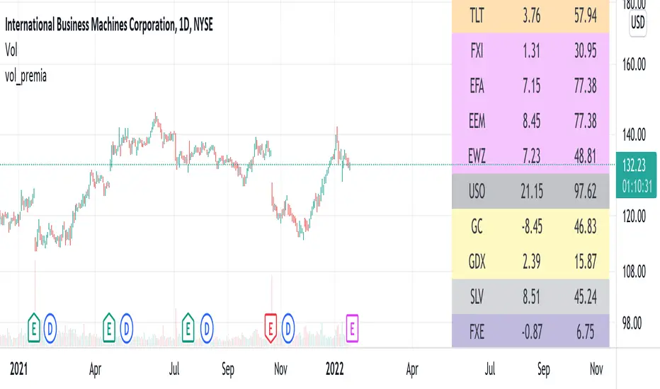
vol_premiaThis script shows the volatility risk premium for several instruments. The premium is simply "IV30 - RV20". Although Tradingview doesn't provide options prices, CBOE publishes 30-day implied volatilities for many instruments (most of which are VIX variations). CBOE calculates these in a standard way, weighting at- and out-of-the-money IVs for options that expire in 30 days, on average. For realized volatility, I used the standard deviation of log returns. Since there are twenty trading periods in 30 calendar days, IV30 can be compared to RV20. The "premium" is the difference, which reflects market participants' expectation for how much upcoming volatility will over- or under-shoot recent volatility.
The script loads pretty slow since there are lots of symbols, so feel free to delete the ones you don't care about. Hopefully the code is straightforward enough. I won't list the meaning of every symbols here, since I might change them later, but you can type them into tradingview for data, and read about their volatility index on CBOE's website. Some of the more well-known ones are:
ES: S&P futures, which I prefer to the SPX index). Its implied volatility is VIX.
USO: the oil ETF representing WTI future prices. Its IV is OVX.
GDX: the gold miner's ETF, which is usually more volatile than gold. Its IV is VXGDX.
FXI: a china ETF, whose volatility is VXFXI.
And so on. In addition to the premium, the "percentile" column shows where this premium ranks among the previous 252 trading days. 100 = the highest premium, 0 = the lowest premium.
vx_termsUSAGE
--------
This script helps train your intuition for changes in the VX term structure. I recommend using it on the VIX chart, so you can compare changes in the terms to changes in VIX. It's also nice for calendar spread traders who want to get a feel for the same changes.
1. Select a day, month, and year using the inputs
2. Observe the data table.
3. Open the input again and increment or decrement the day (and month, year as necessary).
4. Click "Ok".
5. Click to deselect the indicator, which allows the chart to load new data.
6. The data table will be reloaded with the next/previous day's data.
The data table has the following columns:
- contract: the VX contracts, in sequence. refer to the CBOE for month codes (F for January, etc.)
- close: the closing price of the contract.
- ma:mb: the spread (difference) between this row and the next row.
- ma:mb chg: the spread's change from prior close.
For example, given the following values for the first two columns:
VXQ2021, 16.5, -3.1, -0.2
VXU2021, 19.6, ..., ...
The front month (Q = august) closed at 16.5, $3.1 below the s\September contract. The negative spread enlarged by $0.20 from $2.90 on the previous trading day.
BUGS, ODDITIES, AND LIMITATIONS:
-------------------------------------------
- The first column will be greyed out after expiration day, which is the 3rd Tuesday of that month. Unfortunately, I can't load the next month's contract due to some limitations with TV.
- The active date is highlighted with a yellow background. When a non-trading date is selected, the highlight will disappear. However, the data table will sometimes fill with the nearest trading date, prematurely. No worries, just know that the data is probably for the previous Friday.
- The script is clunky and slow, but this is the best I can do with TV. Hopefully they add more continuous contracts or allow true dynamic symbol loading.
SPECIAL THANKS:
---------------------
Thanks to HeWhoMustNotBeNamed for helping me get through some messiness. Very helpful guy.
www.tradingview.com

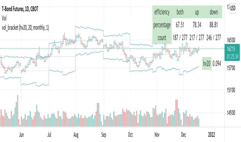
vol_bracketThis simple script shows an "N" standard deviation volatility bracket, anchored at the opening price of the current month, week, or quarter. This anchor is meant to coincide roughly with the expiration of options issued at the same interval. You can choose between a manually-entered IV or the hv30 volatility model.
Unlike my previous scripts, which all show the volatility bracket as a rolling figure, the anchor helps to visualize the volatility estimate in relation to price as it ranges over the (approximate) lifetime of a single, real contract.
VIX Implied Move Bands for ES/Emini futuresThis script uses the close of the VIX on a daily resolution to provide the 'implied move' for the E-mini SP500 futures. While it can be applied to any equity index, it's crucial to know that the VIX is calculated using SPX options, and may not reflect the implied volatility of other indices. The user can adjust the length of the moving average used to calculate the bands, the window of days used to calculate the implied move, and the multiplier that effects the width of the bands.

VIX Term StructureThis script allows users to visualize the state of the VIX Futures Term Structure. The user is able to select from five CBOE VIX Indices; VIX, VIX9D, VIX3M, VIX6M, and VIX1Y and the script will color the candles based on the price relationship between selected indices. Visit the CBOE website for more info on how the various VIX indices are calculated.

Implied Volatility PercentileThis script calculates the Implied Volatility (IV) based on the daily returns of price using a standard deviation. It then annualizes the 30 day average to create the historical Implied Volatility. This indicator is intended to measure the IV for options traders but could also provide information for equities traders to show how price is extended in the expected price range based on the historical volatility.
The IV Rank (Green line) is then calculated by looking at the high and low volatility over the number of days back specified in the input parameter, default is 252 (trading days in 1 year) and then calculating the rank of the current IV compared to the High and Low. This is not as reliable as the IV Percentile as the and extreme high or low could have a side effect on the ranking but it is included for those that want to use.
The IV Percentile is calculated by counting the number of days below the current IV, then returns this as a % of the days back in the input
You can adjust the number of days back to check the IV Rank & IV Percentile if you are not wanting to look back a whole year.
This will only work on Daily or higher timeframe charts.

IV/HV Ratio's [Nic]IV is implied volatility
HV is historic realized volatility
Seneca teaches that we often suffer more in our minds than in reality, and the same is true with the stock market. This indicator can help identify when people are over paying for implied volatility relative to real volatility . This means that short sellers are over paying for puts and can be squeezed into covering their positions, resulting in a massive rally.
The indicator can track this spread over many time frames, when the short time frame is much higher than the lower time frames, consider it a signal-of-interest.

Implied Volatility SuiteThis is an updated, more robust, and open source version of my 2 previous scripts : "Implied Volatility Rank & Model-Free IVR" and "IV Rank & IV Percentile".
This specific script provides you with 4 different types of volatility data: 1)Implied volatility, 2) Implied Volatility Rank, 3)Implied Volatility Percentile, 4)Skew Index.
1) Implied Volatility is the market's forecast of a likely movement, usually 1 standard deviation, in a securities price.
2) Implied Volatility Rank, ranks IV in relation to its high and low over a certain period of time. For example if over the past year IV had a high of 20% and a low of 10% and is currently 15%; the IV rank would be 50%, as 15 is 50% of the way between 10 & 20. IV Rank is mean reverting, meaning when IV Rank is high (green) it is assumed that future volatility will decrease; while if IV rank is low (red) it is assumed that future volatility will increase.
3) Implied Volatility Percentile ranks IV in relation to how many previous IV data points are less than the current value. For example if over the last 5 periods Implied volatility was 10%,12%,13%,14%,20%; and the current implied volatility is 15%, the IV percentile would be 80% as 4 out of the 5 previous IV values are below the current IV of 15%. IV Percentile is mean reverting, meaning when IV Percentile is high (green) it is assumed that future volatility will decrease; while if IV percentile is low (red) it is assumed that future volatility will increase. IV Percentile is more robust than IV Rank because, unlike IV Rank which only looks at the previous highs and lows, IV Percentile looks at all data points over the specified time period.
4)The skew index is an index I made that looks at volatility skew. Volatility Skew compares implied volatility of options with downside strikes versus upside strikes. If downside strikes have higher IV than upside strikes there is negative volatility skew. If upside strikes have higher IV than downside strikes then there is positive volatility skew. Typically, markets have a negative volatility skew, this has been the case since Black Monday in 1987. All negative skew means is that projected option contract prices tend to go down over time regardless of market conditions.
Additionally, this script provides two ways to calculate the 4 data types above: a)Model-Based and b)VixFix.
a) The Model-Based version calculates the four data types based on a model that projects future volatility. The reason that you would use this version is because it is what is most commonly used to calculate IV, IV Rank, IV Percentile, and Skew; and is closest to real world IV values. This version is what is referred to when people normally refer to IV. Additionally, the model version of IV, Rank, Percentile, and Skew are directionless.
b) The VixFix version calculates the four data types based on the VixFix calculation. The reason that you would use this version is because it is based on past price data as opposed to a model, and as such is more sensitive to price action. Additionally, because the VixFix is meant to replicate the VIX Index (except it can be applied to any asset) it, just like the real VIX, does have a directional element to it. Because of this, VixFix IV, Rank, and Percentile tend to increase as markets move down, and decrease as markets move up. VixFix skew, on the other hand, is directionless.
How to use this suite of tools:
1st. Pick the way you want your data calculated: either Model-Based or VixFix.
2nd. Input the various length parameters according to their labels:
If you're using the model-based version and are trading options input your time til expiry, including weekends and holidays. You can do so in terms of days, hours, and minutes. If you're using the model-based version but aren't trading options you can just use the default input of 365 days.
If you're using the VixFix version, input how many periods of data you want included in the calculation, this is labeled as "VixFix length". The default value used in this script is 252.
3rd. Finally, pick which data you want displayed from the dropdown menu: Implied Volatility, IV Rank, IV Percentile, or Volatility Skew Index.

Black-Scholes Options Pricing ModelThis is an updated version of my "Black-Scholes Model and Greeks for European Options" indicator, that i previously published. I decided to make this updated version open-source, so people can tweak and improve it.
The Black-Scholes model is a mathematical model used for pricing options. From this model you can derive the theoretical fair value of an options contract. Additionally, you can derive various risk parameters called Greeks. This indicator includes three types of data: Theoretical Option Price (blue), the Greeks (green), and implied volatility (red); their values are presented in that order.
1) Theoretical Option Price:
This first value gives only the theoretical fair value of an option with a given strike based on the Black-Scholes framework. Remember this is a model and does not reflect actual option prices, just the theoretical price based on the Black-Scholes model and its parameters and assumptions.
2)Greeks (all of the Greeks included in this indicator are listed below):
a)Delta is the rate of change of the theoretical option price with respect to the change in the underlying's price. This can also be used to approximate the probability of your option expiring in the money. For example, if you have an option with a delta of 0.62, then it has about a 62% chance of expiring in-the-money. This number runs from 0 to 1 for Calls, and 0 to -1 for Puts.
b)Gamma is the rate of change of delta with respect to the change in the underlying's price.
c)Theta, aka "time decay", is the rate of change in the theoretical option price with respect to the change in time. Theta tells you how much an option will lose its value day by day.
d) Vega is the rate of change in the theoretical option price with respect to change in implied volatility .
e)Rho is the rate of change in the theoretical option price with respect to change in the risk-free rate. Rho is rarely used because it is the parameter that options are least effected by, it is more useful for longer term options, like LEAPs.
f)Vanna is the sensitivity of delta to changes in implied volatility . Vanna is useful for checking the effectiveness of delta-hedged and vega-hedged portfolios.
g)Charm, aka "delta decay", is the instantaneous rate of change of delta over time. Charm is useful for monitoring delta-hedged positions.
h)Vomma measures the sensitivity of vega to changes in implied volatility .
i)Veta measures the rate of change in vega with respect to time.
j)Vera measures the rate of change of rho with respect to implied volatility .
k)Speed measures the rate of change in gamma with respect to changes in the underlying's price. Speed can be used when evaluating delta-hedged and gamma hedged portfolios.
l)Zomma measures the rate of change in gamma with respect to changes in implied volatility . Zomma can be used to evaluate the effectiveness of a gamma-hedged portfolio.
m)Color, aka "gamma decay", measures the rate of change of gamma over time. This can also be used to evaluate the effectiveness of a gamma-hedged portfolio.
n)Ultima measures the rate of change in vomma with respect to implied volatility .
o)Probability of Touch, is not a Greek, but a metric that I included, which tells you the probability of price touching your strike price before expiry.
3) Implied Volatility:
This is the market's forecast of future volatility . Implied volatility is directionless, it cannot be used to forecast future direction. All it tells you is the forecast for future volatility.
How to use this indicator:
1st. Input the strike price of your option. If you input a strike that is more than 3 standard deviations away from the current price, the model will return a value of n/a.
2nd. Input the current risk-free rate.(Including this is optional, because the risk-free rate is so small, you can just leave this number at zero.)
3rd. Input the time until expiry. You can enter this in terms of days, hours, and minutes.
4th.Input the chart time frame you are using in terms of minutes. For example if you're using the 1min time frame input 1, 4 hr time frame input 480, daily time frame input 1440, etc.
5th. Pick what style of option you want data for, European Vanilla or Binary.
6th. Pick what type of option you want data for, Long Call or Long Put.
7th . Finally, pick which Greek you want displayed from the drop-down list.
*Remember the Option price presented, and the Greeks presented, are theoretical in nature, and not based upon actual option prices. Also, remember the Black-Scholes model is just a model based upon various parameters, it is not an actual representation of reality, only a theoretical one.
*Note 1. If you choose binary, only data for Long Binary Calls will be presented. All of the Greeks for Long Binary Calls are available, except for rho and vera because they are negligible.
*Note 2. Unlike vanilla european options, the delta of a binary option cannot be used to approximate the probability of the option expiring in-the-money. For binary options, if you want to approximate the probability of the binary option expiring in-the-money, use the price. The price of a binary option can be used to approximate its probability of expiring in-the-money. So if a binary option has a price of $40, then it has approximately a 40% chance of expiring in-the-money.
*Note 3. As time goes on you will have to update the expiry, this model does not do that automatically. So for example, if you originally have an option with 30 days to expiry, tomorrow you would have to manually update that to 29 days, then the next day manually update the expiry to 28, and so on and so forth.
There are various formulas that you can use to calculate the Greeks. I specifically chose the formulations included in this indicator because the Greeks that it presents are the closest to actual options data. I compared the Greeks given by this indicator to brokerage option data on a variety of asset classes from equity index future options to FX options and more. Because the indicator does not use actual option prices, its Greeks do not match the brokerage data exactly, but are close enough.
I may try to make future updates that include data for Long Binary Puts, American Options, Asian Options, etc.


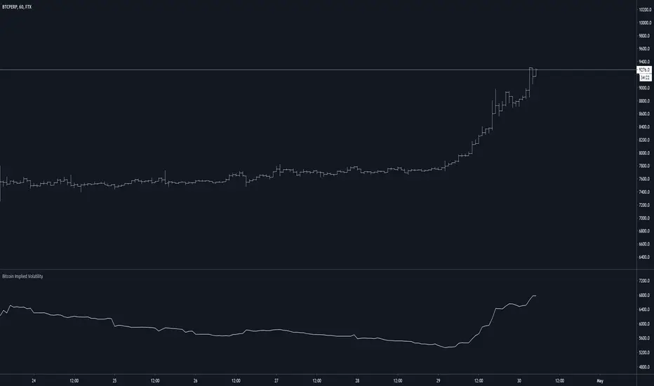
Bitcoin Implied VolatilityThis simple script collects data from FTX:BVOLUSD to plot BTC’s implied volatility as a standalone indicator instead of a chart.
Implied volatility is used to gauge future volatility and often used in options trading.
SPY Expected Move by VIXThis indicator shows 1 and 2 standard deviation price move from the VWAP based on VIX. Implied Volatility (IV) is being used extensively in the Option world to project the Expected Move for the underlying instrument. VIX is used as a proxy for SPY's IV for 30 days.
This indicator is meaningful only for SPY but can be used in any other instrument which has a strong correlation to SPY.

IV/HV ratio 1.0 [dime]This script compares the implied volatility to the historic volatility as a ratio.
The plot indicates how high the current implied volatility for the next 30 days is relative to the actual volatility realized over the set period. This is most useful for options traders as it may show when the premiums paid on options are over valued relative to the historic risk.
The default is set to one year (252 bars) however any number of bars can be set for the lookback period for HV.
The default is set to VIX for the IV on SPX or SPY but other CBOE implied volatility indexes may be used. For /CL you have OVX/HV and for /GC you have GVX/HV.
Note that the CBOE data for these indexes may be delayed and updated EOD
and may not be suitable for intraday information. (Future versions of this script may be developed to provide a realtime intraday study. )
There is a list of many volatility indexes from CBOE listed at:
www.cboe.com
(Some may not yet be available on Tradingview)
RVX Russell 2000
VXN NASDAQ
VXO S&P 100
VXD DJIA
GVX Gold
OVX OIL
VIX3M 3-Month
VIX6M S&P 500 6-Month
VIX1Y 1-Year
VXEFA Cboe EFA ETF
VXEEM Cboe Emerging Markets ETF
VXFXI Cboe China ETF
VXEWZ Cboe Brazil ETF
VXSLV Cboe Silver ETF
VXGDX Cboe Gold Miners ETF
VXXLE Cboe Energy Sector ETF
EUVIX FX Euro
JYVIX FX Yen
BPVIX FX British Pound
EVZ Cboe EuroCurrency ETF Volatility Index
Amazon VXAZN
Apple VXAPL
Goldman Sachs VXGS
Google VXGOG
IBM VXIBM
