S&P500 Can the 1D MA50 save the day?The S&P500 index (SPX) has been trading within a 5-month Channel Up and last Friday's flash crash touched its bottom making a new Higher Low. At the same time, it hit its 1D MA50 (blue trend-line) for the first time May 01 2025.
As long as the market keeps closing the daily candles inside the Channel Up, we expect the new Bullish Leg to start and as the shortest ones did within the pattern, target at least the 1.382 Fibonacci extension level at 6850.
If a 1D candle closes below the Channel Up though, there are higher probabilities to see a stronger dip to the 1D MA100 (green trend-line) a 6400.
On a sidenote, the 1D RSI hit and rebounded on Friday on its Lower Lows trend-line, favoring at the moment a bullish continuation.
-------------------------------------------------------------------------------
** Please LIKE 👍, FOLLOW ✅, SHARE 🙌 and COMMENT ✍ if you enjoy this idea! Also share your ideas and charts in the comments section below! This is best way to keep it relevant, support us, keep the content here free and allow the idea to reach as many people as possible. **
-------------------------------------------------------------------------------
💸💸💸💸💸💸
👇 👇 👇 👇 👇 👇
Trade ideas

SPX500 Slips Below Pivot as Sellers Regain ControlSPX500 – Overview | Bearish Bias Below 6,609
The index reversed lower from resistance around 6,672 and has now stabilized below the pivot line at 6,609, signaling a continuation of bearish momentum.
As long as price trades below 6,609, the trend remains bearish, targeting 6,577 → 6,550, with further downside potential toward 6,507.
A 1H close above 6,609 would negate the bearish setup and shift momentum bullish toward 6,635 → 6,672 → 6,700.
Pivot: 6,609
Support: 6,577 – 6,550 – 6,507
Resistance: 6,635 – 6,672 – 6,700

S&P500 Volatility remains elevated, ahead of earnings resultsMonday’s Rally Recap:
The S&P 500 rebounded strongly, recovering over half of Friday’s losses. The main driver was more positive trade rhetoric, with signs the US is open to compromise—softening the tone from Friday’s comments.
A secondary boost came from AI optimism, as OpenAI signed a major chip deal with Broadcom (+9.88%), lifting tech sentiment.
Current Market Setup:
Despite Monday’s gains, S&P 500 futures are down -0.38% this morning, as:
US-China tensions escalated again—China sanctioned US units of a Korean shipping giant, a counter to US trade pressure.
Market volatility persists, with the dollar and Treasuries rising, and oil pulling back.
Government shutdown enters Day 14, disrupting IPO timelines and withholding macroeconomic data, adding uncertainty.
Focus Ahead:
The start of US earnings season today is crucial: JPMorgan, Goldman Sachs, Wells Fargo, BlackRock, Citigroup, and Johnson & Johnson all report. Their results will likely set the tone for Q4 expectations and influence near-term direction.
Underneath market movements, there's a sense of longer-term repricing as investors hedge against policy uncertainty and inflation ("debasement trade").
Bottom Line for S&P 500:
Volatility remains elevated. Monday’s rebound was fueled by sentiment, but renewed geopolitical risk, lack of macro data, and earnings uncertainty are keeping futures under pressure today. Market likely to trade cautiously until earnings results provide clearer direction.
Key Support and Resistance Levels
Resistance Level 1: 6680
Resistance Level 2: 6703
Resistance Level 3: 6728
Support Level 1: 6547
Support Level 2: 6522
Support Level 3: 6487
This communication is for informational purposes only and should not be viewed as any form of recommendation as to a particular course of action or as investment advice. It is not intended as an offer or solicitation for the purchase or sale of any financial instrument or as an official confirmation of any transaction. Opinions, estimates and assumptions expressed herein are made as of the date of this communication and are subject to change without notice. This communication has been prepared based upon information, including market prices, data and other information, believed to be reliable; however, Trade Nation does not warrant its completeness or accuracy. All market prices and market data contained in or attached to this communication are indicative and subject to change without notice.

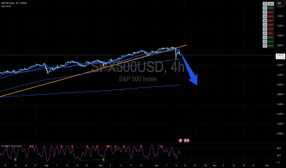
$SPX Sell is not over yetHuge down move on Friday on Trump's tweet. And a gap up yesterday and market was sideways. So we are going up from here? It was a super bearish candle on Friday and technical points to further downside.
Indeed, my call at 840pm EST timestamped was followed by a 80 pts sell down. I could be wrong but I see 6000 or so; confluence of support, and even down to 5800 (50 Fib) before a huge rally towards end of year.
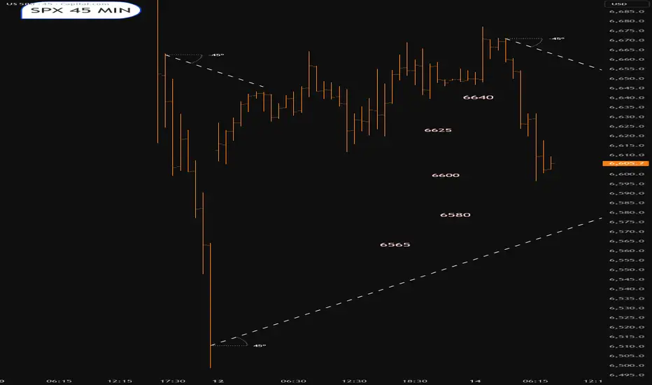
SPX into the Euro open.Tuesday 14th OctoberPoss supp area 6565-6600 looming
66400 seems to be some swearing and fighting
From 'pullbacks' to a 'correction' (S&P 500)Setup
Still Bullish. Be patient for entry near end of the corrective move lower
Evidence..
-Trend is up, no top pattern
-No longer 'dips' to 50 DMA, now into a 'correction' with possible move towards 100 DMA
-Large bearish engulfing weekly candle
-The 4 month old trendline has broken.
-RSI has dropped under support - but not yet characteristic of bearish trend by going oversold
-Price has landed at a demand zone under 6500 (could rebound from here)
Signal
Looking to go long on another test of the demand zone OR
at next supports found at matching lows of 6350 then 6200

SPX | Daily Analysis #2Hello and welcome back to DP,
**Review and News**
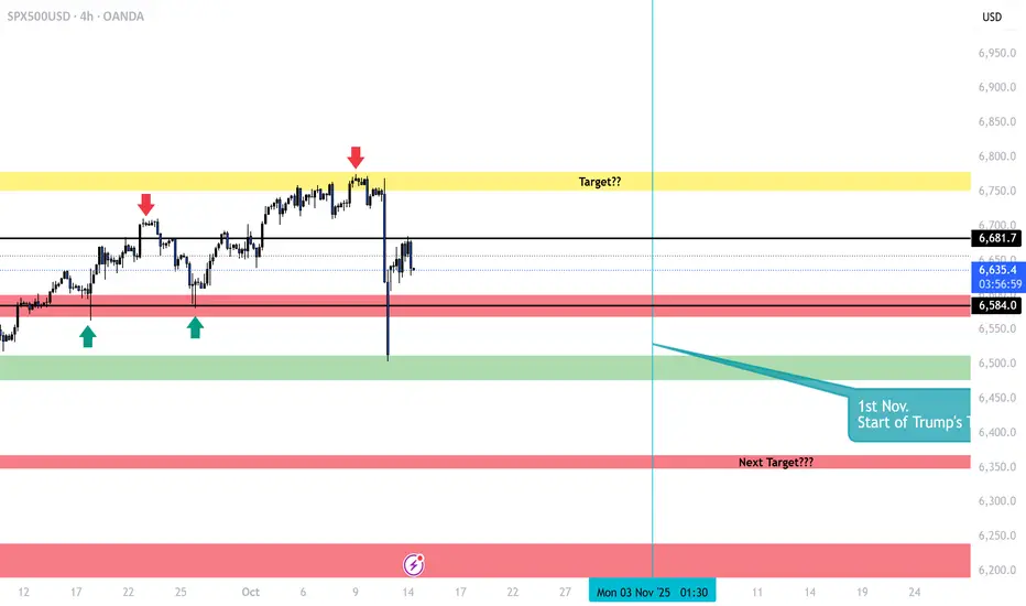
Yesterday, at the start of the week, the SPX opened with a significant upside gap, largely driven by a tweet from former President Trump on Friday. His statement—"Don’t worry about China and Xi, they don’t want a recession for their economy, and neither do we"—helped restore investor confidence, pushing them back into the market, particularly into this index. However, shortly after, Trump reiterated that tariffs would still be implemented on November 1st, which is expected to have a considerable impact.
This morning, President Xi reaffirmed his stance, saying, "China will fight to the end, but the doors for negotiation are always open." As seen on the chart, the price has moved within a range between $6,681 and $6,584.
**4-Hour Price Action**
As indicated by the chart, the price range between $6,681 and $6,584 seems to be holding steady for now. One scenario suggests the market is in a consolidation phase. The shape of this consolidation will depend on the future performance of the market. It could either form a diagonal pattern or remain within a box range, as investors battle against short-sellers.
Using Fibonacci retracement, it appears the price may extend to the 0.236 line at $6,706. If this Fibonacci level holds, the market could face a downturn, potentially targeting the next support level indicated by the red box below the chart.
**Trend Analysis**
As shown, the trend illustrates a clear relationship with price movement. The price opened above the trend line, then expanded below the next trend level, showing respect for it. This movement suggests that downward pressure remains, with the market's direction depending on the break of the current trend line.
Personally , I believe the market may head south, but it won’t be a straightforward move. The decline could be unpredictable and happen quickly, or it may unfold in more gradual, choppy moves. One thing to be certain of is that retail traders are betting against the market, mainly due to the gap being filled. However, caution is advised when trading this index. It’s important to wait for confirmation before making any decisions.
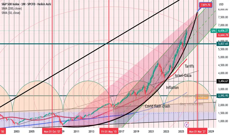
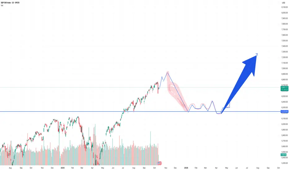
15% uptrend until March 2027Just have a look.
The market is in an incredible bull run since 2009. Its move is parabolic and it will probably end around 8000 pips in March 2027.
My theory is based in the bottoms of this cycles:
2008-2015-2020-2023-2025 or in other words:
Finantial crisis.
Covid
Israel Conflict
Trump´s Tariffs.
Other indicators are Gann cycles which collide in the exact points.
Therefore, my idea is to see Sp500 at 7800 points in March 2027 before seeing the huge crash that it must be needed to cool off after almost 20 years of bull run.
SNP500 short uptick and quick downfallZeusExodus
As the marked upticks close to 7k levels it will drop about 10% that will mark the lowest point on July 11th.
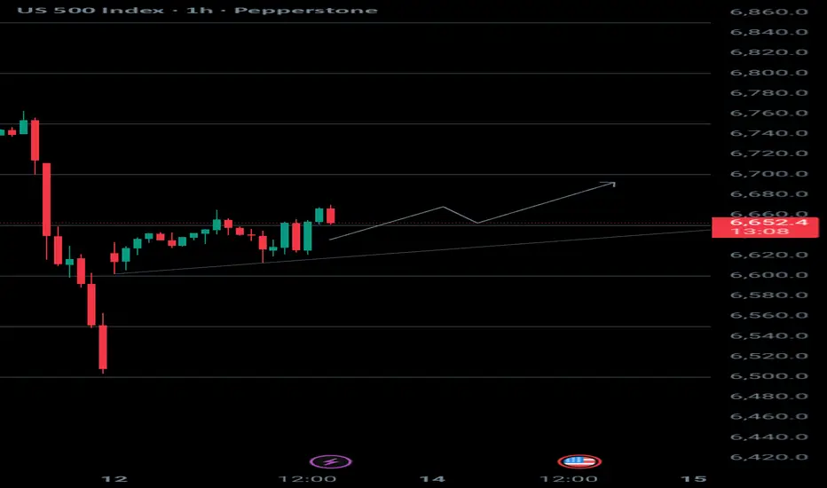
US 500The US 500 has just broken through the 6650 level again. After testing support and closing above it, the trend is to target the next level, 6700.
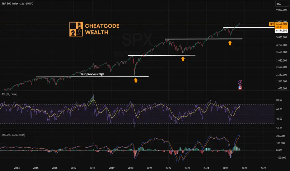
SP500 path forward: volatility and retest of previous highsAssuming that previous patterns continue, and they may not, the SP500 will eventually retest its previous new highs, but likely not in the near future, short of a volatility event.
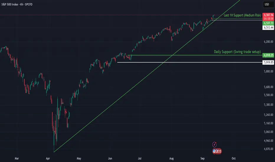
SPX Supported by Trendline and Rate Cut ExpectationsThe S&P 500 has been climbing steadily, with the ascending trendline from April acting as a reliable backbone for the move. Despite short-term volatility, buyers continue to defend higher lows. Coupled with expectations of interest rate cuts, the trend structure remains intact unless key supports give way.
🔍 Technical Analysis
Current price: 6,584
The green trendline (since April) is guiding the advance.
Price is consolidating near highs, supported by demand zones underneath.
🛡️ Support Zones & Stop-Loss (White Lines):
🟢 6,537 – 1H Support (Medium Risk)
First line of defense for short-term traders.
Stop-loss: Below 6,513
🟡 6,018 – Daily Support (Swing Trade Setup)
Stronger base for medium-term positioning.
Stop-loss: Below 5,919
🧭 Outlook
Bullish Case: Hold above 6,537 + April trendline intact → continuation toward new highs above 6,600–6,700.
Bearish Case: Break below 6,537 could trigger a correction into 6,018. Losing that zone would weaken the April trendline structure.
Bias: Bullish while April trendline holds.
🌍 Fundamental Insight
Rate cut expectations continue to provide a macro tailwind for equities. With inflation moderating and yields easing, investors remain willing to support risk assets. A sudden shift in data or Fed tone, however, could test the resilience of the April trendline.
✅ Conclusion
The S&P 500 remains in a strong bullish structure, anchored by the April trendline. Unless supports at 6,537 or 6,018 are lost, the path of least resistance remains higher.
If you found this useful, please don’t forget to like and follow for more structure-based insights.
⚠️ Disclaimer
This analysis is for educational purposes only and does not constitute financial, investment, or trading advice.
S&P 500 (SPX) Simple Break Down The S&P (SPX) is sitting at a key turning point. Here’s what to watch for next:
If price drops below 6553, we could see it keep falling toward 6469 and if that breaks, then possibly down to around 6398.
But if price pushes above 6763, the next big target area could be 7237–7274.
So basically:
👉 Below 6553 = likely drop
👉 Above 6763 = likely climb
Right now, we’re in a tight spot where either direction could open up a strong move.
If you’re unsure how to trade around these levels or what kind of pullback makes sense, shoot me a quick DM
I can walk you through how I’m looking at setups and risk zones in plain English.
Mindbloome Exchange

S&P 500: TACO Trump or Something More Serious?After a summer of plain sailing for the S&P 500, Friday’s sell-off was the first market wobble we’ve witnessed in some time. Let’s take a look at what this means moving forward…
Tariff Turbulence Returns
Donald Trump’s latest tariff threats against China sent shockwaves through markets on Friday, triggering the S&P 500’s biggest one-day drop since April. His comments, accusing Beijing of becoming “very hostile” and vowing “massive” tariffs, reignited fears of a full-blown trade war. Investors rushed into safe havens, pushing Treasury yields lower and sending gold back toward record highs. The sell-off saw more than four in five stocks in the index finish in the red, bringing an abrupt pause to the market’s recent record-breaking run.
But as Wall Street traders know, Trump’s tariff threats don’t always end the way they start. The “Trump Always Chickens Out” or TACO trade has become a familiar playbook for traders who buy the dip after a tariff announcement, then sell the rebound when the president softens his tone. Sure enough, over the weekend Trump hinted at reconciliation, praising President Xi and calling for cooperation. That shift helped US futures rebound early Monday, as investors once again bet that the sell-off might be more bark than bite. The question now is whether this episode follows the usual TACO script or signals something deeper brewing beneath the surface.
Bearish Engulfing Shock Sets the Parameters
Friday’s daily candle tells the story best. The huge bearish engulfing candle didn’t just erase the prior week’s gains, it wrapped around several days of price action and signalled a sharp shift in sentiment. Its sheer size is significant because range expansion after a calm period often marks a turning point in market psychology. The candle’s lower wick, finding support near the 50-day moving average, shows that buyers did emerge at key trend support, but how price behaves within this range will now define the path forward.
US500 Daily Candle Chart
Past performance is not a reliable indicator of future results
The hourly chart shows how that panic played out and how quickly traders have tried to repair the damage. The market found support before gapping higher at Monday’s open, showing a tentative attempt to stabilise. This kind of response often reveals whether a sell-off was a genuine trend reversal or a momentary flush of emotion. If price can keep grinding higher from here and close back above the midpoint of Friday’s engulfing candle, it would confirm that the uptrend remains intact and that buyers still have control.
However, if the S&P 500 stalls or consolidates in the lower half of that candle’s range, it would be a clear warning that the market’s tone has changed. Sideways price action here would imply that traders are waiting for confirmation rather than chasing rebounds, and that shift in behaviour can often lead to a second leg lower. The size of Friday’s engulfing candle now marks a battleground between short-term buyers and cautious longer-term investors. Whether we see a swift recovery or a slow grind will reveal if this was just another TACO moment or the start of something more meaningful.
US500 Hourly Candle Chart
Past performance is not a reliable indicator of future results
Disclaimer: This is for information and learning purposes only. The information provided does not constitute investment advice nor take into account the individual financial circumstances or objectives of any investor. Any information that may be provided relating to past performance is not a reliable indicator of future results or performance. Social media channels are not relevant for UK residents.
Spread bets and CFDs are complex instruments and come with a high risk of losing money rapidly due to leverage. 85.24% of retail investor accounts lose money when trading spread bets and CFDs with this provider. You should consider whether you understand how spread bets and CFDs work and whether you can afford to take the high risk of losing your money.

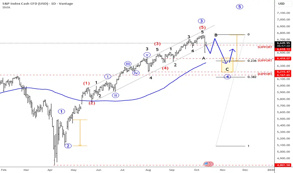
SP500: Breaks Out Of Channel, Steps Into Wave Four I hope you had a nice weekend despite that nasty turn lower on stocks we saw on Friday. As you know, the move came after Trump threatened to impose new tariffs on China, following China’s own restrictions and tighter export controls on rare earth metals, which are crucial for the tech sector. We’ve seen this story before back in April, and if tariffs come back into focus again, traders will likely react with fear — so it’s not a surprise we saw such a strong drop in stocks on Friday.
Normally, markets are most sensitive when this kind of news first hits, and then they tend to stabilize afterward. What’s interesting, though, is that despite the strong sell-off in stocks, the dollar index didn’t show the kind of sharp upside reaction you’d usually expect. So I’m wondering if stocks can find some support, but seems like this can be only wave B rally, since we are in the middle of wave four retracement. Keep in mind there is an open gap lower on futures.
Big supports is at 6400 and 6200.
Grega
I can't believe nowbody saw this coming for crypto. S&P 500 Technical Analysis: Long-Term Channel Pattern
The S&P 500 has been trading within a well-defined ascending parallel channel for over 5 years. As shown in the chart, the index has consistently respected both the upper resistance and lower support trendlines of this channel throughout this period.
Current Market Position:
The index recently reached the upper boundary of this parallel channel around the 6,700-6,800 level and has begun to pull back. Historically, when the S&P 500 has tested this upper resistance line, it has typically reversed and moved toward the lower support trendline.
Key Observations:
Channel Behavior: The price action shows a clear pattern of rejection at the upper channel resistance, followed by moves back toward the middle or lower boundary of the channel.
Correlation with Crypto: When the S&P 500 experiences significant downward moves, risk assets like cryptocurrencies tend to follow suit, often with amplified volatility.
Potential Scenarios: While a retest of the upper resistance is possible, the more probable scenario based on historical channel behavior is a move toward the lower support line, which currently sits around the 5,200-5,400 range.
Risk Factors:
The current market environment faces additional headwinds, particularly concerns about an AI bubble. If sentiment shifts regarding AI valuations, this could accelerate the move toward channel support, as AI-related stocks have been significant drivers of the index's recent performance.
Conclusion:
Technical analysis suggests caution at current levels, with the channel's upper boundary acting as a natural resistance zone. Risk management and monitoring of support levels will be crucial in the coming weeks.

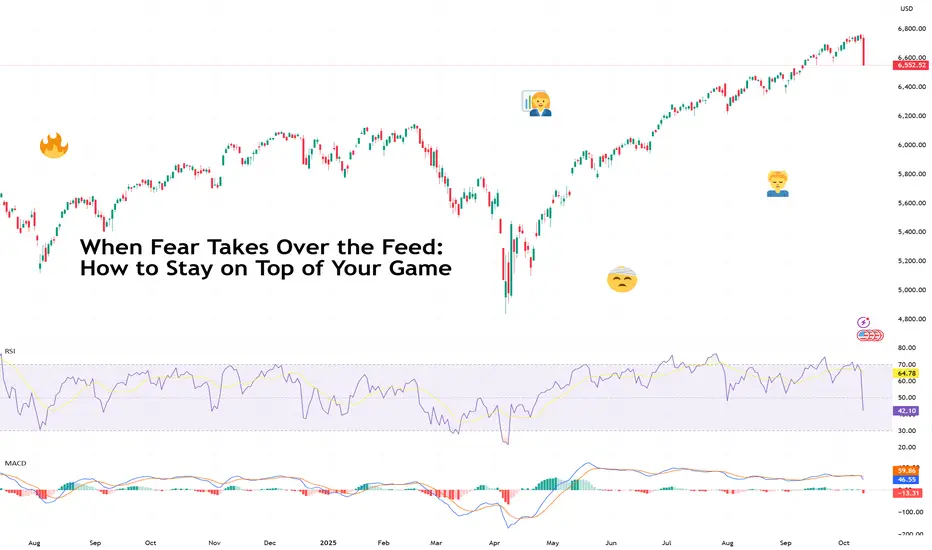
When Fear Takes Over the Feed: How to Stay on Top of Your GameFriday wasn’t just a red day — it was the kind of red that makes traders question their life choices.
The Nasdaq Composite NASDAQ:IXIC plunged 3.6% , its worst day since the April tariff-fueled meltdown.
The S&P 500 SP:SPX dropped 2.7%, the Dow Jones TVC:DJI tumbled nearly 900 points, and $1.6 trillion in market value simply evaporated.
Hello tariffs, my old friend.
President Trump announced he’s canceling a planned meeting with China’s Xi Jinping and slapping 100% tariffs on Chinese goods. Just when investors thought the trade wars were over.
It was China this time that triggered the mayhem. President Xi unveiled plans to tighten controls on rare-earth exports, materials critical for EVs and high-tech hardware.
The widespread selling was especially brutal over at the crypto corner with a record $19 billion in liquidations. Bitcoin BITSTAMP:BTCUSD face-planted 7.2% for the day, sliding below $111,000.
So, what’s a trader supposed to do when markets melt faster than your enthusiasm to study the Elliott wave?
Here’s a step-by-step guide that breaks down the psychology of panic and how smart traders stay cool when the feed turns into a fear factory.
🧠 Step One: Understand the “Fear Reflex”
When bad news breaks, the first instinct for most traders is to actually do something. Anything. Sell, short, hedge, pray — anything to make the pain stop. That’s your amygdala (the brain’s alarm system) talking.
When headlines hit, ask yourself:
• Is this new information, a re-spin of old fears, or a projection?
• Does it change the fundamentals of my positions?
• What’s the time frame of this impact — minutes, months, or meme-cycle?
If you can’t answer those calmly, and instead rush to offload your positions, you’re in panic mode and you risk making impulse decisions.
📊 Step Two: Zoom Out (Literally and Mentally)
When fear takes over the feed, the chart shrinks. Traders start staring at 1-minute candles and wonder if they should dump their stocks right now .
That’s the moment to zoom out. Pull up the 4-hour, daily, or weekly chart. You’ll likely notice that Friday’s epic collapse looks less like the apocalypse and more like a blip in an ongoing uptrend.
Case in point: The Nasdaq may have tanked 3.6%, but it’s still sitting near record territory after months of AI-fueled gains. The broader trend — higher highs, higher lows — is intact.
Volatility doesn’t mean reversal. It means emotion acting out. And markets love testing conviction.
💬 Step Three: Tune Out the Noise
When every post in your feed screams “MARKET MELTDOWN!” it’s tempting to join the panic chorus. But that doesn’t mean it’s going to be like that tomorrow.
Take for example the April crash. Stocks were rising and rising , and not too long after, they started hitting record after record .
You don’t need to read 20 opinions — you need one solid plan (and, of course, to be a daily reader of our Top Stories ).
A simple checklist helps:
• Position size: Are you overexposed?
• Stop-loss: Is it placed logically, not emotionally?
• Cash buffer: Do you have dry powder for the dip?
Don’t scramble mid-freefall. Prepare for volatility before it happens.
🧩 Step Four: Identify the Difference Between Noise and Narrative
Every market drop has two layers — the market-shaking news story and how investors perceive it.
• The headline on Friday: “Trump reignites trade war with China.”
• The perception: Markets pricing growth halt, rake hikes, gloom and doom, and apocalypse.
In the short term, that’s fear-inducing. In the medium term? It could actually mean looser monetary policy — which is generally bullish for risk assets like stocks, gold, and even crypto.
In other words, what feels like the end of the world on Friday might look like a buying opportunity by Tuesday.
🧭 Step Five: Play Offense When Others Play Defense
There’s a reason Buffett’s “be fearful when others are greedy” quote is overused — because it’s true.
When the market wipes out $1.6 trillion in a day, it’s a reminder that liquidity and emotion drive short-term moves. If your thesis is intact and you’re not that up high on leverage, you may consider this drop as a time to look for opportunities.
Instead of selling in fear, study which sectors overreacted.
• Tech led the plunge — but if (or when) there’s a rebound, these stocks will most likely be the leaders. Especially now when the third-quarter earnings season is here (check when it’s big tech’s turn to report by browsing the Earnings calendar ).
• Gold and bonds saw inflows — typical defensive plays.
• Energy and industrials may catch bids if tariffs stick.
🪙 A Note to Crypto Bros
Bitcoin’s 7% slide shows that once-independent assets have spent too much time with traditional risk assets.
And now they’re almost impossible to tell apart. As institutional capital grows in crypto, it behaves more like a growth play where risk is embraced during good times, but dumped during bad.
The lesson? Don’t buy the “decoupling” narrative so easily. Bitcoin may hedge against long-term fiat decay, but in a short-term panic, it’s still part of the same risk ecosystem. The smart move is to trade correlations , not beliefs.
If Bitcoin drops with stocks during a tariff tantrum, that’s confirmation that institutional traders are playing both arenas.
🧡 Final Takeaway
Let’s acknowledge that Friday’s bloodbath was catastrophic to many . It wiped out traders that were holding both stocks and crypto. If that happened to you, as painful as it is, keep your head up, take a breath (or a break), and come back another day.
And when you do, widen your chart, trim that leverage and keep your bets nimble so you’d survive the next inevitable meltdown.
Finally, we can't not address the elephant in the room. It was likely another Trump-led market rinse-and-repeat cycle: tweet, panic, rebound. Futures are recovering after Trump waved away tariff fears , saying “Don’t worry about China, it will all be fine!”
Off to you : How did you fare Friday? And what's your way of weathering the market storms? Share your experience in the comments!
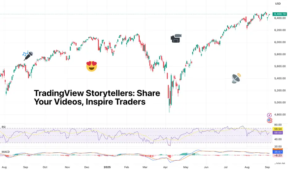
TradingView Storytellers: Share Your Videos, Inspire TradersCalling all creators, chart wizards, and video storytellers.
👋 Hey traders !
We know many of you aren’t just analyzing the markets and trading — you’re teaching, creating, and inspiring others. We see you!
And now's your chance to get your content in the spotlight — share your best work with us. Top submissions will get featured front and center for the TradingView community.
👉 How to take part:
1️⃣ Share a short video (new or one you already have) that shows how you’re using your favorite TradingView features.
2️⃣ Submit it by filling out our quick questionnaire.
That’s it! Your work could be shared with thousands of traders around the world, inspiring others and helping grow our community of creators.
🎁 As a little thank you, we’ll be gifting three free Premium annual plans to standout submissions. And who knows — you might even end up collaborating with us in the future.
👉 Fill out the questionnaire
US 500 Index – Limited Correction Or Sentiment Reversal?With all the talk in the financial press last week of a potential AI bubble, soaring volatility in the precious metals market, and an on-going US government shutdown, perhaps it was understandable that traders were a little on edge going into Friday. So, when President Trump’s new threats of 100% tariffs on China were posted on social media late in the afternoon the reaction was a big downside correction, which saw the US 500 drop around 3.6% from its all-time highs of 6769 seen just a day earlier to a low of 6508.
Since then, comments from President Trump and Vice President Vance over the weekend regarding China have seemed to be more conciliatory in tone, signalling an openness to get back to the negotiating table and hammer out a deal in some form. This has seen all markets breath a small sigh of relief and led the US 500 to open higher, currently trading up 2.2% around 6650 (0800 BST). However, whether this positivity continues may depend on multiple factors, including the technical outlook (more on this below).
While trader sensitivity to the next round of comments from the US and Chinese administrations regarding the on-going trade tensions could remain high, they may also be keen to receive the latest Q3 earnings from the major US banks, with JP Morgan, Goldman Sachs and Citigroup reporting on Tuesday (before the open), then Bank of America and Morgan Stanley reporting on Wednesday (before the open). While the focus may be on assessing actual performance against expectations, it could also be important to hear the outlook for future revenue, the direction of US economic growth and the size of bad debt provisions.
Federal Reserve Chairman Jerome Powell also speaks on Tuesday at 1720 BST and with the US government shutdown delaying the release of the most recent inflation updates (CPI/PPI) which were due this week until later in October, any comments he makes regarding the inflation outlook or the potential for an October Fed rate cut could take on extra significance.
Technical Update: Limited Correction or Sentiment Reversal?
Headline-driven price sell-offs like the one experienced on Friday (Oct 10th) are unpredictable, underscoring the importance of disciplined risk management. If you're long of an asset during such volatility, having well-placed stop-losses is crucial to limit downside exposure, especially when liquidity starts to reduce, as it likely did ahead of today’s US holiday. These events serve as a reminder that protecting your trading capital is just as important as delivering profitable outcomes.
After such a sharp sell-off, the question is whether it marks a brief, exaggerated correction within a broader uptrend or signals a deeper negative sentiment shift that could lead to further price weakness.
The answer may well depend on how the price of the US 500 reacts in the upcoming sessions. Whether support levels hold, momentum stabilises, and buyers return or whether the price decline deepens and the next support levels give way.
The jury may still be out on this, but as the chart above shows, judging the potential key support and resistance levels could help gauge the next directional risks. A closing break of either side may offer signals to the next phase of price activity.
If the Sell-Off Reflects a Negative Sentiment Shift:
Friday’s sharp decline may have already breached some initial support levels, raising the risk of a more extended phase of price weakness.
The daily Bollinger mid-average (currently 6668) is typically viewed by traders as a support level in an uptrend and this level was broken on a closing basis within Friday’s decline. Despite this morning’s rally, 6668 could now act as a resistance, and if it remains intact, could keep upside activity in check for now.
While 6668 resistance holds on a closing basis, this morning’s recovery may be viewed by some as a reactionary bounce following Friday’s sharp decline, leaving possibilities of renewed selling pressure later in the week.
If this proves to be the case, closing breaks below potential support at 6550, a level which is equal to half the rebound from Friday’s low, might lead to renewed downside pressure. This may open tests of 6490, the 50% retracement of the August 1st to October 9th rally, with a closing break below this level, suggesting scope for moves toward 6224 which is the 61.8% retracement.
If the Sell-Off Proves to be a Limited Correction:
While Friday’s decline was sharper and larger than any since the June 2025 lows, traders may now be watching whether current price strength can close back above the 6668 Bollinger mid-average.
While not a guarantee of renewed price strength, past declines since June 23rd 2025, have seen US 500 prices recover to close back above this line, leading to resumed attempts at upside strength. A closing break back above 6668 may once again open attempts to push to higher levels.
If confirmed, a break above resistance at 6668 may lead to further upside back toward 6769, which is the October 9th all-time high. Should this level give way, further strength may extend toward 6866, which is the 38.2% Fibonacci extension of last week’s sharp decline.
The material provided here has not been prepared accordance with legal requirements designed to promote the independence of investment research and as such is considered to be a marketing communication. Whilst it is not subject to any prohibition on dealing ahead of the dissemination of investment research, we will not seek to take any advantage before providing it to our clients.
Pepperstone doesn’t represent that the material provided here is accurate, current or complete, and therefore shouldn’t be relied upon as such. The information, whether from a third party or not, isn’t to be considered as a recommendation; or an offer to buy or sell; or the solicitation of an offer to buy or sell any security, financial product or instrument; or to participate in any particular trading strategy. It does not take into account readers’ financial situation or investment objectives. We advise any readers of this content to seek their own advice. Without the approval of Pepperstone, reproduction or redistribution of this information isn’t permitted.

Trump’s Decision Shakes Global Financial MarketsTrump’s Decision Shakes Global Financial Markets
On Friday, 10 October, President Trump made an unexpected statement about the possible introduction of 100% tariffs on Chinese goods, triggering sharp price swings across global markets:
→ Stock markets: The S&P 500 index tumbled by more than 3%, hitting its lowest level in over a month.
→ Currency markets: The US dollar slumped sharply against other major currencies.
However, on Sunday, Donald Trump softened his tone on Truth Social, suggesting that trade relations with Beijing “will be absolutely fine”. Vice President JD Vance echoed this sentiment, adding that the United States is ready for talks if China is “prepared to act reasonably”.
This shift in rhetoric from US officials helped markets recover, with the S&P 500 index rebounding sharply at Monday’s open, reclaiming much of Friday’s losses.
Technical Analysis of the S&P 500 Chart
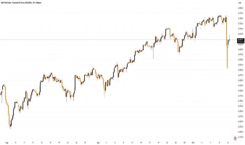
In our previous analysis of the 4-hour S&P 500 chart (US SPX 500 mini on FXOpen) on 4 October, we identified an upward channel (shown in blue) and expressed several concerns:
→ The price was approaching the upper boundary of the channel, where long positions are often closed for profit.
→ The latest peak slightly exceeded the October high (A), suggesting a potential bearish divergence.
→ The news blackout caused by the government shutdown created an “information vacuum”, which could quickly turn sentiment negative if filled with adverse developments.
The lower boundary of the blue channel offered only temporary support near 6,644 points on Friday before the price broke downwards. Doubling the channel width provides a projected target near 6,500, which coincides with Friday’s low.
Given these factors, it can be assumed that the lower line of the blue channel now acts as the median of a broader range following Friday’s sell-off. This suggests that in the coming days, the S&P 500 index may stabilise as demand and supply find temporary balance along this line.
Looking further ahead, the situation may resemble that of early April, when after a panic-driven market drop (also triggered by Trump’s tariff comments), the S&P 500 not only fully recovered but went on to reach new highs.
Key Levels:
→ 6,705 – a level that has acted as both support and resistance this autumn;
→ 6,606 – the boundary of the bullish gap.
This article represents the opinion of the Companies operating under the FXOpen brand only. It is not to be construed as an offer, solicitation, or recommendation with respect to products and services provided by the Companies operating under the FXOpen brand, nor is it to be considered financial advice.

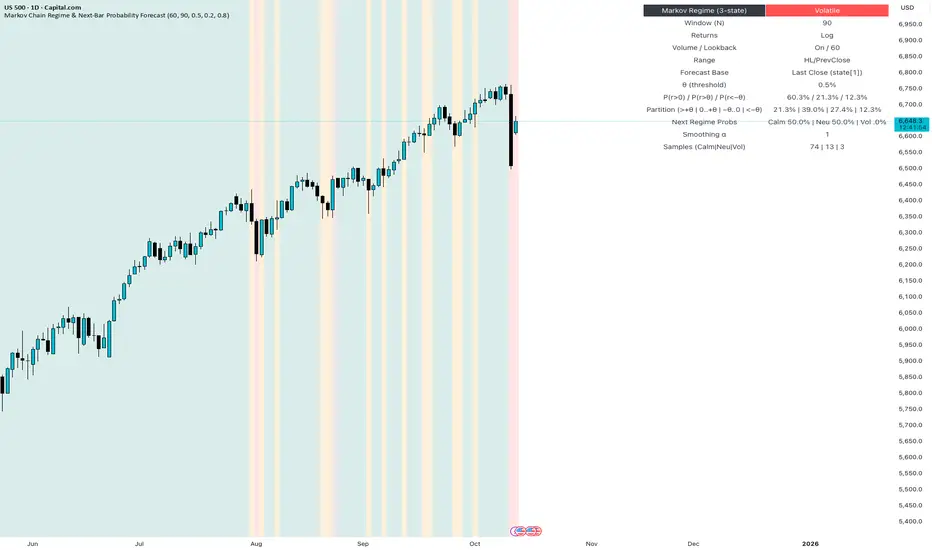
HOW-TO: Forecast Next-Bar Odds with Markov ProbCast🎯 Goal
In 5 minutes, you’ll add Markov ProbCast to a chart, calibrate the “big-move” threshold θ for your instrument/timeframe, and learn how to read the next-bar probabilities and regime signals
(🟩 Calm | 🟧 Neutral | 🟥 Volatile).
🧩 Add & basic setup
Open any chart and timeframe you trade.
Add Markov ProbCast — P(next-bar) Forecast Panel from the Public Library (search “Markov ProbCast”).
Inputs (recommended starting point):
• Returns: Log
• Include Volume (z-score): On (Lookback = 60)
• Include Range (HL/PrevClose): On
• Rolling window N (transitions): 90
• θ as percent: start at 0.5% (we’ll calibrate next)
• Freeze forecast at last close: On (stable readings)
• Display: leave plots/partition/samples On
📏 Calibrate θ (2-minute method)
Pick θ so the “>+θ” bucket truly flags meaningful bars for your market & timeframe. Try:
• If intraday majors / large caps: θ ≈ 0.2%–0.6% on 1–5m; 0.3%–0.8% on 15–60m.
• If high-vol crypto / small caps: θ ≈ 0.5%–1.5% on 1–5m; 0.8%–2.0% on 15–60m.
Then watch the Partition row for a day: if the “>+θ” bucket is almost never triggered, lower θ a bit; if it’s firing constantly, raise θ. Aim so “>+θ” captures move sizes you actually care about.
📖 Read the panel (what the numbers mean)
• P(next r > 0) : Directional tilt for the very next candle.
• P(next r > +θ) : Odds of a “big” upside move beyond your θ.
• P(next r < −θ) : Odds of a “big” downside move.
• Partition (>+θ | 0..+θ | −θ..0 | <−θ): Four buckets that ≈ sum to 100%.
• Next Regime Probs : Chance the market flips to 🟩 Calm / 🟧 Neutral / 🟥 Volatile next bar.
• Samples : How many historical next-bar examples fed each next-state estimate (confidence cue).
Note: Heavy calculations update on confirmed bars; with “Freeze” on, values won’t flicker intrabar.
📚 Two practical playbooks
Breakout prep
• Watch P(next r > +θ) trending up and staying elevated (e.g., > 25–35%).
• A rising Next Regime: Volatile probability supports expansion context.
• Combine with your trigger (structure break, session open, liquidity sweep).
Mean-reversion defense
• If already long and P(next r < −θ) lifts while Volatile odds rise, consider trimming size, widening stops, or waiting for a better setup.
• Mirror the logic for shorts when P(next r > +θ) lifts.
⚙️ Tuning & tips
• N=90 balances adaptivity and stability. For very fast regimes, try 60; for slower instruments, 120.
• Keep Freeze at close on for cleaner alerts/decisions.
• If Samples are small and values look jumpy, give it time (more bars) or increase N slightly.
🧠 Why this works (the math, briefly)
We learn a 3-state regime and its transition matrix A (A = P(Sₜ₊₁=j | Sₜ=i)), estimate next-bar event odds conditioned on the next state (e.g., q_gt(j)=P(rₜ₊₁>+θ | Sₜ₊₁=j)), then forecast by mixing:
P(event) = Σⱼ A · q(event | next=j).
Laplace/Beta smoothing, per-state sample gating, and unconditional fallbacks keep estimates robust.
❓FAQ
• Why do probabilities change across instruments/timeframes? Different volatility structure → different transitions and conditional odds.
• Why do I sometimes see “…” or NA? Not enough recent samples for a next-state; the tool falls back until data accumulate.
• Can I use it standalone? It’s a context/forecast panel—pair it with your entry/exit rules and risk management.
📣 Want more?
If you’d like an edition with alerts , σ-based θ, quantile regime cutoffs, and a compact ribbon—or a full strategy that uses these probabilities for entries, filters, and sizing—please Like this post and comment “Pro” or “Strategy”. Your feedback decides what we release next.
SPX: Tariffs 2.0 slams marketSPX stumbles as trade tensions resurface, feeding volatility into Friday's close. Friday was a painful day on financial markets, with a correction of 2,71%. For one more time it all started with the announcement on social networks of the US President that the US will impose 100% tariffs on imports from China starting November 1st. The rest is history - around $2 trillion from markets was wiped out. A similar situation occurred in April this year, when the never-ending story about tariffs started. Finally, the market settled that around 40% tariffs on imports from China would not impact the US economy at the higher level. However, analysts are estimating that the 100% tariffs might hurt the US economy more severely.
Semiconductor stocks like Nvidia and AMD led Friday’s market decline. Nvidia fell 5% amid uncertainty over its efforts to gain approval from the U.S. and China to sell downgraded AI chips. AMD, which had recently driven the tech rally, dropped nearly 8%. Apple and Tesla also saw sharp losses, down 3% and 5% respectively. However, the pullback wasn’t limited to China-exposed names, it was a broad-based sell-off, with 424 of the S&P 500 stocks closing in the red. The magnitude of the drop forced institutional investors to de-risk across the board, selling other positions to cover losses and raise cash as tech dragged portfolios lower. Only a few defensive names, including Walmart and tobacco-related stocks, managed to end the day slightly higher.
The current question is what does Monday bring? On one side, investors might continue to perceive tariffs impact negatively, so the correction might continue. On the opposite side are investors who will be in the mood of wait-and-see if a current threat of 100% tariffs will actually come to effect, or some sort of agreement on the state levels will be achieved.
